
Experimental Investigation into the Enhanced Diamagnetic Perturbations and Electric Currents
Downstream of the High Power Helicon Plasma Thruster
B. Race Roberson
A dissertation
submitted in partial fulfillment of the
requirements for the degree of
Doctor of Philosophy
University of Washington
2013
Reading Committee:
Robert Winglee, Chair
Robert Holzworth
Michael McCarthy
Program Authorized to Offer Degree:
Earth and Space Sciences

© Copyright 2013
B. Race Roberson

University of Washington
Abstract
Experimental Investigation into the Enhanced Diamagnetic Perturbations and Electric Currents
Downstream of the High Power Helicon Plasma Thruster
B. Race Roberson
Chair of the Supervisory Committee:
Professor Robert Winglee
Earth and Space Sciences
The high power helicon (HPH) is a compact plasma source that can generate
downstream densities of 1017
-1018
m-3
and directed ion energies of 50-70 eV, without the need
for grids that can corrode with use or requiring a larger engine diameter. Generating a quasi-
neutral plasma beam that can stay collimated and impart significant power and momentum to a
distant target in space has a variety of potential applications including beamed propulsion and the
remediation of space debris. In order to understand and improve the coupling mechanism
between the helicon source antenna and the downstream plasma, measurements were made in the
plasma plume downstream of the propagating wave magnetic field and the diamagnetic
perturbation of the background magnetic field with the presence of the plasma. This magnetic
field perturbation (ΔB) peaks at more than 15 gauss in magnitude downstream of the plasma
source and propagates tens of centimeters downstream, cancelling the base magnetic field
provided by the experiment as it propagates. Taking the curl of this measured magnetic
perturbation suggests a peak current density of 20 kA m-2
. These diamagnetic perturbations and
electric currents were correlated with an increase in wave-plasma coupling and increased
acceleration of the plasma particles downstream. In order to increase the energy coupled into the
plasma and drive a larger diamagnetic perturbation a further distance downstream a second,
larger radius antenna was added roughly one wavelength downstream co-axially with the first
antenna and driven in phase with the first. This resulted in improved collimation of the plasma
beam over a meter downstream, increased diamagnetic perturbation, and an increase in the ion
energies downstream of more than 20 eV. This work includes the development of a high power
plasma source that is capable of generating a dense, collimated plasma beam with exhaust
velocities comparable to devices of similar power levels but in a compact size without the need
of electric grids; as well as measuring diamagnetic plasma perturbations that are larger than in
any similar plasma experiment previously published, suggesting new capabilities for studying
high beta (but cold and directed) plasmas in a laboratory setting.

i
Table of Contents:
Figure List ii
Table List vi
Acknowledgments vii
Chapter 1: Introduction to Electric Propulsion and the High Power Helicon 1
Chapter 2: Experimental Apparatus 20
Chapter 3: Plasma Diagnostics, Theory and Operation 44
Chapter 4: Diamagnetic Perturbations 60
Chapter 5: Estimated Diamagnetic Currents based on Diamagnetic
Perturbations and Discussion of Ion Energy Enhancement 88
Chapter 6: Effect of Magnetic Nozzles Downstream of HPH 113
Chapter 7: Increased Helicon Wave Power with the Addition of a
Second Antenna Downstream 140
Cited References: 180

ii
Figure List with Abbreviated Captions:
Figure 1.1: Basic Electrostatic Ion Thruster Operation 7
Figure 1.2: Cross section showing basic operation of a Hall effect thruster 9
Figure 1.3: Ambipolar acceleration of the ions by the electrons. 13
Figure 2.1: Picture of HPH Source Firing for 200 μs. 20
Figure 2.2: Measured Bwave downstream near 200 μs… 22
Figure 2.3: Relationship between the antenna currents (black), induced electric … 24
Figure 2.4: Superposition of induced electric fields across the antenna from the … 25
Figure 2.5: Schematic of left-handed copper antenna wrapped around quartz tube [2]. 26
Figure 2.5b: Photo of a left-handed antenna used in the experiment similar to that … 27
Figure 2.6: Circuit schematic of tuned LRC network with the antenna … 28
Figure 2.7: Current oscillating in the HPH antenna as a function of time … 30
Figure 2.8: Photos of two power supplies used to drive an HPH antenna. 31
Figure 2.9: Comparison of the antenna frequency to the cyclotron frequencies … 32
Figure 2.10: The force on the charged ions and electrons for a current flowing … 33
Figure 2.11: Photo of the six magnetic coils used to establish the base magnetic field … 34
Figure 2.12: Profile of the axial component of the magnetic field in the source … 34
Figure 2.13: Photo of B. Race Roberson cleaning the inner surface of the vacuum … 36
Figure 2.14: The neutral gas feed system shown by itself (left panel) and inserted into … 39
Figure 2.15: Emission spectra measured from HPH. 40
Figure 2.16: Photo of the magnetic coils used as magnetic nozzles … 41
Figure 2.17: Axial component of the magnetic field with a single nozzle … 42
Figure 3.1: Orientation of Magnetic Diagnostics relative to source region 47
Figure 3.2: Langmuir current as a function of bias potential. … 53
Figure 3.3: Graph of electric potential inside RFA chassis 57
Figure 4.1: Top down view of dipole magnetic field lines emerging from the source … 63
Figure 4.2: Axial diamagnetic perturbation relative to the base magnetic field… 70

iii
Figure 4.3: The axial component of the measured magnetic perturbation (Gauss) … 72
Figure 4.4: The axial magnetic perturbation ΔB downstream of the source … 73
Figure 4.5: Comparison of the wave magnetic field magnitude (solid line) … 75
Figure 4.6 Shutoff of the Helicon antenna at 125, 200, and 300 µs. … 77
Figure 4.7: The -ΔBz component of the magnetic perturbation downstream … 80
Figure 4.8: The ΔBy component of the magnetic perturbation downstream … 82
Figure 4.9: The ΔBx component of the magnetic perturbation downstream … 84
Figure 5.1: Estimated Jx current density downstream of the source … 90
Figure 5.2: Estimated Jyz Current Density and direction for four separate times… 92
Figure 5.3: Plasma density as a function of time on axis for three locations … 97
Figure 5.4: Ion velocities on axis 60 cm downstream of the HPH … 100
Figure 5.5: Comparison of the energy density … and the magnetic … 91 µs… 104
Figure 5.6: Comparison of the energy density … and the …125 µs… 105
Figure 5.7: Comparison of the energy density … and the magnetic …200 µs… 106
Figure 5.8: Y component of the JxB force in units of N/m3 at four times … 109
Figure 5.9: Z component of the JxB force in units of N/m3 at four times … 110
Figure 5.10: Comparison of the dominant component of the current density Jx … 111
Figure 6.1: Modification to the axial magnetic field with a nozzle … 119
Figure 6.2: Magnetic Field configuration with a single nozzle downstream … 120
Figure 6.3: Comparison of the electron density as a function of distance … 121
Figure 6.4: Radial profile of normalized electron density between the source … 122
Figure 6.5: The fitted full width at half max of the radial profile … 123
Figure 6.6: Radial electron density 66 cm downstream of the source … 125
Figure 6.7: The fitted full width at half max of the radial profile … 126
Figure 6.8: Ion velocity distribution downstream of the magnetic nozzle, … 128
Figure 6.9: Axial diamagnetic perturbation of the magnetic field along the axis … 130
Figure 6.10: Axial component of the diamagnetic perturbation downstream … 132

iv
Figure 6.11: Alfven speed downstream along the axis with a single magnetic … 133
Figure 6.12: A second nozzle is added downstream of the first … 135
Figure 6.13: Magnetic field of the two nozzle configuration with the Earth’s …. 136
Figure 6.14: RFA Collector Current as a function of retarding voltage … 137
Figure 6.15: RFA Collector Current as a function of retarding voltage, integrated … 138
Figure 7.1: Oscillating current in the source antenna … 143
Figure 7.2: Side-view of the additional downstream antenna… 145
Figure 7.3: Side-view of the magnetic field geometry with the addition …. 146
Figure 7.4: Profile of the axial component of the base magnetic field along the axis … 147
Figure 7.5: Shot to shot variability of ion current to the collector … 149
Figure 7.6: Current profile of the downstream antenna that resulted in the maximum … 150
Figure 7.7: Current profile of the downstream antenna that resulted in minimum … 151
Figure 7.8: Current profile of the downstream antenna that resulted in… the same … 152
Figure 7.9: Loading profile of the downstream antenna that is repeatable shot to shot … 154
Figure 7.10: Loading profile of the source antenna. …. 155
Figure 7.11: Current to the downstream RFA as a function of retarding voltage … 156
Figure 7.12: Ion energy distribution function in arbitrary units … 157
Figure 7.13: Ion velocity distribution function for the case of the downstream antenna … 158
Figure 7.14: Side view of the second antenna downstream while firing… 159
Figure 7.15: Radial profile of the electron density taken with a symmetric … 160
Figure 7.16: Axial component of the diamagnetic … before the downstream … 162
Figure 7.17: Axial component of the … after the second antenna is shut off… 164
Figure 7.18: Radial profile of the axial component of the diamagnetic … 166
Figure 7.19: Magnitude of the rotating wave magnetic field … 168
Figure 7.20: Loading profile of the downstream antenna … lower frequency …400 …. 170
Figure 7.21: Loading profile of the downstream antenna … …short pulse … 171
Figure 7.22: Ion velocity distribution functions measured by the RFA … 172

v
Figure 7.23: Ions with velocity 15-20 km/s received at the downstream RFA … 173
Figure 7.24: Ions with velocity >20 km/s received at the downstream RFA … 174
Figure 7.25: Ions with velocity 5-10 km/s received at the downstream RFA … 175

vi
Table List
Table 1-1: Approximate ΔV required for a one way Hohmann transfer orbit 3

vii
Acknowledgments:
First I would like to thank Professor Robert Winglee for his expert guidance and support over the
years, and for providing me with the role model of the energetic, creative scientist that the 21st
century needs more than anything else.
Thank you as well to Professors Robert Holzworth and Michael McCarthy, for serving on my
advisory committee as well as the years of advice and assistance whenever asked. I would also
thank Professor Peter Rhines for serving on my committee and giving me his support when I
needed it, despite the long years between milestones.
Thank you to my lab mates former, Dr. Tim Ziemba, Dr. Louis Giersch, and Dr. James Prager
for all your help and company along the long road here.
Thank you to the other students in the lab who joined with me in our endeavors and I wish you
all the future success in the world, David Peters, Ilia Slobodov, Ian Johnson, Nao Murakami, and
everyone else who has taken up Robert’s banner in the pursuit of more powerful plasma devices.
Thank you to the other students and faculty of the space group, friends past and present, whose
advice and company helped me reach this point. Thanks as well to Robert Frost, for
volunteering his expertise and enthusiasm to the research group.
Thank you to all my friends, who came along for the ride.
Lastly, thank you to my family for bearing with me all these years, and for everything else as
well, far too much to list here, in a document that’s already on the long side.

1
Chapter 1: Introduction to Electric
Propulsion and the High Power Helicon
Section 1.1: Motivation for the Research:
Beyond the atmosphere of Earth, there is a rich wealth of scientific discoveries to be
gained by those with the technology to reach it. Mars has had a geological history, perhaps even
a biological history, as long and as fascinating as Earth’s and of which we have only begun to
scratch the surface with shallow digging robotic probes. The same investigative methods we’ve
used for decades to study our own world’s atmosphere, surface, and interior could be easily
applied to Mars and would answer many of our questions if the right instruments could be put in
place. Each of the other planets and moons of the solar system could benefit from the same
attention, but their accessibility from Earth has so far prevented us from doing more than
observing them from afar with infrequent orbiters or flybys. At the edge of the solar system is a
host of objects that remain mostly frozen from the early formation of the solar system and
contain within them physics evidence of the processes that were taking place billions of years
ago and have been otherwise lost. Even as close to Earth as our own magnetosphere, the region
being studied is so large that not nearly enough spacecraft are available to simultaneous measure
the relevant regions to be able to answer a host of questions about its dynamics and processes.
The current technology for exploring space is prohibitively expensive and limited in
scope. These problems tie into the propulsion systems used in space for exploration being
inefficient and unsuited to the task of moving large amounts of equipment around the solar
system cheaply. Advanced electric propulsion can be used to fill this gap.
Section 1.2: Chemical Propulsion and its Limitations:
The only technology currently available that is capable of lifting spacecraft payloads off
of Earth’s surface and entering orbit is chemical rocket power. These rockets operate by
combining one or more chemicals (possibly with a catalyst) to release stored chemical energy so
that the by-products of the reaction are at a much higher temperature than the components. As

2
the temperature rises, the fluid by-products begin to build up to a high pressure inside the
reaction chamber. When the reaction chamber pressure is higher than the pressure outside the
rocket, the difference in pressure begins to force fuel by-products out of the exhaust port. With
increasing pressure, the pressure gradient will force more material out of the exhaust port in the
same unit of time, so that the exhaust velocity Vex will increase as well as the thrust of the
rocket:
exvt
mT
(1.1)
Here T is the thrust in newtons, Vex is the exhaust velocity of the fuel, and m is the mass of the
fuel being expelled within a length of time t in seconds.
In addition to increasing the energy released and the temperature of the fluid, most
chemical rockets also constrict the flow of the exhaust out of the rocket with a nozzle to increase
Vex. As the exhaust port narrows down, the fluid must travel faster in order to conserve mass
flux through a narrower area in the same unit of time without compressing it. This will increase
Vex up until the fluid begins to travel as fast as the sound speed, or goes super-sonic. The energy
for this increase in flow speed comes from the thermal energy of the fluid, so that it cools in
temperature as the Vex increases while passing through the nozzle. Chemical rocket engines
therefore seek to increase the temperature of the reaction by-products as high as possible, limited
by the energy of the reaction and the ability of the chamber and nozzle to withstand the heat and
pressure of the exhaust [1].
This emphasis on increasing exhaust velocity comes from the fact that once the
spacecraft is in space and is no longer subjected to large external forces from gravity or
aerodynamic drag, the efficiency of the thruster is mostly determined by the exhaust velocity.
For an ideal rocket in space not subject to external forces, the thrust of the rocket will be equal
and opposite to the rate of change of its momentum:
Tt
P
(1.2) exv
t
m
t
vm
(1.3)

3
for a rocket propelling itself in a vacuum. If the thruster maintains a constant Vex and mass flow
rate, then the total change in velocity is given by the classic Tsiolkovsky rocket equation, given
here in the form:
exV
V
f
i eM
M
(1.4)
where ΔV is the total change in velocity, Mi is the weight of the spacecraft with all of its fuel,
and Mf is the mass after it has all been expended. By increasing the exhaust velocity, this allows
the rocket to achieve large changes in velocity without requiring exponentially more fuel mass.
This requires making improvements to the exhaust velocity that are significant compared to the
total velocity required for the trip, and these values are typically quite high.
Mars Jupiter Saturn
ΔV 14 km/s 64 km/s 110 km/s
Table 1-1: Approximate ΔV required for a one way Hohmann transfer orbit
Some approximate values for the required ΔV are shown in table 1-1 (Prager [2]). These are
close to minimum values for the transfer orbits necessary to reach these planets without using
other non-rocket sources of ΔV.
Chemical rockets tend to have an exhaust velocity of 3-5 km/s. This is primarily due to
the limitations in how the rocket can accelerate the chemical by-products. The exhaust is
normally composed of neutral molecules and atoms, that can really only be made more energetic
by heating them. This is done by increasing the flow of the reactants into the chamber to release
more energy and build to a higher pressure, with the neutral collisions leading to a higher
temperature. However, there are structural limits to how high of a temperature the fuel can be
raised to, and not all of this thermal energy can be converted to directed kinetic energy by the
nozzle. Improvements can be made through careful engineering, but do not go significantly
above 5 km/s. Though they provide the large amount of thrust necessary to lift payloads off of
Earth, chemical rockets require an enormous amount of fuel to achieve the large ΔV to reach the
rest of the solar system because of this limitation in their exhaust velocity [1].

4
In order to make efficient thrusters for in-space use that can achieve a high Vex and reach
distant parts of the solar system with a reasonable amount of fuel, the exhaust needs to be
accelerated by other methods besides those used in chemical rockets. Instead of the heated
neutral atoms and molecules used for exhaust in chemical rockets, an ionized gas of positive ions
and free electrons, a plasma, is used. This plasma can be accelerated and guided by electric and
magnetic fields, allowing for many mechanisms that can couple energy into the plasma to give a
high exhaust velocity.
Section 1.3A: Description of Laboratory and Thruster Plasmas
Plasma is generally referred to as the fourth state of matter, because of the presence of
free charges. The motions of the charged particles in the plasma are affected by both externally
applied electric and magnetic fields, and by internal electric and magnetic fields generated by the
interaction of the charged particles with each other. This allows plasmas to be capable of
organized behaviors over a large volume; as opposed to a neutral fluid where each finite element
can only interact through collisions with its immediate neighbors. The composition of the
plasma will vary based on the method of ionization, the neutral source material that is ionized,
and the collisions between the charged particles of the plasma and the remaining neutrals (if
any). Laboratory plasmas like those used in this experiment are typically formed from energetic
electrons colliding with neutral gas atoms, with the collision imparting enough energy to one of
the electrons in the neutral gas atom to break it free of the nucleus. These collisions result in
plasma consisting of singly-charged positive ions of the source gas, free electrons, and neutral
atoms of the source gas [3].
The ionization fraction will depend on how much energy is being put into maintaining the
plasma against the loss mechanisms. The primary loss mechanism is recombination, with the
positive ion capturing an electron and becoming a neutral gas atom again. This occurs through
either interaction with the chamber wall with the ion pulling an electron from the wall or through
the ion capturing a free electron of low enough energy in the plasma far away from the wall.
Other mechanisms that lead to loss of energy from the plasma particles can make them more
likely to re-combine. One mechanism is charge exchange, where an energetic ion will collide

5
with a colder neutral atom and capture an electron, resulting in an energetic neutral and a cold
ion that is more likely to re-combine with a free electron. Another energy loss mechanism is the
discrete emission of photons from the bound electrons of the positive ion [4].
In laboratory plasmas enough energy is added to keep the ionization fraction high so that
plasma effects dominate over neutral collisions while the experiment is running. This is
followed by an “afterglow” period where the energy is lost due to the mechanisms mentioned
and the plasma returns to a neutral gas. In this experiment the ionization fraction was well over
90%, which will be discussed more in Ch. 2.
Section 1.3B: Acceleration of Plasma by Electric Field and the Electrostatic Ion Thruster
The acceleration of charged particles by an electric field forms the basis for one of the
standard electric propulsion devices: the electrostatic ion thruster. Charged particles in the
presence of electric and magnetic fields will be accelerated by the Lorenz force:
BvEqF
, (1.5)
which in the absence of a magnetic field will result in positive ions accelerated along the electric
field and free electrons accelerated anti-parallel to the field. Laboratory plasmas that are
generated from a neutral gas as described above will have roughly the same number of positive
ions and free electrons. In the presence of an external electric field the ions and electrons will
move in opposite directions, creating an imbalance of charge that will yield an internally
produced electric field in the opposite direction:
ei nne
E 0
, (1.6)
to cancel out the imposed electric field, if there are sufficient numbers of electrons and positive
ions in the volume [3].
While there is an acceleration of the particles due to the electric field, the ions and
electrons are not motionless to begin with. The thermal energy of the ions and the electrons,

6
expressed in their temperatures Ti and Te, give them a thermal speed so that they are constantly
in motion throughout the plasma cloud. The thermal speed of the free electrons is typically
orders of magnitude higher than the thermal speed of the comparatively heavy ions so therefore
much of the thermal motion of the plasma is taken up by the electrons, with the ions relatively
stationary compared to them. This rapid thermal motion of the electrons will work against
setting up imbalances in charge between ions and electrons that would lead to internal electric
fields as in equation (1.7).
The balance between large numbers of ions and electrons available to move in the
presence of an external electric field with the thermal motion of the electrons acting to smooth
out any imbalance is represented in the plasma parameter known as the Debye length:
21
0
2
0
ne
TeD
, (1.7)
with n0 being the average plasma density without the external electric field being present. The
Debye length roughly represents the diameter of a volume within the plasma where n i ≠ ne and
strong electric fields can develop due to the imbalance of charge. For volumes of plasma
significantly larger than this length the plasma is “quasi-neutral”, with ni ≈ ne ≈ n0, and there are
no large electric fields across the volume of the plasma. If an external voltage is applied across a
sufficiently dense plasma, then the ions and electrons within a distance of the plasma edge on
order of the Debye length will move to build up an electric field to cancel out the applied field,
leaving the rest of the plasma volume unperturbed by it [3].
In order for a thruster to exert an external electric field across the whole volume of
plasma to accelerate it, the Debye length must be on the order of the size of the thruster. This is
fundamental to the operation of the electrostatic ion thruster, represented in figure: (1.1).
7
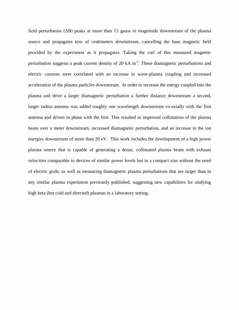
Figure 1.1: Basic Electrostatic Ion Thruster Operation
A cathode at the negative end of the electric potential emits a small number of free
electrons outside the exit grid of the thruster. These electrons are accelerated upstream through
the thruster by the large electric field generated by the high voltage potential. These energetic
electrons collide with neutral gas atoms and ionize them, generating positive ions and additional
electrons. These additional electrons accelerate towards the anode at the rear end of the thruster
and continue the ionization process, while the positive ions are accelerated by the large electric
field towards the cathode. This large drop in electric potential accelerates the positive ions to a
high directed velocity, and as they leave the thruster these ions will generate an electric field
between the ions downstream and the cloud of electrons emitted from the cathode that have not
entered the thruster. This electric field will accelerate electrons from the cathode up to the
velocity of the ions, so that the plasma outflow will be quasi-neutral and the thruster won’t
develop a net charge. The Vex of an electrostatic ion thruster is typically on the order of tens of
km/s, with NASA’s NSTAR-1 engine having an exhaust velocity between 10-30 km/s depending
on the input power [5].
One difficulty with the ion thruster is that the plasma density cannot be increased to
improve the ion outflow and the mass flow rate. If the plasma density were increased, the Debye
length would decrease and more of the interior of the thruster would be shielded from the
accelerating potential drop, decreasing the exhaust velocity. The primary method for increasing

8
the ion outflow rate for an ion thruster is to make the thruster wider and increase the power so as
to provide the same potential drop over a larger volume. These both lead to an increase in
engine mass, so scaling to higher power (more than tens of kilowatts) is difficult.
Section 1.3C: Guiding Plasma Particles with Magnetic Fields and the Hall Effect Thruster
For electrostatic ion thrusters, the plasma density could not be increased because the
electrons in the plasma would adjust themselves to screen out the external electric field as the
Debye length decreased. One method of getting around this problem is to use magnetic fields to
guide and limit the motion of the electrons to prevent them from building up an internal electric
field to cancel out the external field. This is the key process for another standard electric
propulsion system, the Hall effect thruster. The force on a charged particle due to the magnetic
field in the Lorenz force equation (1.6) depends on the direction of motion of the particle relative
to the magnetic field. Motion of the charged particle parallel with the magnetic field does not
exert a force on the particle, while any motion perpendicular to the field direction exerts a force
on the particle perpendicular to both velocity and magnetic field direction. This perpendicular
force on a perpendicular velocity will drive the particle into circular motion around the magnetic
field axis, effectively gyrating around the magnetic field. The motion of the charged particle
gyrating around the field line will be approximately a circle, with the radius determined by the
strength of the magnetic field compared to the momentum of the particle perpendicular to the
field, given by the Larmor radius:
Bq
mvrL
(1.8)
this applies to both the free electrons and the positive ions, and is also referred to as the gyro-
radius. If the Larmor radius of the particle is large compared to the length scale over which the
magnetic field is established, then the particle will not be significantly deflected by the magnetic
field and pass through it in a mostly straight path. If the Larmor radius of the particle is small
compared to the length scale of the magnetic field, then the particle will be gyrating in a tight
orbit around the magnetic field and not move significantly across the field lines. Movement of

9
the particle parallel to the field will still be uninhibited, but movement across the field will be
stopped, and the particle is said to be “well magnetized” and bound to the magnetic field [3].
If the equation for the Larmor radius is re-written to express the perpendicular
momentum in terms of perpendicular temperature for the ions compared to the electrons:
eB
Tmr
ii
Li
2 (1.9)
eB
Tmr
ee
Le
2 (1.10)
it becomes apparent that the ion Larmor radius will be dramatically larger than the electron
radius. The difference in temperature between the two species will typically be negligible
compared to the enormous mass difference between the electrons and the ions. With the
appropriate magnetic field strength the electrons can be well magnetized and bound to the field
lines while the ions are not, which is the requirement for the operation of the Hall effect thruster,
as seen in Figure (1.2).
Figure 1.2: Cross section showing basic operation of a Hall effect thruster

10
The Hall effect thruster has an external cathode that emits electrons and a large voltage
difference between the cathode and the anode to accelerate particles similar to what was present
in the electrostatic ion thruster. The new component to the Hall thruster is a magnetic field that
is perpendicular to the electric field. This magnetic field is intense enough to make the electron
Larmor radius small compared to the size of the thruster while the ion Larmor is large compared
to the thruster. After the electric field accelerates the electrons into the thruster, they begin to
gyrate around the magnetic field and are no longer being accelerated along the electric field.
Instead, they move perpendicular to both fields, in the direction given by:
2B
BEvdrift
(1.11)
as a result of the electron moving both parallel and anti-parallel to the electric field during its
gyration around the magnetic field, resulting in an asymmetric velocity perpendicular to B. With
a sufficiently high electric field, this drift velocity for the electrons can be made sufficiently high
such that a collision between the electron and a neutral atom can produce ionization. This will
generate a positive ion and another free electron, both of which will now feel the effect of the
electric and magnetic fields. The electron will begin to gyrate around the magnetic field and
drift with the other electrons azimuthally around the thruster, which is built with azimuthal
symmetry for this reason. The positive ions will be accelerated by the electric field towards the
cathode and gain a large directed energy, similar to the ion thruster, and their path won’t be
significantly deflected by the magnetic field [3].
Each time the electrons collide with a neutral atom, whether it ionizes the atom or not,
this collision will interfere with its gyration around the magnetic field. This disruption will
temporarily keep it from circling around the field or drifting perpendicular to it, and instead the
electron will be accelerated by the electric field towards the anode. If more neutrals are added to
the system it will result in more collisions and thus more positive ions to be accelerated, but it
will also increase the collision rate with the electrons and therefore the rate at which electrons
will be able to move across the magnetic field and reach the anode of the thruster. These
electrons near the anode will weaken the electric field across the thruster, and lower the directed
velocity of the ions leaving the thruster. Hence a balance is reached: between increased neutral
mass flow into the thruster to dramatically increase the ion outflow rate over the electrostatic ion

11
thruster, and the collisions with neutrals allowing the electrons to move across the field lines and
shield the electrodes from the plasma. The advantage of the Hall effect thruster is the ability to
increase the ion outflow rate by increasing the input power (both of the magnetic field and the
ionizing electron current) without needing to increase the diameter of the thruster. For example,
the Hall effect thruster that powered the SMART-1 space probe launched by the ESA was
smaller in size than the NSTAR ion thruster but achieved similar thrust and exhaust speeds for
similar input power [6].
A problem shared by both electrostatic ion thrusters and Hall effect thrusters is the
erosion of the cathode due to electron loss by emission and through ion impacts. This can act to
limit the lifetime of the thruster, though both thruster types have been operated in space for
thousands of hours and some have been operated continuously for hundreds of hours without the
cathode failing. The larger issue is that of DC electric fields being applied across the plasma
with electrodes, which can then be shielded from the plasma by electrons and their effect limited.
If the formula for the Larmor radius (1.9) is re-written in terms of the angular frequency of the
particles as they gyrate around the field line, called the cyclotron frequency:
m
Bqc (1.12)
it is clear that the lighter electrons will gyrate around the field lines thousands of times faster
than the comparatively heavy ions. If other particles or external fields act on the charged particle
fast enough to interfere with its motion during this gyration, its overall motion will be affected.
This was seen in the case of the Hall effect thruster, where collisions with neutrals interfered
with the gyro-orbit and resulted in limiting the electron’s ability to drift perpendicular to the
field.
Section 1.4A: Oscillating Wave Fields and Electrode-less Helicon Sources
If an externally applied electric or magnetic field oscillates with time at a rate that is slow
compared to the cyclotron frequency of a charged particle, then the particle will go through the
whole gyration with an effectively constant field being applied, and so it will move and drift in a

12
similar fashion to if the field was constant. If the field oscillates at a rate that is fast compared to
the cyclotron frequency, the particle will not have time to move a significant distance in response
to the field before it has changed direction. The particle will be too slow to respond, and the
field will have no net effect on the motion of the particle. The large difference in mass between
the electrons and positive ions puts their cyclotron frequencies far enough to allow a frequency
range such that:
efieldi (1.13)
where ωfield is the angular frequency of the oscillating electric or magnetic field. This oscillating
field will be too fast to significantly affect the ion motion, but too slow to change direction or
strength during the course of an electron’s gyro-motion around a magnetic field. The ability to
inductively drive electric and magnetic fields that can accelerate the electrons without affecting
the ions, and without the use of electrodes, is a key element to the operation of the plasma
sources generally known as “helicons”.
Helicon plasma sources use a helical shaped antenna to inductively drive electric and
magnetic fields to ionize and accelerate plasma without the use of electrodes or grids. The
helicon antennas operate over a range of frequencies, but are in the gap between the ion and
electron cyclotron frequencies as in equation (1.13). The antennas are designed to oscillate at the
resonant frequency of an electromagnetic plasma wave known as a “helicon wave”, which is a
wave of the same form as the “whistler wave” seen naturally in space plasma environments. The
mechanism by which the antenna drives the helicon wave and the details of the wave properties
will be described in Chapter 2.
In general terms, the helicon wave is an electromagnetic perturbation of base magnetic
field B0, with wave components Bw and Ew perpendicular to B0. These wave components twist
around B0 in a helix, and also rotate in time around B0 at the driven frequency in the range given
by (1.13). The wave component is oscillating too fast for the ions to respond, but the electrons
are gyrating around the magnetic field (B0 + Bw) and so when the wave magnetic field vector
rotates in time, the electrons are driven around B0 as well. This rotational velocity for the
electrons is perpendicular to the wave magnetic field Bw, and so the Lorenz force (1.6) acts to
accelerate the electrons along the base magnetic field B0. The rotational velocity is also

13
perpendicular to B0, so there is an additional component of the accelerating the electrons towards
the centerline anti-parallel to Bw. Since the helicon wave is accelerating the electrons and not the
ions, the electrons moving away from the ions build up a strong electric field that acts to
accelerate the ions towards them while decelerating the electrons, the opposite effect to the ions
leaving the electrostatic ion thruster or the Hall effect thruster. This electric field is referred to as
an “ambipolar electric field” and is illustrated below in Figure 1.3.
Figure 1.3: Ambipolar acceleration of the ions by the electrons.
This mechanism allows helicons to drive electrons around a base magnetic field to ionize
neutrals and generate additional electrons and ions, as well as providing a mechanism to
accelerate the plasma downstream out of the thruster without the need for electrodes in the
plasma. Similar to the previous thrusters, a balance will be reached between: strength of the base
magnetic field (B0), input wave energy (Bw), collision rate with the neutrals, plasma density, and
the exhaust velocity of the plasma. This balance will depend greatly on the balance between the
resultant energy of the plasma particles after being ionized and the energy in the magnetic fields.

14
Section 1.4B: Plasma Beta and the Dynamic Plasma Pressure
So far the discussion of the interaction between the plasma and the magnetic field has
involved the interaction of individual charged particles in the plasma with the field, rather than a
collective behavior. A more general way to describe the relationship between the particles of the
plasma and the background field is to consider the relationship between the thermal pressure of
the particles and the magnetic pressure of the background field, called the “plasma beta”:
0
2
2
B
nkTe (1.14)
where n is the plasma density and the contribution of the ions to the thermal pressure is
insignificant. In regions where the magnetic field is high and the magnetic pressure dominates, β
< 1, the electrons (and possibly the ions) will be well magnetized and the plasma will be guided
to flow along the magnetic field lines. When the thermal pressure of the plasma particles
dominates over the magnetic pressure, β > 1, the plasma will expand outward and drag the
magnetic field with it instead of being guided by the field. This is accomplished by currents
flowing in the plasma (driven by the thermal energy) that induce a magnetic field which modifies
the existing field, expanding it out and altering it as the plasma expands. Inside of electric
propulsion devices, magnetic fields used to guide the flow of plasma and help confine the plasma
from interacting with the walls will be strong enough so that β < 1 and the magnetic pressure can
confine the plasma. Once the plasma leaves the thruster however, the plasma needs to move off
of the magnetic field lines attached to the spacecraft so that the plasma does not simply flow
back around and impact the spacecraft. This means the plasma needs to transition to a state
where β > 1 and is no longer dominated by the magnetic pressure [3].
If the thruster relied on just increasing the electron temperature and density to push the
plasma off of the field lines, it would result in a wide thermal expansion of the plasma rather
than a directed flow, with most of the energy not being useful in terms of generating thrust.
Another important relationship for the plasma is the ratio of the directed kinetic energy or
“dynamic plasma pressure” to the magnetic field pressure. This can be written in terms of the
plasma exhaust speed parallel to field in proportion to the Alfven speed, in the form of the
Alfven mach number squared:

15
0
2
2
||
2
||2
B
Vmn
V
VM
ii
a
a (1.15)
which in this case is dominated by the ion terms since their mass is higher. Similarly to the ratio
of plasma beta, if the directed kinetic energy of the plasma dominates over the magnetic pressure
of the plasma, then the plasma will not be guided by the field lines. Instead, the magnetic field
will be dragged along by the plasma as it flows downstream. This will limit the plume
divergence due to following the magnetic field lines, and high parallel velocity along the axis
results in a high exhaust velocity for the plasma plume. Having a high exhaust velocity is
beneficial for a thruster, as shown in the rocket equation (1.5), and so much of the development
work for my experiment focused on increasing the directed ion energies of the plasma plume [7].
Section 1.5A: Overview of Previous Research on the Experiment
The high power helicon (HPH) plasma thruster developed at the University of
Washington was designed to produce a dense plasma that is accelerated downstream at a high
exhaust velocity without the need for electrodes. The HPH accomplished this by coupling
significantly more power into the plasma than other helicons of the time, driving a Bw that was a
significant fraction of B0. This led to non-linear wave interactions with the plasma and resulted
in interesting physics occurring downstream of the plasma thruster. Early investigation by
Ziemba et al. [8] measuring the time of flight of the plasma between points downstream
indicated that the plasma was accelerating downstream of the antenna. It was unclear whether
this acceleration was due to continued interaction with the helicon wave or some other
mechanism, but the measurements showed that the plasma was high beta (β > 1) and super-
Alfvenic (Ma > 1) downstream of the thruster. In addition to the acceleration, the plasma had a
“diamagnetic” effect on the base magnetic field downstream of the thruster, meaning that the
strength of the field was decreased in the presence of the plasma. The diamagnetic perturbation
was small, but not insignificant compared to the weak magnetic field far downstream of the
thruster [9].

16
Further work by Winglee et al. [7] combining multi-fluid plasma modeling with
experimental tests indicated that a magnetic nozzle system, positioned downstream of the plasma
source so that the plasma transitioned to super-Alfvenic in the throat of the nozzle, would result
in a significant increase in exhaust speed combined with a further collimation of the plasma
plume downstream of the nozzle. This suggested that a combination of increased plasma source
power with the right magnetic nozzle geometry could produce a plasma beam that remains
collimated for a significant distance downstream of the thruster [7].
Additional investigation of the ion energies downstream by Prager et al [10] confirmed
that the plasma was accelerating downstream of the plasma source, as well as measuring the
magnetic component of the plasma wave propagating downstream of the antenna. This plasma
wave matched well with a whistler-like wave being launched from the helicon antenna and
propagating along the axis. The diamagnetic signal was again measured, and evidence suggested
it was correlated with the plasma wave and with the increasing ion energies downstream. At the
same time, several other explanations for the ion acceleration were ruled out by the observations
[2].
As a consequence of each of these observations: modifications and improvements were
made to the HPH system to improve thruster parameters such as exhaust speed, plasma density,
and beam width. These modifications included increasing the input wave power, altering the
magnetic field geometry in the plasma source and downstream, adjusting the flow of neutral gas
into the system, and the geometry of the helicon antenna. These changes revealed more
interesting plasma dynamics occurring in the plume downstream of the thruster, and suggested
more elements of the experiment to adjust to improve performance and better understand the
plasma physics governing the behavior of the plasma plume.
Section 1.5B: Overview of this Research on the Experiment:
The high power helicon (HPH) system was intended to satisfy the need for a plasma
source that could be scaled up to high output power levels without significantly increasing the
physical size of the system or requiring grids that can erode and limit the lifetime of the device.
This would be accomplished by designing a system that could use the intense electric and

17
magnetic fields of a non-linear helicon wave to ionize and accelerate a dense plasma to a large
exit velocity without the need for a cathode neutralizing gun or static electric fields. Some
possible applications include: propelling a spacecraft as a thruster, a larger station pushing a
spacecraft with a plasma beam, or a large station de-orbiting space debris by decelerating the
pieces with a plasma beam. Previous work with the HPH [2] [9] had already established that the
helicon source was generating a dense plasma and accelerating it downstream at energy levels
comparable to other plasma thrusters, but had identified problems with the system including
inefficient losses of energy in the source region and weaker coupling of the helicon wave to the
plasma particles downstream of the source.
The first goal of this research was to improve the coupling between the helicon wave and
the plasma particles downstream of the plasma source to increase the output performance of the
device. The methodology for accomplishing the first goal included: characterizing the properties
of the helicon wave downstream of the source with the adjustment of magnetic field and the
orientation of the propagating wave field in a continuation of the work performed by Prager [2],
modifying the source antenna to substantially improve the coupling between the helicon wave
and the plasma particles, and finally measuring the magnetic perturbations of the plasma
particles and their associated currents as a result of interaction with the helicon antenna.
The second goal was to introduce new methods of increasing the power input from the
device into the plasma to further improve the output performance (density, exit velocity) without
significantly increasing the size of the device. The methodology for accomplishing the second
goal included: adjusting the position and intensity of the downstream magnetic field with
magnetic nozzles to improve collimation and acceleration of the plasma beam, and the
implementation of a second antenna downstream to increase the helicon wave power coupling
into the plasma where the loss of energy due to collisions was decreased compared to the source
region.
The most significant new result that arose from accomplishing the first goal was
generation of a much larger diamagnetic perturbation of the background field than had been
previously observed in laboratory plasma experiments with similar plasma properties (density,
temperature). This allows both for laboratory studies of high beta plasmas that were previously
difficult to achieve, and allows a possible mechanism for detaching plasma particles from

18
spacecraft magnetic fields in space propulsion applications. The most significant result from
accomplishing the second goal was the success in using a second antenna to drive additional
helicon wave magnetic field energy downstream and directly accelerate the plasma particles up
to a higher exhaust velocity. This provides a mechanism to further increase the amount of power
the system can input into the plasma without significantly increasing the size of the apparatus,
allowing the HPH system (with further improvements in the future) to fill the niche of a high
power plasma source with exhaust velocities comparable or better to other electric propulsion
devices with similar power levels but in a compact form. The results with the second antenna
also indicate a further collimation of the plasma beam, which would allow the HPH system to be
able to generate a plasma beam in space that can provide thrust over a longer distance to an
object (payload or space debris) than other plasma sources at comparable power levels.
The details of these results, including the large diamagnetic effect achieved by the plasma
source which had not been previously observed in laboratory plasmas, will be presented in the
subsequent chapters.
Section 1.6: Organization of the Dissertation:
The remainder of this dissertation is organized as follows: Chapter 2 will discuss the
experimental apparatus including: the vacuum system, the gas feed system, the magnetic coils
and nozzles, the antenna power supply, and the helicon antenna. The generation of a helicon
wave by the antenna will be discussed, as well as the collisional processes at work between
plasma and neutral particles in the thruster and downstream.
Chapter 3 will introduce the plasma diagnostics used in the experiment to measure the
plasma parameters of the thruster’s outflow. The Langmuir probes used to measure plasma
density and temperature will be described, and deviations from the standard model of the
behavior of a Langmuir probe in our plasma will be discussed. The magnetic coils used to
measure perturbations to the magnetic field will be detailed, as well a more complex electrostatic
probe used to estimate the ion energy distribution in the plasma plume.

19
Chapter 4 will discuss diamagnetic perturbations of the magnetic field measured in the
experiment. These will be compared to observations in other experiments, and the source of the
perturbations will be discussed in terms of the helicon wave versus other possible mechanisms.
Chapter 5 presents estimates of the currents flowing downstream of the source, as
measured by an array of magnetic coils. The shape and dynamics of the current region are
discussed, as well as possible effects on the energies of the ion population downstream of the
current carrying region.
Chapter 6 describes the introduction of magnetic nozzles downstream of HPH and their
effect on ion energy, plasma density, and the perturbation of the magnetic field. Results
indicating improved collimation of the beam and acceleration of the ions will be discussed, along
with some possible options for improvement.
Chapter 7 will present initial results from the introduction of a second helicon antenna
downstream to increase the input wave power into the plasma. Operations at different
frequencies will be compared, and the limitations of the prototype second antenna will be
discussed. Possible improvements for a more effective second antenna will be presented.

20
Chapter 2: Experimental Apparatus
The operation of the high power helicon plasma source (HPH) which is shown below in
Figure 2.1 in a simulated, space-like environment involves several different systems to: establish
a vacuum background similar to space, inject neutral propellant into the system, establish a
magnetic field to confine and direct the plasma, and generate the plasma wave that ionizes and
accelerates the propellant. Each of these sub-systems will be outlined and compared to those
used in other helicon or laboratory plasma experiments. Emphasis will be put on the
characteristics that distinguish the HPH experiment from other plasma sources or thrusters.
Figure 2.1: Picture of HPH Source Firing for 200 μs.
Section 2.1 Helicon Wave:
The helicon wave is a low frequency electromagnetic wave that travels through plasma
along a base magnetic field B0. The wave has electric and magnetic components oscillating
along the guiding magnetic field, with the magnetic field component of the wave (the component
measured experimentally in subsequent sections) given by [11]:

21
tmzkiBB wavewave ||0exp
~, 2.1
where k|| is the parallel wavenumber for the wave propagating along the z axis, m represents the
mode of the wave (m=1 for all the results in this dissertation), and ω is angular frequency of the
wave. The angular frequency of the wave is chosen that it’s well above the ion cyclotron
frequency and well below the electron cyclotron frequency [9]:
ωci << ω << ωce 2.2
so that the ions are relatively motionless over one period of the wave oscillation while the
electrons undergo many gyro-orbits in the same period. The parallel wavenumber k|| is
determined by the plasma parameters and the boundary conditions imposed on the wave.
When there are relatively few boundary conditions, the parallel wavenumber is identical to the
freely propagating whistler wave observed in nature, given by [11]:
ce
pe
ck
|| , 2.3
where ωpe is the electron plasmafrequency. As additional radial boundary conditions are
imposed such as a varying magnetic field, varying plasma density, or a physical boundary, the
behavior of the wave deviates from the unbounded whistler wave. Typical helicon plasma
sources have a uniform magnetic field and an insulating boundary at the walls of the chamber,
leading to a different condition for the parallel wavenumber given by [2]:
kc
kce
pe
2
2
|| , 2.4
where k┴ is the perpendicular wavenumber established by the radial boundary conditions.
Previous work by Prager et al [11] determined that downstream of the HPH source, the parallel
wavenumber closely matched that of the unbounded whistler wave given in eq. 2.3 [11]. With
propagation of the wave parallel to the base magnetic field B0 along the z axis, eq. 2.1 suggests
the wave component of the field Bwave should decrease in θ as z increases, leading to a counter-

22
clockwise (left-handed) rotation around the z axis with position. Equation 2.1 also indicates that
as time increases, θ should also increase leading to a clockwise (right-handed) rotation about the
z axis with time. Both of these characteristics were experimentally observed by measuring Bwave
with the results shown below for four separate times in Figure 2.2:
Figure 2.2: Measured Bwave downstream near 200 μs. The direction of Bwave rotates left-
handed about the z axis moving along the z axis, while each frame shows the wave vectors all
rotating right-handed about the axis as time advances.
The magnetic component of the helicon wave along the z axis shown in Figure 2.2
propagates downstream of the source where there is a base magnetic field and plasma to sustain
it, with more detailed observations described later in Chapter 4. The magnetic and electric field
components of this helicon wave have been described analytically by Chen et al [12] for the case
23
of a uniform magnetic field, uniform plasma density, and an insulated chamber wall boundary.
While this model can match well with experimental results in other helicon experiments with
similar conditions such as in Chen [12], Boswell [13], and others, it does not match well with the
HPH results outside of the source region where the wave is generated. Downstream of the
source the wave behavior more closely matches that of an unbounded whistler wave [11]. The
antenna used to drive this wave is described in the following section.
Section 2.2 High Power Helicon Antenna:
The high power helicon antenna is designed to generate electric and magnetic fields that
couple into the helicon wave which propagates through the plasma. These antenna fields only
line up with the plasma wave fields for part of the time and in a limited location, but with enough
power can overcome the damping mechanisms and generate a helicon wave that can propagate
through the source region and downstream for one or more wavelengths before damping out.
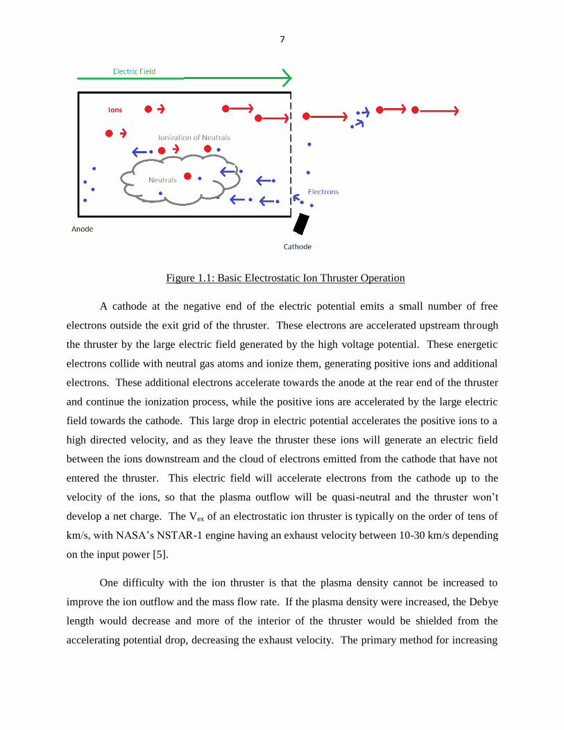
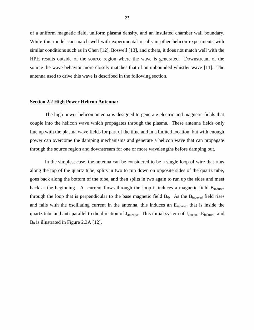
In the simplest case, the antenna can be considered to be a single loop of wire that runs
along the top of the quartz tube, splits in two to run down on opposite sides of the quartz tube,
goes back along the bottom of the tube, and then splits in two again to run up the sides and meet
back at the beginning. As current flows through the loop it induces a magnetic field Binduced
through the loop that is perpendicular to the base magnetic field B0. As the Binduced field rises
and falls with the oscillating current in the antenna, this induces an E induced that is inside the
quartz tube and anti-parallel to the direction of Jantenna. This initial system of Jantenna, Einduced, and
B0 is illustrated in Figure 2.3A [12].
24
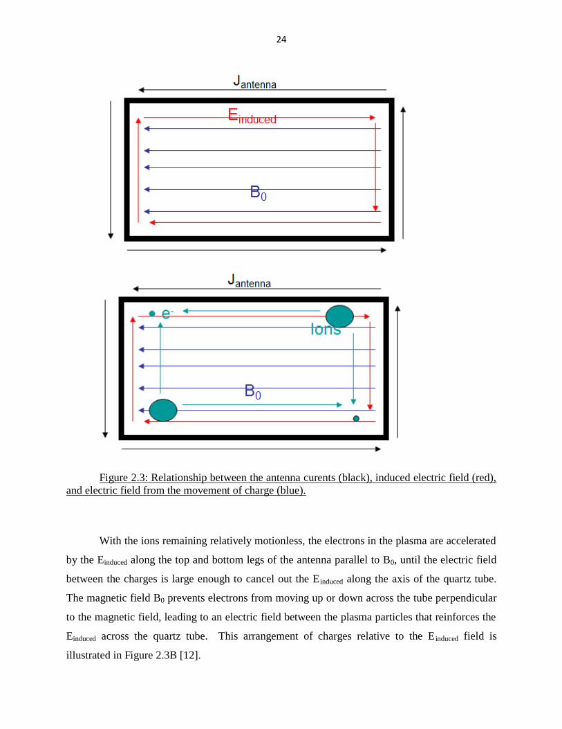
Figure 2.3: Relationship between the antenna curents (black), induced electric field (red),
and electric field from the movement of charge (blue).
With the ions remaining relatively motionless, the electrons in the plasma are accelerated
by the Einduced along the top and bottom legs of the antenna parallel to B0, until the electric field
between the charges is large enough to cancel out the Einduced along the axis of the quartz tube.
The magnetic field B0 prevents electrons from moving up or down across the tube perpendicular
to the magnetic field, leading to an electric field between the plasma particles that reinforces the
Einduced across the quartz tube. This arrangement of charges relative to the E induced field is
illustrated in Figure 2.3B [12].

25
The result is a radial electric field that is perpendicular to the base magnetic field B0,
strongest near the ends of the antenna and switching sign in the middle. Additionally there is the
radial magnetic field (Binduced) across the antenna that doesn’t switch sign in the middle, and both
fields are illustrated in Figure 2.4. A simple loop antenna in this configuration will drive waves
both parallel and anti-parallel to B0.
In order to better match a wave propagating parallel to B0 a left-handed, half-turn twist is
made in the antenna as seen in Figure 2.5. This re-aligns the Einduced to coincide in space with the
Ew of the left-handed helicon wave. This electric field rotates in space with the same handedness
of the helicon wave, but does not rotate in time the same way that the helicon wave does. The
wave fields of the antenna are able to couple into the helicon wave mode for only a limited time,
but are still able to effectively drive the helicon wave.
Figure 2.4: Superposition of induced electric fields across the antenna from the antenna
and the charge add together constructively.
26
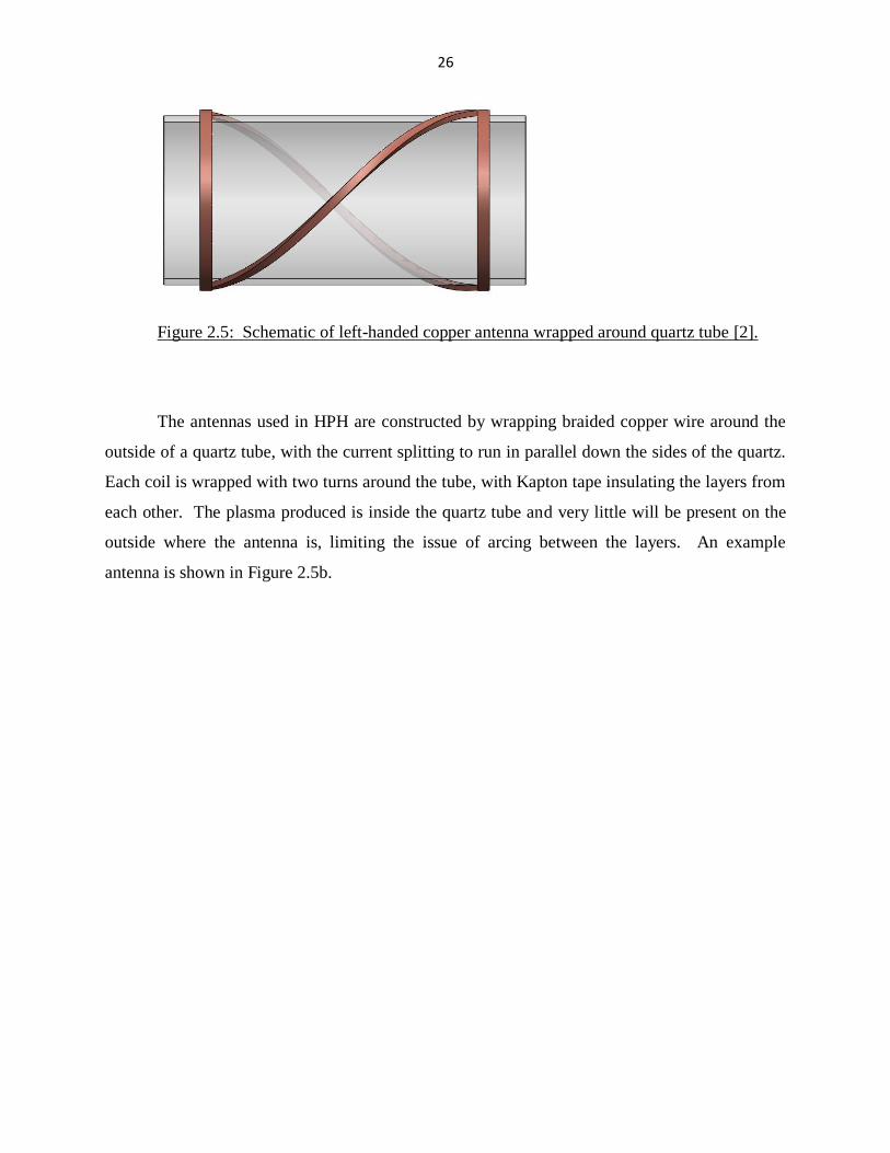
Figure 2.5: Schematic of left-handed copper antenna wrapped around quartz tube [2].
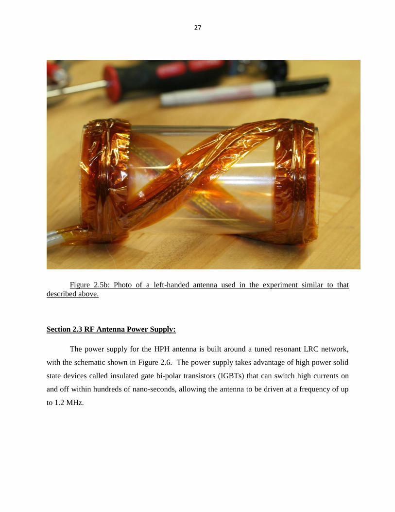
The antennas used in HPH are constructed by wrapping braided copper wire around the
outside of a quartz tube, with the current splitting to run in parallel down the sides of the quartz.
Each coil is wrapped with two turns around the tube, with Kapton tape insulating the layers from
each other. The plasma produced is inside the quartz tube and very little will be present on the
outside where the antenna is, limiting the issue of arcing between the layers. An example
antenna is shown in Figure 2.5b.
27
Figure 2.5b: Photo of a left-handed antenna used in the experiment similar to that
described above.
Section 2.3 RF Antenna Power Supply:
The power supply for the HPH antenna is built around a tuned resonant LRC network,
with the schematic shown in Figure 2.6. The power supply takes advantage of high power solid
state devices called insulated gate bi-polar transistors (IGBTs) that can switch high currents on
and off within hundreds of nano-seconds, allowing the antenna to be driven at a frequency of up
to 1.2 MHz.

28
Figure 2.6: Circuit schematic of tuned LRC network with the antenna operating as the
inductor [2].
On the primary side of the circuit, optical pulses from the control computer trigger the
IGBT driver circuit to close or open the bank of IGBTs. When the IGBTs switch closed: current
flows out of the storage/charging capacitor bank through the transformer and the IGBT bank.
When the IGBTs open again there is a voltage spike across the IGBTs associated with the rapid
decrease in current, which is kept low by a snubbing circuit to keep the voltage spikes from
destroying the circuit. With the IGBTs open, current then flows in the opposite direction through
the diode bank that is in parallel with the IGBT bank, running the opposite direction through the
transformer and re-charging the storage/charging capacitor bank.
On the secondary side of the transformer, the helicon antenna is put in series with a
capacitor bank, forming a resonant LC network with the resistance initially just being the
resistance of the individual components, and later will add in the resistance of the plasma under
the antenna. This capacitor bank is referred to as the tuning capacitor because its capacitance
can be shifted up or down to adjust the resonant frequency of the circuit, given by:
LCf
2
10 2.5

29
where f0 is the resonant frequency in Hz, L is the inductance of the antenna, and C is the
capacitance of the tuning capacitor bank. The storage/charging capacitor is switched on and off
and pulses of current are driven through the primary side of the transformer at the resonant
frequency of the circuit, leading to a large oscillating current at the resonant frequency in the
secondary side of the circuit. With no plasma present the resistance in the circuit is low and the
oscillating current through the antenna builds to large value, ~1500 Amps peak to peak, as seen
in Figure 2.7A. The current oscillates sinusoidally at the antenna frequency until the circuit
stops being driven on the primary side by the computer. Not shown is the voltage across the
antenna, which also oscillates sinusoidally and is typically ~8-10 kilovolts peak to peak.

30
Figure 2.7: Current oscillating in the HPH antenna as a function of time without the
presence of neutral gas (first panel) and with the neutral gas (second panel).
When the antenna is fired with neutral fuel gas present, the antenna will ionize the gas
into plasma and accelerate it out, which draws energy out of the secondary side of the circuit
with the antenna. The plasma acts as an additional resistance in the LRC circuit and puts a load
on the antenna, as seen in Figure 2.7. The oscillating current drops as there is more plasma
Current (No Loading)
-1.00E+03
-8.00E+02
-6.00E+02
-4.00E+02
-2.00E+02
0.00E+00
2.00E+02
4.00E+02
6.00E+02
8.00E+02
1.00E+03
0.00E+00 5.00E-05 1.00E-04 1.50E-04 2.00E-04 2.50E-04 3.00E-04 3.50E-04 4.00E-04 4.50E-04
Time
Am
ps
Current
Current (loading)
-1.00E+03
-8.00E+02
-6.00E+02
-4.00E+02
-2.00E+02
0.00E+00
2.00E+02
4.00E+02
6.00E+02
8.00E+02
1.00E+03
0.00E+00 5.00E-05 1.00E-04 1.50E-04 2.00E-04 2.50E-04 3.00E-04 3.50E-04 4.00E-04 4.50E-04
Time
Am
ps
Current
31
present, and then begins to increase again as plasma is ejected from the source until the antenna
is shut off.
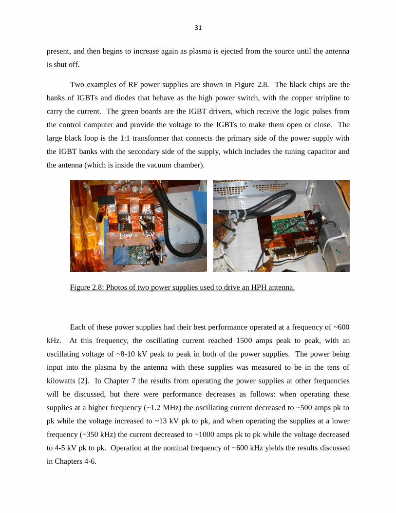
Two examples of RF power supplies are shown in Figure 2.8. The black chips are the
banks of IGBTs and diodes that behave as the high power switch, with the copper stripline to
carry the current. The green boards are the IGBT drivers, which receive the logic pulses from
the control computer and provide the voltage to the IGBTs to make them open or close. The
large black loop is the 1:1 transformer that connects the primary side of the power supply with
the IGBT banks with the secondary side of the supply, which includes the tuning capacitor and
the antenna (which is inside the vacuum chamber).
Figure 2.8: Photos of two power supplies used to drive an HPH antenna.
Each of these power supplies had their best performance operated at a frequency of ~600
kHz. At this frequency, the oscillating current reached 1500 amps peak to peak, with an
oscillating voltage of ~8-10 kV peak to peak in both of the power supplies. The power being
input into the plasma by the antenna with these supplies was measured to be in the tens of
kilowatts [2]. In Chapter 7 the results from operating the power supplies at other frequencies
will be discussed, but there were performance decreases as follows: when operating these
supplies at a higher frequency (~1.2 MHz) the oscillating current decreased to ~500 amps pk to
pk while the voltage increased to ~13 kV pk to pk, and when operating the supplies at a lower
frequency (~350 kHz) the current decreased to ~1000 amps pk to pk while the voltage decreased
to 4-5 kV pk to pk. Operation at the nominal frequency of ~600 kHz yields the results discussed
in Chapters 4-6.
32
Section 2.4 Base Magnetic Field B0:
The magnetic field in the source region serves multiple purposes for the production and
acceleration of the plasma. First, it restricts the flow of electrons perpendicular to the field and
into the walls of the source antenna. When there is sufficient energy in the magnetic field
compared to the thermal energy of the electrons, i.e. that β < 1 as given in eq. 1.14, then the
Larmor radius of the electrons given in eq. 1.9 is small compared to the width of the antenna.
This will limit the motion of the electrons to along the magnetic field lines except for collisions
with neutral particles or ions, which will be discussed later in this chapter.
Second, it allows the source antenna to drive a helicon wave along the magnetic field to
ionize the plasma. The restriction of the electrons from moving perpendicular to the base field
B0 allowed the helicon antenna to generate the radial electric field necessary to couple into the
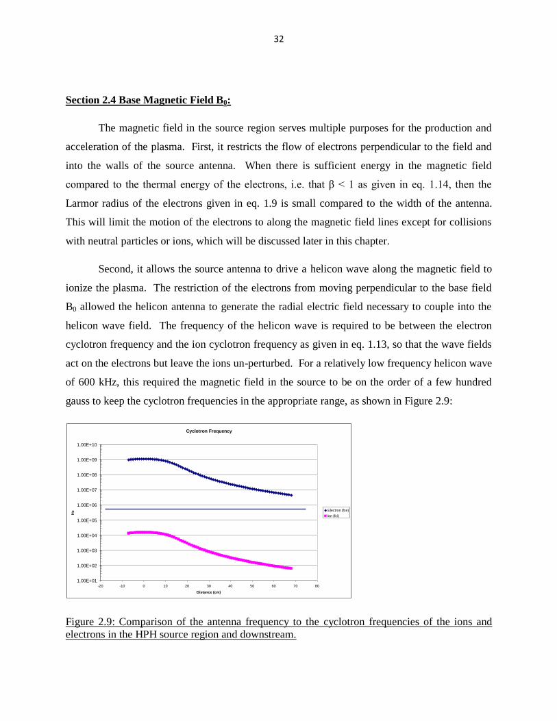
helicon wave field. The frequency of the helicon wave is required to be between the electron
cyclotron frequency and the ion cyclotron frequency as given in eq. 1.13, so that the wave fields
act on the electrons but leave the ions un-perturbed. For a relatively low frequency helicon wave
of 600 kHz, this required the magnetic field in the source to be on the order of a few hundred
gauss to keep the cyclotron frequencies in the appropriate range, as shown in Figure 2.9:
Figure 2.9: Comparison of the antenna frequency to the cyclotron frequencies of the ions and
electrons in the HPH source region and downstream.
Cyclotron Frequency
1.00E+01
1.00E+02
1.00E+03
1.00E+04
1.00E+05
1.00E+06
1.00E+07
1.00E+08
1.00E+09
1.00E+10
-20 -10 0 10 20 30 40 50 60 70 80
Distance (cm)
Hz Electron (fce)
Ion (fci)

33
And lastly, the extended magnetic field allows the helicon wave to propagate along the
magnetic field through the plasma downstream of the antenna. This allows the electron currents
in the plasma to exert a Lorentz force on the plasma particles perpendicular to the current and the
magnetic field at that position. This acts to accelerate the ions and electrons along the axis as the
magnetic field diverges as shown visually in Figure 2.10.
Figure 2.10: The force on the charged ions and electrons for a current flowing around the
axis of the diverging magnetic field results in an acceleration towards the axis and away from the
source region.
The base magnetic field B0 in the source region is generated by six magnetic coils in
series, each 15 cm in diameter and spaced with 3 cm gaps in between, and lined up along the
thruster axis (Figure 2.11). This was done to provide a relatively uniform field near the center of
the magnet, while having the field fall off like a dipole outside the source region. The axial
component of this magnetic field is illustrated in Figure 2.12. The vertical black lines represent
the front and back of the quartz tube. The strength of the magnetic field peaks roughly 1/3rd
of
the way from the back end of the quartz tube and varies by less than 20% over the length of the
antenna.

34
Figure 2.11: Photo of the six magnetic coils used to establish the base magnetic field in
the source region.
Figure 2.12: Profile of the axial component of the magnetic field in the source region and
downstream. The vertical black bars represent the position of the HPH antenna.

35
While most helicon experiments in the past have provided a uniform field for their
experiment both under the antenna and downstream, ours required space-like conditions for the
plasma downstream and that includes a decreasing and diverging magnetic field as the plasma
moves away from the spacecraft.
The magnitude of the base field peaks on axis and is ~400 gauss. This is approximately
what was predicted to be optimal based on the frequency of the antenna, wavelength of the
antenna, and the expected plasma density. The final value we used was determined
experimentally to be the optimal value based on a sweep of the magnetic field. The magnetic
field is established two seconds before the experiment begins and is maintained at a constant
current until after the experimental shot concludes.
Section 2.5 Vacuum Chamber:
In order to simulate space-like conditions my experiments were conducted in a large,
cylindrical vacuum system that is roughly 9’ long and 5’ in diameter, shown in Figure 2.13. The
plasma source is hung from the back end of the chamber within the vacuum environment, to
simulate firing the system in a space environment. Each of the magnetic nozzles, when
implemented, were also under vacuum. A turbo-molecular pump is used to keep the background
neutral pressure of leaked air and outgassed water below 2x10⁻⁶
Torr between shots. The low
neutral pressure limits the collisions between the plasma from the source region and the neutral
particles that aren’t part of the fuel gas in the source. The mean free path for collisions between
the plasma and the neutral background is given by [3]:
nm n
1 2.6
where nn is the background neutral density and σ is the approximate cross section of the neutral
atoms. With the background pressure below 2x10⁻⁶
Torr, the mean free path is >100 m, or well
above the dimensions of the chamber. This makes it unlikely that the plasma will collide with
the air not pumped out of the chamber before it hits the chamber walls, and the neutral
background is sufficiently space-like for this experiment.
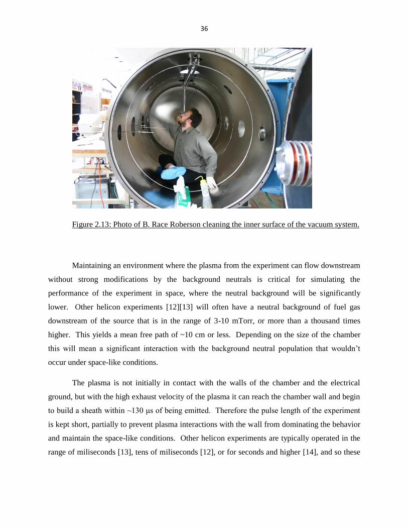
36
Figure 2.13: Photo of B. Race Roberson cleaning the inner surface of the vacuum system.
Maintaining an environment where the plasma from the experiment can flow downstream
without strong modifications by the background neutrals is critical for simulating the
performance of the experiment in space, where the neutral background will be significantly
lower. Other helicon experiments [12][13] will often have a neutral background of fuel gas
downstream of the source that is in the range of 3-10 mTorr, or more than a thousand times
higher. This yields a mean free path of ~10 cm or less. Depending on the size of the chamber
this will mean a significant interaction with the background neutral population that wouldn’t
occur under space-like conditions.
The plasma is not initially in contact with the walls of the chamber and the electrical
ground, but with the high exhaust velocity of the plasma it can reach the chamber wall and begin
to build a sheath within ~130 μs of being emitted. Therefore the pulse length of the experiment
is kept short, partially to prevent plasma interactions with the wall from dominating the behavior
and maintain the space-like conditions. Other helicon experiments are typically operated in the
range of miliseconds [13], tens of miliseconds [12], or for seconds and higher [14], and so these

37
experiments come into equilibrium with the vacuum chamber wall for most of their operating
time.
In the source region when the ionization of the neutrals is taking place, the relationship
between the electron gyrofrequency, electron-neutral collision frequency, and antenna frequency
is given by:
20
cenef 2.7
600 kHz << 22.8 MHz << 1.2 GHz
so that each electron is expected to make many gyro-orbits without colliding with a neutral, but
is expected to collide with many neutrals in one antenna period. The electron gyrofrequency is
determined by eq 1.12 and the electron-neutral collision frequency is determind by [3]:
enne n 2.8
where nn is the neutral density, ve is the electron velocity (which is dominated by the thermal
velocity), and the approximate cross section of the neutral atom. This collision rate increases
with the electron temperature as the velocity of the electrons increase. As the neutrals in the
source are ionized and it switches from low ionization fraction plasma to a high ionization
fraction, the electron-ion collision rate becomes dominant, given by [3]:
e
eei
m
en 2
2.9
where η is the specific resistivity of the plasma, which can be approximated by:
ln4
32
0
2
e
e
kT
me
2.10
with the last term approximated by:
1012lnln3 Den 2.11

38
for laboratory plasmas like those produced by helicons. In the source region once the plasma is
mostly ionized, the electron-ion collision frequency is ~92 MHz. The electron-ion collision is
governed by the electric force between the negative electron and the positive ion when they are
within close proximity. As a consequence, the electron-ion collision rate decreases as the
electron temperature increases because the electron spends less time near the positive ion and is
not as significantly deflected [3].
Once the plasma leaves the source region the neutral density drops dramatically and the
electron-neutral collision rate becomes negligible, but the electron-ion collision rate decreases at
a slower rate given the high plasma density on axis immediately downstream of the antenna. As
the plasma density drops the collision rate decreases, until within about one wavelength of the
source exit the collision frequency has dropped to be on the same order as the antenna frequency.
Section 2.6 Neutral Propellant Injection:
Feeding the neutral propellant gas into the source region at an appropriate rate to sustain
the outflow is difficult. Many of the previous helicon experiments [12][13] fueled the source
region by backfilling the chamber with neutral gas. With neutral gas at a high density filling the
source antenna region and downstream of the antenna, there would be sufficient neutral particles
to flow into the source region from downstream as ions left the source region to sustain the
plasma flow. Work by Chen et. Al. [15] studied how high of a plasma density could be reached
with this method by pointing two helicon antennas at each other in an attempt to build a higher
density plasma between them, and resulted in a lower plasma density because the outflow of
plasma limited the number of neutrals that could flow into the gap between the two helicon
sources. The plasma density was ~8x10¹⁹
m-3
near the exit of each antenna but dropped to half
of that in the region between them.
Other experiments such as VASIMR [14] use a physical choke point between the source
region and the rest of the vacuum system to allow for a high density neutral gas under the helicon
antenna while not having as large of neutral background in the rest of the vacuum chamber.
Converging magnetic field lines in the choke make the plasma density high enough that the flow
of neutrals through the choke is limited. Rather than having the source region neutrals

39
replenished by gas flowing from downstream as above, additional gas flows into the source
region radially from the sides [14].
For HPH to maintain a low neutral background downstream of the source region, while
simultaneously having a high neutral pressure in the source region, we used a fast opening puff
gate to inject neutral gas into the source region with a tube from outside the vacuum chamber.
After 10 ms enough of the neutral gas (typically argon) has flowed into the source to feed the
plasma production, but the pressure downstream of the source has not risen significantly. The
experiment is fired for typically 200-400 μs and the data is collected over a maximum duration
of 1 ms, so the downstream neutral pressure will not change significantly over the course of the
shot. The gas feed is shown in Figure 2.14 by itself in the left panel, and inserted into the back
of the antenna in the right panel of Figure 2.14.
Figure 2.14: The neutral gas feed system shown by itself (left panel) and inserted into the
rear of the source region (right panel).
After the neutral gas puff has expanded to fill the interior of the quartz tube but before it
has had time to expand downstream, an ignitor circuit is triggered to generate a small amount of
seed electrons in the neutral puff for the antenna to immediately act on. The ignitor is a 1500 V
potential drop between two steel grids at the end of the gas feed which draws a current of ~15 A
for 25 μs. The antenna is turned on at the same time and the neutrals begin to be ionized into
plasma. The ionization fraction of the plasma is typically >90% for helicon discharges and the
best way to confirm this for HPH is to look at the line emission spectra from the source region
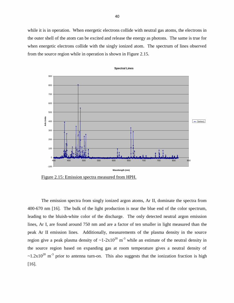
40
while it is in operation. When energetic electrons collide with neutral gas atoms, the electrons in
the outer shell of the atom can be excited and release the energy as photons. The same is true for
when energetic electrons collide with the singly ionized atom. The spectrum of lines observed
from the source region while in operation is shown in Figure 2.15.
Figure 2.15: Emission spectra measured from HPH.
The emission spectra from singly ionized argon atoms, Ar II, dominate the spectra from
400-670 nm [16]. The bulk of the light production is near the blue end of the color spectrum,
leading to the bluish-white color of the discharge. The only detected neutral argon emission
lines, Ar I, are found around 750 nm and are a factor of ten smaller in light measured than the
peak Ar II emission lines. Additionally, measurements of the plasma density in the source
region give a peak plasma density of ~1-2x10²⁰
m-3
while an estimate of the neutral density in
the source region based on expanding gas at room temperature gives a neutral density of
~1.2x10²⁰
m-3
prior to antenna turn-on. This also suggests that the ionization fraction is high
[16].
Spectral Lines
-100
0
100
200
300
400
500
600
700
800
900
400 450 500 550 600 650 700 750 800 850
Wavelength (nm)
Arb
Un
its
Series1

41
Section 2.7 Downstream Magnetic Nozzles:
Two magnetic nozzles were used in the course of my experiments to modify the magnetic
field downstream of the source region. Changing the shape or strength of the magnetic field
outside the source region allowed me to study the effect of the magnetic field of the plasma after
it was created, without significantly altering the production of the plasma in the source region, as
would happen through adjusting the base magnetic field around the source. These two nozzles
are pictured together in Figure 2.16.
Figure 2.16: Photo of the magnetic coils used as magnetic nozzles hanging in the
chamber, centered on the HPH source axis.

42
The first nozzle was designed to be roughly twice the diameter of the base magnets, ~26
cm, and was positioned downstream so that the peak of the nozzle field would overlap the point
where the base magnetic field began to strongly diverge, 20-30 cm downstream. This resulted in
a magnetic field geometry where the magnetic flux diverged after leaving the source, re-
converged through the nozzle, then diverged again slower than before. This had the effect of
lengthening the region where the electrons were magnetized. The axial component of the
magnetic field is plotted in Figure 2.17.
Figure 2.17: Axial component of the magnetic field with a single nozzle added
downstream.
A second nozzle was added, with a diameter twice as large as the first nozzle, ~50 cm,
and the two nozzles were moved in close to the source magnets to limit the amount of the field
re-converging. This new configuration had flux lines that expanded through each nozzle, before
diverging at the exit of the second nozzle. This had the effect of keeping the electrons
magnetized even further downstream, but also limited the amount of flux lines re-converging.
The flux lines were almost everywhere diverging in this configuration. The effect of the nozzles
on the HPH experiment will be discussed in more detail in Chapter 6.
Axial Magnetic Field
0
50
100
150
200
250
300
350
400
450
-10 0 10 20 30 40 50 60 70
Distance (cm)
Gauss No Nozzle
Nozzle

43
44
Chapter 3: Experimental Diagnostics, Theory and Operation
Section 3.1: Summary of the Diagnostics used in the HPH Experiment:
This chapter describes the diagnostic tools used to study the plasma in the High Power
Helicon experiment and some of the basic advantages and limitations of those tools. These focus
on measuring changes to the magnetic field induced by the plasma particles, the plasma density
and electron temperature, and the directed velocity of the ions downstream of the source. These
will be detailed in the following sections.
Section 3.2: Shot to Shot Repeatability of the Experiment
The pulsed nature of the experiment required diagnostics that could measure the
evolution of the plasma as it flowed downstream on a time scale short compared to the
experiment length of a few hundred microseconds. Fortunately the shot to shot repeatability of
the experiment was excellent, and so for electrostatic diagnostics that required a range of
voltages it was straightforward to take a succession of pulses with varying settings. This was
also true when it came to moving probes in position relative to the plasma source to study the
changes with distance from the source as it evolved and flowed downstream. For each data run a
set of control diagnostics was used to determine that the plasma pulses were repeatable,
measuring things like the plasma density in the source region and the input current of the
antenna, while a separate diagnostic was varied in either position or configuration to measure
changes to the plume downstream.
Section 3.3A: Measuring Magnetic Field
The experiment uses a series of magnetic coils to supply a background magnetic field in
the source region and for a short distance downstream. This background field will be perturbed
during the experiment by the actions of the plasma particles and the magnetic field of the plasma

45
waves generated by the antenna. The short pulse length of the experiment made it more practical
to measure changes to the background magnetic field over a few hundred microseconds rather
than measure the total field. Changes to the magnetic field are measured with B-dot coils, which
are coils of fine copper wire that generate a voltage across the output leads proportional to the
change in the magnetic field through the coil based on those described in Hutchinson [4]:
3.1
where N is the number of turns of wire, A is the surface area of the coil, and B is the magnetic
field. Integrating this voltage over time gives the changes in the magnetic field from when the
measurement began. The number of turns and surface area were varied with the coils depending
on the magnitude and length scale of the perturbation being measured. The voltage trace was
also filtered through a combination of hardware and software filters before being integrated
depending on the source of the magnetic perturbation. Depending on its filter, the system could
be used to measure the wave magnetic field that varied at the frequency of the antenna or the
changes to the background magnetic field that varied at a much slower rate.
Section 3.3B: Description of Magnetic Diagnostics
The first magnetic coil of interest was used to measure the change in the axial component
of the background magnetic field along the axis of the thruster. It was ~2 cm in diameter with 25
turns of wire, aligned so the normal of the coil was along the axis of the thruster. The copper
wire and connections were coated in Torr Seal to prevent interaction with the plasma, and the
ring was left open so that plasma could flow through it. The voltage trace was filtered through a
1.5 µs low-pass RC filter to cut down on the antenna noise picked up by the coil, as well as a
second software filter. This diagnostic was used to study the diamagnetic change in the axial
component of the background field due to the plasma and the currents flowing in it, with a time
resolution of ~2 µs. It was mounted on the end of a rod so the coil could be slid along the axis
from 60 cm downstream to within a few centimeters of the source region.
The second magnetic coil used was a set of three perpendicular coils designed to measure
t
BNAV

46
the magnetic field components of the plasma wave driven by the antenna. The probe was made
to be .25 inches in diameter so that all three components of the wave magnetic field could be
measured at approximately the same position. Each coil was made of 50 turns of fine copper
wire, and the set of coils was coated in Torr Seal to prevent interaction with the plasma. This
diagnostic did not use a hardware filter to remove antenna noise, and instead a band-pass filter
was applied in software to filter out the data outside the desired frequency range.
A third set of magnetic coils was made to study the radial profile of the perturbations to
the magnetic field background in finer detail near the axis. This probe contained seven sets of
three perpendicular coils. Each set of coils was ~2 cm in diameter and made with 25 turns of
wire for each set of perpendicular rings. These rings were embedded in nylon rod and covered in
Torr Seal. This line of seven probes in array was hung from a movable track along the top of the
chamber and lowered down into the plasma so that the center of the array was on axis. The track
allowed the array to be moved from 10 cm downstream of the source region out to 60 cm
downstream. The voltage trace from each coil was filtered a 1.5 µs low-pass RC filter, and this
bulk B-dot array was used to study all three components of the perturbation to the background
magnetic field near the axis in detail so that an estimate of the current density could be made.
Each coil of each probe was calibrated using a commercial Bell gauss-meter before being
put under vacuum. This was done by using the gauss-meter to measure the strength of the base
magnetic field accurately, while the probes measured the change in field related to the switching
on and off of the base magnetic field. This allowed the voltage trace over time to be calibrated
with a known magnetic field. Cartesian coordinates are used to relate the direction of the
measured magnetic perturbations and the chamber reference frame: with the z axis along the
thruster axis, the y axis pointed vertically upward, and the x axis perpendicular to the others.

47
Figure 3.1: Orientation of Magnetic Diagnostics relative to source region
Section 3.4A: Measuring Plasma Density and Electron Temperature with Langmuir Probes
Electron density and temperature were measured with a set of Langmuir probes similar to
those described in Hutchinson [4]. These probes operate on the principle of using a bias voltage
on the probe tips to affect the electron and ion currents from the plasma to that surface. One or
more small tungsten electrodes are inserted into the plasma, and are biased with a fixed voltage.
In the case of a single Langmuir probe, the probe tip is biased relative to the chamber wall
(which is attached to earth ground). For a double Langmuir probe, the probe tips can be biased
relative to each other without grounding either. When used in the single probe configuration, a
series of shots are taken in which the bias voltage is varied from strongly negative relative to the
chamber ground to strongly positive relative to the chamber ground. In the double probe

48
configuration the two tips are given a large bias relative to each other, but are left floating
relative to the chamber ground. The current between the probe tips, or between the probe tip and
ground, is measured during the experiment as the plasma interacts with the probe. These
measured currents, taken along with some assumptions about the behavior of the plasma near the
probe tips, give estimates of the electron density and temperature near the probe tips. A brief
summary of the underlying assumptions being made and the basic operation of the Langmuir
probe will be given here, followed by a description of each of the probes used in the experiment.
Section 3.4B: Typical Langmuir Assumptions and Theory of Operation
The initial assumptions for the plasma are that it is quasi-neutral and well thermalized,
with roughly equal numbers of electrons and ions at the same temperature. The positive ions are
all singly ionized of the same species and are assumed to be much more massive than the free
electrons. This plasma is then assumed to be exhausted at speeds much less than the electron
thermal speed into a large vacuum chamber with conductive walls, which are tied to ground.
The free electrons travel to the plasma edge much faster than the ions and so the chamber wall is
hit with significantly more electrons than ions, giving the chamber wall a negative charge
relative to the center of the plasma. This potential difference between the center of the plasma
and the chamber wall is referred to as the plasma potential (Vp), and is usually a few times the
electron temperature in units of eV. Even if the plasma has not yet made contact with the walls,
there will still be a significant potential difference between the center of the plasma and the
plasma edge, as a result of a small deviation from quasi-neutrality with the electrons more likely
to be found at the plasma edge than the center due to their high thermal speed.
This potential difference will act to accelerate the ions in the plasma towards the plasma
edge and the chamber wall, at a rate determined by the electron temperature. Specifically, the
electron interaction with the chamber wall will build up a potential sheath between the wall (at
ground) and the plasma (at Vp), and the ions will be accelerated into the wall through this sheath.
The sheath region is usually not wider than a few Debye lengths, where the Debye length is
defined as:
49
2
1
0
2
0
ne
TeD
3.2
with Te being the electron temperature and n0 being the electron density in the unperturbed
plasma. The Debye length is an approximation of the distance over which electric fields between
the plasma particles effect the motion of the particles, and beyond which there are sufficient
charged particles of opposite charge that the total electric field over the plasma volume is small.
In this case, the electrons have moved to the edge due to their electron temperature and an
electric field is built up, but only over a region on the scale of the Debye length [4].
There is also an extended “pre-sheath” region extending a significant distance into the
plasma from the sheath edge. It is this pre-sheath region’s potential drop that will slowly
accelerate ions towards the plasma edge and the beginning of the sheath. The flux of ions to the
chamber wall will be limited by the rate at which ions drift through the pre-sheath region to the
sheath edge as well as the final speed obtained by the ions falling through the sheath. This final
speed of the ions toward the wall is called the “Bohm speed” and is determined by the electron
temperature, which establishes the size of the potential difference across the sheath.
21
i
eBohm
m
TV 3.3
e
TV e
sheath2
3.4
When a metal probe is inserted into the plasma, a similar sheath develops around the
probe surface area. If the probe is not connected to ground or biased relative to the chamber
wall, then electrons hitting the probe surface will begin to charge the probe until it is negative
relative to the plasma potential. This will continue until the probe is sufficiently negative to
attract an equal (and small) number of ions and additional electrons, so that the total current to
the probe is negligible. This potential is called the “floating potential” because it is the potential
that probes not connected to ground will float to. In order for measurable currents to flow
through the probe and obtain data, the probe will need to be connected either to ground or
another probe tip. The basic case of a single Langmuir probe requires the probe tip to be

50
connected to ground and will be discussed first [4].
When the probe tip is connected to ground, current can flow from the probe to ground
freely. If the probe tip is biased positive relative to ground so that the tip is at the plasma
potential Vp, then there will effectively be no sheath around the probe tip. This will allow all the
electrons impacting the probe to be conducted to ground and with no sheath accelerating ions
into the probe surface the ion current to the probe will be minimal. This will yield a large
negative current to ground, and is generally referred to as being in “electron saturation” since the
probe is collecting all the electrons that interact with it. The next step is to bias the probe tip
negative relative to the plasma potential, by lowering its bias voltage relative to ground. As the
potential on the probe tip gets more negative relative to the plasma potential, more of the
electron population is prevented from impacting the probe surface and the electron current will
decrease. At the same time, the potential difference between the probe tip and the plasma
potential grows and a sheath will form around the probe. The potential difference across the
sheath increases and the ion current to the probe will increase, though it will be limited by the
surface area of the sheath around the probe. Eventually the probe tip will be so negative relative
to the plasma potential that most of the electrons will be repelled from the probe tip and the
current of ions through the sheath to the probe surface will reach a rough maximum determined
by the surface area of the sheath around the probe. This will yield a small positive current to
ground and is generally referred to as being in “ion saturation”, where the probe is collecting all
the ions it can through the probe sheath and very few electrons. This current is given by [4]:
2
1
61.
i
eisheathsat
m
TnAI 3.5
By measuring the current to the probe tip as a function of bias voltage between the ion
saturation point and the electron saturation point, as the electron current to the probe varies from
its minimum to its maximum, an estimate of the electron temperature can be obtained. By
measuring the maximum positive current to the probe at the ion saturation point an estimate can
be made of the ion density, which due to the quasi-neutral assumption of the plasma should
roughly equal the electron density. Since the shot length of this experiment is short compared to
the length of time necessary to gather data over a large range of voltages, a series of shots are

51
taken each with the probe tip biased at a different potential.
For the case of the double Langmuir probe, neither tip is required to be connected to
ground. If both tips are left floating relative to ground, then both tips will be driven by the
electron current to the probes to the floating potential and the current between them will be
minimal. If a bias voltage is applied between the two probes, each probe tip will be biased either
positive or negative of the floating potential. This will allow the negative probe tip to collect
fewer electrons and more ions, while the positive probe will collect more electrons and fewer
ions. This leads to a current from the negative probe tip towards the positive probe tip, in order
to keep the net current to the two probe tips at zero since the probe is floating. As the voltage
difference between the probe tips increase one will be driven towards ion saturation and the other
towards electron saturation. Since the total current to the probe must be zero and the ion
saturation current is small, once the negative probe tip reaches ion saturation a rough maximum
in current is reached and increasing the voltage difference between the tips does not significantly
increase the current measured [4].
As in the case of the single Langmuir probe, measuring the current as a function of bias
voltage can yield an estimate of the electron temperature and the ion saturation current gives an
estimate of the plasma density. In this experiment it was typical to measure the electron
temperature initially to give a rough estimate, and then typically just keep the double Langmuir
probes in ion saturation to estimate plasma density as a function of time and position. While the
electron temperature did vary downstream over the course of the plasma shot, this variability was
small (less than a few eV) compared to the changes in plasma density over the same time.
Section 3.4C: Deviations of the Experiment from the typical Langmuir Assumptions
The initial assumptions that went into the operation of the Langmuir probes do not
entirely apply to this experiment. It is assumed initially that the positive ions and electrons are at
equal temperatures, so that the ion motion is small compared to that of the lighter electrons. In
this experiment the ion temperatures can be significantly colder than the electron temperatures,
but this does not interfere with the “cold ion” assumption being made in the probe description.

52
Another assumption is that there is no impediment of the flow the electrons due to the
magnetic field. In this experiment there are magnetic coils around the source region that
establishes a strong enough magnetic field to magnetize the electrons in the source region and for
a short distance downstream of the antenna, while not effectively magnetizing the ions anywhere
(this will be discussed further in Chapter 4). In this configuration the magnetic field is still not
an impediment to sufficient number of ions and electrons impacting the probe tips. The
Langmuir probes used were typically positioned along the axis of the thruster, so that there was
plenty of plasma available to move along the magnetic field towards the probe without the need
of crossing magnetic field lines. When plasma density was measured off the axis downstream of
the source, it was typically far enough away from the magnet coils that the electron gyro-orbit
was large compared to the size of the Langmuir probe. This means that the effect of the
magnetic field on the estimates of electron temperature and density should be minimal.
The ambipolar electric field generated by the electrons moving away from the ions
accelerates the ions downstream without significantly changing their temperature, so that the
ions instead have high directed energy compared to their thermal energy, flowing downstream
like a cold plasma beam. This has several effects on the behavior of the Langmuir probes. The
first is that it is more difficult to keep ions from impacting the probe surface, so that the floating
potential of the probe is more positive (closer to the plasma potential) than is normal.
Effectively the ion current to the probe is large enough to draw an increased electron current to
the probe to cancel it out.
The second effect is that the Langmuir probes do not easily go into saturation. In the case
of the stationary plasma, a probe tip at the plasma potential or higher can effectively draw in all
electrons nearby and can saturate. The same effect occurs when the tip is at a potential strongly
negative compared to the plasma potential and it effectively draws in all the ions nearby capable
of falling through the sheath. With a steady flow of plasma across the probe there is an increased
supply of ions and electrons to interact with the probe tip. As the potential of the tip increases
further away from the plasma potential, positive or negative, more of the incoming ions or
electrons can enter the sheath and the probe does not saturate as quickly. For the case of ion
saturation, the slope of the current vs. voltage plot decreases when the saturation point nears
rather than approaching zero. For the case of electron saturation, the probe does not reach

53
saturation even for reasonably high voltages of more than a hundred volts. Both of these cases
can be seen in Figure 3.2.
Figure 3.2: Langmuir current as a function of bias potential. At higher positive potentials
the probe does not enter electron saturation, and at negative potentials it does not enter ion
saturation either. Probe current continues to increase with a different slope to the distribution.
The third effect that the flowing plasma has on the Langmuir probes is that in the case of
the double probe that is left floating it is difficult for the probe to establish separate sheathes
around each probe tip that are isolated from each other. In order for the double probe to work it
needs to have two tips close enough to each other that they are still sampling the same volume of
plasma, but far enough apart that a separate sheath forms around each tip to isolate it from the
bulk of the plasma between the tips. This allows for one probe tip to go into ion saturation and
the other tip to draw a sufficient electron current to compensate. With the plasma flowing past
both probe tips, neither tip goes into saturation. As the voltage difference between the probe tips
increase, the width of the sheaths between the probe tips and the plasma extends until they
54
overlap with each other and neither tip now has an effective sheath between it and the plasma. In
this condition current can flow directly from one probe tip to the other tip through the plasma,
leading to a spike in the measured current that is no longer representative of the plasma density.
This will be referred to as “arcing” the Langmuir probe, and unfortunately became more
common as the downstream plasma density and directed velocity increased with improvements
to the experiment.
These difficulties in bringing the Langmuir probes into saturation due to the flowing
plasma required some adjustments to the calibration of our density measurements and introduced
some uncertainties into the estimates of density and temperature. The difficulty in bringing the
double floating Langmuir probes into ion saturation would result in the measurement
underestimating the plasma density, sometimes by as much as a factor of two. In the case of the
single Langmuir probe, the difficulty in getting to electron saturation of the probe meant that the
measurements used to estimate the electron temperature tended to be closer in potential to the
floating potential rather than the plasma potential, which was difficult to estimate. The ease of
getting electrons and ions to impact the probe tended to push the estimates of the temperature to
be hotter than the actual temperature.
Section 3.4D: Description of the Langmuir Probes Used
Several Langmuir probes were used to estimate electron temperature and plasma density
downstream of the source region and in the source region itself. The first Langmuir probe of
interest was designed for use in the source region. It was constructed with two tungsten tips .5
mm in diameter and 3 mm long with a spacing of 3 mm, and was inserted into the center of the
source region along the axis of the thruster. This probe was normally operated as a double
floating Langmuir probe, with voltages typically of 20-60 V across the probe tips. It could also
be operated as a single Langmuir probe when the circuit was biased relative to ground, and the
current from the tip to ground was measured instead, with voltages ranging from -60 V to over
100 V.
The second probe of interest was used to measure plasma density downstream of the
source along the thruster axis. It was constructed with two tungsten tips, 1 mm in diameter and
55
5mm long, and was positioned on along the thruster axis with the tips not shadowing each other
from the flowing plasma. It could be moved as close as 8 cm from the source region and as far
as 60 cm downstream.
Another Langmuir probe used to measure the density of the flowing plasma along the
axis was an asymmetric double Langmuir probe called a planar probe. It was constructed with a
flat disk 7 mm in diameter oriented normal to the flow to collect plasma ions, and a stinger that
was 8 mm long and 1 mm in diameter for collecting electrons. This probe was designed to have
a larger ion collecting surface area to increase the ion current to the probe and increase the
measured current for lower density regions far downstream.
The current for each probe was run through a Stangenes transformer to electrically isolate
the probe tips from the measurement circuitry, and the output signal from each probe was again
filtered with a 1.5 µs low-pass RC filter to cut down on the antenna noise picked up by the wire
leads to the tips.
Section 3.5A: Retarding Field Energy Analyzers:
In addition to the Langmuir probes used to measure plasma density and electron
temperature, additional electrostatic diagnostics were used to look at the energy distribution of
the plasma particles flowing downstream. These diagnostics used retarding electric potentials to
shield a variable amount of lower energy plasma particles from interacting with the probe, and
are referred to as “retarding field energy analyzers (RFA)”. As the retarding potential is raised,
more of the particle population is prevented from reaching the collector until the current reaches
zero. This measures the energy per charge of the particle population reaching the probe. The
RFA diagnostics used in this experiment measured the energy per charge of the ion population
downstream of the source region. Since the plasma population flowing downstream was almost
entirely singly ionized argon, the energy / charge measurement of the RFA could be used to
estimate the velocity of the plasma ions. The exhaust velocity of the plasma as it leaves the
thruster system is critical to the efficiency of the thruster, and is one of the parameters that was
sought to be improved in this experimental work. A brief description of the construction of the
RFA devices and their operation will be given, as well some discussion of the interpretation of

56
the results.
The outer chassis of the RFA is a steel box that is grounded to the chamber, with a small
hole to allow plasma particles to flow into the diagnostic. The interior of the box consists of
several partially transparent (50%) nickel grids, which can be biased to a potential while still
allowing plasma to pass through. Each of the grids is electrically isolated from the others with
ceramic discs. At the far end of the interior is metal disk that collects the ion current of the
particles that made it through the retarding potential. The first grid is positioned right at the
orifice of the RFA box and is tied to ground like the chassis, and is normally referred to as the
“emitter grid”. This prevents the RFA box from drifting in potential relative to the plasma over
the course of the shot. Both ions and electrons will pass through this grid and into the RFA box.
The second grid in the box is the first retarding potential grid, normally called the
“repeller grid”. This grid is designed to repel the plasma electrons from passing further into the
box while allowing the ions through, and is biased -90 V relative to ground. This will turn away
most if not all of the electrons and accelerate the plasma ions through the grid and further into
the RFA. The third grid is biased at a variable voltage and is used to screen out portions of the
plasma ions from passing further into the RFA, normally called the “discriminator grid”.
Initially the grid is tied to ground, and so all the plasma ions that passed through the first two
grids can pass through the third, letting the whole population through. Then a positive bias
voltage relative to ground is added with successive shots, turning back more and more of the ion
population. Eventually the grid is at a high enough potential so that most if not all of the plasma
ions are turned back and cannot pass further into the RFA.
The fourth grid and the collector plate that follows it are both connected to the Stangenes
transformer that measures the ion current to the end of the RFA. The collector plate is biased -
115 V relative to ground, and the fourth grid is biased -18 V relative to the collector plate. This
means that ions impacting the fourth grid or the plate will both add to the signal. This extra grid
is added after the variable retarding potential grid in order to prevent secondary electrons emitted
from the collector plate from escaping. As ions impact the collector plate, some can pull off
more than one electron, and this results in relatively cold electrons being emitted from the
collector plate. If these secondary electrons were allowed to flow from the collector plate to
another part of the RFA, this would result in a current that would appear the same way as ion

57
current to the probe and make the signal higher than reality. The fourth grid, biased negative
compared to the collector plate, turns these electrons back so they impact with the collector again
and so do not generate a current from the plate. But at the same time, any ions that get past the
third grid are the ions the probe is trying to measure, so any ions impacting the fourth grid are
counted as part of the signal. Because of its role in suppressing the secondary electron current,
this fourth grid is normally called the “suppressor grid”. The potential of each grid is plotted in
figure 3.3, with both the maximum and minimum value of the discriminator grid.
Figure 3.3: Graph of electric potential inside RFA chassis
The measured current is run through a Stangenes transformer that electrically isolates the
RFA from the rest of the circuit and steps up the voltage signal. The output voltage is also
filtered with a 1.5 µs low-pass RC filter. The RFA boxes used in this experiment were inserted
radially from the side of the chamber onto the plasma axis downstream of the thruster. They
were fixed in position downstream, but could be rotated so that the input orifice faced the plasma
source or was perpendicular to the plasma source.
RFA Grid Potentials
-150
-100
-50
0
50
100
150
0 0.5 1 1.5 2 2.5 3 3.5 4 4.5
Distance (mm)
Vo
lts
Min Potential
Max Potential

58
Section 3.5B: Interpretation of the Ion Energy RFA Results:
A succession of shots is taken with the RFA, increasing the bias voltage on the
discriminator grid until the ion current to the collector plate is negligible compared to the initial
signal. Plotting current as a function of discriminator voltage indicates what fraction of the ion
population is above a particular energy, directed along the axis of the RFA. Taking the
derivative of this curve with respect to voltage gives the distribution of ion directed energies in
terms of electron volts. Assuming all the ions are of the same species, singly charged argon, the
energy distribution can be plotted as a directed velocity distribution.
A few difficulties in interpreting the RFA results need to be addressed. The first is that
the RFA probe chassis and first grid are tied to the chamber ground when they are placed in the
plasma flow downstream of the source region. Similar to the Langmuir probe, this would
normally mean that a sheath will develop between the RFA and the plasma that would accelerate
ions into the RFA depending on the electron temperature. This would appear in the data as an
increase in the energy of all the ions entering the RFA, an effective shift upwards in directed
energy. As stated earlier in the section discussing Langmuir probe assumptions, this is normally
the case for a stationary plasma, and the sheath does not form in quite the same way for a
flowing plasma such as in this experiment. The clearest way to demonstrate this with the RFA is
to rotate the probe so that the orifice is perpendicular to the axis, and thus perpendicular to the
expected direction of the plasma flow. If there is a sheath formed between the probe and the
surrounding plasma, this sheath should still accelerate ions into the RFA probe when oriented
perpendicular to the flow, since it is clear from radial density profiles that downstream of the
source the plasma flow is significantly wider than the RFA and the probe should be surrounded
by plasma. The results show that the measured ion current drops to zero when the probe is
oriented perpendicular to the thruster axis, which contradicts the idea of a large acceleration due
to a sheath. This also supports the previous results in Prager et al [10] that suggested the ion
beam was cold, and that there is little motion of the ions perpendicular to the flow of the plasma.
Additionally, if the ions were being accelerated by a sheath potential drop of anywhere
between 10 and 50 volts based on the electron temperature, this would be measurable in our
results as it is identifiable in the results of another experiment that uses similar RFA probes. As
a consequence the velocity profile determined by RFA would be significantly higher than in

59
reality, with a bulk velocity increase for the plasma population. However, comparisons between
the bulk velocity determined by the RFA and by time of flight estimates from multiple Langmuir
probes do not show a dramatic difference in the velocity estimate.
A second difficulty in interpreting the RFA data is determining how much of the plasma
ion population makes it through to the end of the RFA and is collected at the suppressor grid or
the collector plate. Each of the grids is only 55% transparent and the channel leading from the
orifice to the collector plate is narrow, only 5 mm in diameter. The two collecting electrodes are
biased at a large negative potential to gather as many ions as possible. It is not known how many
of the ions are lost to the grids or the walls of the RFA, or if there is a segment of the population
at such low directed energy that they cannot reach the collector. Since the RFA probes were all
custom made in house, they have not been calibrated with a known plasma source. Instead, most
of the time RFA data is presented in “Arbitrary Units” rather than in terms of particle flux to
reflect this. The common technique for this experiment is to measure the plasma density at the
same position with a Langmuir probe, and make the assumption that there is no significant
segment of the population that can’t be detected in the RFA, so that the density measurement of
the Langmuir probe can be used to normalize the signal of the RFA to an ion density.
60
Chapter 4: Diamagnetic Perturbations Downstream of the Source
Section 4.1: Plasma Detachment from the Magnetic Field Downstream of the High Power
Helicon
The plasma output of the HPH flows from the source region with a background magnetic
of 300-400 gauss into the expanding dipole region downstream with a significantly weaker
magnetic field, transitioning from a region of low plasma beta to a high beta. Additionally, the
plasma is accelerated out of the source region at >12 km/s, so that it transitions to a super-
alfvenic plasma as the magnetic field strength drops. Determining what effect the dipole
magnetic field of HPH will have on the downstream plasma behavior is critical to understanding
the expected behavior in a space-like environment. The expectation is that downstream the
plasma particle energy, both thermal (represented in the plasma beta of equation 1.14) and
kinetic (represented in the square of the Alfven mach number of equation 1.15), will dominate
over the magnetic field energy density and the plasma will detach from the magnetic field as it
flows away from the thruster. The difficulty is in determining how the electrons will become de-
magnetized and how the plasma particles will warp the magnetic field as they leave the thruster.
One mechanism through which plasma particles become detached from the magnetic
field is through collisions. If the particles are interrupted in the course of their gyro-orbit around
the magnetic field, they will not return to their initial position even if the magnetic field is
uniform over their gyro-orbit. This will allow plasma particles to move perpendicular to the
magnetic field even when the field is strong enough to keep the gyro-orbit small compared to the
scale length of the magnetic field. In the high power helicon experiment the source region is
where the magnetic field is the strongest (300-400 gauss), but it is also the region where the
plasma particles experience the most collisions with neutrals and each other. In the case of the
plasma ions (typically singly ionized argon), collisions with neutrals and other ions keep the ions
from being magnetized. If the ions are assumed to be the same temperature as the electrons and
well thermalized (the ion-electron collision frequency is ~90 MHz), then for Ti = 10 eV the ion-
neutral collision frequency and ion-ion collision frequency are both ~500 kHz, which is larger

61
than the ion gyrofrequency of ~15 kHz [17]. This means that the ions could not complete their
gyro-orbits without multiple collisions, so they can’t be magnetized to the source field.
Additionally, the gyro-orbit of the ions at 10 eV is larger than the antenna diameter, so that the
ions would hit the walls of the source antenna before completing the orbit. If the ions are
assumed to be much colder than the electrons, such as 1 eV, than the gyro-orbit of the ions is
small enough to fit within the confines of the antenna. However, as the ion temperature drops
the coulomb collision frequency between the ions in the source region dramatically increases to
~18 MHz, making it less likely that the ions could complete a gyro-orbit before colliding with
each other. If the ions have an anisotropic temperature, such as with a higher temperature
parallel to the magnetic field than perpendicular to allow a higher ion temperature while keeping
the ion gyro-radius small, then we still expect the scattering of the ions from the ion-neutral
collisions to keep the ions from completing their gyro-orbits and being well magnetized. In
summary, it is expected in the source region that collisions prevent the ions from being
magnetized by the base magnetic field.
In the case of the electrons in the source region, the lighter free electrons are expected to
be magnetized. With the intense magnetic field the electron gyro-radius is ~0.2 mm and the
gyrofrequency is ~1.1 GHz, which is roughly a factor of ten larger than the frequency of
collisions for electrons in the source region. Initially as the neutral population in the source
region is high while the plasma is being ionized, the electron-neutral collision frequency is ~0.11
GHz, while later in time when the plasma is mostly ionized the electron-electron collision
frequency of ~0.16 Ghz and the electron-ion collision rate of ~0.09 GHz dominate. These
collision rates are high enough to expect some transport of electrons perpendicular to the field
and into the walls of the antenna, but the higher gyrofrequency suggests that the electrons go
through many gyro-orbits between collisions and the bulk of the electrons will be magnetized by
the base magnetic field in the source region [17].
In the region immediately downstream of the source, when the magnetic field is
decreasing like a dipole and the collision rate is dropping, different mechanisms come into play
for detaching plasma particles from the magnetic field. In the case of the ions, the collision
frequencies are still larger than the gyro-frequency of the ions, so they will still not be
magnetized to the field lines of the source magnets. Also, the ion gyro-radius has become large

62
compared to the scale-size of the magnetic dipoles maintaining field, so the ions are not expected
to see a uniform magnetic field over their gyro-orbit. This is in contrast to the case of the plasma
electrons, where the collision rate between the electrons and the other particles has decreased
faster than the magnetic field has dropped off. This is due to the significantly decreased neutral
population in the vacuum chamber downstream of the source, as well as the decrease in the
plasma density as the plasma is expanding. The neutral population was measured with a
capacitive monometer over the course of a typical shot. After the field has decreased to ~100
gauss the electron gyro-frequency is ~280 MHz, while the highest collision frequency is the
electron-electron collision rate of ~1.6 MHz. Collisions are no longer a practical mechanism for
detaching electrons from the magnetic field, and two other mechanisms begin to play the
dominant role.
As the ions move away from the source region they are not well magnetized to the base
magnetic field, while the electron still are. As the two populations begin to separate, ambipolar
electric fields are generated to accelerate the electrons towards the ions and vice versa. The
electrons have difficulty moving across the magnetic field to reach the ions which are more
massive and respond slower to the ambipolar electric fields than the electrons. The two
mechanisms to bridge this gap and maintain quasi-neutrality are: the electrons finding an
alternate path to the ions, and the modification of the magnetic field to allow electrons to move
more freely. In the first case the electrons are able to take advantage of the conducting chamber
wall of the experimental apparatus to find an alternate path to the ions. The plasma begins to
reach the chamber wall and build up a sheath between the conducting wall and the plasma within
100 µs of the experiment being turned on. The large thermal speed of the electrons, ~1,800
km/s, allows the free electrons to be able to move along the magnetic field from the source
region to the chamber wall, move along the conducting surface of the steel wall, and then back
along the magnetic field in a short period of time compared to the ion movement across the
magnetic field, which is in the range of 5-20 km/s. Another path the electrons can take is back
into the source region: by following the field back into the source region, collisions can allow the
electron to move perpendicular to the field given sufficient time, and then travel out of the source
region closer to the dipole axis of the magnetic field and winding up further downstream with the
ions. It is expected that once there is sufficient contact between the plasma and the chamber
wall, more electrons will take the first path because it doesn’t rely on a longer collision time to

63
move across the magnetic field. In this case the electrons are not yet fully detached from the
magnetic field, but are in effect able to move across the magnetic field by using the conducting
chamber wall.
Figure 4.1: Top down view of dipole magnetic field lines emerging from the source
region and connecting to either the conducting chamber walls or the ambient magnetic field of
the Earth, directed down. Ion motion across the magnetic field lines forces the electrons to take
a longer path through the conducting chamber wall when they cannot modify the magnetic field.
The second mechanism by which the electrons can become detached from the magnetic
field of the source is plasma particles modifying the magnetic field. As the ions are
demagnetized and the electrons aren’t, the gyromotion of the electrons around the field relative
to the ions (which aren’t gyrating) generates an electric current that is diamagnetic to the base
magnetic field. This will weaken the magnetic field, increasing the electron gyro-orbit and
making it easier for the electrons to move across the field. If there is sufficient thermal energy
density in the electrons compared to the magnetic energy density of the base magnetic field, that
is if plasma beta is > 1, then this will create a diamagnetic cavity where the magnetic field is low
-1
-0.8
-0.6
-0.4
-0.2
0
0.2
0.4
0.6
0.8
1
-0.4 -0.3 -0.2 -0.1 0 0.1 0.2 0.3 0.4 0.5 0.6 0.7 0.8 0.9 1 1.1 1.2 1.3 1.4
Impacts Side of Chamber
Connects to
Ambient Earth
Magnetic Field

64
enough for electrons and ions to both pass through without deflection by the field. Across this
cavity, and particularly at the edge, there will be a large variation in the local magnetic field and
the electron gyro-radius. The electron gyro-radius will be large inside the cavity and small at the
edge, leading to a diamagnetic current at the edge of the cavity to sustain it. Similar to how the
local magnetic field is reduced inside the diamagnetic cavity, the field is increased at the edge of
the cavity where the field of the diamagnetic current and the field from the source magnets
reinforce each other. The electrons inside the cavity will be demagnetized because their gyro-
radius will be large compared to the length-scale of the source magnetic coils and the
diamagnetic cavity diameter. The electrons at the flanks of the cavity (where the field is
reinforced) will remain magnetized until the field gets so weak that their gyro-radius is also large
compared to the length scale of the background magnetic field. This detachment of the electrons
from the base magnetic field of the source by modification of the magnetic field is expected to be
the dominant mechanism if the experiment were fired in space without the conducting chamber
boundary.
The last point to consider in terms of the interaction between the plasma particles and the
magnetic field is when the plasma has moved far enough away from the source that the base
magnetic field is no longer dominant over the Earth’s magnetic field. Instead of flowing along a
diverging magnetic dipole field, the plasma will now be moving perpendicular to a relatively
uniform weak magnetic field with a scale length that is large compared to the chamber. Previous
experimental observations of the HPH plasma in this region showed the plasma moving across
the magnetic field seemingly unhindered, at roughly the same velocities as closer to the source
region. This is similar to other laboratory experiments such as those by Wessel et al [18] where
a plasmoid was launched perpendicular to a uniform magnetic field and passed through it
without modifying the magnetic field or slowing down. In that case as the plasmoid moved
across the magnetic field, the differential motion of the ions and electrons due to the Lorenz
force developed a polarization electric field across the plasmoid that was perpendicular to both
the magnetic field and the direction of motion. The ExB drift of this electric field combined with
the perpendicular magnetic field accelerates the ions and electrons in the plasma in the original
direction of flow, so that the plasma flows across the magnetic field at approximately the same
speed as if the magnetic field wasn’t there at all [18].

65
For the case of the high power helicon firing perpendicular to the ambient Earth magnetic
field (~0.5 gauss) the ion gyro-radius is significantly larger than the chamber while the electron
gyro-radius is ~20 cm. The electron gyro-orbit is small enough for the electrons to complete
their orbits without hitting the chamber wall or colliding with other particles, so we’d expect the
electrons to be significantly deflected by the Lorentz force as they moved across the magnetic
field. If the electrons are moving perpendicular to the flow independent of the ions, a
polarization electric field could be expected to develop across the plume to allow the plasma to
flow across the magnetic field with little change in velocity. The electric field would be weak
enough that we wouldn’t expect any significant deflection of the ions, but the ExB drift of this
field on the electrons should act to move them across the magnetic field in the flow direction to
keep up with the ions. Whether this effect would dominate over the previously mentioned
mechanism where the electrons flow along the chamber wall to keep up with the ions is unclear,
but in both cases there would be little to no modification of the background magnetic field as the
plasma flows past and little to no change in velocity of the ions.
The experiment by Wessel et al [18] also showed that there was significant deflection of
their plasma beam when it was fired into a perpendicular magnetic field that also contained an
ambient plasma density that was comparable to the density of the moving plasmoid. In that
example, the polarization electric field was reduced to almost nothing, resulting in a large
divergence of the plasmoid beam [18]. The same would likely be true when firing the HPH
across a magnetic field in space with an ambient plasma density that was comparable to that of
the plume. We would expect a significant change in the behavior of the plume as it interacted
collisionlessly with the ambient plasma, either exerting a pressure to push it aside and modifying
the magnetic field at that location, or diverging rapidly as it moved across the field with little to
no polarization electric field.
To summarize the detachment of the plasma from the background field of the HPH
source, the ions are not particularly well magnetized anywhere. The electrons are magnetized in
the source, with some losses across the magnetic field due to collisions. Downstream of the
source the electron collision rate has dropped so that collisions aren’t the dominant mechanism
for moving electrons across the magnetic field. The bulk of the plasma is near the thruster axis
and is mostly traveling along the magnetic field, but near the flanks where the ions are moving
66
across the magnetic field the electrons most likely keep up by moving along the chamber wall
instead of modifying the magnetic field. Near the axis there is a significant diamagnetic
modification to the magnetic field and it’s expected that the electrons are demagnetized in this
diamagnetic cavity and follow with the ions. Details of the diamagnetic perturbation are
presented later in this chapter. Farther downstream of the source where the magnetic field is
weaker the ion gyro-radius becomes larger than the chamber while the electron gyro-radius
reaches ~20 cm, so that electrons still have difficulty moving across the magnetic field when
they are far enough from the walls to make complete orbits. As the plasma flows across the
ambient magnetic field of the Earth, most likely a polarization electric field forms and allows the
plasma particles to flow across the magnetic field without slowing down.
Section 4.2: High Beta Effects and Diamagnetic Perturbations in Laboratory Plasmas
One of the mechanisms mentioned in the previous section for detaching plasma particles
from the base magnetic field was a large diamagnetic decrease of the magnetic field near the
axis. A diamagnetic current develops when the gradient in the plasma pressure is perpendicular
to the magnetic field, with the plasma pressure trying to push the plasma across the field and the
Lorentz force keeping the plasma particles from moving outwards. As the diamagnetic current
develops it acts to weaken the strength of the magnetic field to allow greater expansion of the
plasma at the expense of thermal energy from the plasma particles. For this reason the local
magnetic field strength will be expected to decrease in the case of large plasma beta, where the
plasma pressure gradients are higher and there is more thermal energy available compared to the
background magnetic field [3].
In the general case of a high beta plasma that is stationary relative to a background
magnetic field, the plasma thermal pressure of the electrons acts to push the magnetic field out of
the plasma leading to a diamagnetic decrease of the magnetic field inside the plasma. For
plasma beta > 1 this could lead to a complete expulsion of the magnetic field from the plasma,
with a large diamagnetic current flowing through the plasma to sustain this change in the
magnetic field, with the field decreasing on a time scale related to the conductivity of the plasma
[19]. When the plasma is instead moving from a region of low magnetic field into a region of

67
higher magnetic field, the plasma pressure should push aside the magnetic field and have it pile
up until the magnetic pressure can balance the plasma pressure, both thermal and dynamic. The
opposite case of plasma flowing from a strong magnetic field into a weaker one should result in
the plasma warping the magnetic field to push the higher background field into the region of
weaker field by driving internal currents to oppose the change in the magnetic field. These
effects are seen most commonly in high conductivity space plasmas like the solar wind, which is
a high beta plasma that extends the magnetic field of the Sun into the solar system as the
interplanetary magnetic field, and exerts a pressure on the magnetospheres of planets like Earth
[20].
Laboratory plasmas with electron temperatures in the range of 5-10 eV can still be built
up to high plasma beta by increasing the density of the plasma or lowering the background
magnetic field. The low electron temperature and higher plasma density results in more frequent
coulomb collisions, which increases the resistivity of the plasma and the rate at which magnetic
field will diffuse through the plasma. There are also significant loss mechanisms for the
laboratory plasma such as recombination and interaction with the chamber wall that aren’t
present in the space plasma environment. The combination of these loss mechanisms has the
effect that in the laboratory environment high beta plasmas produced with dense electron
populations of 5-10 eV do not produce the same magnetic perturbations that are common in
space plasmas where these loss mechanisms don’t play a role.
The effects of high beta plasmas on their surrounding magnetic fields in the laboratory
environment have been demonstrated with limited success. An experiment by Stenzel et al [21].
conducted in a uniform background axial field (B0 = 5 G, ne ≤ 8x10¹¹
cm-3
, kTe ≤ 5 eV) was able
to cancel the base field for a plasma thermal beta ratio of 5 but not for β thermal = 1 as would be
expected. Even though βthermal exceeded unity for more than 150 μs in the afterglow of the
discharge, the magnetic field returned to ~5 G much faster than expected based on diffusion of
the field into the plasma. The return to 5 gauss of the magnetic field was correlated in time with
the loss of the high energy tail of electrons (kTe ~ 50 eV) that were responsible for light
production in the discharge and not with the bulk thermal electron population providing the
plasma pressure used to estimate βthermal [21] as shown in the following paragraphs. It is a
similar situation to what is seen downstream of the HPH, where the electrons are mostly

68
magnetized to the field with a limited collision rate while the ions experience too many collisions
along their orbit to be well magnetized to the field.
One key difference is that the plasma downstream of the HPH source is flowing outward,
while the experiment by Stenzel et al [21] features mostly stationary plasma that is sustained
near the axis of the chamber against plasma loss rate towards the walls, with the magnetic field
limiting the flow of plasma perpendicular. This gives a pressure gradient towards the axis where
the plasma density is highest, and this pressure gradient drives a diamagnetic current that acts to
weaken the magnetic field on axis where the plasma density is highest, effectively forcing the
magnetic flux off the axis and piling it up at the flanks of the plasma column. However, since
the ions are unmagnetized they can flow across the field away from the axis driven by the
pressure gradient while the electrons cannot move across the field. This builds up an electric
field and the ExB drift of the electrons due to this field is opposed to the diamagnetic drift of the
electrons. Stenzel et al [21] concluded that these opposing electron motions caused the
diamagnetic signal to significantly decrease, forcing the plasma beta to be greater than 1 to expel
the magnetic field from the axis. An experiment conducted by Banerjee et al. [22] under similar
conditions reported that even with βthermal ~ 10 their base magnetic field was not entirely
cancelled on axis.
A more recent experiment was performed by Corr et al. [19] with a helicon source firing
into a dipole field along the axis. Their results indicated a 2% decrease along the axis of the 34
G base field for βthermal = 2, or a total field change of < 1 gauss. Their magnetic field strength
was high enough to magnetize the ions in the plasma plume, unlike the case of Stenzel et al. [21],
but they also concluded that the lack of a strong diamagnetic signal was the result of the field
rapidly diffusing into the plasma [19].
Unlike other laboratory experiments, the high beta plasma flowing from HPH is shown in
the following to significantly distort the magnetic field downstream, exhibiting a diamagnetic
perturbation that is 2-5 times higher than what was previously observed. In this chapter I
describe these diamagnetic perturbations and their evolution with time in the downstream plasma
plume. This includes a diamagnetic decrease along the axis that indicates a complete expulsion
of the background magnetic field, which will have significant impact on how the plasma near the
axis detaches from the magnetic field and flows away.

69
Section 4.3: Diamagnetic Perturbations in Previous HPH Results
In the early work on the high power helicon (HPH) experiment, Ziemba [9] also
measured a perturbation of the base magnetic field downstream of the source. It developed as
the plasma flowed downstream and lasted for a few hundred microseconds. It was a few gauss in
strength on the axis and was diamagnetic, similar to what was measured by Stenzel [21] and
Corr. [19]. The measurement was made with a radial cut across the source region, showing a
diamagnetic perturbation that peaked on the axis and fell off away from the source near the
chamber walls.
Early estimates of the plasma velocity downstream of the high power helicon (HPH) by
Ziemba et al [8] using the time of flight between Langmuir probes revealed that the plasma was
accelerating downstream of the source, with the bulk of the plasma traveling at 4 km/s within the
first 15 cm, but traveling at 7 km/s by the time it was 70 cm downstream. It was uncertain at the
time whether this acceleration was due to the formation of a double layer similar to that seen by
Charles et al [23], or if it could be the result of the helicon wave continuing to couple energy into
the plasma downstream of the source region. Measurements of the directed ion energies (>20
eV) by Prager [10] with a retarding field energy analyzer (RFEA) similar to that of Conway et al
[24] indicated that the Alfvén mach number was greater than unity within 10-20 cm of the source
region along the thruster axis.
In order to characterize the helicon wave downstream of the plasma source and determine
if it could be responsible for the downstream plasma acceleration, Prager [2] measured the
magnetic component of the helicon wave downstream of the source with an integrated B-dot coil
near the frequency of the antenna (~560 kHz). Estimates of the wavelength (~30 cm) closely
matched what was expected given the length of the half-wave antenna (15 cm). The wave
magnitude was strongest near the source and decreased along the axis, propagating through the
plasma as far as 60 cm downstream [2]. At the same time, an axial measurement of the
diamagnetic perturbation was made, showing a similar perturbation as was previously measured
(at most a few gauss), that also extended down the axis as far as 60 cm downstream. This
perturbation was correlated in position and time with the wave magnetic field, with the

70
perturbation disappearing within tens of microseconds of the antenna being turned off and the
wave was no longer being driven [2].
To further study whether the measured helicon wave was responsible for the diamagnetic
perturbation and the downstream acceleration of the plasma, I modified the antenna and power
supply of HPH to have a left-handed pitch similar to the type ‘R’ antenna discussed by Light et
Al [25]. To test the coupling between the new antenna and power supply, data was taken with
the wave propagation and plasma flow anti-parallel to the magnetic field as it was for the work
by Prager [2], as well as with the flow parallel to the field. The case with anti-parallel
propagation resulted in a diamagnetic perturbation of at most a few gauss similar to the previous
results, but with the field directed parallel to the field there was a dramatic increase in the
magnitude of the diamagnetic perturbation measured downstream. The two cases are plotted
together compared to the base magnetic field in Figure 4.2.
Figure 4.2: Axial diamagnetic perturbation relative to the base magnetic field. The red trace is
for propagation anti-parallel to the magnetic field, while the blue trace is for parallel propagation.
The green trace is the magnitude of the base magnetic field

71
The two cases displayed in Figure 4.2 are for the same magnetic field magnitude, helicon
antenna, and input power from the antenna. The only difference is the direction of the magnetic
field compared to the direction of plasma and wave propagation. The anti-parallel propagation
case has a peak in the perturbation of ~2 gauss as previously observed, peaking near the antenna
and decreasing in magnitude down to a fraction of a gauss 60 cm from the plasma source. In
contrast, the diamagnetic perturbation in the parallel propagation case is ~4 gauss near the source
antenna and then increases to a peak of ~16 gauss roughly 20-30 cm downstream. At this point
the diamagnetic perturbation is about the same magnitude as the base magnetic field but in the
opposite direction, suggesting the total magnetic field on the axis is ~0 gauss. Further
downstream the diamagnetic perturbation decreases from this peak at the same rate the base
magnetic field decreases, maintaining the condition of the magnetic field being near 0 along the
axis. To study this dramatic increase in the diamagnetic signal, magnetic probes were used to
study the perturbation near the axis along with axial measurements of the wave magnetic field
similar to those conducted by Prager [2]. These results are presented in the following sections.
Section 4.4: Diamagnetic Perturbations along the Axis
The base magnetic field of HPH falls off like a dipole field and drops in magnitude from
hundreds of gauss near the exit of the source down to the terrestrial field strength within 1.5 m of
the source. This was done to simulate space-like conditions where it is not feasible to maintain a
uniform field far downstream of the spacecraft.
The planar probe indicated a flowing plasma population similar to that seen in Prager [2],
with the peak density decreasing as the probe is moved further from the source. The antenna was
shut off at 200 μs and the decrease in the downstream density is delayed by the time it takes the
plasma to flow downstream at the bulk plasma speed. This plasma density is shown as function
of time in Figure 4.3 for axial locations at 15 cm, 30 cm, and 45 cm (with time relative to the
antenna activation). These density data are compared with the measurement of the perturbation
to the bulk magnetic field along the axis at the same location. Prior to the arrival of plasma at
the locations 15 cm and 30 cm downstream there is no change in the bulk magnetic field. Within

72
~10 μs of the plasma density increase the B-dot detects a diamagnetic change in the bulk axial
magnetic field at that same position.
Figure 4.3: The axial component of the measured magnetic perturbation (Gauss) is shown in the
dashed line along with the electron density profile shown in the solid line at the same location.
The direction of the ΔB was diamagnetic, decreasing the total magnetic field.
The diamagnetic perturbation increases over a period of ~30 μs at each of the
downstream locations in Figure 4.3 and builds to a peak value of 8-12 G. At each position the
∆B begins to fall with time after 110 μs and decreases to ~2 G which is more typical of earlier
measurements. This suggests the perturbation is decreasing with time either because the
population of particles carrying the diamagnetic current are propagating away or being damped
out (independently of the bulk population measured by the planar probe), or because the effect is
being damped out by plasma increasingly interacting with the chamber wall.
At 200 μs the antenna is shut off and at each point downstream in Figure 4.3 the magnetic
perturbation decays away in less than 10 μs, even though the density measurements indicate that
source plasma is still flowing downstream from the helicon for more than 10 μs after shutoff.
This is similar to the results of Stenzel et al [21] in which their diamagnetic perturbation
disappeared within 100 μs of their source being shut down, even though the measured plasma
pressure still indicated a βthermal >1. This indicates that part of the diamagnetic perturbation late
in time is being driven by the source antenna, and is strongly damped out as soon as the source is
shutoff.
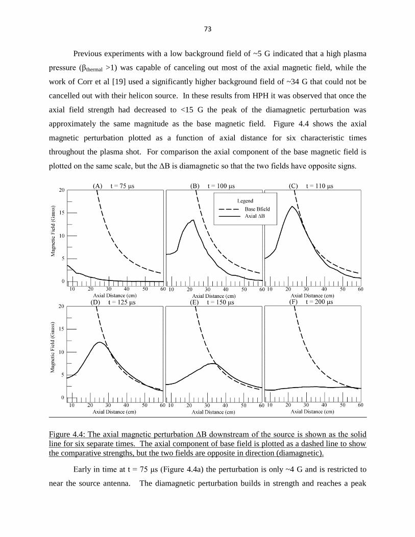
73
Previous experiments with a low background field of ~5 G indicated that a high plasma
pressure (βthermal >1) was capable of canceling out most of the axial magnetic field, while the
work of Corr et al [19] used a significantly higher background field of ~34 G that could not be
cancelled out with their helicon source. In these results from HPH it was observed that once the
axial field strength had decreased to <15 G the peak of the diamagnetic perturbation was
approximately the same magnitude as the base magnetic field. Figure 4.4 shows the axial
magnetic perturbation plotted as a function of axial distance for six characteristic times
throughout the plasma shot. For comparison the axial component of the base magnetic field is
plotted on the same scale, but the ΔB is diamagnetic so that the two fields have opposite signs.
Figure 4.4: The axial magnetic perturbation ΔB downstream of the source is shown as the solid
line for six separate times. The axial component of base field is plotted as a dashed line to show
the comparative strengths, but the two fields are opposite in direction (diamagnetic).
Early in time at t = 75 μs (Figure 4.4a) the perturbation is only ~4 G and is restricted to
near the source antenna. The diamagnetic perturbation builds in strength and reaches a peak

74
value of >15 G on axis at 110 μs (Figure 4.4c), between 20 and 30 cm downstream of the plasma
source. The perturbation falls off in intensity farther downstream in Figure 4.4c, but beginning
at ~25 cm downstream the perturbation is comparable to the base magnetic field. The magnitude
of the perturbation roughly follows the fall in strength of the axial base magnetic field
downstream of the peak. In time the peak of the perturbation shifts further downstream,
decreasing in magnitude with the base magnetic field as shown in Figure 4.4d and Figure 4.4e
and canceling the axial field downstream of the peak. By the time of antenna turnoff at 200 μs,
the magnetic perturbation has become a more uniform ~2 G field along the axis, which is still
large enough to cancel the base magnetic field at 50 cm downstream. This large diamagnetic
perturbation of the field (>15 G) is significantly higher than what was measured with previous
versions of HPH or reported in other helicon sources. This indicates that from 110 μs and later
in time there is an extended region along the axis downstream where the magnetic field has been
fully expelled from the axis and the axial component of the total magnetic field (the dominant
local field) is ~0.
Section 4.5: Comparison of Diamagnetic Perturbation with Helicon Wave Magnetic Field
A smaller 3-axis magnetic field probe was used to observe waves propagating
downstream of the source similar to those of Prager et al [11] and was described in Chapter 3.
The temporal and spatial evolution of the wave magnetic field is directly tied to the evolution of
the total axial magnetic field, as shown for six times in Figure 4.5. The external base magnetic
field provided by the dipole magnets and the diamagnetic perturbation to the axial field are
combined to form a total axial field represented by a dashed curve.

75
Figure 4.5: Comparison of the wave magnetic field magnitude (solid line) to the total axial
magnetic field magnitude (dashed line) downstream of the source at six times. Downstream of
the source the wave magnetic field driven by the antenna is comparable to the axial magnetic
field.
As the oscillating wave magnetic field propagates downstream with the plasma it is
initially bound by the edge of the plasma, but as the total field begins to drop when the external
magnetic field is expelled from the axis the wave magnetic field is clearly being bound on the
right-hand side by the drop in axial magnetic field as seen in Figure 4.5c. The wave magnetic
field decreases in magnitude following the axial magnetic field, dropping from ~2 G 25 cm
downstream in Figure 4.5b to ~0 G at the same position in Figure 4.5c.
Later in time in Figure 4.5d and Figure 4.5e the point at which the axial magnetic field drops to
zero has moved farther downstream, and the wave magnetic field has propagated farther
downstream as well, still following the decrease in the axial magnetic field. This is good
evidence that the external magnetic field is being 100% expelled from this region near the axis

76
because the helicon wave requires a base magnetic field to propagate, the lack of the helicon
wave suggests that the local field strength is ~0. Beginning at 150 μs it is possible that the wave
field is beginning to penetrate into the region at a lower magnitude, perhaps because the
diamagnetic effect has begun to damp away and it no longer is completely expelling the field.
The ratio of the wave magnetic field to the total axial field in Figure 4.5 is significant
because most helicon sources are thought to produce a linear plasma wave, with the wave
magnetic field being a small perturbation of the total field. In the case of the High Power
Helicon (HPH), the plasma wave being produced by the source is a non-linear perturbation of the
wave field, being perhaps >10 G in the source region (compared to 400 G peak base field), and 4
G downstream of the source when the total axial field has dropped to ~4 G. This region where
the wave magnetic field is the same magnitude as the total field could be part of the explanation
why the peak in the diamagnetic perturbation occurs so far downstream of the source, since the
diamagnetic effect is at least partially driven by the antenna late in time.
Section 4.6: Correlating Antenna shutoff and Diamagnetic Perturbations in time
In order to further correlate the dramatic drop in the diamagnetic perturbation along the
axis with the shutoff of the helicon antenna and the loss of the helicon wave being generated, the
shot length of the experiment was varied over several hundred microseconds. Figure 4.6
compares the axial diamagnetic signal compared to the base magnetic field for the case of three
different shot lengths for the 20 μs immediately following turnoff.
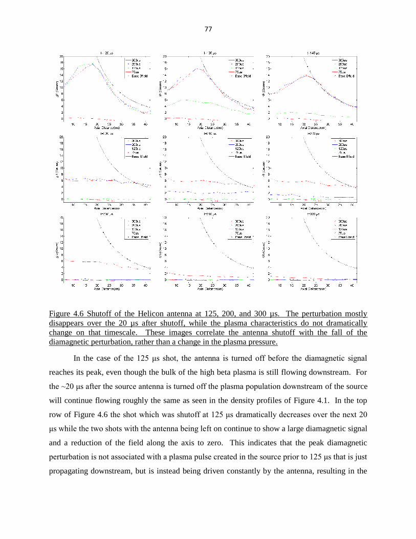
77
Figure 4.6 Shutoff of the Helicon antenna at 125, 200, and 300 µs. The perturbation mostly
disappears over the 20 µs after shutoff, while the plasma characteristics do not dramatically
change on that timescale. These images correlate the antenna shutoff with the fall of the
diamagnetic perturbation, rather than a change in the plasma pressure.
In the case of the 125 μs shot, the antenna is turned off before the diamagnetic signal
reaches its peak, even though the bulk of the high beta plasma is still flowing downstream. For
the ~20 μs after the source antenna is turned off the plasma population downstream of the source
will continue flowing roughly the same as seen in the density profiles of Figure 4.1. In the top
row of Figure 4.6 the shot which was shutoff at 125 μs dramatically decreases over the next 20
μs while the two shots with the antenna being left on continue to show a large diamagnetic signal
and a reduction of the field along the axis to zero. This indicates that the peak diamagnetic
perturbation is not associated with a plasma pulse created in the source prior to 125 μs that is just
propagating downstream, but is instead being driven constantly by the antenna, resulting in the

78
early shutoff case in the top row of Figure 4.6 never reaching the same peak perturbation
downstream as in the two shots where the antenna was left on longer.
For the second row of Figure 4.6, the diamagnetic perturbation has settled into a uniform
perturbation of 5-6 gauss for a long distance downstream. When the antenna is shutoff at 200 μs,
the diamagnetic perturbation again damps out rapidly while the plasma population downstream is
again relatively unchanged. The shot which remains on for 300 μs maintains the same uniform
perturbation for another 100 μs until it is shutoff in the third row of Figure 4.6. This indicates a
relatively stable value for at least a few hundred microseconds for the diamagnetic perturbation
to achieve. Again, the diamagnetic perturbation drops immediately when the antenna is shutoff.
The rapid decrease in the diamagnetic signal measured on axis when the antenna is
shutoff indicates that the diamagnetic perturbation isn’t simply being carried by the plasma
downstream, but is being driven by the antenna and is being strongly damped by another
mechanism, so that the magnetic field on axis returns to normal within ~20 μs.
Section 4.7: Estimate of the Diffusion Rate for Magnetic Field onto the Axis
In both the Stenzel et al [21] and Corr et al [19] experiment, rapid diffusion of the
magnetic field into the plasma is suspected to be the reason why the diamagnetic signal is
smaller than expected. Following the example of Corr et al [19], they estimated that for
magnetic field diffusing into a collisional stationary plasma, the characteristic time would be
given by:
2
0 L (4.1)
where L is the characteristic length scale of the magnetic field (in this case the radius of the
magnetic dipole) and η is the resistivity of the plasma assuming that the dominant term is the
coulomb collision of electrons and ions, which is true downstream of HPH. For a laboratory
plasma with an electron temperature of ~10 eV like in the case of the collisional region
immediately downstream of HPH, η ~ 1.65x10⁻⁵
ohm-m. Plugging in the dipole magnet radius
79
of ~7 cm, this yields a value of τ ~ 375 μs. This time scale is longer than the value from Corr et
al [19] of ~50 μs, where colder electron temperatures of 5 eV and below were used. In this case
we’d expect the time needed to diffuse the magnetic field from the edge onto the centerline to be
on the order of hundreds of μs for a 5-10 eV plasma. This is long compared to the rapid falloff
in diamagnetic signal measured on axis of the HPH, which is usually on the order of tens of μs.
This suggests that the plasma is either far more collisional than estimated so far, or there is a
separate mechanism responsible for the rapid drop in diamagnetic field when the antenna is
switched off.
Section 4.8: 2-D Spatial Variations of Diamagnetic Perturbations Near the Axis
To study how the perturbation of the base field changes near the axis in finer detail, an
array of seven, 3-axis bdots was used. This probe array was described in Chapter 3 and
produced a 2D data set that is ~50 cm long and ~12 cm wide in a vertical plane along the axis of
the thruster. The z component of the B-dot array was used to measure the axial component of
the diamagnetic field perturbation and ΔBz is shown as a function of position for four separate
times in Figure 4.7. The scales on the plots are distorted due to the probe being able to move a
much farther distance axially downstream than the radial width of the probe array.
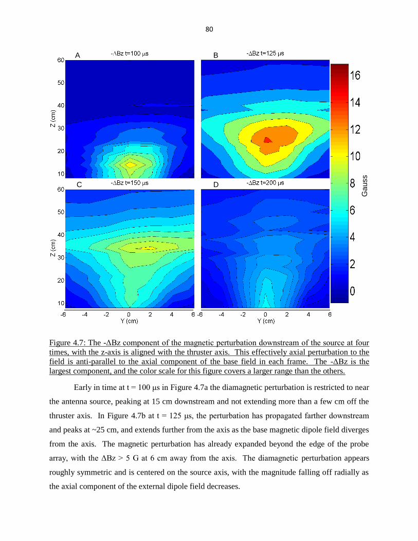
80
Figure 4.7: The -ΔBz component of the magnetic perturbation downstream of the source at four
times, with the z-axis is aligned with the thruster axis. This effectively axial perturbation to the
field is anti-parallel to the axial component of the base field in each frame. The -ΔBz is the
largest component, and the color scale for this figure covers a larger range than the others.
Early in time at t = 100 μs in Figure 4.7a the diamagnetic perturbation is restricted to near
the antenna source, peaking at 15 cm downstream and not extending more than a few cm off the
thruster axis. In Figure 4.7b at t = 125 μs, the perturbation has propagated farther downstream
and peaks at ~25 cm, and extends further from the axis as the base magnetic dipole field diverges
from the axis. The magnetic perturbation has already expanded beyond the edge of the probe
array, with the ΔBz > 5 G at 6 cm away from the axis. The diamagnetic perturbation appears
roughly symmetric and is centered on the source axis, with the magnitude falling off radially as
the axial component of the external dipole field decreases.
A
C D
B
Ga
uss

81
This evolution in time is similar to the results of the axial probe: a diamagnetic
perturbation is built up downstream and propagates away from the source, with the peak of the
ΔBz roughly equal to the base magnetic field strength, leading to a cancellation of the field as the
peak moves past it and expelling the external field. Figure 4.7 indicates that the magnetic
perturbation is not just limited to near the source axis but is part of a large diamagnetic effect
over an extended region downstream of the source. If the decrease in axial magnetic field near
the axis was due to flux being pushed outward by the diamagnetic effect as was thought in
Ziemba [9], it would appear in the data set as an increase of the base magnetic field on the radial
edge of the ΔBz or further downstream of the source. There is no indication of an enhanced
axial field in the bulk B-dot array results near the axis in Figure 4.7, though it is expected it be
there in order for the divergence of the magnetic field to be zero. It is possible that the increase
in flux would only be measurable tens of centimeters off the axis as was seen previously, which
would put it too far off axis to measure with this probe array centered on the axis.
The y-axis of the bdot array is oriented vertical to the ground and perpendicular to the
thruster axis, so that the y-axis gives effectively the radial component of the magnetic
perturbation, taking into account the change in sign across the axis. The ΔBy component of the
magnetic perturbation is shown as a function of position for four separate times in Figure 4.8.
Early in time in Figure 4.8a, ΔBy is limited to within 15 cm of the source antenna and peaks a
few cm off the axis. The sign of the ΔBy is opposed to the y component of the base magnetic
field, pointing radially inwards towards the axis while the diverging dipole base field is pointed
away from the axis, indicating that this is a diamagnetic perturbation as well. This suggests that
early in time and near the source, the region in which the external field is entirely expelled is
extending radially off axis for at least a small distance.
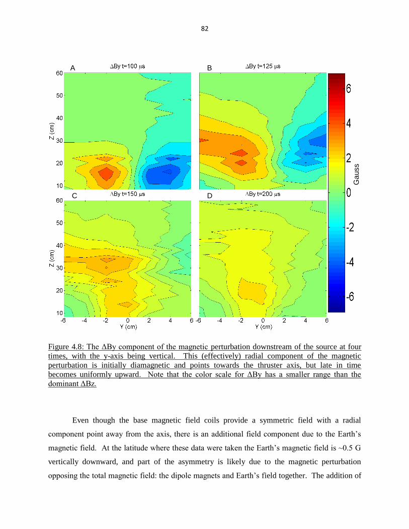
82
Figure 4.8: The ΔBy component of the magnetic perturbation downstream of the source at four
times, with the y-axis being vertical. This (effectively) radial component of the magnetic
perturbation is initially diamagnetic and points towards the thruster axis, but late in time
becomes uniformly upward. Note that the color scale for ΔBy has a smaller range than the
dominant ΔBz.
Even though the base magnetic field coils provide a symmetric field with a radial
component point away from the axis, there is an additional field component due to the Earth’s
magnetic field. At the latitude where these data were taken the Earth’s magnetic field is ~0.5 G
vertically downward, and part of the asymmetry is likely due to the magnetic perturbation
opposing the total magnetic field: the dipole magnets and Earth’s field together. The addition of
A
C D
B
Ga
uss
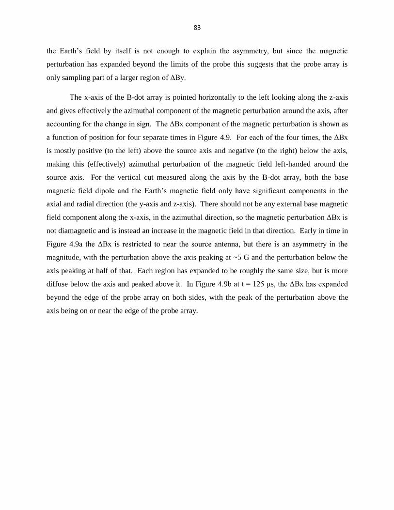
83
the Earth’s field by itself is not enough to explain the asymmetry, but since the magnetic
perturbation has expanded beyond the limits of the probe this suggests that the probe array is
only sampling part of a larger region of ΔBy.
The x-axis of the B-dot array is pointed horizontally to the left looking along the z-axis
and gives effectively the azimuthal component of the magnetic perturbation around the axis, after
accounting for the change in sign. The ΔBx component of the magnetic perturbation is shown as
a function of position for four separate times in Figure 4.9. For each of the four times, the ΔBx
is mostly positive (to the left) above the source axis and negative (to the right) below the axis,
making this (effectively) azimuthal perturbation of the magnetic field left-handed around the
source axis. For the vertical cut measured along the axis by the B-dot array, both the base
magnetic field dipole and the Earth’s magnetic field only have significant components in the
axial and radial direction (the y-axis and z-axis). There should not be any external base magnetic
field component along the x-axis, in the azimuthal direction, so the magnetic perturbation ΔBx is
not diamagnetic and is instead an increase in the magnetic field in that direction. Early in time in
Figure 4.9a the ΔBx is restricted to near the source antenna, but there is an asymmetry in the
magnitude, with the perturbation above the axis peaking at ~5 G and the perturbation below the
axis peaking at half of that. Each region has expanded to be roughly the same size, but is more
diffuse below the axis and peaked above it. In Figure 4.9b at t = 125 μs, the ΔBx has expanded
beyond the edge of the probe array on both sides, with the peak of the perturbation above the
axis being on or near the edge of the probe array.

84
Figure 4.9: The ΔBx component of the magnetic perturbation downstream of the source at four
times, with the x-axis being horizontal. This (effectively) azimuthal component of the magnetic
perturbation is a left-handed perturbation around the thruster axis. Note that the color scale for
ΔBx has a smaller range than the dominant ΔBz.
The three axes of the B-dot array taken together suggest that the magnetic perturbation is
a macroscopic effect that begins near the source region and expands downstream and radially
away from the source building up to a peak value. Then the perturbation propagates downstream
off the edge of the probe array as well as expanding radially away from the axis beyond where
the probe can measure. Near the time when the antenna has turned off there is an extended
A
C D
B
Ga
uss

85
region downstream with a magnetic perturbation ≥1 G and near the source the perturbation is
still >5 G until the antenna is turned off, at which point the magnetic perturbation disappears
within tens of microseconds. The ΔBz diamagnetic perturbation is the dominant term, building
to a peak >15 G more than one antenna length away from the source. The ΔBy term was in
some cases diamagnetic but was also asymmetric later in time above the axis. The ΔBx term
was not diamagnetic because there was no base magnetic field in the x direction along the axis of
the probe array.
Section 4.9: Summary of Diamagnetic Perturbation Data:
Early tests of the previous version of the HPH system using anti-parallel wave
propagation exhibited diamagnetic perturbations at most a few gauss, similar to what has been
published associated with other helicon plasma thrusters. This was originally a radial profile
which peaked on axis and was not large enough to cancel out the base magnetic field, even with
the plasma beta >1 and the plume being both supersonic and super-alfvenic [9]. Subsequent tests
using a modified version of HPH measured an axial diamagnetic perturbation of the magnetic
field of at most a few gauss along the thruster axis downstream as far as 60 cm. The helicon
wave was also measured along the axis downstream to determine how far the wave was
propagating and how quickly the wave was damping out away from the source antenna [2].
Initial tests of the version of HPH that I used for my research were done with the magnetic field
reversed so that the wave and plasma were propagating anti-parallel to the field. This
configuration produced a diamagnetic perturbation of a few gauss, similar to what was seen with
the previous HPH system. It was not until the magnetic field was aligned downstream that the
large diamagnetic perturbations were observed.
The peak in the diamagnetic perturbation downstream increased by almost a factor of 10
after the magnetic field was aligned downstream, with the wave and the plasma both propagating
parallel to the field. The peak in the diamagnetic perturbation is measured 20-30 cm downstream
of the source where the magnitude of the base magnetic field has decreased enough for the
perturbation to roughly cancel out the field from the magnets, for a net field of ~0 on axis.

86
Beyond this point the diamagnetic perturbation decreases in magnitude roughly as the base
magnetic field falls, so that the perturbation cancels out the field but does not seem to reverse it.
The perturbation decreases with time down to a value of ~2 gauss which is similar to
previous results and other experiments, but the decrease is not associated with a change in the
bulk plasma density. Plasma density downstream of the source is relatively uniform as the
perturbation decreases in magnitude over the shot length. After the antenna is shut off, the
perturbation decays away within tens of microseconds even far downstream of the antenna, while
the plasma population decreases as a slower rate because plasma is still flowing downstream
from the source.
When comparing the magnitude of the wave magnetic field along the axis with the
diamagnetic perturbation, two interesting properties are observed. The first is that the wave
magnetic field strength drops to zero in the region along the axis where the diamagnetic
perturbation has cancelled out the base field. This is further confirmation that the field along the
axis is ~0, since the helicon wave needs a magnetic field to propagate along. The second
interesting property is that the wave magnetic field is roughly equal to the total magnetic field
strength in the region just upstream of the large diamagnetic perturbation. This is further
evidence of the non-linear nature of the HPH plasma wave. Initially the magnitude of the wave
magnetic field is >10 gauss but decreases over time as the wave reaches farther downstream.
This most likely indicates that the wave energy is piled up near the source region early in time
before the plasma has had time to move farther downstream and the diamagnetic decrease in the
field also acts to keep it restricted close to the source. Over time the plasma expands farther and
the diamagnetic perturbation is weaker but over a larger region, at the same time the wave
magnetic field is measured further along the axis.
When the antenna is shut off the diamagnetic perturbation decreases in strength rapidly,
even far downstream of the source. This is independent of the plasma population which
decreases on a slower time-scale once the antenna is shut off, and at the time of antenna shut off
is still high beta enough to suggest a large diamagnetic effect. When estimating the time needed
to have the background magnetic field diffuse back through the conducting plasma along the
axis, the time predicted based on the conductivity is larger than what is observed. This suggests

87
that there is a strong damping mechanism at work that is overpowered by the antenna while it’s
on, but quickly damps out the diamagnetic perturbation once it is shut off.
The diamagnetic perturbation is three dimensional, with the strongest component being
the axial diamagnetic perturbation. There is an additional radial perturbation that is opposed to
the diverging base magnetic field, pointing inwards towards the axis when strongest. There is
also an azimuthal magnetic perturbation that is not diamagnetic because the expanding dipole
field from the source doesn’t have an azimuthal component. This component is left-handed
around the axis and is a few gauss in strength, suggesting perhaps that either some magnetic field
is being twisted into a left-handed shape, possibly associated with an axial current with electrons
flowing out along the axis and returning along the flanks. The diamagnetic perturbation extends
not only far downstream, but also a significant distance away from the thruster axis. The 2D
data of the magnetic perturbations near the axis, combined with some assumptions about
symmetry, can be used to estimate the strength of the currents in the plasma that are generating
the perturbations. The discussion of these currents and the broader question of the source of the
diamagnetic perturbations will be discussed in Chapter 5.

88
Chapter 5: Estimated Diamagnetic Currents based on Diamagnetic Perturbations and Discussion of Ion Energy Enhancement
Section 5.1: Estimating Current Density from Magnetic Perturbations:
The volume of plasma downstream of the source has only been partially measured with
the diagnostics available, but with some assumptions of symmetry an estimate of the currents
produced can be developed. The first assumption that must be made is that the plasma plume
and the magnetic perturbation are azimuthally symmetric. This allows the 2D cut from the bulk
B-dot array presented in chapter 4 to provide sufficient information to determine the downstream
current density. Previous measurements of the plasma density with Langmuir probes support
this assumption, indicating a mostly symmetric plasma plume downstream.
From the differential form of the Maxwell-Ampère equation:
J
DB
t0 (5.1)
The magnetic perturbation we measure is present for longer than 100 μs, and the dominant axial
component of the ΔB suggests that the curl of the magnetic field perturbation is predominantly in
the azimuthal direction around the plasma axis. This makes it unlikely that there are azimuthal
displacement fields building up for the bulk of the plasma shot time. So if we assume that
displacement fields are small, then:
JB 0 (5.2)
The spatial resolution in the magnetic field perturbation measurements is limited to 2 cm over an
area that is 12 cm wide by 52 cm long, and since the curl of the magnetic perturbation depends
on the partial derivatives, the estimates of the current density are further limited. In the Cartesian

89
coordinates used in the lab measurements (where ‘z’ is parallel with the thruster axis and ‘y’ is
vertically upward) [3]:
zyxB
y
B
x
B
x
B
z
B
z
B
y
B xyzxyz (5.3)
The partial derivatives with respect to y and z can be read from the B-dot array results, only the
derivatives with respect to x are absent. The xBz in the second term of eq. 5.3 can be
assumed to be small because of the observed symmetry of the ΔBz. Only the xBy in the third
term of eq. 5.3 can still complicate the assumption of azimuthal symmetry. Therefore if we are
assuming azimuthal symmetry and that the vertical yz plane that the probe measured is typical of
any cut across the plasma, we expect it to be accurate with the possible exception of a correction
to the current density in the z direction along the axis.
Section 5.2: Estimated Azimuthal Diamagnetic Current:
The x component of the curl represents an azimuthal current around the source axis and is
shown as a function of position for four separate times in Figure 5.1. The (effectively) azimuthal
current is left-handed about the thruster axis, in the same direction as the azimuthal magnetic
perturbation. The current peaks 2-3 cm off the source axis and is ~20 kAm-2
in density. The
high current density is the result of the sharp radial decrease of the ΔBz away from the source
axis, suggesting a current source that is restricted to a few square centimeters near the axis.

90
Figure 5.1: Estimated Jx current density downstream of the source at four times. The
(effectively) azimuthal current is oriented left-handed about the axis, such that the field that
would be induced by this current has its normal anti-parallel to the base magnetic field, resulting
in the axial diamagnetic field.
Early in time in Figure 5.1a, the region with azimuthal current has extended roughly one
antenna length (15 cm) downstream. The current density peak reaches ~20 kA m-2
at 2-3 cm
from the axis and has decreased to 5 kA m-2
at the edge of the probe array, suggesting that the
effect does not extend much farther beyond the edge of the array. At t = 125 μs in Figure 5.1b,
the Jx region has expanded to 30 cm downstream and radially off the edges of the probe array,
but the peak of the Jx remains within 4 cm of the axis and >15 kA m-2
. In Figure 5.1c the peak of
the current density has decreased to ~10 kA m-2
and is peaked near the helicon source rather than
1-2 antenna lengths downstream. The current drive region extends downstream but has grown
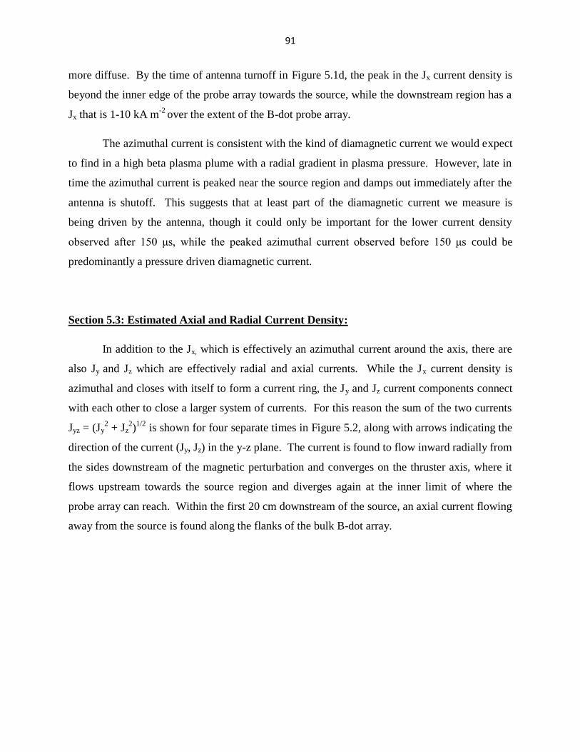
91
more diffuse. By the time of antenna turnoff in Figure 5.1d, the peak in the Jx current density is
beyond the inner edge of the probe array towards the source, while the downstream region has a
Jx that is 1-10 kA m-2
over the extent of the B-dot probe array.
The azimuthal current is consistent with the kind of diamagnetic current we would expect
to find in a high beta plasma plume with a radial gradient in plasma pressure. However, late in
time the azimuthal current is peaked near the source region and damps out immediately after the
antenna is shutoff. This suggests that at least part of the diamagnetic current we measure is
being driven by the antenna, though it could only be important for the lower current density
observed after 150 μs, while the peaked azimuthal current observed before 150 μs could be
predominantly a pressure driven diamagnetic current.
Section 5.3: Estimated Axial and Radial Current Density:
In addition to the Jx, which is effectively an azimuthal current around the axis, there are
also Jy and Jz which are effectively radial and axial currents. While the Jx current density is
azimuthal and closes with itself to form a current ring, the Jy and Jz current components connect
with each other to close a larger system of currents. For this reason the sum of the two currents
Jyz = (Jy2 + Jz
2)1/2
is shown for four separate times in Figure 5.2, along with arrows indicating the
direction of the current (Jy, Jz) in the y-z plane. The current is found to flow inward radially from
the sides downstream of the magnetic perturbation and converges on the thruster axis, where it
flows upstream towards the source region and diverges again at the inner limit of where the
probe array can reach. Within the first 20 cm downstream of the source, an axial current flowing
away from the source is found along the flanks of the bulk B-dot array.

92
Figure 5.2: Estimated Jyz Current Density and direction for four separate times. Colored
contours indicate sum of the two current componets, while arrows indicate the direction and
relative magnitude of the current. Note the color bar scale has changed from the previous figure.
Even early in time in Figure 5.2a at t = 100 μs the Jyz is only partially measured by the
probe array. Current flows out along the flanks, then converges on the axis downstream, and
finally comes back upstream along the axis to close the path: above the axis a small loop of
current can be discerned going out from the source along the edge and then converging on the
axis to return. At 20-25 cm downstream current is flowing in radially from the edge, suggesting
that the structure of currents has already expanded past the limit of the probe array. Later in time
at 125 μs in Figure 5.2b, the Jyz has propagated downstream and expanded well beyond the edges
of the probe. Rather than seeing the whole loop of the current like in the previous frame, in
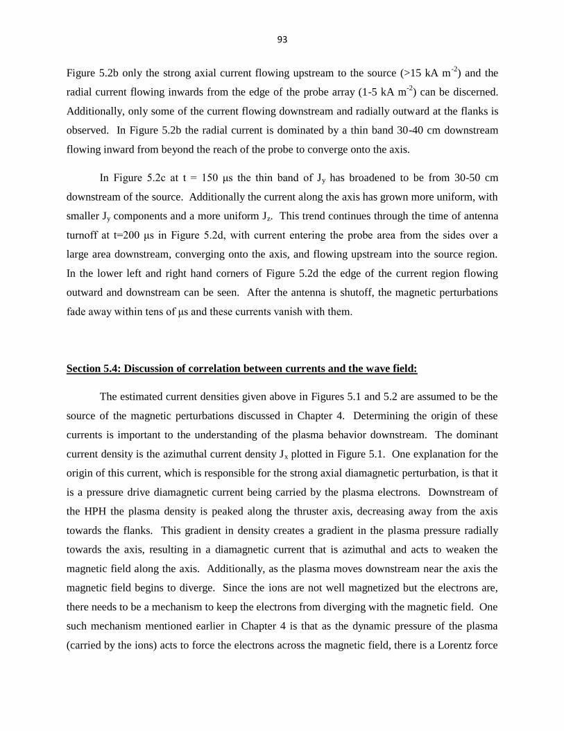
93
Figure 5.2b only the strong axial current flowing upstream to the source (>15 kA m-2
) and the
radial current flowing inwards from the edge of the probe array (1-5 kA m-2
) can be discerned.
Additionally, only some of the current flowing downstream and radially outward at the flanks is
observed. In Figure 5.2b the radial current is dominated by a thin band 30-40 cm downstream
flowing inward from beyond the reach of the probe to converge onto the axis.
In Figure 5.2c at t = 150 μs the thin band of Jy has broadened to be from 30-50 cm
downstream of the source. Additionally the current along the axis has grown more uniform, with
smaller Jy components and a more uniform Jz. This trend continues through the time of antenna
turnoff at t=200 μs in Figure 5.2d, with current entering the probe area from the sides over a
large area downstream, converging onto the axis, and flowing upstream into the source region.
In the lower left and right hand corners of Figure 5.2d the edge of the current region flowing
outward and downstream can be seen. After the antenna is shutoff, the magnetic perturbations
fade away within tens of μs and these currents vanish with them.
Section 5.4: Discussion of correlation between currents and the wave field:
The estimated current densities given above in Figures 5.1 and 5.2 are assumed to be the
source of the magnetic perturbations discussed in Chapter 4. Determining the origin of these
currents is important to the understanding of the plasma behavior downstream. The dominant
current density is the azimuthal current density Jx plotted in Figure 5.1. One explanation for the
origin of this current, which is responsible for the strong axial diamagnetic perturbation, is that it
is a pressure drive diamagnetic current being carried by the plasma electrons. Downstream of
the HPH the plasma density is peaked along the thruster axis, decreasing away from the axis
towards the flanks. This gradient in density creates a gradient in the plasma pressure radially
towards the axis, resulting in a diamagnetic current that is azimuthal and acts to weaken the
magnetic field along the axis. Additionally, as the plasma moves downstream near the axis the
magnetic field begins to diverge. Since the ions are not well magnetized but the electrons are,
there needs to be a mechanism to keep the electrons from diverging with the magnetic field. One
such mechanism mentioned earlier in Chapter 4 is that as the dynamic pressure of the plasma
(carried by the ions) acts to force the electrons across the magnetic field, there is a Lorentz force

94
that drives the electrons in an azimuthal current to weaken the magnetic field to allow the
electrons to move through. With sufficient plasma pressure (either thermal pressure or dynamic
pressure), these diamagnetic currents create a diamagnetic cavity where the ions and electrons
can flow downstream unhindered.
An alternative explanation for the origin of the azimuthal current is that it’s being directly
driven by the helicon wave propagating through the plasma. Comparing the magnitude of the
wave magnetic field along the axis in Figure 4.5 with the axial position of the azimuthal current
density in Figure 5.1, there is correlation between where the wave magnetic field falls off in
strength and the edge of the current drive region. Early in time at t=100 μs the wave magnetic
field does not extend past 20 cm, and neither does the azimuthal current ring. Later in time at
t=125 μs both have extended to ~30 cm downstream of the source. Later in time both have
extended further down the axis, falling off in magnitude the further from the source.
This wave magnetic field is perpendicular to the base magnetic field and rotates in a
right-handed fashion in time around the base magnetic field. This wave magnetic field is >10
gauss in magnitude near the source early in time and is >5 gauss as far as 20 cm downstream at
the time of peak current density in Figure 5.1. This wave magnetic field is strong enough to
magnetize the electrons (electron gyro-radius is <2 cm), so that as the magnetic field rotates in
time around the base magnetic field the electrons will be dragged along with the magnetic field.
Moving the electrons in a right-handed fashion around the magnetic field without affecting the
ions results in an azimuthal current in the direction measured in Figure 5.1. However, even if the
wave magnetic field could be driving the electrons around at the wave frequency, collisions
between the electrons and other plasma particles can interrupt this azimuthal motion. The
electron-ion collision frequency is ~900 kHz and the electron-electron collision frequency is ~1.5
MHz, which are 1.5-3 times higher than the wave frequency of ~600 kHz. This would mean that
a current being driven by the wave carrying electrons would be strongly damped by collisions.
To make a simple estimate, consider the case at t=125 µs plotted in Figure 5.1b: the
current density is peaked 2-4 cm off the axis ~20 cm downstream, and the wave magnetic field
shown in Figure 4.5 at the same time indicates that the wave field is strong enough to magnetize
the electrons at this position, but not the ions. Considering a current flowing 3 cm off axis,
carried by the plasma electrons rotating at 600 kHz. The electron density is ~3x10¹⁸
m-3
at this

95
position, so if all the electrons were rotating with the wave at the angular speed, this would give
a current density of 54 kA/m2. Since the collision rate is roughly 3 times higher than the angular
rotation rate, we can estimate that perhaps only 1/3rd
of the electrons can make it around on
average without colliding with something. Reducing the electron density carrying the current to
1x10¹⁸
m-3
yields an estimated current density of 18 kA/m2, which is roughly equal to the peak
current density at that position plotted in Figure 5.1b.
If the plasma wave is directly driving electrons in an azimuthal current at the angular
velocity of the wave rotating, then increasing or decreasing the frequency at which the wave
rotates should have a measurable effect on the plasma currents. Unfortunately, adjusting the
frequency at which the helicon wave is driven has other consequences on the ionization and
acceleration of the plasma, since it is also responsible for the generation of the plasma in the
source. The issues and results involving the changing of the antenna frequency to alter the
angular velocity of the wave will be discussed later in Chapter 7.
Section 5.5: Discussion of the meaning of axial and radial current:
In addition to the diamagnetic perturbations to the field (Bz, By) discussed in Chapter 4,
there was an additional perturbation to the field in the azimuthal direction Bx plotted in Figure
4.9. This perturbation was not diamagnetic because there was no azimuthal component to the
base magnetic field. This perturbation was directed in a left-handed fashion around the axis in
the same direction as the azimuthal current plotted in Figure 5.1. To sustain this azimuthal
magnetic field requires a current to flow both axially and radially around this region, with the
current responsible for this perturbation plotted in Figure 5.2.
If the current density in Figure 5.2 is carried by the plasma electrons, this suggests a
population of electrons moving out away from the source along the axis towards the downstream
edge of the plasma. These electrons then move out across the plasma towards the flanks at the
limit where the probe can detect them. The electrons then travel back along the flanks of the
dipole magnetic field back towards the source region to complete the loop. It was already shown
in section 5.3 that the current appears to be conserved. The peak current density along the axis in
Figure 5.2 is ~15 kA/m2, and staying within 10-20 cm downstream of the source. If this current

96
is being carried by the plasma electrons along the axis with an electron density ne~3x10¹⁸
m-3
,
then this suggests the electrons moving downstream along the axis at ~31 km/s. This velocity is
much less than the thermal speed of the electrons at Te ~ 10 eV, which is ~1,800 km/s. This
means that only a small drift of the electrons compared to their thermal motion is needed to
generate this current.
The following sections discuss the velocity of the plasma ions downstream and if the
increased diamagnetic currents result in increased acceleration of the ions.
Section 5.6: Ion velocities measured on Axis:
In Chapters 1 and 2 it was described how the wave driven by the high power helicon is at
a frequency well above the ion cyclotron frequency and well below that of the electron cyclotron
frequency. This allows the helicon antenna to directly affect the electrons while the ions are
relatively motionless. To maintain quasi-neutrality, as the electrons are accelerated downstream
of the HPH an ambipolar electric field develops that accelerates the ions to move downstream at
the expense of the electron energy. These ions are not well magnetized, and once accelerated
downstream they move across the magnetic field with little to no deflection while the electrons
need several mechanisms to move across the magnetic field to keep up with them (as described
in Chapter 4). Measuring the velocity of these heavy, directed ions is a useful diagnostic to
study the plasma characteristics downstream of the HPH source.
Two experimental methods were used to measure the downstream velocity of the plasma.
The first was using pairs of langmuir probes to make time-of-flight estimates of the velocity of
the plasma. By comparing the difference in time between the peak plasma densities measured at
two different probes downstream, an estimate of the bulk velocity of the plasma could be
obtained. Previous work on HPH by Prager [2] used this method to estimate the bulk flow
velocity at 8-9 km/s. More recent time of flight estimates taken as part of this research also
indicated a bulk speed of 8-11 km/s at similar input power levels. This was based on
measurements of the plasma density at 3 downstream locations with floating double-langmuir
probes as described in chapter 3. This langmuir data is shown below in Figure 5.3.

97
Figure 5.3: Plasma density as a function of time on axis for three locations downstream of HPH.
The difference in time between the peaks is used to estimate the bulk speed of the plasma.
The time of flight method for estimating the ion velocity is most applicable when the ion
population is moving together at close the same speed and does not speed up or slow down
between the langmuir probes. This makes it less useful for measuring the ion speeds
downstream of HPH because it has been shown in previous work by Ziemba [9] and Prager [2]
that the ion population is increasing in speed downstream of the source and so it is likely that the
velocity would not have been constant between the two probes. Since the langmuir probe data is
taken with the probe in saturation, it is measuring ions with a range of energies and displaying
the total current received, even though the ions that contributed to the peak signal in the first
curve of Figure 5.3 are not necessarily the same ions which generated the peak signal in the third
curve of Figure 5.3.
The second experimental method of measuring the downstream plasma velocity
addresses this problem by measuring the kinetic energy of the plasma particles using a retarding
field energy analyzer (RFA) as described in Chapter 3. The RFA measures the ion energies
Time of Flight via Langmuir
2.69E-04
3.24E-04
3.39E-04
-2.00E-03
0.00E+00
2.00E-03
4.00E-03
6.00E-03
8.00E-03
1.00E-02
1.20E-02
1.40E-02
1.00E-04 1.50E-04 2.00E-04 2.50E-04 3.00E-04 3.50E-04 4.00E-04 4.50E-04 5.00E-04
Time (s)
Lan
gm
uir
Cu
rren
t (a
rb u
nit
s)
63 cm
109 cm
135 cm

98
along the axis of the detector, which is typically aligned with the thruster axis to measure the
directed energy of the ions downstream of the source along the axis. As the potential on the
retarding grid is raised, fewer ions in the plasma have enough energy to get through the device to
the collected plate at the rear of the detector. By taking the derivative of the ion current to the
collector as a function of retarding potential voltage, we can measure the ion energy distribution
function parallel to the axis (and the magnetic field). If we also assume that the ions striking the
plate are all singly ionized argon, the directed energy along the axis of the ions can be converted
to a measure of ion velocity into the detector using equation 5.4:
i
RFAion
m
Ev
2 (5.4)
where vion is the estimated ion directed velocity, ERFA is the energy of the ion as measured by the
RFA in electron-volts, and mi is the mass of the argon ions.
One possible complication with making this measurement is if the ions are accelerated
relative to the detector so that the measured velocity given by the RFA is not the same as the
flow velocity of the ions. This could be caused by the plasma forming a sheath around the probe
(as described in chapter 3) that acts to accelerate ions towards the grounded chassis of the RFA.
This would increase the measured energies of the ions by an amount roughly equal to plasma
potential between the flowing plasma and ground. It would also have the effect of accelerating
ions into the detector along the sides of the RFA, and if the potential difference is larger than the
directed energy of some of the ions, even backwards into the rear of the RFA. This population of
ions has been observed in measurements by Charles et al [23] in their system and was used as an
estimate of the plasma potential. This effect is not observed in the plume downstream of HPH,
as observed by Prager et al [10]. This was determined by rotating the RFA input orifice relative
to the thruster axis and measuring the decrease of ions entering the source as the angle between
them increased. Once the RFA detector orifice was perpendicular to the output of the HPH
thruster, the measured ion current dropped to zero, which should not have occurred if there was a
population of ions being accelerated into the RFA by a plasma sheath. Measurements of the ion
speed by the time of flight method mentioned earlier also roughly matched the velocities

99
measured by the ion energy distribution, making it unlikely that the measured ion energies were
significantly altered from what they were in the plasma plume.
For the two magnetic field configurations discussed in chapter 4, one with the wave
propagating parallel and the other anti-parallel, there is a significant difference in the ion velocity
distribution function (IVDF) when the wave propagation is parallel and the large diamagnetic
perturbation is observed. In Figure 5.4, the two cases are compared for six different times and
the IVDF is presented as measured 60 cm downstream of the source along the thruster axis:

100
Figure 5.4: Ion velocities on axis 60 cm downstream of the HPH with two different magnetic
field configurations previously mentioned in chapter 4. The configuration with magnetic field
parallel to the wave vector k is associated with large diamagnetic perturbations and is correlated
with a significant increase in the population of fast ions. The red trace was measuring a smaller
population of ions and there is a larger margin of error in the shape of this distribution.
In the first panel of Figure 5.4, which represents the early in time population from the
source to arrive 60 cm downstream, there are significantly more of the fast ions present in the

101
parallel propagation case than the anti-parallel case. Additionally, the ions of the parallel
propagation case are ~2 km/s faster than the anti-parallel case. Over the next 50 μs in the
subsequent two panels of Figure 5.4 the IVDF of both cases shifts to lower velocities while the
magnitude increases, possibly a result of slower ions arriving later or changes in how the ions are
being accelerated both in the source region and downstream. In both panels the IVDF of the
parallel case has an increased number of ions over the energy range compared to the anti-parallel
case, as well a slightly faster population of ions present in the parallel case but not the other. In
the final three panels of Figure 5.4 the number of ions measured in the parallel case decreases but
maintains a relatively high velocity, while the anti-parallel case has a slower decrease in ion
number but a decrease in velocity of ~2-3 km/s. This set of data suggests that there is a
mechanism that is accelerating ions in the parallel case that is weakened or absent in the anti-
parallel case.
Section 5.7: Discussion of when the ions begin moving super-sonic and super-Alfvenic:
The measurements of ion velocity through time of flight estimates and the RFA in the
previous section were both made further than 60 cm downstream of the source region. Previous
measurements by Prager et Al [10] with the RFA indicated that at 20 cm downstream of the
source the peak of the ion population had a velocity of ~6.5 km/s early in time which increased
to ~8.5 km/s by the time the source antenna was shut off. When the same detector was moved to
50 cm downstream, it measured the velocity of the peak of the ion population to be ~10.9 km/s
early in time and ~10.2 km/s when the antenna was shut off. This suggests that more than 50%
of the acceleration of the ions is occurring within the first 20 cm of the source region, but that
there is still a mechanism accelerating the ions between 20 cm and 50 cm downstream by as
much as 1-4 km/s at different times [10].
As the ion velocity increases beyond the sound speed of the plasma or the alfven speed,
the behavior of the downstream plasma can change. The sound speed of the plasma is given by
[3]:

102
i
iie
sm
kTkTv
(5.5)
where Te and Ti are the electron and ion temperatures respectively, γi for the ions is ~5/3, and mi
is the mass of the ions. This is the speed at which ion acoustic waves can travel through the
plasma. For electron temperatures of ~10 eV and assuming Ti~0 (cold ions), this gives a sound
speed of ~4.9 km/s for the downstream plasma. For an ion temperature of 1-2 eV, the sounds
speed increases to 5-6 km/s, and for 10 eV ions the sound speed is ~8 km/s. In the case of HPH,
the ion temperature was measured to be at most 1-2 eV in the previous work by Prager [2], so the
ions are expected to be colder than the electrons and the sound speed to be 5-6 km/s. Based on
the velocity measurements from the time of flight probes, the plasma bulk speed is comparable
or higher than the sound speed of the plasma. The RFA measurements also indicate that the
plasma is flowing faster than the sound speed with 20 cm of the source exit [10]. Comparing the
directed ion speed to the sound speed of the plasma gives the Mach number of the plasma, but it
is more convenient in equation 5.6 to consider the square of the Mach number:
iie
i
iie
ii
s
i
skTkT
E
kTkT
vm
v
vM
22
2
2
2
(5.6)
where Ms is the Mach number and Ei is the directed energy of the ions as measured by the RFA.
It’s convenient to use the square of the Mach number because as the directed energy of the ions
becomes greater than half the thermal energy of the plasma particles, it is clear that the Mach
number will be greater than 1 and the flow will transition to super-sonic. The directed energy of
the ions is the plasma property measured by the RFA.
The Alfven speed of the plasma is given by [3]:
ii
Amn
Bv
0
(5.7)
where B is the magnetic field strength, and ni and mi are the density and mass of the ion
population. Typically the B used in this calculation for laboratory plasmas is the strength of the

103
background magnetic field without adding the modifications to the magnetic field by the plasma
particles. In the case of HPH where there is a significant diamagnetic decrease in the field, this
would result in a local decrease in the Alfven speed, so the Alfven speed being considered here
(using the unmodified B0) will be an upper limit to the speed. The Alfven speed will also be
changing as a function of time as the plasma flows downstream and the ion density varies.
Comparing the directed ion speed to the Alfven speed yields the Alfven Mach number of the
plasma, but again it is more convenient in equation 5.8 to consider the square of the Alfven
Mach number:
0
2
2
i
0
2
2
i
2
2
2
21
B
vmn
B
vmn
v
vM
iiii
a
ia (5.8)
where Ma is the Alfven Mach number. It is convenient to use the square of the Alfven Mach
number because then equation 5.8 indicates that as the directed energy density of the ions begins
to exceed the magnetic energy density of the background field, the plasma is expected to
transition to a super-Alfvenic regime. This ratio of particle energy density to magnetic energy
density is similar to the measure of plasma Beta which considers the ratio between thermal
energy density of the plasma electrons and magnetic energy density, or alternatively the electron
pressure compared to the magnetic pressure. Equation 5.8 considers a dynamic pressure of the
ions flowing downstream compared to the magnetic pressure, and can also be referred to as the
dynamic plasma beta [7].
The background plasma population varies with time and position downstream of HPH,
and the following three figures illustrate the change in Alfven speed and the balance between
electron energy and magnetic energy (plasma beta) along the source axis. These plots
correspond to the case from Figure 5.4 when the wave vector was parallel with the magnetic
field and there was a strong diamagnetic signal with a faster ion population. Figure 5.5 plots the
energy density of the electrons, energy density of the magnetic field, and the calculated Alfven
speed of the plasma along the axis for time early into the shot before the bulk of the plasma has
moved far downstream. At this time the energy in the electrons downstream has risen to the
point where they have comparable energy to the background field from about 20 cm downstream

104
of the source and beyond. The Alfven speed is 10-12 km/s immediately downstream of the
source, but as the field decreases in strength it becomes ~5 km/s. This early in time when there
no significant plasma far downstream of the source the Alfven speed does not continue to
decrease with distance from the source as the plasma density is low, but this is not the case for
the rest of the shot.
Figure 5.5: Comparison of the energy density of the electrons and the magnetic field downstream
of the source along the axis at 91 µs, along with the estimated Alfven Speed. The energy
densities are plotted along the left axis in units of Joules per cubic meter, while the Alfven speed
is plotted along the right axis in km/s.
The ion velocity measured at 60 cm downstream of the source in Figure 5.4 indicated the
ion peak flowing with a velocity of 12-14 km/s at approximately this time, so that far
downstream the plasma flow is super-Alfvenic and super-sonic. If the bulk of the ion
acceleration or all of it is occurring in or close to the source region early in time, then the fast
ions measured downstream could be super-Alfvenic within 10 cm of the source region.
Most Probable Ion Speed
(Downstream at RFA)
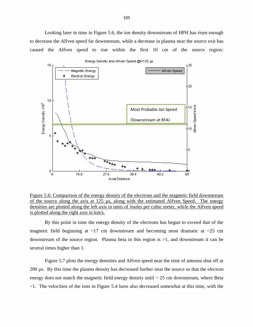
105
Looking later in time in Figure 5.6, the ion density downstream of HPH has risen enough
to decrease the Alfven speed far downstream, while a decrease in plasma near the source exit has
caused the Alfven speed to rise within the first 10 cm of the source region:
Figure 5.6: Comparison of the energy density of the electrons and the magnetic field downstream
of the source along the axis at 125 µs, along with the estimated Alfven Speed. The energy
densities are plotted along the left axis in units of Joules per cubic meter, while the Alfven speed
is plotted along the right axis in km/s.
By this point in time the energy density of the electrons has begun to exceed that of the
magnetic field beginning at ~17 cm downstream and becoming most dramatic at ~25 cm
downstream of the source region. Plasma beta in this region is >1, and downstream it can be
several times higher than 1.
Figure 5.7 plots the energy densities and Alfven speed near the time of antenna shut off at
200 µs. By this time the plasma density has decreased further near the source so that the electron
energy does not match the magnetic field energy density until ~ 25 cm downstream, where Beta
~1. The velocities of the ions in Figure 5.4 have also decreased somewhat at this time, with the
Most Probable Ion Speed
(Downstream at RFA)
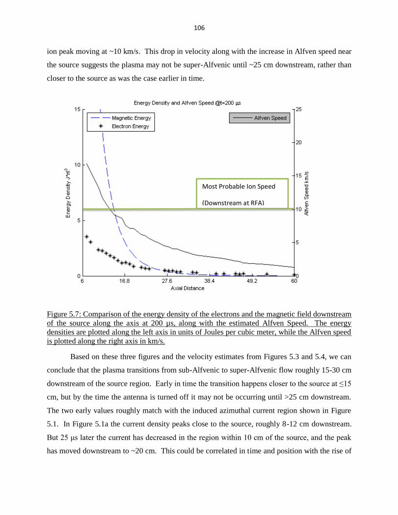
106
ion peak moving at ~10 km/s. This drop in velocity along with the increase in Alfven speed near
the source suggests the plasma may not be super-Alfvenic until ~25 cm downstream, rather than
closer to the source as was the case earlier in time.
Figure 5.7: Comparison of the energy density of the electrons and the magnetic field downstream
of the source along the axis at 200 µs, along with the estimated Alfven Speed. The energy
densities are plotted along the left axis in units of Joules per cubic meter, while the Alfven speed
is plotted along the right axis in km/s.
Based on these three figures and the velocity estimates from Figures 5.3 and 5.4, we can
conclude that the plasma transitions from sub-Alfvenic to super-Alfvenic flow roughly 15-30 cm
downstream of the source region. Early in time the transition happens closer to the source at ≤15
cm, but by the time the antenna is turned off it may not be occurring until >25 cm downstream.
The two early values roughly match with the induced azimuthal current region shown in Figure
5.1. In Figure 5.1a the current density peaks close to the source, roughly 8-12 cm downstream.
But 25 μs later the current has decreased in the region within 10 cm of the source, and the peak
has moved downstream to ~20 cm. This could be correlated in time and position with the rise of
Most Probable Ion Speed
(Downstream at RFA)

107
the Alfven speed near the source region. The region where the transition to super-Alfvenic flow
is estimated to occur also correlates in position and time with the region along the axis where
plasma beta ≥ 1 near the source region.
This discussion of the Alfven speed has been limited to the data set in Figure 5.4 where
the wave number ‘k’ is parallel with B0. In the other case, where ‘k’ is anti-parallel to B0, the
ions are significantly slower later in time. In the anti-parallel case the diamagnetic perturbation
to the field is significantly smaller, and measured induced currents are also smaller. This
correlation between the increase in ion velocity and the presence of large diamagnetic currents,
together in the region where the plasma is thought to be transitioning into super-sonic and super-
Alfvenic flow, suggests that it could be responsible for the acceleration of the plasma
downstream of the source.
Section 5.8: Estimated Acceleration by JxB Forces:
When there are currents flowing in a plasma perpendicular to the magnetic field, there is
a Lorentz force on the plasma particles carrying the current given by:
JxBF (5.9)
where F is the force density in N/m3, J is the current density in A/m
2, and B is the magnetic field
in tesla. This force acts both on the ions and electrons in the plasma even if the bulk of the
current is being carried by the electron motion, so the energization of the plasma is usually
determined by the force on the much heavier ions.
A different plasma thruster concept known as “Faraday Acceleration with Radio-
Frequency Assisted Discharge” or FARAD proposed by Choueiri et Al [26] uses a helicon
plasma source to generate plasma downstream that is then accelerated by a large azimuthal
current induced by a separate coil for a pulse roughly 1-2 μs long. The azimuthal current is
across a radial magnetic field of several hundred gauss and results in an axial acceleration of the
plasma (in the form of a moving plasma sheet). In their initial results, the inductive coil
downstream was pulsed with 20 kA of current, which induced a current density in the plasma

108
roughly 1 MA/m2 and was combined with an induced radial magnetic field of ~600 gauss (.06
T). This force acted on argon plasma that had a density of ~1020
m-3
for roughly 1μs, leading to
an estimated acceleration of ~1 km/s. Choueiri et Al [26] suggest that perhaps not all of the
plasma is picked up and accelerated by the current sheet, leading to a less dense volume of
plasma accelerated to a higher velocity.
Downstream of the HPH there is also an azimuthal current being driven, which was
plotted as a function of position near the source axis in Figure 5.1. The current downstream of
HPH peaks at 20 kA/m2, which is two orders of magnitude lower than that driven by the FARAD
inductive coil, but the current is driven for a significantly longer time of more than 100 μs.
Another key difference is that the inductive coil of FARAD induces a strong radial magnetic
field of ~600 gauss, with the axial magnetic field approximately zero. The magnetic field
immediately downstream of HPH near the axis is mostly an axial magnetic field on the order of
100 gauss, with a much smaller radial component. This means the JxB acceleration downstream
of HPH not only has an axial component, but also a radial component as well. The radial
component of the JxB force is the y component, and is plotted for four times downstream of the
source in Figure 5.8.
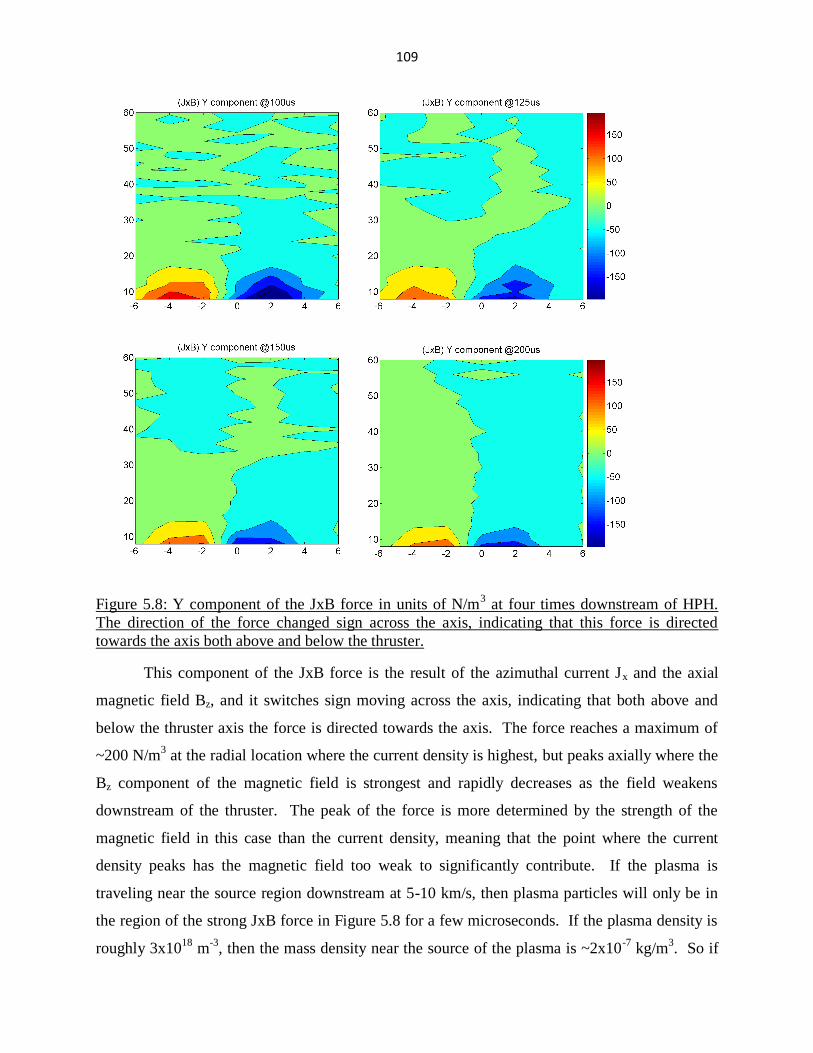
109
Figure 5.8: Y component of the JxB force in units of N/m3 at four times downstream of HPH.
The direction of the force changed sign across the axis, indicating that this force is directed
towards the axis both above and below the thruster.
This component of the JxB force is the result of the azimuthal current Jx and the axial
magnetic field Bz, and it switches sign moving across the axis, indicating that both above and
below the thruster axis the force is directed towards the axis. The force reaches a maximum of
~200 N/m3 at the radial location where the current density is highest, but peaks axially where the
Bz component of the magnetic field is strongest and rapidly decreases as the field weakens
downstream of the thruster. The peak of the force is more determined by the strength of the
magnetic field in this case than the current density, meaning that the point where the current
density peaks has the magnetic field too weak to significantly contribute. If the plasma is
traveling near the source region downstream at 5-10 km/s, then plasma particles will only be in
the region of the strong JxB force in Figure 5.8 for a few microseconds. If the plasma density is
roughly 3x10¹⁸
m-3
, then the mass density near the source of the plasma is ~2x10⁻⁷
kg/m3. So if

110
the plasma is acted on by a 200 N/m3 force for ~4 μs at a mass density of 2x10
-7 kg/m
3, then the
estimated acceleration towards the axis is roughly 4 km/s. This acceleration towards the axis
near the source region should have a significant effect on the plasma ions, forcing them onto the
thruster axis.
The axial component of the JxB force is the result of the strong azimuthal current Jx
interacting with the relatively weak radial magnetic field By near the thruster axis. This Z
component of the JxB force is plotted for four times in Figure 5.9.
Figure 5.9: Z component of the JxB force in units of N/m3 at four times downstream of HPH.
The force is directed downstream away from HPH. Note the change in color bar scale from
previous figure.
The JxB force directed axially downstream of HPH plotted in Figure 5.9 is significantly
weaker than the force directed towards the axis in the previous figure. The peak force is roughly
50 N/m3, down by about a factor of 4 from the peak radial force. By making a similar estimate
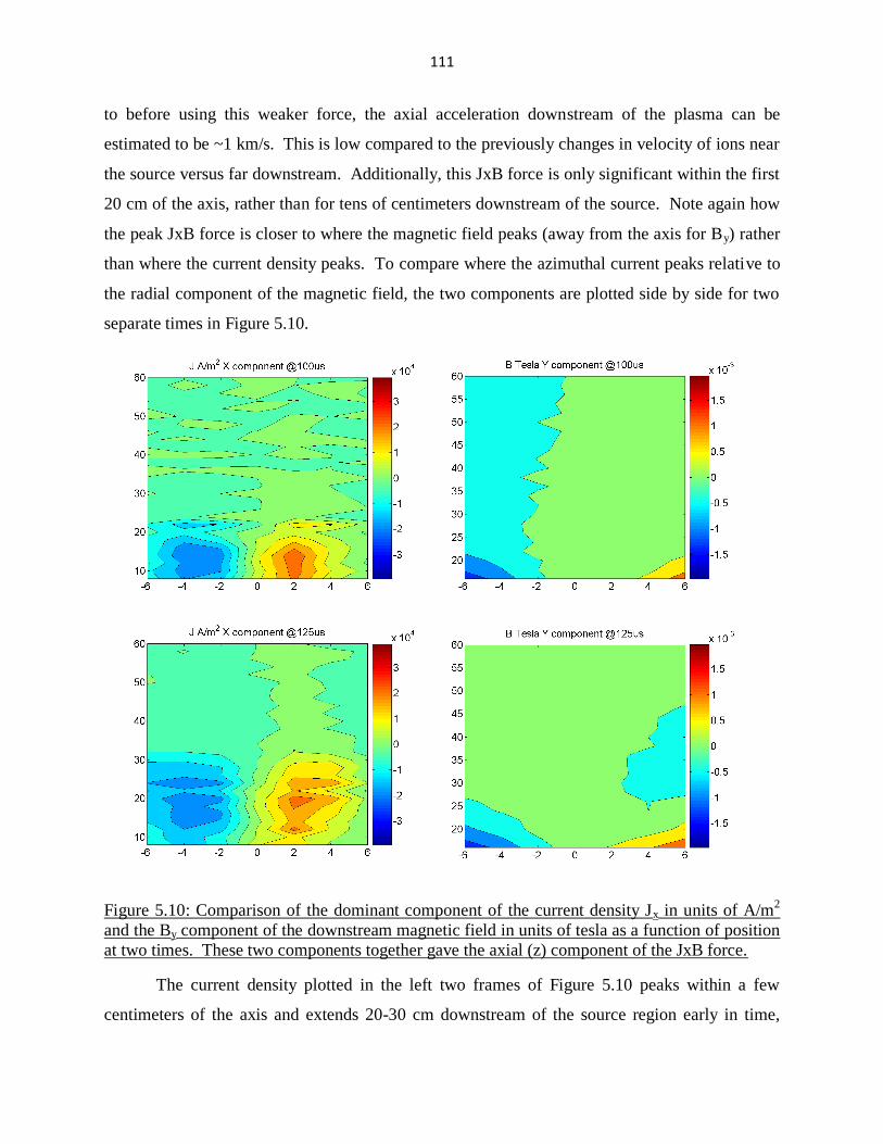
111
to before using this weaker force, the axial acceleration downstream of the plasma can be
estimated to be ~1 km/s. This is low compared to the previously changes in velocity of ions near
the source versus far downstream. Additionally, this JxB force is only significant within the first
20 cm of the axis, rather than for tens of centimeters downstream of the source. Note again how
the peak JxB force is closer to where the magnetic field peaks (away from the axis for By) rather
than where the current density peaks. To compare where the azimuthal current peaks relative to
the radial component of the magnetic field, the two components are plotted side by side for two
separate times in Figure 5.10.
Figure 5.10: Comparison of the dominant component of the current density Jx in units of A/m2
and the By component of the downstream magnetic field in units of tesla as a function of position
at two times. These two components together gave the axial (z) component of the JxB force.
The current density plotted in the left two frames of Figure 5.10 peaks within a few
centimeters of the axis and extends 20-30 cm downstream of the source region early in time,

112
while the radial component of the magnetic field is low near the axis and only begins to become
significant more than 5 cm from the axis even close to the source region. The JxB force plotted
above in Figure 5.9 is the result of the weaker regions of the current density interacting with the
weaker regions of radial magnetic field since there’s no real overlap between the two peaks. Part
of the reason for this is that the diamagnetic perturbation described in chapter 4 weakens the
radial component of the magnetic field near the axis.
If the JxB force is the acceleration mechanism responsible for the downstream
acceleration of the plasma, it’s possible that the weaker force is not accelerating the bulk of the
plasma and instead only a fraction of it as proposed for the FARAD experiment [26]. It’s also
possible that some of the radial acceleration near the source forces enough plasma onto the axis
that the increase in plasma pressure ends up accelerating the plasma along the axis further
downstream since there’s nothing to contain the plasma on the other end. The JxB results
presented here suggest that it was a lack of magnetic field density overlapping the region where
the current density was highest that was preventing the JxB force from becoming more
significant. Chapter 6 presents results from modifying the downstream magnetic field with
magnetic nozzles and the effect this has on the downstream ion velocities.

113
Chapter 6: Effect of Magnetic Nozzles Downstream of HPH
Section 6.1: Increasing the Magnetic Field Downstream of the Source
The base magnetic field generated by the coils around the source region decreases like a
dipole downstream of the source, falling to a few gauss within 50 cm and becoming dominated
by the Earth’s magnetic field within 150 cm. Increasing the magnetic field downstream of the
source region by placing additional magnet coils downstream of the source region along the
thruster axis is expected to have several effects on the plasma flow. The primary effect is to act
on the plasma like a magnetic nozzle, focusing the plasma outflow and increasing the electron
density near the axis. This will slow the thermal expansion of the plasma due to the electron
temperature and extend the region where the plasma is near the axis and continues to be
accelerated by the interaction with the source region. Additional effects will include changing
the Alfven speed and the position downstream where the plasma detaches from the magnetic
field.
Lastly, the increased magnetic field will increase the electron gyro-frequency relative to
the electron collision rate, resulting in more strongly magnetized electrons. The ambipolar
electric fields that develop between the electrons and the colder ions may change how the ions
are accelerated downstream of the source region and affect the measured ion velocities. It is also
expected that the increased magnetic field downstream of the source may affect the generation of
JxB forces that were discussed in Chapter 5. While the electrons are expected to be magnetized
downstream of the source with the increased magnetic field, the same is not necessarily true of
the ions.
In Chapter 4 it was described how downstream of the source (without additional magnet
coils) the ions were not expected to be well magnetized. In order for the ions to be well
magnetized downstream of the source, several conditions needed to be satisfied: the ions would
need to be able to gyrate several times within the plasma without hitting the walls or leaving the
plasm, the ion gyro-radius needed to be less than or equal to the scale length of the magnetic
field in order for the field to be relatively uniform over the course of a gyro-orbit, and the
114
collision frequency for the ions needed to be lower than the ion gyro-frequency. The difficulty
that arises is that in the regions where the magnetic field is strong enough to satisfy the first
condition, the plasma density is typically high enough for the second condition to be violated.
To compare the magnitudes involved, the first condition depends on the ion gyro-radius given by
[17]:
√
√
√
6.1
where rci is given in centimeters, Ti is the ion temperature in eV and B is the magnetic field
magnitude in gauss. If the magnetic field downstream is only a few gauss, then for even
reasonably cold ions of ~1 eV the gyro-radius of the ions will be on the scale of meters, which is
on the same order as the chamber diameter. This would suggest that even for cold ions, weak
magnetic fields would not result in magnetized ions because they would collide with the chamber
wall before completing a gyro-orbit. If the magnetic field is raised downstream to be on the
order of ~100 gauss, then for reasonably cold ions of ~1 eV the gyro-radius would be < 10 cm.
This suggests that for ions not much warmer than 1 eV, a magnetic field on the order of 100
gauss would keep the gyro-orbit small enough compared to the radius of the magnets generating
the field that the first condition could be satisfied.
To consider the magnitudes involved for the second condition, the ion gyro-frequency
downstream of the source is given by [17]:
6.2
where B is the magnetic field strength in gauss. So for a downstream magnetic field on the order
of 100 gauss that could satisfy the first condition, the ion gyro-frequency will be on the order of
~3.8 kHz. The second condition will be satisfied if this gyro-frequency is larger than the ion
collision frequency given by [17]:
√
6.3
where ln(λ) for normal cold plasma laboratory conditions can be approximated as 10 and ni is the
ion density per cubic centimeter. For the case given above where the gyro-frequency is ~3.8 kHz

115
and the ion temperature is ~1 eV, in order to satisfy the second condition the ion density must be
less than 5x10¹⁰
cm-3
. This is unrealistic because even without any downstream modification to
the base field the plasma density downstream of the source was on the order of 1011
-1012
cm-3
,
and data taken with a field increase to ~100 gauss as described had a density on the order of 1013
cm-3
in that region (this data is presented below in section 6.x). Increasing the ion temperature
can lower the coulomb collision frequency between the ions, but in order to make up for the 3
orders of magnitude difference the increase in temperature has to be dramatic, far more than is
realistic given the estimates of ion temperature parallel to the magnetic field made by Prager [2].
The modification of the magnetic field downstream by adding a subsequent coil was
made to observe some of the effects listed above and their subsequent effect on the exhaust
velocity of the plasma outflow. The intention of the magnetic coils is for it to affect the plasma
as a magnetic nozzle, shaping the plasma outflow to result in a faster and more directed plasma
plume. In this chapter these additional magnetic coils will be referred to as nozzles for this
reason.
Section 6.2: Plasma flow in a converging magnetic nozzle.
For a conventional fluid nozzle of the Laval type, the nozzle is shaped to have three
distinct regions: a converging section where the decreasing cross section causes the fluid to
increase in flow speed to conserve flux, a throat section where the choked flow of the fluid
transitions from sub-sonic to trans-sonic flow, and a diverging section where the super-sonic
fluid accelerates away from the nozzle [1]. In each section the fluid flow velocity is increasing at
the expense of the thermal energy of the fluid. When considering plasma flow in a magnetic
nozzle instead of neutral flow into a physically constricting nozzle, it is not necessarily true that
the velocity of the plasma will increase going into the converging section of the magnetic nozzle.
This will depend on the degree of magnetization of the plasma particles. In the case of HPH and
many other helicon experiments the electrons are well magnetized and slow down to conserve
magnetic moment (as described below). If the ions are also magnetized, they will slow down as
well. If the ions are not well magnetized such as in the case of HPH, instead of slowing to
116
conserve magnetic moment the ion velocity is determined by the electric potential established by
the electrons.
In the case of a converging magnetic field, as the plasma particles move into the
increasing magnetic field the gyro-motion of the particles will increase at the expense of the
parallel motion of the particles as they act to conserve their magnetic moment, given by [20]:
6.4
where v⊥ is the velocity of the particle perpendicular to the magnetic field. As the magnetic field
increases, the gyro-motion of the particle will increase to keep the magnetic flux contained
within the particle’s path conserved. This increase in perpendicular velocity comes at the
expense of parallel velocity for the energy of the particle to be conserved, so as it gyrates around
the field faster it slows in its parallel motion along the magnetic field [20].
This would suggest that for a converging magnetic nozzle with magnetized electrons and
ions both, the plasma flow would slow down as it enters the converging magnetic field and the
individual particles act to conserve magnetic moment. There is some experimental confirmation
of this in the work by Inutake et Al [27] in adding a magnetic nozzle shaped to be similar to a
Laval nozzle downstream of a magneto-plasma dynamic thruster. In their results the axial flow
in the converging region was decreased compared to the case without the magnetic nozzle, while
the axial flow downstream of the nozzle was increased relative to the non-nozzle case [27].
A separate case is treated by Arefiev et Al [28] which considered cold, un-magnetized
ions and magnetized electrons in a converging magnetic nozzle field. In their model the ions
were cold and began at rest, while the electron temperature was comparable to that of laboratory
plasmas and high enough so that the converging field is not a magnetic bottle. The electrons
entering the converging magnetic field were slowed by conservation of magnetic moment as well
as being slowed as they moved away from the ions. This established an electric potential that
accelerated the ions into the converging magnetic nozzle field, increasing in ion velocity until the
sound speed was reached at roughly the throat of the nozzle. While some of the electrons did not
have enough parallel energy to pass through the magnetic nozzle, most did and continue to
establish the ambipolar electric field on the diverging side of the magnetic nozzle. In this region,

117
the electrons are accelerated away from the magnetic nozzle in the diverging field to conserve
magnetic moment, increasing the ambipolar electric potential and accelerating the ions above the
sound speed of the plasma. In this case, the ions passing through the nozzle are not slowed by
the nozzle, but instead are increasing in velocity all the way through the nozzle [28].
The model developed by Arefiev et Al [28] assumed that the electron and ion
temperatures were isotropic in the converging magnetic field region and the ions were
accelerated only up to the ion sound speed which was determined by the electron temperature as
described before in Chapter 5. In a separate treatment by Saka [29] that does not require the
plasma to be isotropic, the critical flow speed to which the ions can be accelerated by the
ambipolar electric field of the electrons in the converging magnetic field is dependent on the
ratio between the pressure of the plasma parallel and perpendicular to the magnetic field. For
conditions where the parallel pressure of the plasma flow dominates over the perpendicular
pressure (discussed in Chapter 5 as being super-Alfvenic), the critical flow speed exceeds the ion
sound speed by as much as 2-3 times and the ions can continue to be accelerated to super-sonic
speeds even in the converging region of the magnetic field [29].
These two models together suggest that in the case of HPH with its cold, unmagnetized
ions and strongly directed plasma flow, the ambipolar acceleration of the ions by the electrons
can still transition to a super-sonic flow speed even if the magnetic field is modified with a
magnetic nozzle to have a converging magnetic field geometry. As long as the electrons have
enough parallel energy to move through the magnetic nozzles without being turned back, they
can continue to cool and slow down while accelerating the plasma ions even well downstream of
the source. If there was no additional energy being added to the electrons by the antenna being
on, the electrons would lose the bulk of their thermal velocity accelerating the ions and have a
cold temperature similar to the ions. If the antenna can continue to heat the electrons
downstream of the source, this can keep the electron temperature warmer for longer and continue
to accelerate the ions to a higher directed energy.
Section 6.3 Acceleration of the plasma in a diverging magnetic field:

118
On the other side of the magnetic nozzle where the field begins to diverge again, it is
expected that the plasma flow will increase in speed. This is the result of conservation of
magnetic moment for the electrons increasing their parallel velocity, which through the
ambipolar electric field accelerates the ions. To the extent that the ions are magnetized, they will
also be sped up by conservation of magnetic moment in the diverging region of the magnetic
field [28]. The acceleration and detachment of the plasma from a diverging magnetic field has
been studied in several different models such as by Arefiev et Al [28] and Little et Al [30], and
while the specific mechanism is not determined by these models it is expected to behave in the
case of HPH as a combination of the detachment mechanisms described earlier in Chapter 4.
An additional consideration is the effect of the converging and diverging magnetic field
on azimuthal diamagnetic currents such as those measured in the previous chapters. In the case
of the converging magnetic field, the diamagnetic current with the radially inward magnetic field
generates a JxB force that is anti-parallel with the axis and is expected to slow the flow of
plasma. In the diverging field the JxB force with the radially diverging magnetic field is directed
parallel with the axis and is expected to accelerate the plasma flow downstream [27]. This
means that depending on where the currents are being driven, the introduction of a magnetic
nozzle downstream could result in speeding up or slowing down the plasma outflow as a result of
this JxB force.
Section 6.4: Introduction of a single magnetic nozzle downstream
The diamagnetic signal described in Chapter 4 peaked ~25 cm downstream. This
position was also roughly one wavelength downstream of the source region. To determine
whether this peak in the diamagnetic signal was correlated with the magnitude of the background
magnetic field at that position, a magnetic nozzle was added to increase the field 25 cm
downstream to ~100 gauss in magnitude. This nozzle was 11 cm wide and 26 cm in diameter,
positioned with its center at 25 cm downstream of the quartz face where the previously measured
diamagnetic signal peaked. This is also the position where it was expected that the plasma was
transitioning from sub-Alfvenic to super-Alfvenic flow as described in Chaper 5. The axial

119
component of the magnetic field in this new configuration is compared to the previous magnetic
field configuration in Figure 6.1.
Figure 6.1: Modification to the axial magnetic field with a nozzle positioned downstream,
centered 25 cm from the end of the source region.
The magnetic field in the source region is not significantly affected, so that the plasma
production in the source region was similar in both configurations. The magnetic field strength
falls off slower downstream of the magnetic nozzle as a result of the larger magnet radius for the
nozzle as compared to the base magnet coils. A side view of the magnetic field geometry is
plotted in Figure 6.2

120
Figure 6.2: Magnetic Field configuration with a single nozzle downstream together with Earth’s
magnetic field. The magnetic field from the source region diverges for a short distance before
entering the nozzle, and then diverges downstream before joining with the Earth’s field.
The side-view of Figure 6.2 shows the magnetic field diverging briefly as it leaves the
source region before converging again into the magnetic nozzle. Downstream of the magnetic
nozzle the field widens up and connects with the Earth’s magnetic field roughly 1.5 m
downstream of the source region. The introduction of the magnetic nozzle had a significant
effect on the collimation of the plasma, the exhaust speed of the ions, and the diamagnetic
perturbation of the magnetic field. These effects are described in the following sections.
Section 6.5: Collimation of the plasma beam with a single magnetic nozzle:
With the increased magnetic field along the axis downstream, the magnetic pressure of
the background field was increased and this resulted in more plasma close to the axis. The

121
electron density along the axis after the plasma has reached far downstream (~100 µs) is plotted
in Figure 6.3, along with the electron density from the non-nozzle case for comparison. Near the
source region where the field modification is minimal the densities are comparable, it is mainly
in the region downstream of the source surrounding the nozzle position at 25 cm and further that
are strongly affected.
Figure 6.3: Comparison of the electron density as a function of distance from the source with and
without the nozzle, showing increased plasma density on the axis.
In the non-nozzle case, the plasma density 25 cm downstream where the diamagnetic
effect was strongest was ~3x10¹⁸
m-3
, while in the nozzle case the plasma density is ~1x10¹⁹
m-3
that distance downstream, and doesn’t decrease into the low 1018
range until far downstream.
Since the input power in the source region, magnetic field, and neutral gas profiles are
unchanged the total plasma output of the source is unchanged, and this increase in density is
coming from an improved collimation of the beam. This collimation of the beam is measured
with a radial density profile, a Langmuir probe positioned 10 cm downstream and between the
source and nozzle, and displayed for four separate times in Figure 6.4. The first panel of Figure
6.4 shows a broader distribution early in time while the plasma density is still increasing at 10
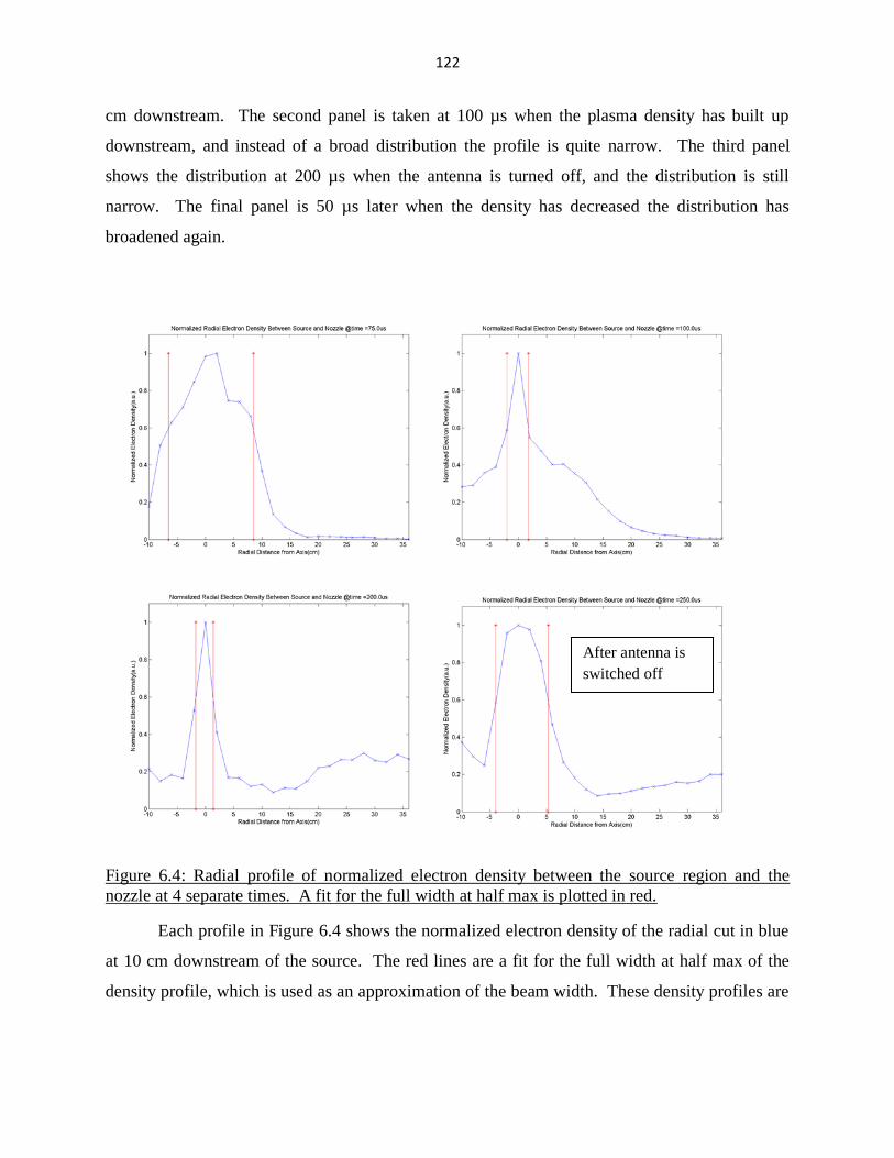
122
cm downstream. The second panel is taken at 100 µs when the plasma density has built up
downstream, and instead of a broad distribution the profile is quite narrow. The third panel
shows the distribution at 200 µs when the antenna is turned off, and the distribution is still
narrow. The final panel is 50 µs later when the density has decreased the distribution has
broadened again.
Figure 6.4: Radial profile of normalized electron density between the source region and the
nozzle at 4 separate times. A fit for the full width at half max is plotted in red.
Each profile in Figure 6.4 shows the normalized electron density of the radial cut in blue
at 10 cm downstream of the source. The red lines are a fit for the full width at half max of the
density profile, which is used as an approximation of the beam width. These density profiles are
After antenna is
switched off
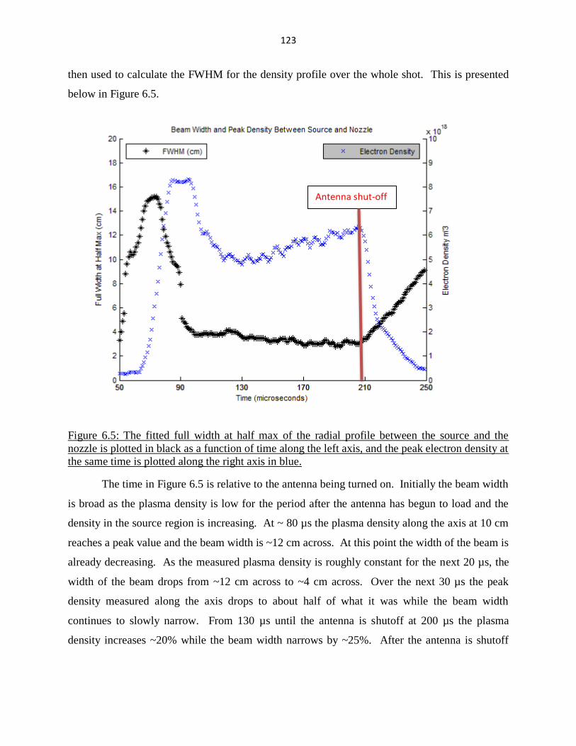
123
then used to calculate the FWHM for the density profile over the whole shot. This is presented
below in Figure 6.5.
Figure 6.5: The fitted full width at half max of the radial profile between the source and the
nozzle is plotted in black as a function of time along the left axis, and the peak electron density at
the same time is plotted along the right axis in blue.
The time in Figure 6.5 is relative to the antenna being turned on. Initially the beam width
is broad as the plasma density is low for the period after the antenna has begun to load and the
density in the source region is increasing. At ~ 80 µs the plasma density along the axis at 10 cm
reaches a peak value and the beam width is ~12 cm across. At this point the width of the beam is
already decreasing. As the measured plasma density is roughly constant for the next 20 µs, the
width of the beam drops from ~12 cm across to ~4 cm across. Over the next 30 µs the peak
density measured along the axis drops to about half of what it was while the beam width
continues to slowly narrow. From 130 µs until the antenna is shutoff at 200 µs the plasma
density increases ~20% while the beam width narrows by ~25%. After the antenna is shutoff
Antenna shut-off

124
and production of plasma in the source region drops off, the density along the axis drops rapidly
while at the same time the width of the beam widens out again.
This narrowing of the beam between the source and the nozzle while the antenna is on
suggests that there is a force acting to push plasma onto the axis while the antenna is on and
plasma is downstream. This is similar to the estimated JxB force towards the axis measured in
Chapter 5. With the increased axial magnetic field between the source and the nozzle, it’s
possible that the region where the azimuthal diamagnetic current crossed with the axial magnetic
field results in a force towards the axis has been extended over a longer region, so that rather
than restricted to a few centimeters near the source exit it is acting over a longer region and
results in a larger acceleration. Normally the electron thermal pressure would be acting to
expand the plasma beam across the magnetic field and would be balanced out by an azimuthal
diamagnetic current causing a JxB force towards the axis and a radial electric force caused by the
motion of the electrons relative to the colder ions, as described by Stenzel et Al [21]. This
narrowing of the beam suggests that the forces acting to confine the beam are dominant over the
electron thermal pressure of the beam between the source and the nozzle.
A second radial profile of the plasma beam was taken downstream of the nozzle at 66 cm
which is more than two magnet radii downstream of the magnetic nozzle. In Figure 6.6 the
normalized radial electron density is plotted for four separate times, again with the full width at
half max plotted in red.

125
Figure 6.6: Radial electron density 66 cm downstream of the source and more than two magnet radii downstream of the nozzle. Normalized density is in blue while the full width at half max is
displayed in red
As in the converging field case, early in time the distribution is broad when the density is
low and narrows down as the plasma density increases, this time reaching a minimum of ~ 10 cm
for the width of the beam. However, unlike the previous case the beam width widens out over
the course of the shot to ~15 cm when the antenna is shutoff and continuing to broaden
afterward. The beam width and peak plasma density at this position downstream of the nozzle
are plotted as a function of time in Figure 6.7.

126
Figure 6.7: The fitted full width at half max of the radial profile downstream of the nozzle is
plotted in black as a function of time along the left axis, and the peak electron density at the same
time is plotted along the right axis in blue. This was measured at 66 cm downstream.
At this position far downstream the density profile builds slowly and peaks relatively late
in time. This is because it’s far enough from the source region that faster plasma particles arrive
much earlier than the slower particles and the density profile is broadened out in time as a result.
As opposed to the profile measured upstream of the nozzle where the density was increasing in
time while the beam width was narrowing, at this point well downstream of the nozzle the beam
is widening over time from ~10 cm to ~15 cm across over the course of the shot, while over the
same time period the density both increases and decreases. This suggests that the confining force
which was keeping the beam width narrow upstream of the nozzle in the converging field case is
not as dominant over the plasma density in the downstream case. However, the beam diameter
widening by a factor of 2-3 is comparatively low considering the background magnetic field
strength has decreased from 150 gauss to < 10 gauss and this measurement was made more than
two dipole radii downstream of the nozzle.

127
After the antenna is shutoff there is a rapid broadening of the beam width as there was in
the upstream case, but the plasma density at this position does not fall as quickly. This is
because at this position downstream the plasma being measured was produced earlier in time and
had to propagate to 66 cm downstream, while in the 10 cm case the plasma did not have to travel
far from the source region to reach the probe. The same dramatic increase in width with a slower
decrease in density suggests that the beam width is correlated with the antenna shutoff as well as
with the plasma pressure at that position.
Section 6.6: Ion velocity downstream of a single magnetic nozzle:
Measurements of the ion velocity at 66 cm downstream of the source region similar to
those presented in Chapter 5 were made downstream of the magnetic nozzle to compare to the
non-nozzle case. The beam width and plasma density measurements presented in Figure 6.7
were taken at the same position downstream as these ion velocity measurements. The ion
velocity distribution of the nozzle and no-nozzle cases are presented for separate times in Figure
6.8, with the non-nozzle velocities plotted in red while the nozzle case is plotted in blue.

128
Figure 6.8: Ion velocity distribution downstream of the magnetic nozzle, 66 cm from the source
region, for four separate times. The peak of the distribution increases over time for the nozzle
case between 150 and 200 µs, but not the case without the nozzle.
In the first panel of Figure 6.8 at 130 µs the beam width is at its narrowest and the plasma
density has begun to build at the position where the velocity is measured. The non-nozzle case
and the nozzle case have the same population of fast ions above 16 km/s, but there are
dramatically more ions at the speed of 14 km/s and slower reaching the detector for the nozzle
case. In the second panel 20 µs later the high velocity population again overlap, but the increase
in slower ions 6-12 km/s in speed is even more dramatic.
In the third panel at 170 µs the two distributions begin to differ in the case of fast ions as
well. At this point in time the beam width of the nozzle case has widened to ~14 cm and so is
broader than earlier in time but the plasma density on axis has reached a peak. In the non-nozzle
case the peak of the distribution has moved to lower velocity and there are fewer fast ions than
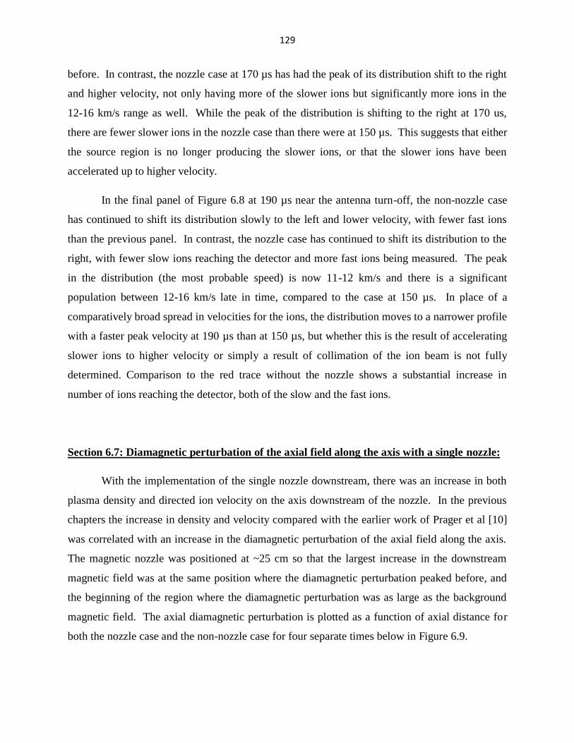
129
before. In contrast, the nozzle case at 170 µs has had the peak of its distribution shift to the right
and higher velocity, not only having more of the slower ions but significantly more ions in the
12-16 km/s range as well. While the peak of the distribution is shifting to the right at 170 us,
there are fewer slower ions in the nozzle case than there were at 150 µs. This suggests that either
the source region is no longer producing the slower ions, or that the slower ions have been
accelerated up to higher velocity.
In the final panel of Figure 6.8 at 190 µs near the antenna turn-off, the non-nozzle case
has continued to shift its distribution slowly to the left and lower velocity, with fewer fast ions
than the previous panel. In contrast, the nozzle case has continued to shift its distribution to the
right, with fewer slow ions reaching the detector and more fast ions being measured. The peak
in the distribution (the most probable speed) is now 11-12 km/s and there is a significant
population between 12-16 km/s late in time, compared to the case at 150 µs. In place of a
comparatively broad spread in velocities for the ions, the distribution moves to a narrower profile
with a faster peak velocity at 190 µs than at 150 µs, but whether this is the result of accelerating
slower ions to higher velocity or simply a result of collimation of the ion beam is not fully
determined. Comparison to the red trace without the nozzle shows a substantial increase in
number of ions reaching the detector, both of the slow and the fast ions.
Section 6.7: Diamagnetic perturbation of the axial field along the axis with a single nozzle:
With the implementation of the single nozzle downstream, there was an increase in both
plasma density and directed ion velocity on the axis downstream of the nozzle. In the previous
chapters the increase in density and velocity compared with the earlier work of Prager et al [10]
was correlated with an increase in the diamagnetic perturbation of the axial field along the axis.
The magnetic nozzle was positioned at ~25 cm so that the largest increase in the downstream
magnetic field was at the same position where the diamagnetic perturbation peaked before, and
the beginning of the region where the diamagnetic perturbation was as large as the background
magnetic field. The axial diamagnetic perturbation is plotted as a function of axial distance for
both the nozzle case and the non-nozzle case for four separate times below in Figure 6.9.
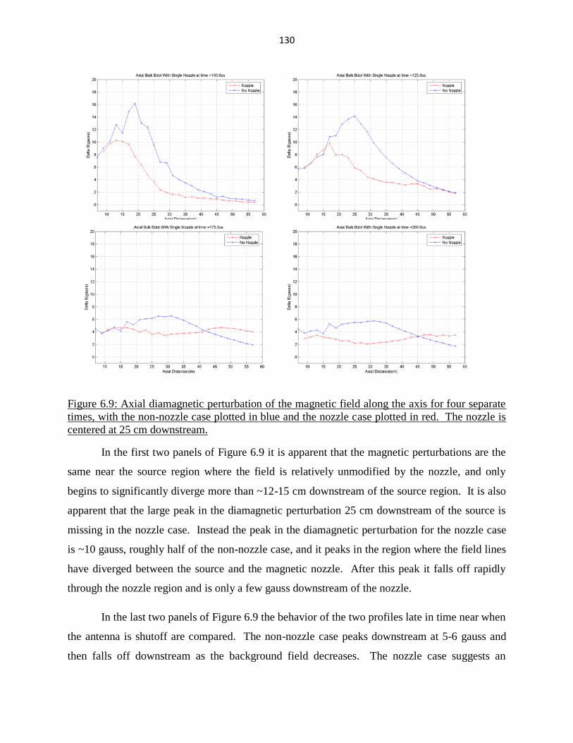
130
Figure 6.9: Axial diamagnetic perturbation of the magnetic field along the axis for four separate
times, with the non-nozzle case plotted in blue and the nozzle case plotted in red. The nozzle is
centered at 25 cm downstream.
In the first two panels of Figure 6.9 it is apparent that the magnetic perturbations are the
same near the source region where the field is relatively unmodified by the nozzle, and only
begins to significantly diverge more than ~12-15 cm downstream of the source region. It is also
apparent that the large peak in the diamagnetic perturbation 25 cm downstream of the source is
missing in the nozzle case. Instead the peak in the diamagnetic perturbation for the nozzle case
is ~10 gauss, roughly half of the non-nozzle case, and it peaks in the region where the field lines
have diverged between the source and the magnetic nozzle. After this peak it falls off rapidly
through the nozzle region and is only a few gauss downstream of the nozzle.
In the last two panels of Figure 6.9 the behavior of the two profiles late in time near when
the antenna is shutoff are compared. The non-nozzle case peaks downstream at 5-6 gauss and
then falls off downstream as the background field decreases. The nozzle case suggests an

131
extended region of ~4 gauss in magnitude near the source region and downstream of the nozzle,
while dropping to ~3 gauss in the region under the nozzle where the magnetic field is high. The
dip in the diamagnetic perturbation is most pronounced in the final panel which shows the
diamagnetic perturbation dropping to ~2 gauss under the nozzle at the time of antenna turn-off.
The position of the nozzle prevented the array of bdot probes used in Chapter 4 from
making a 2D cut of the magnetic field perturbations between the source and the nozzle region,
but based on the axial magnetic perturbation data and the collimation of the beam a rough
estimate of the current density can be made. From the results of the previous chapters, for a peak
diamagnetic perturbation of 10-15 gauss close to the axis this resulted in a diamagnetic current of
~10-20 kAm-2
positioned 2-3 cm from the axis. From the radial Langmuir data it is apparent that
the beam width is ~4 cm for most of the shot, suggesting a similar radial profile is possible.
Since the dominant component of the current was proportional to the radial derivative of the
axial magnetic field perturbation (as described in Chapter 4), the scaled down current estimate
should be proportional to the drop in the diamagnetic perturbation measured. While in the non-
nozzle case the diamagnetic perturbation had a large effect on the total magnetic field, in the case
of the single nozzle the diamagnetic perturbation of the axial field is small compared to the
background magnetic field as plotted in Figure 6.1 as far out as 50 cm downstream.
This means that near the source region early in time, the diamagnetic perturbation being
roughly half what is measured for the non-nozzle case suggests a current density of 5-10 kAm-2
in the region 15-25 cm downstream of the source. In the same position the magnetic field of the
nozzle case is ~100-150 gauss, instead of diamagnetically reduced to near 0. This suggests an
estimated force density of ~150 Nm-3
, which is comparable to that measured near the source
region for the non-nozzle case. What becomes more significant is the region over which the
force is acting, which was a few centimeters long in the non-nozzle case but is tens of
centimeters in the nozzle case. Late in time the diamagnetic perturbation of 3-4 gauss yields a
current estimate of 4-5 kAm-2
over the extended region through the nozzle, while the magnetic
field over that region is still 100-150 gauss even far downstream. This gives an estimate of 50-
75 Nm-3
out as far as 35 centimeters downstream of the source region. So even though this is
only a third of the force acting near the source region in the non-nozzle case, it’s operating over a
length scale more than 15 times longer, yielding a more significant acceleration of ions towards
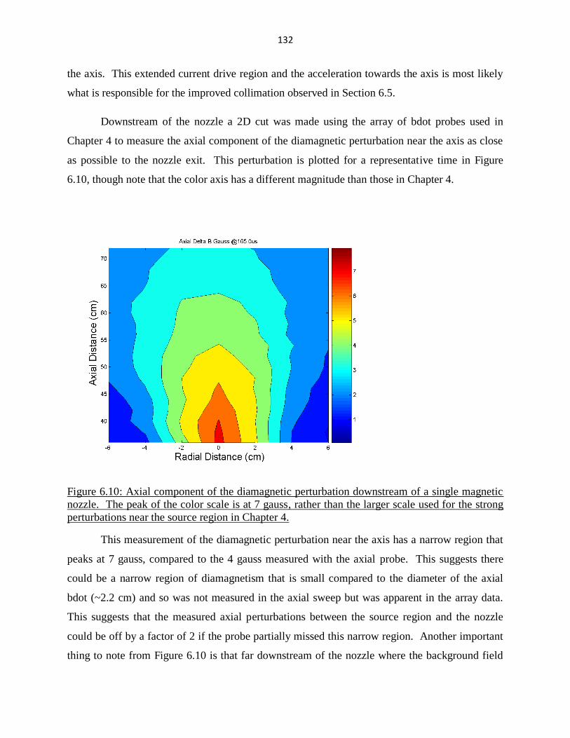
132
the axis. This extended current drive region and the acceleration towards the axis is most likely
what is responsible for the improved collimation observed in Section 6.5.
Downstream of the nozzle a 2D cut was made using the array of bdot probes used in
Chapter 4 to measure the axial component of the diamagnetic perturbation near the axis as close
as possible to the nozzle exit. This perturbation is plotted for a representative time in Figure
6.10, though note that the color axis has a different magnitude than those in Chapter 4.
Figure 6.10: Axial component of the diamagnetic perturbation downstream of a single magnetic
nozzle. The peak of the color scale is at 7 gauss, rather than the larger scale used for the strong
perturbations near the source region in Chapter 4.
This measurement of the diamagnetic perturbation near the axis has a narrow region that
peaks at 7 gauss, compared to the 4 gauss measured with the axial probe. This suggests there
could be a narrow region of diamagnetism that is small compared to the diameter of the axial
bdot (~2.2 cm) and so was not measured in the axial sweep but was apparent in the array data.
This suggests that the measured axial perturbations between the source region and the nozzle
could be off by a factor of 2 if the probe partially missed this narrow region. Another important
thing to note from Figure 6.10 is that far downstream of the nozzle where the background field

133
has dropped to a few gauss, the diamagnetic signal is ~ 3 gauss and so we expect the same sort of
detachment behavior from the diverging nozzle magnetic field as we did from the diverging
source magnetic field. Far enough downstream of the nozzle the diamagnetic effect reduces the
total magnetic field to ~0 and the ions and electrons both can detach from the nozzle magnetic
field.
Since the diamagnetic perturbation of the base field is negligible for the first 50 cm, the
Alfven speed is going to be determined mostly by the strength of the base magnetic field and the
plasma density. The Alfven speed on axis is plotted below in Figure 6.11, with the Alfven speed
in km/s in blue, the fast ion population measured 66 cm downstream in red, and the most
probable speed late in time measured 66cm downstream in green.
Figure 6.11: Alfven speed downstream along the axis with a single magnetic nozzle. The blue
points represent the Alfven speed at that position, while the red line is the measurement of the
fast ion population at 66 cm downstream and the green line is the most probable speed of the
ions measured at 66 cm downstream.
0
5
10
15
20
25
30
8 18 28 38 48 58
Alfven Speed (km/s) with Single Nozzle Downstream
Axial Distance (cm)
Alfven Speed km/s Most Probable Speed
Fast Ion Population

134
The increase in the magnetic field downstream has increased the Alfven speed
downstream dramatically. The increase is high enough that it is likely only that the fastest
component of the ion velocity distribution becomes super-alfvenic upstream of the magnetic
nozzle. It is likely that most of the ions don’t become super-alfvenic until the diverging section
downstream of the nozzle. Since the large diamagnetic perturbation observed in Chapter 4
weakened the magnetic field near the axis the ions were predicted in Chapter 5 to have become
super-alfvenic roughly 20-25 cm downstream of the source, while now that is expected to
happen roughly 1-2 magnet radii downstream of the magnetic nozzle.
Section 6.8: Ion energies upstream and downstream of a second magnetic nozzle:
A second magnetic nozzle was added downstream of the first nozzle to further increase
the magnetic field downstream. This second nozzle had the advantage of being twice the
diameter of the first nozzle, ~50 cm, and was capable of generating magnetic fields of hundreds
of gauss. This allowed the second nozzle to make the magnetic field along the axis downstream
of the source on the same magnitude as the source region, but with a larger radii so that the field
fell off at a slower rate. The axial component of the magnetic field for this new configuration of
two nozzles is presented in Figure 6.12.

135
Figure 6.12: A second nozzle is added downstream of the first centered ~78 cm downstream of
the source region. The second nozzle has a diameter twice that of the first nozzle, which itself is
twice that of the base magnetic field coils.
The second nozzle was positioned far enough downstream of the first nozzle so that the
RFA positioned at 66 cm which took the ion velocity measurements presented above was now
measuring the ion energies in the converging region of the nozzle, while a second RFA
positioned 144 cm downstream could be used to measure the ion energies more than 2 magnet
radii downstream of the second nozzle exit. A side-view of the magnetic field geometry of these
two nozzle coils together with the Earth’s magnetic field are presented in Figure 6.13.

136
Figure 6.13: Magnetic field of the two nozzle configuration with the Earth’s magnetic field.
Magnetic field does not drop below 100 gauss until more than 1 m downstream of the source
region.
This new configuration has a larger magnetic pressure than the previous nozzle
configuration downstream, and so it’s expected that the bulk of the plasma stays near the axis
from the source region through the second nozzle. Also similarly to the previous case with one
nozzle, radial profiles of the plasma density upstream of these nozzles show a well collimated
plasma beam near the axis, that has the beam width decrease over the course of the shot.
One concern with a large converging magnetic field was whether part of the plasma
population would be slowed down or turned back by the nozzle. In the converging nozzle data
of Inutake et al, there was a decrease in the directed ion energy as a result of the converging
magnetic field. To determine if this was occurring with the nozzles of HPH, ion energies were
measured both upstream and downstream of the second magnetic nozzle. The integrated current
to the RFA upstream of the nozzle as a function of ion energy is presented in Figure 6.14.

137
Figure 6.14: RFA Collector Current as a function of retarding voltage integrated over the entire
plasma shot, upstream of the second magnetic nozzle. The blue curve represents the ion
population with the second nozzle turned off, while the red curve is with the second nozzle on.
The RFA collects ions that have a directed ion energy greater than or equal to the
retarding potential on the discriminator grid. By integrating the current received at the RFA over
the course of the whole plasma shot and plotting it as a function of discriminator voltage, it can
be determined if there is a significant portion of the ion energy population that is being slowed or
turned back upstream of the second magnetic nozzle. For the higher energy ion components
above 40 eV, the non-nozzle case and the nozzle case match up well and it does not appear as if
the higher energy ions are slowing down. It’s possible that the population of ions with energies
20-40 eV are being partly slowed down by the converging magnetic field, as there are fewer of
them on the axis than in the non-nozzle case. There is also roughly twice as many low energy
ions on axis in the nozzle case as there are in the non-nozzle case. The same measurement was
also made 145 cm downstream of the source region on the other side of the second magnetic
138
nozzle and more than 2 magnet radii downstream of it. These results are presented in Figure
6.15.
Figure 6.15: RFA Collector Current as a function of retarding voltage, integrated over the entire
plasma shot, downstream of the second magnetic nozzle. The blue curve represents the ion
population with the second nozzle turned off, while the red curve is with the second nozzle on.
Comparing the two populations in Figure 6.15 downstream of the second nozzle, it does
not appear as though there is a significant population of ions that is prevented from passing
through the second nozzle downstream. At each energy level there are as many or more ions
downstream of the nozzle with it than with it off, with the difference being roughly a factor of 2
for the higher energy ions and a factor of 5 for the lower energy population. So even though the
magnetic field inside the second nozzle is on the same order as the base magnetic field in the
source region, it is unlikely that there is a significant population of ions that are trapped by the
second nozzle and not able to get through. It is more likely that the case of HPH is closer to the

139
model described by Arefiev et Al [28] of cold ions that are unmagnetized being accelerated
through the nozzle instead of slowing to conserve magnetic moment.
Modifying the magnetic field downstream of the source region with magnetic nozzles had
a substantial impact on the collimation of the plasma beam and the flow velocity of the plasma
downstream. In the next chapter results from modifying the downstream magnetic field with
both nozzles and a second helicon wave source to improve the collimation and ion velocity
further are presented.

140
Chapter 7: Increased Helicon Wave Power with the Addition of a Second Antenna Downstream
Section 7.1: Wave Frequency, Input Power, and Effect on Performance
In the previous chapter, modifications made to the magnetic field downstream of the
helicon source by magnetic nozzles resulted in an increase in downstream directed ion velocities
and axial collimation of the plasma plume. This magnetic field configuration caused the
diamagnetic perturbation along the axis to be reduced in magnitude compared to the
measurements presented in Chapter 4 but was observed over a longer axial distance. One
possible explanation for this was that the increase in the background magnetic field prevented the
diamagnetic perturbation from effectively reducing the magnetic field to ~0 (as was measured in
Chapter 4) and this allowed the wave driven by the antenna to propagate further along the axis.
By propagating further downstream this extended the region over which a diamagnetic current
was driven in the plasma by interaction with the helicon wave and increased the region of JxB
acceleration of the plasma particles, resulting in a faster ion population downstream on axis with
the nozzle on. As discussed previously in chapters 4 and 5 there is a correlation between the
diamagnetic perturbation observed in the plasma and the magnitude of the helicon wave
magnetic field (measured in gauss) measured downstream, with the wave magnetic field being
roughly equal to the total background field in the data presented in chapter 4. The diamagnetic
perturbation had already been correlated in time and space with the antenna being on, and the
next step in my research was to correlate the diamagnetic perturbation with the frequency and
power of the wave magnetic field so that we have a mechanism in hand in order to further
enhance the effect.
In Chapter 5 I suggested the possibility that the diamagnetic current that was measured
downstream was being directly driven by the wave magnetic field as it rotated some fraction of
the electron population around the axis at the antenna frequency before they were stopped by
collisions with other plasma particles. The collision rate for electrons downstream was roughly 3
times that of the antenna frequency, so that if only about a third of the particles were contributing

141
to the current that would roughly match the measured current density. If this was the case, then
increasing or decreasing the frequency of the helicon wave being driven downstream would
increase or decrease the current density in the plasma directly. The difficulty mentioned in
chapter 5 with testing this was that changing the frequency of the wave being driven downstream
required changing the frequency of the source antenna, and that would have other consequences
on the plasma output of the source region.
In the standard model of helicon wave propagation developed by F.F. Chen and others
[12], the dispersion relationship of the helicon wave propagating along a uniform axial magnetic
field with a uniform plasma density and with an insulating boundary is given by:
83.3
0
0
0 aeu
kn
B
z
, 7.1
where B0 is the background magnetic field strength, n0 is the background plasma density, ω is the
angular frequency of the wave, e and u0 are constants, and ‘a’ is the radius of the boundary layer
and antenna wrapped around it. While these conditions don’t hold downstream of the source
region of the HPH, they are similar to the conditions inside the source region of HPH where the
neutrals are ionized into plasma and the background magnetic field is more uniform. Previous
work with the HPH by Prager et Al [11] established that axial wavelength of the plasma wave
was determined by the physical length of the antenna and the angular frequency was determined
by the frequency at which the oscillating current in the source antenna was driven by the power
supply, similar to other helicon experiments. Re-writing equation 7.1 to reflect this, we have the
relationship:
0
0 83.3
euaf
Bne
, 7.2
where ne is the electron density, f is the frequency of the source antenna, and λ is the wavelength
of the source antenna (the physical antenna is half-wavelength as described in chapter 2).
Equation 7.2 suggests that the stronger the background magnetic field in the source region the
higher the resultant electron density will be, and this was confirmed by observations made by
Ziemba [9] and Prager [2] up until the limits of the antenna power supply were reached. This is
because unless there is enough power coupling from the source antenna to the plasma to sustain

142
the discharge against losses due to recombination and flow of the plasma out of the source region
[2] the electron density cannot be increased further. This established the upper limit of the
performance of the HPH plasma source to be mostly determined by the limitation of the rate at
which power can be deposited by the source antenna into the plasma [9].
The frequency of the helicon wave in eq. 7.2 is inversely related to the background
electron density, suggesting that if we increase the antenna frequency we would need to increase
the background magnetic field B0 proportionally to keep the same background density.
However, increasing the background magnetic field will affect other areas of the plasma
production, such as determining the plasma beta and the Alfven speed. Increasing the
background magnetic field will also alter the relationship between the magnitude of the wave
magnetic field and background magnetic field discussed in chapters 4 and 5, possibly altering the
behavior of the wave downstream. If the background magnetic field is instead kept the same,
then the expectation would be for the density in the source region to decrease. This will decrease
the plasma beta as well, and there will be fewer electrons in the source region and downstream to
flow in diamagnetic currents.
Because of these consequences to the plasma source production with the change in the
source antenna frequency (as well as wave amplitude as seen in the following section), it is
difficult to determine the relationship between the measured diamagnetic currents downstream of
the source and the wave frequency by just modifying the frequency of the source antenna.
Instead, for the bulk of this chapter a second helicon antenna is introduced downstream of the
source antenna that can be modified independently of the source antenna. This allows for the
modification of the antenna frequency of the second antenna without significantly affecting the
plasma production in the source region. The introduction of the second antenna is shown to
produce an increase in the performance of HPH and will be detailed in the following sections.
Section 7.2: Results from Increasing Frequency, Decreasing Antenna Current of the Source
Antenna
Prior to the introduction of the second downstream antenna, the frequency of the source
antenna was changed to measure some of the effects on the measured diamagnetic perturbation
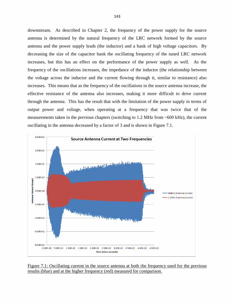
143
downstream. As described in Chapter 2, the frequency of the power supply for the source
antenna is determined by the natural frequency of the LRC network formed by the source
antenna and the power supply leads (the inductor) and a bank of high voltage capacitors. By
decreasing the size of the capacitor bank the oscillating frequency of the tuned LRC network
increases, but this has an effect on the performance of the power supply as well. As the
frequency of the oscillations increases, the impedance of the inductor (the relationship between
the voltage across the inductor and the current flowing through it, similar to resistance) also
increases. This means that as the frequency of the oscillations in the source antenna increase, the
effective resistance of the antenna also increases, making it more difficult to drive current
through the antenna. This has the result that with the limitation of the power supply in terms of
output power and voltage, when operating at a frequency that was twice that of the
measurements taken in the previous chapters (switching to 1.2 MHz from ~600 kHz), the current
oscillating in the antenna decreased by a factor of 3 and is shown in Figure 7.1.
Figure 7.1: Oscillating current in the source antenna at both the frequency used for the previous
results (blue) and at the higher frequency (red) measured for comparison.
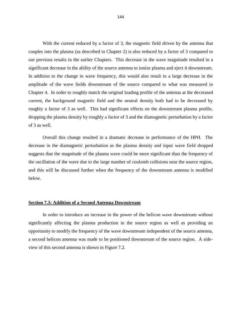
144
With the current reduced by a factor of 3, the magnetic field driven by the antenna that
couples into the plasma (as described in Chapter 2) is also reduced by a factor of 3 compared to
our previous results in the earlier Chapters. This decrease in the wave magnitude resulted in a
significant decrease in the ability of the source antenna to ionize plasma and eject it downstream.
In addition to the change in wave frequency, this would also result in a large decrease in the
amplitude of the wave fields downstream of the source compared to what was measured in
Chapter 4. In order to roughly match the original loading profile of the antenna at the decreased
current, the background magnetic field and the neutral density both had to be decreased by
roughly a factor of 3 as well. This had significant effects on the downstream plasma profile,
dropping the plasma density by roughly a factor of 3 and the diamagnetic perturbation by a factor
of 3 as well.
Overall this change resulted in a dramatic decrease in performance of the HPH. The
decrease in the diamagnetic perturbation as the plasma density and input wave field dropped
suggests that the magnitude of the plasma wave could be more significant than the frequency of
the oscillation of the wave due to the large number of coulomb collisions near the source region,
and this will be discussed further when the frequency of the downstream antenna is modified
below.
Section 7.3: Addition of a Second Antenna Downstream
In order to introduce an increase in the power of the helicon wave downstream without
significantly affecting the plasma production in the source region as well as providing an
opportunity to modify the frequency of the wave downstream independent of the source antenna,
a second helicon antenna was made to be positioned downstream of the source region. A side-
view of this second antenna is shown in Figure 7.2.
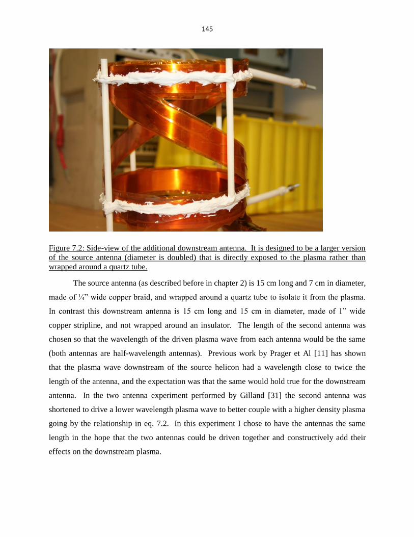
145
Figure 7.2: Side-view of the additional downstream antenna. It is designed to be a larger version
of the source antenna (diameter is doubled) that is directly exposed to the plasma rather than
wrapped around a quartz tube.
The source antenna (as described before in chapter 2) is 15 cm long and 7 cm in diameter,
made of ¼” wide copper braid, and wrapped around a quartz tube to isolate it from the plasma.
In contrast this downstream antenna is 15 cm long and 15 cm in diameter, made of 1” wide
copper stripline, and not wrapped around an insulator. The length of the second antenna was
chosen so that the wavelength of the driven plasma wave from each antenna would be the same
(both antennas are half-wavelength antennas). Previous work by Prager et Al [11] has shown
that the plasma wave downstream of the source helicon had a wavelength close to twice the
length of the antenna, and the expectation was that the same would hold true for the downstream
antenna. In the two antenna experiment performed by Gilland [31] the second antenna was
shortened to drive a lower wavelength plasma wave to better couple with a higher density plasma
going by the relationship in eq. 7.2. In this experiment I chose to have the antennas the same
length in the hope that the two antennas could be driven together and constructively add their
effects on the downstream plasma.

146
In order to help prevent the two antennas from destructively interfering with each other,
the second antenna was placed downstream with a half-wavelength spacing between the two
antennas. This required a modification to the background magnetic field from the previous
nozzle work presented in Chapter 6. This new magnetic field geometry is shown Figure 7.3:
Figure 7.3: Side-view of the magnetic field geometry with the addition of the downstream
antenna. The magnetic field diverges upon leaving the source region but still passes through the
larger diameter downstream antenna before significantly diverging or connecting with the
Earth’s magnetic field more than 60 cm downstream.
In this diagram the source antenna is positioned from -15 cm to 0 cm along the axis,
while the downstream antenna is positioned from 15 cm to 30 cm downstream along the axis.
The magnetic field lines that pass through the source antenna (within ~3.5 cm of the axis)
expand out slightly when passing through the region where the downstream antenna is
positioned, but do not approach the physical boundaries of the second antenna, which are ~7.5
cm from the axis. Radial electron density profiles taken 15 cm downstream of the source region
where the electrons are still well-magnetized (as discussed in Chapter 4) indicate that the bulk of
the plasma is near the axis and has not expanded radially across the magnetic field a significant

147
distance. This means that the majority of the plasma particles that exit the source region will still
be near the axis when they enter the second antenna and will not have expanded far enough
radially to pass outside the second antenna.
As the magnetic field from the source region and the downstream nozzles expand, the
axial component of the magnetic field decreases. For the region where the second downstream
antenna is operated, the magnetic field along the axis has decreased by roughly a factor of 2 from
what it was in the source region, going from varying between 400-480 gauss in the source region
to 200-280 gauss in the downstream antenna. In both cases the magnetic field decreases along
the length of the antenna instead of being a uniform solenoid field. It was anticipated that the
diverging and decreasing magnetic field would improve the acceleration of the plasma out of the
source region and out of the downstream antenna region. The axial profile of this magnetic field
is shown in figure 7.4:
Figure 7.4: Profile of the axial component of the base magnetic field along the axis in the new
configuration to support the downstream antenna. The magnetic field peaks near the rear of the
source antenna and is between 400-480 gauss in the source region. The magnetic field decreases
in the downstream antenna region to 200-280 gauss before falling off like a dipole field beyond
the last set of magnetic coils.

148
The decrease in base magnetic field is necessary because the downstream antenna with its
larger diameter is expected to drive a weaker magnetic field along the axis than the source
antenna. Even if the same power could be coupled through both antennas, the increased volume
of the second antenna suggests that the energy density of the driven magnetic field should be
lower in the downstream antenna than the source antenna. In Chapter 4 it was found that
downstream of the source with no nozzles present the diamagnetic perturbation was strongest
when the wave magnetic field of the source along the axis was comparable in magnitude to the
base magnetic field. So by having the magnetic field decrease by roughly a factor of 2 at the
same time the distance from the antenna coils to the axis increased by a factor of 2, there is a
better chance at keeping the ratio of wave magnetic field to base magnetic field in the non-linear
regime.
Section 7.4: Initial Effect of the Downstream Antenna on Ion Energies
Initial tests of the downstream antenna were performed with the second antenna operating
at the same frequency for the full 400 microseconds that the source antenna was on, being turned
on at the same time as the source antenna. To compare the effect of the second antenna being
active on the plasma, the argon ion energies were measured well downstream of the exit of the
second antenna. It became apparent quickly that while the HPH source produced a nearly
identical plasma population each shot, with the downstream antenna on the plasma population
was not being reproduced in a repeatable matter. In Figure 7.5, the ion current measured by the
downstream RFA is presented at four discriminator voltages, firing the system for 10 shots in
succession with the second antenna on (red) compared to firing for 5 shots in a row with the
antenna off (blue).
149
Figure 7.5: Shot to shot variability of ion current to the collector at four discriminator voltages
prior to adjusting the downstream antenna. The downstream antenna is shown to be capable of
both increasing and decreasing the population of energetic ions downstream, though it more
frequently increases them by some amount.
For the first set of data points with 0V on the discriminator grid (where all the ions reach
the collector), the total amount of argon ions reaching the downstream RFA on axis is roughly
the same for many of the shots. It is expected that the total ion population is not significantly
increased because the second antenna is not expected to ionize a significant amount of neutral
argon. The neutral argon atoms are not expected to move beyond the source region while the
downstream antenna is on because the sound speed of the neutral argon is slow compared to the
short operation time of the experiment and the distance to the second antenna from the gas puff.
Instead, this increase of ions reaching the detector comes from a decrease in ions drifting away
from the axis missing the RFA on axis.

150
The next significant set of data for the ions with energies greater than 30 eV show that
with the second antenna on there a significant increase in the number of ions with energies above
30 eV for the bulk of the shots taken. But at the same time, there were also examples of roughly
the same amount of ions at the energy, and one significant case where there are dramatically
fewer ions with energies >30 eV, which shifts both up and down of roughly 33%. This
characteristic is seen again for the shots taken measuring the ion population with energies >50
eV. Depending on the shot taken, the second antenna is either enhancing the number fast ions,
diminishing the number of fast ions, or doing nothing. For the case of argon ions with energies
>70 eV, there was no example of the second antenna decreasing the population, but several
examples of it nearly doubling the amount of energetic ions measured at the downstream RFA.
To help determine what the mechanism was behind whether the second antenna was
accelerating ions, decelerating ions, or doing nothing, the loading profile of the downstream
antenna was examined for 3 of the shots taken with the ion currents at different extremes. Figure
7.6 represents the loading profile where there was maximum acceleration of the ions, Figure 7.7
represents the case where there was maximum deceleration of the ions, and Figure 7.8 is the case
where there was no significant difference between when the antenna was on or off.
Figure 7.6: Current profile of the downstream antenna that resulted in the maximum current of
energetic ions to the downstream RFA. This represents the case where the second antenna is
providing a maximum acceleration to the ions.
50V Max
-4.00E+02
-3.00E+02
-2.00E+02
-1.00E+02
0.00E+00
1.00E+02
2.00E+02
3.00E+02
4.00E+02
0.00E+00 1.00E-04 2.00E-04 3.00E-04 4.00E-04 5.00E-04 6.00E-04
Time (microseconds)
DS
An
ten
na
Cu
rre
nt(
A)

151
Significant properties of this loading profile include: there is a dramatic change in the
current in the antenna at roughly 80 microseconds in when the bulk of the plasma from the
source antenna reaches the second antenna. For roughly 150 microseconds the loading profile is
flat, but this is followed by several events when the antenna seems to change its loading profile
repeatedly for the rest of the 400 microseconds.
Figure 7.7: Current profile of the downstream antenna that resulted in minimum current of
energetic ions to the downstream RFA. This represents the case where the second antenna is
providing a significant deceleration to the ions and the plasma outflow is slower than with the
second antenna turned off.
In this profile the plasma appears to arrive at the same time, but instead of a relatively
stable period there is even more erratic behavior in the loading profile. It isn’t immediately clear
what aspect of the profile results in a deceleration of the ions rather than acceleration.
50V Min
-4.00E+02
-3.00E+02
-2.00E+02
-1.00E+02
0.00E+00
1.00E+02
2.00E+02
3.00E+02
4.00E+02
0.00E+00 1.00E-04 2.00E-04 3.00E-04 4.00E-04 5.00E-04 6.00E-04
Time (microseconds)
DS
An
ten
na
Cu
rre
nt
(A)

152
Figure 7.8: Current profile of the downstream antenna that resulted in roughly the same number
of energetic ions reaching the RFA as when the second antenna is turned off. This represents the
case when the second antenna is oscillating but has a net effect of zero.
In this last profile, the loading profile appears to be very similar to the profile in 7.6
which results in the maximum acceleration, with a period of loading after the plasma arrives
followed by several events where the antenna appears to unload and load again repeatedly. The
main difference between the two is that the profile in 7.8 does not have as long as a stable period
of loading as occurred in 7.6.
By comparing these loading profiles, it wouldn’t be feasible to identify the real
performance of the downstream antenna unless the antenna was configured to repeatedly
generate the same accelerated population shot to shot without this large variation in effect. This
involved both identifying why the loading profile of the second antenna varied so much and to
come up with a method to limit it.
Section 7.5: Synchronizing the Downstream Antenna
In each of the loading profiles shown above (7.6-7.8) there is a dramatic change in the
antenna current profile roughly 80 microseconds after the source antenna is turned on and the
50V effectively off
-4.00E+02
-3.00E+02
-2.00E+02
-1.00E+02
0.00E+00
1.00E+02
2.00E+02
3.00E+02
4.00E+02
0.00E+00 1.00E-04 2.00E-04 3.00E-04 4.00E-04 5.00E-04 6.00E-04
Time (microseconds)
DS
An
ten
na C
urr
en
t (A
)

153
bulk of the plasma from the source antenna arrives inside the downstream antenna. In these first
80 microseconds when there is plasma present under one antenna but not the second, my
expectation is that the two antennas (even though they are being driven at the same time at the
same frequency) are not in phase, and there is an abrupt shift when the plasma arrives under the
second antenna along with the plasma wave from the source antenna. Later in the shot after the
bulk of the plasma pulse has passed through both antennas and moved downstream, there is a
non-repeatable series of loading/unloading events like seen in the previous loading profiles.
Because of these two properties, the second antenna is not turned on until both plasma
and the driven plasma wave from the source antenna are present under the antenna, roughly
85.76 microseconds after the source antenna is turned on. Similarly, rather than leave the second
antenna on and have the non-repeatable loading pattern the antenna is turned off ~160
microseconds after the second antenna was turned on when the plasma population under the
second antenna has fallen off in density. Both of these values were arrived at through repeated
firing of the experiment and adjusting the settings of the two antennas to arrive at a repeatable
configuration of the second antenna that also resulted in an accelerated ion population similar to
the maximum seen in Figure 7.5. The loading profile of this configuration is shown below in
Figure 7.9.

154
Figure 7.9: Loading profile of the downstream antenna that is repeatable shot to shot and results
in a significant increase in the downstream ion energies. Note that the second antenna current is
lower than the source antenna, and is only active for a fraction of the time.
The current in the downstream antenna does not ring up to as high of a current as seen
when there is no plasma present under the second antenna, but the maximum current measured
(300-400 Amps peak to peak) is higher than what was observed during the relatively stable
loading region in Figure 7.6 by 50-100%. There is some variation in the loading profile as the
bulk of the plasma arrives and leaves similar to that seen in the source antenna when the neutrals
are ionized and then ejected from the source region. For comparison, the loading profile of the
source antenna for the same configuration is show below in Figure 7.10:

155
Figure 7.10: Loading profile of the source antenna. This matches closely with the loading profile
measured with the data taken in the previous chapters and can be directly compared.
This loading profile matches closely with what was previously measured for the source
region in the previous chapters when the source antenna was on for 400 microseconds. There is
significantly more current oscillating in the source antenna compared to the downstream antenna,
and the source is continuing to ionize neutrals into plasma for 150 microseconds after
downstream antenna is turned off. Unfortunately the downstream antenna was not able to
reliably load in that period to keep accelerating the ion population made late in time. This
configuration of the two antennas was repeatable shot to shot comparable to the previous data
presented in the earlier chapters with just the source antenna.
Section 7.6: Increased Ion Velocities with the Downstream Antenna
With this new repeatable configuration a series of shots was taken and the ion energy
distribution function of the ions downstream of both antennas was measured similar to the data
presented in chapters 5 and 6. The current profile at the RFA on axis at a time of peak signal is
shown below in Figure 7.11:
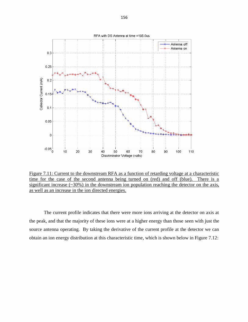
156
Figure 7.11: Current to the downstream RFA as a function of retarding voltage at a characteristic
time for the case of the second antenna being turned on (red) and off (blue). There is a
significant increase (~30%) in the downstream ion population reaching the detector on the axis,
as well as an increase in the ion directed energies.
The current profile indicates that there were more ions arriving at the detector on axis at
the peak, and that the majority of these ions were at a higher energy than those seen with just the
source antenna operating. By taking the derivative of the current profile at the detector we can
obtain an ion energy distribution at this characteristic time, which is shown below in Figure 7.12:
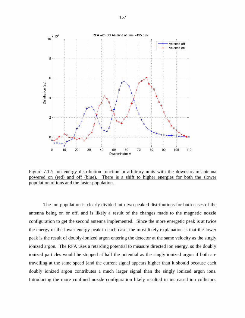
157
Figure 7.12: Ion energy distribution function in arbitrary units with the downstream antenna
powered on (red) and off (blue). There is a shift to higher energies for both the slower
population of ions and the faster population.
The ion population is clearly divided into two-peaked distributions for both cases of the
antenna being on or off, and is likely a result of the changes made to the magnetic nozzle
configuration to get the second antenna implemented. Since the more energetic peak is at twice
the energy of the lower energy peak in each case, the most likely explanation is that the lower
peak is the result of doubly-ionized argon entering the detector at the same velocity as the singly
ionized argon. The RFA uses a retarding potential to measure directed ion energy, so the doubly
ionized particles would be stopped at half the potential as the singly ionized argon if both are
travelling at the same speed (and the current signal appears higher than it should because each
doubly ionized argon contributes a much larger signal than the singly ionized argon ions.
Introducing the more confined nozzle configuration likely resulted in increased ion collisions

158
near the axis that doubly ionized a small fraction of the total ion population after the ions had
already been accelerated, resulting in a two peaked distribution whether the second antenna is on
or off.
The case of the second antenna being on (red) has the singly ionized population shifted
up by ~ 20-25 eV. Additionally, the width of the population is broader in the case of the second
antenna being on with an extended tail with some ions having >100 eV. Making the same
assumptions made earlier with respect to the RFA (no significant plasma potential acceleration,
singly ionized argon, etc), the ion energy distribution function can be converted into an ion
velocity distribution function for the same time in Figure 7.13:
7.13: Ion velocity distribution function for the case of the downstream antenna powered on (red)
and off (blue). The ion population is 2-5 km/s faster with the second antenna on.
It’s clear in this result that the ion population has been accelerated by the downstream
antenna by several km/s in the downstream direction. The bulk of the plasma population is

159
travelling 18-22 km/s which is a significant increase over the velocities previously measured
with HPH using only one antenna. A more detailed description of the ion energies as a function
of time will be presented later in this chapter in section 7.11.
Section 7.7: Improved Collimation of the Beam with the Downstream Antenna
In addition to the increased ion velocities measured downstream of the second antenna,
there was an improvement in the collimation of the plasma plume downstream of the second
antenna when it was on compared to just the single antenna. The blue light emission from the
ionized argon in the downstream antenna is shown below in Figure 7.14:
Figure 7.14: Side view of the second antenna downstream while firing. This is a 400
microsecond exposure that captures the entire experimental run, and it can be clearly seen that
there is a blue column of ionized argon along the axis of the second antenna. The occasional
bright spot on the antenna suggests there could be some direct interaction between the plasma
and the copper of the antenna.

160
As described earlier in section 7.3, the bulk of the plasma is expected to be near the axis
while inside the second antenna due to the magnetic field of the nozzles and this is visually
apparent from the intense light emission in Figure 7.14, with only a diffuse glow off the axis and
near the copper surface of the antenna. Beyond the exit of the second antenna and the magnetic
nozzles, a radial profile of the electron density was made 109 cm downstream of the source
where the ion energies were measured with the RFA to show the collimation of the beam more
than one nozzle diameter downstream of the nozzle exit. This radial profile is shown below in
Figure 7.15 at the characteristic time shown above in the ion RFA results:
Figure 7.15: Radial profile of the electron density taken with a symmetric double Langmuir
probe for the case of the downstream antenna being on (black), the downstream antenna being
off but with the nozzles power on (blue), and without either the downstream antenna or the
nozzles (red). There is an increase in density along the axis of ~30%; similar to what was
measured with the downstream RFA at approximately the same axial location.

161
The trace in red shows the radial profile of the plasma with only the source antenna active
and none of the magnetic nozzles similar to the plasma produced in the data presented in chapter
4. The blue trace is the plasma profile with only the source antenna on, but with the magnetic
nozzles on in the configuration to support the second antenna. Lastly, the black trace is the case
with both antennas and the nozzles on, showing that there is an increase in the plasma density
along the axis (and decrease off axis) with the second antenna being on as high as 30%. This
corroborates the increase in current measured by the collector of the RFA. Enhancing the
directed ion energies and collimation of the ion population is a primary goal of this work, and the
next step is to see if the magnetic diagnostics similar to those used in previous chapters can help
explain the improvement seen with the second antenna downstream.
Section 7.8: Diamagnetic Perturbation with the Downstream Antenna
Using an axial magnetic field b-dot probe like the one used in chapter 4 to measure the
diamagnetic perturbation to the base magnetic field, the axial diamagnetic perturbation was
measured both between the two antennas and downstream of the second antenna. The mounting
for the probe was too large to fit inside the second antenna, so there is a gap in the data for nearly
20 cm when the probe had to be moved around the downstream antenna. In this region the
magnetic field supplied by the nozzle is large compared to these perturbations (as shown in
Figure 7.4), and even though the axes in the graphs are positive, this is a diamagnetic
perturbation of the background magnetic field. The diamagnetic perturbation of the axial
component of the background field is shown for both the case of the source antenna only (blue)
and both antennas firing (red) is plotted for characteristic times during the build-up of the shot
below in Figure 7.16:
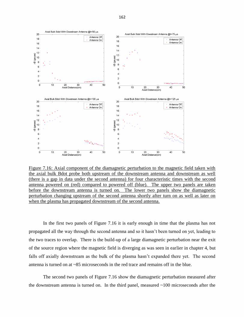
162
Figure 7.16: Axial component of the diamagnetic perturbation to the magnetic field taken with
the axial bulk Bdot probe both upstream of the downstream antenna and downstream as well
(there is a gap in data under the second antenna) for four characteristic times with the second
antenna powered on (red) compared to powered off (blue). The upper two panels are taken
before the downstream antenna is turned on. The lower two panels show the diamagnetic
perturbation changing upstream of the second antenna shortly after turn on as well as later on
when the plasma has propagated downstream of the second antenna.
In the first two panels of Figure 7.16 it is early enough in time that the plasma has not
propagated all the way through the second antenna and so it hasn’t been turned on yet, leading to
the two traces to overlap. There is the build-up of a large diamagnetic perturbation near the exit
of the source region where the magnetic field is diverging as was seen in earlier in chapter 4, but
falls off axially downstream as the bulk of the plasma hasn’t expanded there yet. The second
antenna is turned on at ~85 microseconds in the red trace and remains off in the blue.
The second two panels of Figure 7.16 show the diamagnetic perturbation measured after
the downstream antenna is turned on. In the third panel, measured ~100 microseconds after the

163
source antenna was turned on and roughly ~15 microseconds after the second antenna was turned
on, the diamagnetic perturbation between the two antennas is increased by 2 gauss with the
second antenna on, a change of ~15-20%. At the same time, downstream of the second antenna
the bulk of the plasma hasn’t expanded far enough and the two traces are still low and roughly
equal. In the fourth panel of Figure 7.16 measured at 125 microseconds the diamagnetic
perturbation between the two antennas remains high for the case of the second antenna on, but
has decreased for the case of the downstream antenna off, making the enhancement an
improvement of ~40% in the region between the two antennas. There is also a difference in the
behavior of the diamagnetic perturbation far downstream of the second antenna, with an increase
of ~2 gauss again, this is an increase of ~50% over the case of just the source antenna acting by
itself in the region well downstream of the antennas.
To look at the behavior of the perturbation later in time and near the turn-off of the
antennas, the diamagnetic perturbation for the two cases is plotted for four additional times
below in Figure 7.17:

164
Figure 7.17: Axial component of the diamagnetic perturbation to the magnetic field taken with
the axial bulk Bdot probe both upstream of the downstream antenna and downstream as well
(there is a gap in data under the second antenna) for four characteristic times showing the
evolution of the profile with time and after the second antenna is shut off. The upper two panels
are taken before the downstream antenna is turned off and show the maximum downstream
diamagnetic perturbation as well as the decrease later in time after the bulk of the plasma has
moved through the second antenna. The lower two panels show the diamagnetic perturbation
after the downstream antenna is shut off but while the source antenna is still active.
In the first panel of Figure 7.17, 150 microseconds into the shot the diamagnetic
perturbation has begun to decrease in both traces, as the bulk of the plasma moves out from the
region of the two antennas and downstream of the thruster. In the gap between the antennas
there is still a ~2-4 gauss increase while downstream of the second antenna it has fallen to a
difference of ~1-2 gauss, or an increase of ~25-40% over the case with only the source antenna
on. In the second panel of Figure 7.17 at 175 microseconds since the source antenna turned on
165
(and ~100 microseconds since the downstream antenna turned on), the diamagnetic perturbation
has decreased to a steep fall-off between the two antennas, going from 10-12 gauss near the exit
of the source antenna down to 4-6 gauss near the second antenna. Downstream of the second
antenna the diamagnetic perturbation is 1-3 gauss, without a significant difference between the
cases of the second antenna being on or off. This is most likely because the bulk of the plasma
has moved downstream of the second antenna and the coupling between the antennas and the
plasma has significantly diminished.
The last two panels of Figure 7.17 show the diamagnetic perturbation after the second
antenna is turned off but the source antenna is still on. There is a steep falloff in the
perturbation from ~10 gauss near the source region to 0.5-1 gauss downstream of the second
antenna (which is no longer powered). This final state persists until the source antenna is shut
off.
In addition to the axial profile of the diamagnetic perturbation presented above in Figures
7.16 and 7.17, there was also a radial profile made of the perturbation at 66 cm downstream of
the source region, so partway between the exit of the downstream antenna and where the ion
energies were measured at 109 cm. This profile was taken with a b-dot coil similar to that used
in the above measurements but with a larger diameter (~5 cm) which was capable of being
moved radially across the plume. The probe was pushed 20 centimeters beyond the thruster axis
and then pulled across the plume in a succession of shots to make a radial cut of the axial
component of the diamagnetic perturbation to the base magnetic field similar to what was done
in Chapter 4 but over a larger distance from the axis. This radial profile is presented below for
four characteristic times in Figure 7.18:

166
Figure 7.18: Radial profile of the axial component of the diamagnetic perturbation to the base
magnetic field for four characteristic times with the downstream antenna powered on (red) and
off (blue). There is a significant increase in the perturbation of the field along the axis while the
second antenna is on.
The first two panels of Figure 7.18 reveal that early in time after the downstream antenna
is switched on there is a diamagnetic perturbation near the axis that is increased by as much as a
factor of 2 far downstream of the second antenna, but that this perturbation doesn’t extend
further from the axis than ~10 cm. The final two panels of Figure 7.18 show that over time the
diamagnetic perturbation widens out and can be seen more than 10 cm from the axis, but by this
point the magnitude of the diamagnetic perturbation has weakened. In each case, the magnitude
of the diamagnetic perturbation is increased or the same with the second antenna on compared
with just operating the source antenna.

167
Section 7.9: Wave Energy Downstream with the Downstream Antenna
In the previous results with only one antenna (Chapter 4) there was a correlation between
the axial diamagnetic perturbation and the magnetic field component of the measured plasma
wave at the frequency of the antenna. The diamagnetic perturbation was intense in the region
where the wave magnetic field was strong, and as the total magnetic field approached zero along
the axis the wave magnetic field also approached zero. With the increased magnetic field due to
the magnetic nozzles, the magnetic field near the downstream antenna is too high for the
diamagnetic perturbation to fully cancel out. Hence when plotting the axial diamagnetic
perturbation the total field, still being high, is usually not shown. By measuring the 3
components of the wave magnetic field using the same wave bdot probe used in Chapter 4
(described in Chapter 3), an estimate can be made of the average magnitude of the wave
magnetic field. This was done by integrating the magnitude of all 3 components over a period of
5 microseconds to get an estimate of the average magnitude. This wave magnitude was again
correlated in time and position with the axial diamagnetic perturbation. To compare with the
diamagnetic perturbation at the same time (shown in the fourth panel in Figure 7.16), the average
wave magnetic field magnitude for the same time is shown below in Figure 7.19:
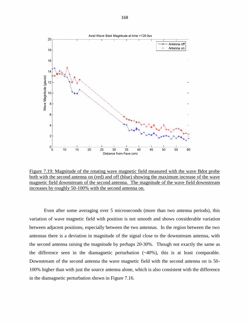
168
Figure 7.19: Magnitude of the rotating wave magnetic field measured with the wave Bdot probe
both with the second antenna on (red) and off (blue) showing the maximum increase of the wave
magnetic field downstream of the second antenna. The magnitude of the wave field downstream
increases by roughly 50-100% with the second antenna on.
Even after some averaging over 5 microseconds (more than two antenna periods), this
variation of wave magnetic field with position is not smooth and shows considerable variation
between adjacent positions, especially between the two antennas. In the region between the two
antennas there is a deviation in magnitude of the signal close to the downstream antenna, with
the second antenna raising the magnitude by perhaps 20-30%. Though not exactly the same as
the difference seen in the diamagnetic perturbation (~40%), this is at least comparable.
Downstream of the second antenna the wave magnetic field with the second antenna on is 50-
100% higher than with just the source antenna alone, which is also consistent with the difference
in the diamagnetic perturbation shown in Figure 7.16.
169
The increase of 50-100% to the wave magnitude downstream of the second antenna
within one wavelength of the second antenna suggests that the additional antenna was able to
drive a plasma wave further downstream than with just the source antenna by itself, suggesting
that additional wave power added downstream of the plasma source can make a significant
contribution to the wave and particle population downstream of the source.
The above results were obtained after working to get the two antennas oscillating in
phase at the same frequency. But despite these efforts, the second antenna would only load
repeatedly for a short period of time, and in this period the two antennas were not exactly in
phase with each other. The following section describes an attempt to drive the second antenna at
a lower frequency than the source but near half the source frequency, so that one antenna would
be operating near a harmonic of the other.
Section 7.10: Operation of the Downstream Antenna at Lower Frequency
While the source antenna and downstream antenna were both operated near 630 kHz for
the previous results in this chapter, here the downstream antenna was re-tuned to oscillate at
~300 kHz. This was done by altering the tuning capacitors in the antenna power supply, but due
to a limitation on the supply size and the number of capacitors available, the frequency is not
precisely half that of the source antenna power supply. Despite this, operating the second
antenna at the lower frequency allowed for a repeatable loading profile for much longer than was
possible for the higher frequency case. This loading profile is shown below in Figure 7.20:

170
Figure 7.20: Loading profile of the downstream antenna when operated at the lower frequency
(~300 kHz) compared to the source antenna for the whole 400 microseconds that the source
antenna is active.
In order to compare with the data from the previous section which was operated for only
a short period (~160 microseconds), measurements were also taken with the second antenna
oscillating at the lower frequency but only at the same times that the higher frequency antenna
was operated, this loading profile is shown below in Figure 7.21:
DS Antenna on for whole Shot
-4.00E+02
-3.00E+02
-2.00E+02
-1.00E+02
0.00E+00
1.00E+02
2.00E+02
3.00E+02
4.00E+02
0.00E+00 1.00E-04 2.00E-04 3.00E-04 4.00E-04 5.00E-04 6.00E-04
Time (microseconds)
DS
An
ten
na C
urr
en
t (A
)

171
Figure 7.21: Loading profile of the downstream antenna when operated at the lower frequency
(~300 kHz) compared to the source antenna for the short pulse period to compare with the results
in sections 7.5-7.9, when the second antenna is only on for a short time.
In both of these loading profiles, the current oscillating in the downstream antenna is
comparable with the higher frequency case during the 160 microseconds it was on, but the
downstream antenna in the lower frequency case oscillated at a higher current before and after
this time.
When the antenna is operated at the 365 kHz frequency roughly the same number of total
ions are arriving at the downstream RFA, but there is a significant drop in the number of higher
energy ions arriving compared to the high frequency case. At this point in the shot there is not a
significant difference between the two low frequency profiles, suggesting that turning on the
second antenna earlier did not have a large contribution to the peak plasma population. Taking
the derivative of the curves and making the same assumptions as before, the ion velocity
distribution is plotted below in Figure 7.22:
Comparison with Higher Frequency
-4.00E+02
-3.00E+02
-2.00E+02
-1.00E+02
0.00E+00
1.00E+02
2.00E+02
3.00E+02
4.00E+02
0.00E+00 1.00E-04 2.00E-04 3.00E-04 4.00E-04 5.00E-04 6.00E-04
Time (microseconds)
DS
An
ten
na C
urr
en
t (A
)

172
Figure 7.22: Ion velocity distribution functions measured by the RFA for the cases of the second
antenna turned off (black), operated at the same frequency as the source antenna for the short
pulse (red), operated at roughly half the frequency of the source antenna for a short pulse (green),
and operated at half the frequency of the source antenna for the full 400 microseconds that the
source antenna is on (blue).
While the velocity distribution for the lower frequency case also appears to be a two peak
distribution, there is not as much separation between the peaks as there is in the case of the
second antenna being turned off, or operated at the higher frequency. There are an increased
number of lower energy ions seen in the lower frequency case than with the antenna off, as well
as more high energy ions. This is discussed further in the following section.
Section 7.11: Ion Energy Populations and Comparison of Antenna Power:
In the previous section when the ion energy distributions were presented, it was at a
characteristic time near the peak signal of the downstream RFA (~109 cm downstream of the

173
source). In order to look at the total population of ions moving downstream, the following series
of plots are the energy flux of ions within a particular velocity range:
Figure 7.23: 15-20 km/s, the bulk of the accelerated plasma
Figure 7.24: >20 km/s, the low density, higher energy portion
Figure 7.25: 5-10 km/s, the slower population seen with low frequency antenna
arriving at the detector as a function of time, giving information on whether each antenna
configuration is slowing down or speeding up particles. The magnitude of the signal is the sum
of the directed kinetic energy arriving at the collector.
Looking at the higher velocity components of the population, which represent the bulk of
the energy arriving at the detector, the higher frequency second antenna is dominant during the
time the antenna is on.
Figure 7.23: Ions with velocity 15-20 km/s received at the downstream RFA as a function of
time for the four downstream antenna configurations considered.

174
For the ions travelling 15-20 km/s there is an exaggerated case of the high frequency
second antenna increasing the energy of the particles downstream by more than a factor of two,
while there is less of an increase for the case of the lower frequency antenna. The ions with
velocities 10-20 km/s represent the bulk of the kinetic energy arriving at the detector downstream
~80%, and there is a definite advantage of the high frequency antenna over the lower frequency
antenna (in terms of operating the downstream antenna. When looking at the highest velocity
ions:
Figure 7.24: Ions with velocity >20 km/s received at the downstream RFA as a function of time
for the four downstream antenna configurations considered.
there is a comparable burst of high velocity ions (>20 km/s) early in time for the lower frequency
antenna and the source antenna by itself, it’s only the case of the higher frequency downstream
antenna that a significant number of high velocity ions are contributing to the energy flux later in
time during the bulk of the plasma flow. This suggests that the lower frequency antenna

175
configuration is less suited to producing higher velocity ions to carry the energy flux downstream
compared to more low energy ions.
To further illustrate this, we consider the lower velocity populations such as below in
Figure 7.25:
Figure 7.25: Ions with velocity 5-10 km/s received at the downstream RFA as a function of time
for the four downstream antenna configurations considered.
where it is seen that the lower frequency antenna is putting more energy into lower velocity
particles than the higher frequency configuration. The amount of energy coming from these
lower velocity particles is only ~10% of the total energy flux.
While the second antenna is on, there is a dramatic increase in the amount of energy
arriving at the collector in the form of the directed energy of ions, as seen in the large increase
from 150 microseconds to 225 microseconds. The higher frequency downstream antenna has the
largest contribution during this period. Later in time this is no longer the case, with the higher

176
frequency second antenna dropping to the lowest of the four. This is the result of differing
contributions between low velocity and high velocity ions to the total energy arriving at the
detector. Before moving into the narrower velocity ranges, it is interesting to compare the total
energy received at the collector over the entire shot for the different configurations compared to
having the second antenna off (source antenna by itself).
160 microsecond pulse, 630 kHz (same as source antenna): ~32.9% increase
160 microsecond pulse, 365 kHz (roughly half the source): ~23.3% increase
400 microsecond pulse, 365 kHz (roughly half the source): ~33.6% increase
It is interesting to note that the lower frequency antenna needed to be operated for a much longer
time to result in a comparable increase in the downstream kinetic energy of the particles.
To summarize, the high frequency configuration (in which the downstream antenna
matches the source antenna frequency) puts more of its energy into the higher velocity ions
which arrive earlier with the bulk of the plasma pulse, and seems to be the only configuration
that can produce a significant amount of ions with velocity above 20 km/s later in time. In
contrast, the lower frequency configuration puts more of its energy into the lower velocity
particles of which some arrive much later in time and with the extended shot length can continue
to put energy into ions with velocities below 20 km/s later in time after the bulk of the plasma
has moved downstream. This requires the lower frequency configuration to be on for a longer
period of time to achieve the same increase in the energy flux of the ions, while the higher
frequency configuration puts most of its energy into high velocity ions during the short period
when the bulk of the plasma is near or inside the downstream antenna. This partly explains why
the ion velocity distribution for the lower frequency configuration has more fast ions than the
source antenna alone, but also more slow ions than the source antenna by itself. At the same
time, the higher frequency configuration is nearly just a shift upwards in ion velocity compared
to the source antenna alone.
To get a rough idea of how much additional energy needed to be supplied to the
experiment to account for this ~33% increase in energy flux with the second antenna
downstream, we can compare the current oscillating in the source antenna relative to the

177
downstream antenna when they were being driven at the same frequency. The measured
inductances of the two antenna coils were measured to be comparable, with the source antenna at
~0.848 microhenries and the larger downstream antenna at ~0.936 microhenries (the difference
is a combination of the size of the antenna compared with shape of the coil legs). When
comparing the energy flowing into each inductor to sustain that current, we can come up with a
rough estimate of how much additional power needed to be supplied to run two antennas in place
of one.
Comparing the two loading profiles (Figures 7.9 and 7.10) during the 160 microseconds
that the second antenna is on suggests an estimated 29.2% increase in power while the
downstream antenna is in operation. The second antenna is not expected to contribute to the
ionization of particles, so the power oscillating in the downstream antenna is expected to directly
contribute the driving of the plasma wave and the acceleration of particles. This 29.2% increase
in power into the system is roughly approximate to the 32.9% in ion energy flux observed
downstream. One possible explanation for this is that the source antenna spends the bulk of its
power in the first 80-90 microseconds just ionizing the plasma particles and accelerating them
out of the source region and up to ~6.5 km/s (as discussed in Chapter 5). Then over the next
~200 microseconds the power of the source antenna went mostly into accelerating the bulk of the
plasma ions up to a higher velocity and increasing the energy flux of the ions. Turning on the
second antenna during this time period directly contributed to this effect, getting an increase in
downstream ion flux roughly equivalent to the power going into the second antenna. The
increase in the diamagnetic perturbation along the axis and the wave magnetic field suggests, just
as in Chapters 4 and 5, that these are connected to the acceleration of the plasma downstream of
the source antenna.
Unlike the results in the earlier chapters, we now have a comparison with a lower
frequency antenna configuration of roughly the same power. Comparing the antenna current in
the loading profile of Figure 7.21 to the source antenna in the same fashion of above, we can
estimate that operating the second downstream antenna in the lower frequency configuration is
an increase in power of ~30.5% for the 160 microseconds that it is on, but for only a ~23.3%
increase in downstream ion energy flux. This is the result of the lower frequency configuration
putting more of its energy into larger numbers of lower velocity ions than in the smaller numbers

178
of high velocity particles. The result is that the lower frequency mode is less effective than the
higher frequency mode in this case at building up the kinetic energy of the ions downstream even
for the same amount of input power. Note that it does not decrease by a factor of 2 even though
the frequency has decreased by almost half, so there is still not a simple dependence on
frequency. The end result of a broader velocity distribution with the antenna in the lower
frequency mode could mean that the damping mechanism is more pronounced in the lower
frequency case, leading to a higher temperature in the directed energy of the ions.
So while the variation of power and frequency of the source antenna in section 7.2
suggested that input power was the dominant factor in producing the energetic plasma beam with
the frequency dependence not being obvious, these results suggest that power and frequency of
the antenna have a direct effect on the ion energy flux downstream and the ion velocity
distribution, with the higher frequency being more effective.
Section 7.12: Limitations of the Downstream Antenna and Proposed Improvements
The most severe limitation in introducing more power into the system with a second
antenna was getting the downstream antenna and the source antenna to work in concert to result
in a consistently accelerated plasma population. The solution for this problem was to either only
fire the downstream antenna for a short period while there was a dense plasma population
connecting the two antennas, or to lower the frequency of the downstream antenna to roughly
half that of the source antenna. Both of these solutions resulted in an improvement in the energy
flux downstream and an increase in higher velocity ions, but the lower frequency antenna
configuration resulted in less of a performance increase by making an increased number of
slower ions as well as faster ions.
The limitation of only firing the second antenna when there is a dense plasma connecting
the source antenna with the downstream antenna requires a dramatic improvement in the feeding
of the source antenna in order to sustain that rate of flow for a longer period of time. The
method described in Chapter 2 of letting neutral gas flow into the source through a tube at the
thermal speed of the gas is inadequate for this task, which limited the effective shot length to
~240 microseconds. To improve on this requires a method of increasing the neutral flux into the

179
source region to sustain this effect over a longer time period, or a way to make repeatable pulses
of neutrals into the source with the antenna system only being active during those periods, to
maximize the effectiveness of the pulses.
Similarly, increasing both the power and frequency of the antennas are expected to result
in an improvement based on the modifications that were made to the system. The most effective
way to increase the performance would be to increase the power coupled from the antenna to the
plasma, while keeping the frequency the same or higher than in these results.
Together with the intense diamagnetic perturbations discussed earlier, these results
indicate that increasing the amount of power into the downstream plasma results in a more
extended diamagnetic perturbation and overall significant improvement in terms of exhaust
velocity for the plasma and collimation of the beam. The presence of a large diamagnetic
perturbation (and in some cases a diamagnetic cavity near the axis), suggests that this experiment
can demonstrate some high beta plasma effects that are likely to be observed in space operation
of a thruster, but are typically not seen in laboratory experiments of this type.

180
Cited References:
[1] Sutton, Rocket Propulsion Elements, Wiley-Interscience, 2000
[2] Prager, Experimental investigation of plasma downstream of a high power helicon, Thesis
(Ph. D.)--University of Washington, 2008
[3] Chen, Physics of Plasmas Vol 1, Springer, 2006
[4] Hutchinson, Principles of Plasma Diagnostics, Cambride University Press, 2002
[5] Sovey, NASA SOLAR ELECTRIC PROPULSION TECHNOLOGY APPLICATION
READINESS (NSTAR) http://www.grc.nasa.gov/WWW/ion/past/90s/nstar.htm
[6] Snecma, PPS®1350-G SPACE PROPULSION STATIONARY PLASMA THRUSTER,
http://www.snecma.com/IMG/files/fiche_pps1350g_ang_2011_modulvoir_file_fr.pdf
[7] Winglee, Simulation and laboratory validation of magnetic nozzle effects for the high power
helicon thruster, PHYSICS OF PLASMAS 14, 063501, 2007
[8] Ziemba, Plasma characteristics of a high power helicon discharge, Plasma Sources Sci.
Technol. 15 (2006) 517–525
[9] Ziemba, Experimental investigation of the mini-magnetospheric plasma propulsion
prototype, Thesis (Ph. D.)--University of Washington, 2003
[10] Prager, Ion energy characteristics downstream of a high power helicon, Plasma Sources Sci.
Technol. 17 (2008) 025003 (12pp)
[11] Prager, Wave propagation downstream of a high power helicon in a dipolelike magnetic
field, PHYSICS OF PLASMAS 17, 013504, 2010
[12] Chen, Generalized theory of helicon waves. I. Normal modes, Phys. Plasmas 4 (9),
September 1997
[13] Boswell, Very efficient plasma generation by whistler waves near the lower hybrid
frequency, 1984 Plasma Phys. Control. Fusion 26 1147
[14] Cassady, VASIMR Performance Results, 46th AIAA/ASME/SAE/ASEE Joint Propulsion
Conference & Exhibit 25 - 28 July 2010
[15] Miljak, Density limit in helicon discharges, Plasma Sources Sci. Technol. 7 (1998) 537–549
[16] NIST Atomic Spectra Database, http://www.nist.gov/pml/data/asd.cfm
[17] Huba, NRL PLASMA FORMULARY, Naval Research Laboratory, 2011
[18] Wessel, Plasmoid propagation in a transverse magnetic field and in a magnetized plasma,
Phys. Of Fluids, Vol. 31, No. 12, December 1988
[19] Corr, High-beta plasma effects in a low-pressure helicon plasma, PHYSICS OF PLASMAS
14, 122503, 2007

181
[20] Parks, Physics of Space Plasmas, Westview Press, 2004
[21] Stenzel, Electron magnetohydrodynamic turbulence in a high-beta plasma. I. Plasma
parameters and instability conditions, Phys. Plasmas, Vol. 7, No. 11, November 2000
[22] Banerjee, A laboratory produced extremely large beta plasma, Phys. Plasmas 13, 092503,
2006
[23] Charles, Laboratory evidence of a supersonic ion beam generated by a current-free
‘‘helicon’’ double-layer, Phys. Plasmas, Vol. 11, No. 4, April 2004
[24] Conway, Evolution of ion and electron energy distributions in pulsed helicon plasma
discharges, Plasma Sources Sci. Technol. 7 (1998) 337–347
[25] Light, Helicon wave excitation with helical antennas, Phys. Plasmas 2 (4). April 1995
[26] Choueiri, Faraday Acceleration with Radio-Frequency Assisted Discharge, JOURNAL OF
PROPULSION AND POWER Vol. 22, No. 3, May–June 2006
[27] Inutake, Generation of supersonic plasma flows using an applied-field MPD arcjet and
ICRF heating, Plasma Phys. Control. Fusion 49 (2007) A121–A134
[28] Arefiev, Ambipolar acceleration of ions in magnetic nozzle, PHYSICS OF PLASMAS 15,
042109, 2008
[29] Saka, Plasma flow characteristics in converging field line geometry in anisotropic plasmas,
Adv. Polar Upper Atmos. Res., 19, 80-83, 2005
[30] Little, The Influence of Induced Currents on Magnetic Nozzle Acceleration and Plasma
Detachment, 46th AIAA/ASME/SAE/ASEE Joint Propulsion Conference & Exhibit 25 - 28 July
2010
[31] Gilland, The effects of neutral depletion on helicon wave plasma generation, Thesis (Ph.
D.)--University of Wisconsin-Madison, 2004


