
Dr. Francisco M. Gonzalez-Longatt, [email protected] .Copyright © 2009 1/63
All
right
s re
serv
ed. N
o pa
rt of
this
pub
licat
ion
may
be
repr
oduc
ed o
r dis
tribu
ted
in a
ny fo
rm w
ithou
t per
mis
sion
of t
he a
utho
r. C
opyr
ight
© 2
009.
http
:ww
w.fg
long
att.o
rg.v
e
Francisco M. Gonzalez-Longatt, Dr.ScManchester, UK, November, 2009
Tutorial:Introduction to Modal Analysis

Dr. Francisco M. Gonzalez-Longatt, [email protected] .Copyright © 2009 2/63
All
right
s re
serv
ed. N
o pa
rt of
this
pub
licat
ion
may
be
repr
oduc
ed o
r dis
tribu
ted
in a
ny fo
rm w
ithou
t per
mis
sion
of t
he a
utho
r. C
opyr
ight
© 2
009.
http
:ww
w.fg
long
att.o
rg.v
e
This tutorial is a simple theoretical introduction to modalanalysis
Tutorial:Introduction to Modal Analysis
Francisco M. Gonzalez-Longatt, [email protected]
Manchester, 28th October 2009

Dr. Francisco M. Gonzalez-Longatt, [email protected] .Copyright © 2009 3/63
All
right
s re
serv
ed. N
o pa
rt of
this
pub
licat
ion
may
be
repr
oduc
ed o
r dis
tribu
ted
in a
ny fo
rm w
ithou
t per
mis
sion
of t
he a
utho
r. C
opyr
ight
© 2
009.
http
:ww
w.fg
long
att.o
rg.v
e
1. IntroductionIntroduction to Modal Analysis in Power
System

Dr. Francisco M. Gonzalez-Longatt, [email protected] .Copyright © 2009 4/63
All
right
s re
serv
ed. N
o pa
rt of
this
pub
licat
ion
may
be
repr
oduc
ed o
r dis
tribu
ted
in a
ny fo
rm w
ithou
t per
mis
sion
of t
he a
utho
r. C
opyr
ight
© 2
009.
http
:ww
w.fg
long
att.o
rg.v
e
1. Introduction: Small Signal Stability• Small signal stability is the ability of the power system to
maintain synchronism when subjected to smalldisturbances [1].
• A disturbance is considered to be small if the equationsthat describe the resulting response of power systemmay be linearized for the purpose of analysis.
• Instability that result can be of two forms [1]:– Steady increase in generator rotor angle due to lack
synchronizing torque,– Rotor oscillation of increasing amplitude due to lack of sufficient
damping torque.
[1] P. Kundur, Power System Stability and Control. New York: McGraw- Hill, 1994.

Dr. Francisco M. Gonzalez-Longatt, [email protected] .Copyright © 2009 5/63
All
right
s re
serv
ed. N
o pa
rt of
this
pub
licat
ion
may
be
repr
oduc
ed o
r dis
tribu
ted
in a
ny fo
rm w
ithou
t per
mis
sion
of t
he a
utho
r. C
opyr
ight
© 2
009.
http
:ww
w.fg
long
att.o
rg.v
e
1. Introduction: Small Signal Stability
Instable
• TS Negative• TDPositive
δ∆ ST∆
DT∆eT∆
ω∆δ∆
P
0 t
δ∆P
0 t
Stable• TS Positive• TDPositive
δ∆
ST∆
DT∆ eT∆
ω∆
(a) With constant field voltage
Non-oscillatory
Dr. Francisco M. Gonzalez-Longatt, [email protected] .Copyright © 2009 6/63
All
right
s re
serv
ed. N
o pa
rt of
this
pub
licat
ion
may
be
repr
oduc
ed o
r dis
tribu
ted
in a
ny fo
rm w
ithou
t per
mis
sion
of t
he a
utho
r. C
opyr
ight
© 2
009.
http
:ww
w.fg
long
att.o
rg.v
e
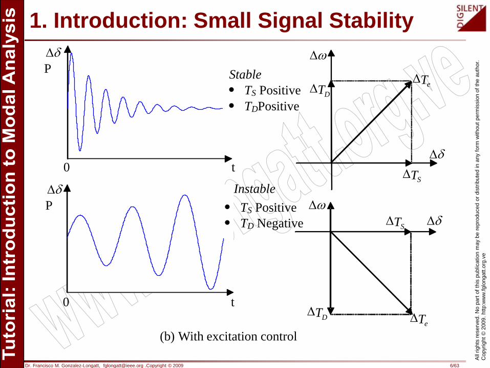
1. Introduction: Small Signal Stabilityδ∆
P
0 t
Stable• TS Positive• TDPositive
δ∆
ST∆
DT∆ eT∆
ω∆
δ∆P
0 t
Instable• TS Positive• TD Negative δ∆ST∆
DT∆eT∆
ω∆
(b) With excitation control

Dr. Francisco M. Gonzalez-Longatt, [email protected] .Copyright © 2009 7/63
All
right
s re
serv
ed. N
o pa
rt of
this
pub
licat
ion
may
be
repr
oduc
ed o
r dis
tribu
ted
in a
ny fo
rm w
ithou
t per
mis
sion
of t
he a
utho
r. C
opyr
ight
© 2
009.
http
:ww
w.fg
long
att.o
rg.v
e
1. Introduction: Small Signal Stability• ln today's practical power systems, the small-signal
stability problem is usually one of insufficient damping ofsystem oscillations.
• Small signal inherent analysis using linear techniquesprovides valuable information about the dynamiccharacteristics of the power system and assists itsdesign.

Dr. Francisco M. Gonzalez-Longatt, [email protected] .Copyright © 2009 8/63
All
right
s re
serv
ed. N
o pa
rt of
this
pub
licat
ion
may
be
repr
oduc
ed o
r dis
tribu
ted
in a
ny fo
rm w
ithou
t per
mis
sion
of t
he a
utho
r. C
opyr
ight
© 2
009.
http
:ww
w.fg
long
att.o
rg.v
e
2. Fundamental Concepts of Small
Signal Stability

Dr. Francisco M. Gonzalez-Longatt, [email protected] .Copyright © 2009 9/63
All
right
s re
serv
ed. N
o pa
rt of
this
pub
licat
ion
may
be
repr
oduc
ed o
r dis
tribu
ted
in a
ny fo
rm w
ithou
t per
mis
sion
of t
he a
utho
r. C
opyr
ight
© 2
009.
http
:ww
w.fg
long
att.o
rg.v
e
2. State-Space Representation• The behaviour of a dynamic system, such as a power
system, may be described by a set of n first order non-linear ordinary differential equations.
• This can be written using vector-matrix notation [1]:
where:( )t,,uxfx =
=
nx
xx
2
1
x
=
ru
uu
2
1
u
=
nf
ff
2
1
f

Dr. Francisco M. Gonzalez-Longatt, [email protected] .Copyright © 2009 10/63
All
right
s re
serv
ed. N
o pa
rt of
this
pub
licat
ion
may
be
repr
oduc
ed o
r dis
tribu
ted
in a
ny fo
rm w
ithou
t per
mis
sion
of t
he a
utho
r. C
opyr
ight
© 2
009.
http
:ww
w.fg
long
att.o
rg.v
e
2. State Space Representation
• The column vector x is deferred to as the state vector.• xi are referred as state variables.
The column vector u is the vector of inputs to thesystem.
• u are the external signal that influence the performanceof the system.
• t denote time• is the derivate of a state variable respect to time.
=
nx
xx
2
1
x
=
ru
uu
2
1
u
=
nf
ff
2
1
f
x

Dr. Francisco M. Gonzalez-Longatt, [email protected] .Copyright © 2009 11/63
All
right
s re
serv
ed. N
o pa
rt of
this
pub
licat
ion
may
be
repr
oduc
ed o
r dis
tribu
ted
in a
ny fo
rm w
ithou
t per
mis
sion
of t
he a
utho
r. C
opyr
ight
© 2
009.
http
:ww
w.fg
long
att.o
rg.v
e
2. State Space Representation• The system is called autonomous if the derivatives of
the stated variables are not explicit functions of time.
• The output variables can be observed in the system.• These may be expressed in terms of the state variables
and the inputs variables [1]:
• where:
( )uxfx ,=
( )uxgy ,=
=
my
yy
2
1
y
=
rg
gg
2
1
g

Dr. Francisco M. Gonzalez-Longatt, [email protected] .Copyright © 2009 12/63
All
right
s re
serv
ed. N
o pa
rt of
this
pub
licat
ion
may
be
repr
oduc
ed o
r dis
tribu
ted
in a
ny fo
rm w
ithou
t per
mis
sion
of t
he a
utho
r. C
opyr
ight
© 2
009.
http
:ww
w.fg
long
att.o
rg.v
e
2. State Space Representation
• The column vector y is the vector of outputs• g is a vector of non-linear factions relating state and
input variables to output variables.
=
my
yy
2
1
y
=
rg
gg
2
1
g

Dr. Francisco M. Gonzalez-Longatt, [email protected] .Copyright © 2009 13/63
All
right
s re
serv
ed. N
o pa
rt of
this
pub
licat
ion
may
be
repr
oduc
ed o
r dis
tribu
ted
in a
ny fo
rm w
ithou
t per
mis
sion
of t
he a
utho
r. C
opyr
ight
© 2
009.
http
:ww
w.fg
long
att.o
rg.v
e
2.1. State Concept• The concept of state is fundamental to the state-space
approach.• The state of a system represents the minimum amount
of information about the system at any instant in time t0that is necessary so that its future behaviour can bedetermined without the input before t0.
• Any set of n linearly independent system variables maybe used to describe the state of the system –statevariables [1].
• State variables form a minimal set of dynamic variablesthat, along with the inputs to the system, provide acomplete description of the system behaviour

Dr. Francisco M. Gonzalez-Longatt, [email protected] .Copyright © 2009 14/63
All
right
s re
serv
ed. N
o pa
rt of
this
pub
licat
ion
may
be
repr
oduc
ed o
r dis
tribu
ted
in a
ny fo
rm w
ithou
t per
mis
sion
of t
he a
utho
r. C
opyr
ight
© 2
009.
http
:ww
w.fg
long
att.o
rg.v
e
2.1. State-Space Concept• The system state may be represented in a n-dimensional
Euclidean space, called state space.

Dr. Francisco M. Gonzalez-Longatt, [email protected] .Copyright © 2009 15/63
All
right
s re
serv
ed. N
o pa
rt of
this
pub
licat
ion
may
be
repr
oduc
ed o
r dis
tribu
ted
in a
ny fo
rm w
ithou
t per
mis
sion
of t
he a
utho
r. C
opyr
ight
© 2
009.
http
:ww
w.fg
long
att.o
rg.v
e
2.2. Equilibrium (or singular) points• Those points where all derivatives of state variables are
simultaneously zero [1].
• They define the points on the trajectory with zerovelocity.
• This system is at rest since all the variables are constantand unvarying with time.
=
==
=
0
00
2
1
nx
xx
x

Dr. Francisco M. Gonzalez-Longatt, [email protected] .Copyright © 2009 16/63
All
right
s re
serv
ed. N
o pa
rt of
this
pub
licat
ion
may
be
repr
oduc
ed o
r dis
tribu
ted
in a
ny fo
rm w
ithou
t per
mis
sion
of t
he a
utho
r. C
opyr
ight
© 2
009.
http
:ww
w.fg
long
att.o
rg.v
e
2.2. Equilibrium (or singular) points• The equilibrium or singular point must therefore satisfy
the equation:
where x0 is the state vecto x at the equilibrium point.
( ) 00 0 === xfx

Dr. Francisco M. Gonzalez-Longatt, [email protected] .Copyright © 2009 17/63
All
right
s re
serv
ed. N
o pa
rt of
this
pub
licat
ion
may
be
repr
oduc
ed o
r dis
tribu
ted
in a
ny fo
rm w
ithou
t per
mis
sion
of t
he a
utho
r. C
opyr
ight
© 2
009.
http
:ww
w.fg
long
att.o
rg.v
e
2.3. Stability of a Dynamic System• Linear system: stability is entirely independent of the
input.• State of a stable system with zero input will always
return to the origin of the state space, independent of thefinite initial state.
• Non-linear system: Stability depends on the type andmagnitude of input and the initial state.

Dr. Francisco M. Gonzalez-Longatt, [email protected] .Copyright © 2009 18/63
All
right
s re
serv
ed. N
o pa
rt of
this
pub
licat
ion
may
be
repr
oduc
ed o
r dis
tribu
ted
in a
ny fo
rm w
ithou
t per
mis
sion
of t
he a
utho
r. C
opyr
ight
© 2
009.
http
:ww
w.fg
long
att.o
rg.v
e
2.4. Classification of Stability• Classification of stability of non-linear system, depending
on the region of state space in which the state vectorranges:– Local stability or stability in the small.– Finite stability.– Global stability or stability large.

Dr. Francisco M. Gonzalez-Longatt, [email protected] .Copyright © 2009 19/63
All
right
s re
serv
ed. N
o pa
rt of
this
pub
licat
ion
may
be
repr
oduc
ed o
r dis
tribu
ted
in a
ny fo
rm w
ithou
t per
mis
sion
of t
he a
utho
r. C
opyr
ight
© 2
009.
http
:ww
w.fg
long
att.o
rg.v
e
2.4.a. Local Stability
• The system is locally stable about equilibrium point if,when subjected to small perturbation, it remain within asmall region surrounding the equilibrium point.
• If, a t increase, the system return to the original state, itis said to be asymptotically stable in the small.

Dr. Francisco M. Gonzalez-Longatt, [email protected] .Copyright © 2009 20/63
All
right
s re
serv
ed. N
o pa
rt of
this
pub
licat
ion
may
be
repr
oduc
ed o
r dis
tribu
ted
in a
ny fo
rm w
ithou
t per
mis
sion
of t
he a
utho
r. C
opyr
ight
© 2
009.
http
:ww
w.fg
long
att.o
rg.v
e
2.4.b. Finite Stability
• If the state of a system remains within a finite region R, itis said to be stable within R.
• If, further, the state of the system returns to the originalequilibrium point form any point within R, it isasymptotically stable within the finite region R.

Dr. Francisco M. Gonzalez-Longatt, [email protected] .Copyright © 2009 21/63
All
right
s re
serv
ed. N
o pa
rt of
this
pub
licat
ion
may
be
repr
oduc
ed o
r dis
tribu
ted
in a
ny fo
rm w
ithou
t per
mis
sion
of t
he a
utho
r. C
opyr
ight
© 2
009.
http
:ww
w.fg
long
att.o
rg.v
e
2.4.c. Global Stability
• The system is said to be globally stable if R include theentire finite space.

Dr. Francisco M. Gonzalez-Longatt, [email protected] .Copyright © 2009 22/63
All
right
s re
serv
ed. N
o pa
rt of
this
pub
licat
ion
may
be
repr
oduc
ed o
r dis
tribu
ted
in a
ny fo
rm w
ithou
t per
mis
sion
of t
he a
utho
r. C
opyr
ight
© 2
009.
http
:ww
w.fg
long
att.o
rg.v
e
3. Linealization
Dr. Francisco M. Gonzalez-Longatt, [email protected] .Copyright © 2009 23/63
All
right
s re
serv
ed. N
o pa
rt of
this
pub
licat
ion
may
be
repr
oduc
ed o
r dis
tribu
ted
in a
ny fo
rm w
ithou
t per
mis
sion
of t
he a
utho
r. C
opyr
ight
© 2
009.
http
:ww
w.fg
long
att.o
rg.v
e
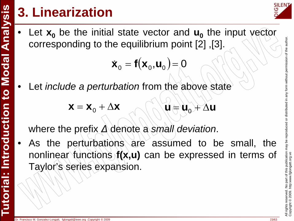
3. Linearization• Let x0 be the initial state vector and u0 the input vector
corresponding to the equilibrium point [2] ,[3].
• Let include a perturbation from the above state
where the prefix Δ denote a small deviation.• As the perturbations are assumed to be small, the
nonlinear functions f(x,u) can be expressed in terms ofTaylor’s series expansion.
( ) 0, 000 == uxfx
xxx ∆+= 0 uuu ∆+= 0
Dr. Francisco M. Gonzalez-Longatt, [email protected] .Copyright © 2009 24/63
All
right
s re
serv
ed. N
o pa
rt of
this
pub
licat
ion
may
be
repr
oduc
ed o
r dis
tribu
ted
in a
ny fo
rm w
ithou
t per
mis
sion
of t
he a
utho
r. C
opyr
ight
© 2
009.
http
:ww
w.fg
long
att.o
rg.v
e
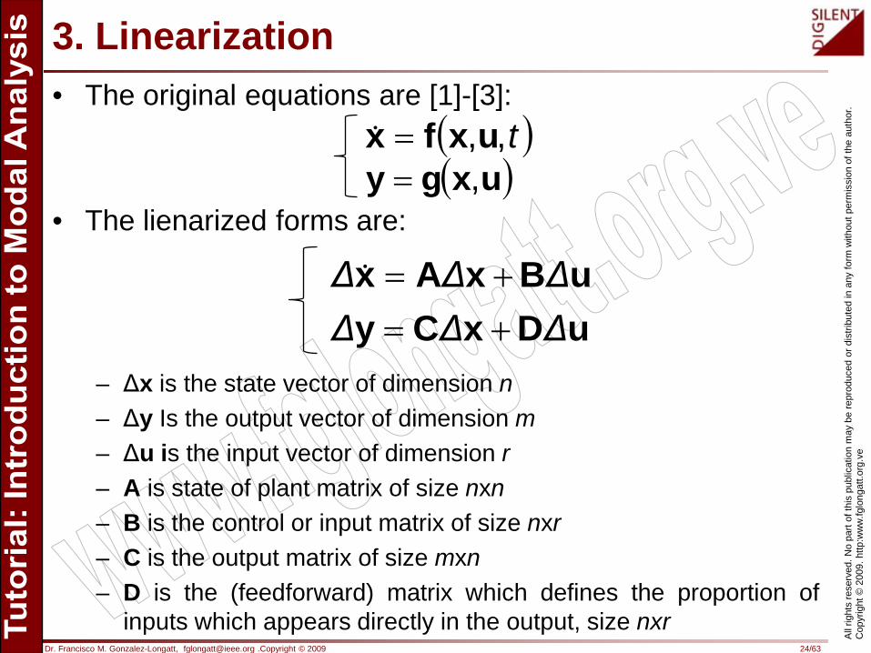
3. Linearization• The original equations are [1]-[3]:
• The lienarized forms are:
– Δx is the state vector of dimension n– Δy Is the output vector of dimension m– Δu is the input vector of dimension r– A is state of plant matrix of size nxn– B is the control or input matrix of size nxr– C is the output matrix of size mxn– D is the (feedforward) matrix which defines the proportion of
inputs which appears directly in the output, size nxr
( )t,,uxfx =( )uxgy ,=
uDxCyuBxAx
ΔΔΔΔΔΔ
+=+=
Dr. Francisco M. Gonzalez-Longatt, [email protected] .Copyright © 2009 25/63
All
right
s re
serv
ed. N
o pa
rt of
this
pub
licat
ion
may
be
repr
oduc
ed o
r dis
tribu
ted
in a
ny fo
rm w
ithou
t per
mis
sion
of t
he a
utho
r. C
opyr
ight
© 2
009.
http
:ww
w.fg
long
att.o
rg.v
e
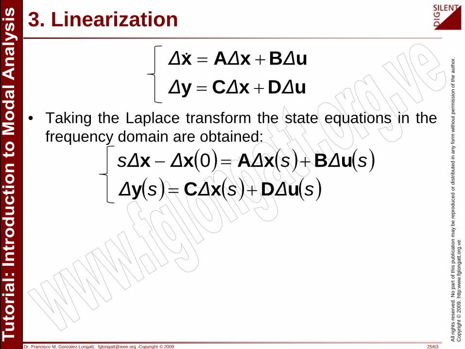
3. Linearization
• Taking the Laplace transform the state equations in thefrequency domain are obtained:
uDxCyuBxAx
ΔΔΔΔΔΔ
+=+=
( ) ( ) ( )( ) ( ) ( )sΔsΔsΔ
sΔsΔΔsΔuDxCy
uBxAxx+=
+=− 0

Dr. Francisco M. Gonzalez-Longatt, [email protected] .Copyright © 2009 26/63
All
right
s re
serv
ed. N
o pa
rt of
this
pub
licat
ion
may
be
repr
oduc
ed o
r dis
tribu
ted
in a
ny fo
rm w
ithou
t per
mis
sion
of t
he a
utho
r. C
opyr
ight
© 2
009.
http
:ww
w.fg
long
att.o
rg.v
e
3. Linearization• Block diagram of the state-space representation [1]-[3]
B
D
Is1
A
ΣΣ Cu∆ y∆x∆x∆ +
+
++

Dr. Francisco M. Gonzalez-Longatt, [email protected] .Copyright © 2009 27/63
All
right
s re
serv
ed. N
o pa
rt of
this
pub
licat
ion
may
be
repr
oduc
ed o
r dis
tribu
ted
in a
ny fo
rm w
ithou
t per
mis
sion
of t
he a
utho
r. C
opyr
ight
© 2
009.
http
:ww
w.fg
long
att.o
rg.v
e
3. Linearization• The initial conditions are Δx(0) assumed zero.• The solution of the state equations can be obtained [1]:
• The Laplace transform of Δx and Δy are seen to havetwo components:
(i) Dependent on the initial conditions and(ii) Dependent on the inputs.
• These are the Laplace transforms of the free and zero-state components of the state and output vectors
( ) ( )( ) ( ) ( )[ ] ( )sΔsΔΔssadjsΔ uDuBx
AIAICy ++
−−
= 0det

Dr. Francisco M. Gonzalez-Longatt, [email protected] .Copyright © 2009 28/63
All
right
s re
serv
ed. N
o pa
rt of
this
pub
licat
ion
may
be
repr
oduc
ed o
r dis
tribu
ted
in a
ny fo
rm w
ithou
t per
mis
sion
of t
he a
utho
r. C
opyr
ight
© 2
009.
http
:ww
w.fg
long
att.o
rg.v
e
3. Linearization• The poles of Δx and Δy are the roots of the equation:
• The values of s which satisfy this conditions are knownas eigenvalues of matrix A [1]-[3].
• The equation [1],[2]:
is referred as he characteristic equation of matrix A.
( ) 0det =− AIs
( ) 0det =− AIs

Dr. Francisco M. Gonzalez-Longatt, [email protected] .Copyright © 2009 29/63
All
right
s re
serv
ed. N
o pa
rt of
this
pub
licat
ion
may
be
repr
oduc
ed o
r dis
tribu
ted
in a
ny fo
rm w
ithou
t per
mis
sion
of t
he a
utho
r. C
opyr
ight
© 2
009.
http
:ww
w.fg
long
att.o
rg.v
e
4. Eigenvalues and Eigenvectors

Dr. Francisco M. Gonzalez-Longatt, [email protected] .Copyright © 2009 30/63
All
right
s re
serv
ed. N
o pa
rt of
this
pub
licat
ion
may
be
repr
oduc
ed o
r dis
tribu
ted
in a
ny fo
rm w
ithou
t per
mis
sion
of t
he a
utho
r. C
opyr
ight
© 2
009.
http
:ww
w.fg
long
att.o
rg.v
e
4. Eigenvalues• The eigenvalues of a matrix are given by the values of
the scalar parameter which there exist non-trivialsolutions to the equation [1]:
• For a non-trivial solution [2]:
• Expansion of the determinant give the characteristicequation.
• The n solution of λ = λ1, λ2, …λn are the eigenvalues of A[2].
( ) 0det =− AIs
( ) 0=− φλIA
Dr. Francisco M. Gonzalez-Longatt, [email protected] .Copyright © 2009 31/63
All
right
s re
serv
ed. N
o pa
rt of
this
pub
licat
ion
may
be
repr
oduc
ed o
r dis
tribu
ted
in a
ny fo
rm w
ithou
t per
mis
sion
of t
he a
utho
r. C
opyr
ight
© 2
009.
http
:ww
w.fg
long
att.o
rg.v
e
4. Eigenvectors• For every eigenvalue λi, there is an eigenvector ϕi which
satisfies:
• ϕi is called the right eigenvector of the state matrix Aassociated with the eigenvalue λi.
• Each right eigenvector is a column vector with the lengthequal to the number of the states.
• The right eigenvector is called mode shape.
iii φλφ =A

Dr. Francisco M. Gonzalez-Longatt, [email protected] .Copyright © 2009 32/63
All
right
s re
serv
ed. N
o pa
rt of
this
pub
licat
ion
may
be
repr
oduc
ed o
r dis
tribu
ted
in a
ny fo
rm w
ithou
t per
mis
sion
of t
he a
utho
r. C
opyr
ight
© 2
009.
http
:ww
w.fg
long
att.o
rg.v
e
4. Eigenvectors• Left eigenvector associated with the eigenvalue λi is the
n-row vector which satisfies:
• The right eigenvector describes how each mode ofoscillation is distributed among the system states.
• It indicates on which system variables the mode ismore observable.
• The left eigenvector, together with the system’s initialstate, determines the amplitude of the mode.
• A left eigenvector carries mode controllabilityinformation.
iii ψλψ =A

Dr. Francisco M. Gonzalez-Longatt, [email protected] .Copyright © 2009 33/63
All
right
s re
serv
ed. N
o pa
rt of
this
pub
licat
ion
may
be
repr
oduc
ed o
r dis
tribu
ted
in a
ny fo
rm w
ithou
t per
mis
sion
of t
he a
utho
r. C
opyr
ight
© 2
009.
http
:ww
w.fg
long
att.o
rg.v
e
4. Eigenvectors
The left eigenvector indicates on which systemvariables the mode is more observable.
The right eigenvector is called mode shape.

Dr. Francisco M. Gonzalez-Longatt, [email protected] .Copyright © 2009 34/63
All
right
s re
serv
ed. N
o pa
rt of
this
pub
licat
ion
may
be
repr
oduc
ed o
r dis
tribu
ted
in a
ny fo
rm w
ithou
t per
mis
sion
of t
he a
utho
r. C
opyr
ight
© 2
009.
http
:ww
w.fg
long
att.o
rg.v
e
5. Eigenvalues and stability

Dr. Francisco M. Gonzalez-Longatt, [email protected] .Copyright © 2009 35/63
All
right
s re
serv
ed. N
o pa
rt of
this
pub
licat
ion
may
be
repr
oduc
ed o
r dis
tribu
ted
in a
ny fo
rm w
ithou
t per
mis
sion
of t
he a
utho
r. C
opyr
ight
© 2
009.
http
:ww
w.fg
long
att.o
rg.v
e
5. Eigenvalues and Stability• The stability of the system is determined by the
eigenvalues λi.
• Real eigenvalues: Non oscillatory mode.– Negative real eigenvalue represent a decaying mode.– Magnitude define the decay.– Positive real eigenvalues represent aperiodic instability.
• Complex eigenvalues: Occurs in conjugate pair, andeach pairs correspond a oscillatory mode.
Dr. Francisco M. Gonzalez-Longatt, [email protected] .Copyright © 2009 36/63
All
right
s re
serv
ed. N
o pa
rt of
this
pub
licat
ion
may
be
repr
oduc
ed o
r dis
tribu
ted
in a
ny fo
rm w
ithou
t per
mis
sion
of t
he a
utho
r. C
opyr
ight
© 2
009.
http
:ww
w.fg
long
att.o
rg.v
e
5. Eigenvalues and Stability• For a complex pairs of eigenvalues [1]:
• The frequency of oscillation (f) in Hz is given by [1]:
• This represents the actual or damped frequency (f).• T he damping ratio (ζ) is given by:
• The damping ratio ζ determines the rate of decay of theamplitude of the oscillation [1]-[2].
ωσλ j±=
πω2
=f
22 ωσσς+
−=

Dr. Francisco M. Gonzalez-Longatt, [email protected] .Copyright © 2009 37/63
All
right
s re
serv
ed. N
o pa
rt of
this
pub
licat
ion
may
be
repr
oduc
ed o
r dis
tribu
ted
in a
ny fo
rm w
ithou
t per
mis
sion
of t
he a
utho
r. C
opyr
ight
© 2
009.
http
:ww
w.fg
long
att.o
rg.v
e
5. Eigenvalues and Stability
σ
ωjX
X
z1
z2(a) Stable focus
Eigenvaluesωσλ j±=
Trajectory Type of singularity
(b) Unstable focusσ
ωjX
X
z1
z2

Dr. Francisco M. Gonzalez-Longatt, [email protected] .Copyright © 2009 38/63
All
right
s re
serv
ed. N
o pa
rt of
this
pub
licat
ion
may
be
repr
oduc
ed o
r dis
tribu
ted
in a
ny fo
rm w
ithou
t per
mis
sion
of t
he a
utho
r. C
opyr
ight
© 2
009.
http
:ww
w.fg
long
att.o
rg.v
e
5. Eigenvalues and Stability
(f) Vortex
Eigenvaluesωσλ j±=
Trajectory Type of singularity
(g) Saddle
σ
ωj
X
X
z1
z2
σ
ωj
XX
z1
z2

Dr. Francisco M. Gonzalez-Longatt, [email protected] .Copyright © 2009 39/63
All
right
s re
serv
ed. N
o pa
rt of
this
pub
licat
ion
may
be
repr
oduc
ed o
r dis
tribu
ted
in a
ny fo
rm w
ithou
t per
mis
sion
of t
he a
utho
r. C
opyr
ight
© 2
009.
http
:ww
w.fg
long
att.o
rg.v
e
5. Eigenvalues and Stability
(c) Stable focus
Eigenvaluesωσλ j±=
Trajectory Type of singularity
(d) Unstable focusσ
ωj
XX
z1
z2
σ
ωj
XX
z1
z2

Dr. Francisco M. Gonzalez-Longatt, [email protected] .Copyright © 2009 40/63
All
right
s re
serv
ed. N
o pa
rt of
this
pub
licat
ion
may
be
repr
oduc
ed o
r dis
tribu
ted
in a
ny fo
rm w
ithou
t per
mis
sion
of t
he a
utho
r. C
opyr
ight
© 2
009.
http
:ww
w.fg
long
att.o
rg.v
e
6. Indexes

Dr. Francisco M. Gonzalez-Longatt, [email protected] .Copyright © 2009 41/63
All
right
s re
serv
ed. N
o pa
rt of
this
pub
licat
ion
may
be
repr
oduc
ed o
r dis
tribu
ted
in a
ny fo
rm w
ithou
t per
mis
sion
of t
he a
utho
r. C
opyr
ight
© 2
009.
http
:ww
w.fg
long
att.o
rg.v
e
6. Indexes• Numerous indices, can be calculated from eigenvectors
such as [4]:
– Participation factors,– Transfer function residues and– Mode sensitivities.
• Those are very useful in system analysis and controllerdesign.

Dr. Francisco M. Gonzalez-Longatt, [email protected] .Copyright © 2009 42/63
All
right
s re
serv
ed. N
o pa
rt of
this
pub
licat
ion
may
be
repr
oduc
ed o
r dis
tribu
ted
in a
ny fo
rm w
ithou
t per
mis
sion
of t
he a
utho
r. C
opyr
ight
© 2
009.
http
:ww
w.fg
long
att.o
rg.v
e
6.1. Participation factors• The Participation matrix (P), combine the right and left
eigenvectors [1]:
where
where ψki is the kth element in the ith row of the the lefteigenvector ψi, and φki is the kth element in the ith columnof the right eigenvector φi [4].
[ ]npppP 21=
=
=
nini
ii
ii
ni
i
i
p
pp
ψφ
ψφψφ
22
11
2
1
1p

Dr. Francisco M. Gonzalez-Longatt, [email protected] .Copyright © 2009 43/63
All
right
s re
serv
ed. N
o pa
rt of
this
pub
licat
ion
may
be
repr
oduc
ed o
r dis
tribu
ted
in a
ny fo
rm w
ithou
t per
mis
sion
of t
he a
utho
r. C
opyr
ight
© 2
009.
http
:ww
w.fg
long
att.o
rg.v
e
6.1. Participation factors• The participation factor pki is a measure of the relative
participation of the kth state variable in the ith mode, andvice versa.
• The sensitivity of a particular eigenvalue λi to thechanges in the diagonal elements of the state matrix A.
kikikip ψφ=
kk
iki a
p∂∂
=λ
kikikip ψφ=

Dr. Francisco M. Gonzalez-Longatt, [email protected] .Copyright © 2009 44/63
All
right
s re
serv
ed. N
o pa
rt of
this
pub
licat
ion
may
be
repr
oduc
ed o
r dis
tribu
ted
in a
ny fo
rm w
ithou
t per
mis
sion
of t
he a
utho
r. C
opyr
ight
© 2
009.
http
:ww
w.fg
long
att.o
rg.v
e
6.2. Controllability and observability• The system response in presence of input is given as:
• Expressing in terms of the transform ed variables Z:
where Φ is the modal matrix of A.• Then yield to:
uDxCyuBxAx
ΔΔΔΔΔΔ
+=+=
zx Φ=Δ
uDzCyuBxAz
ΔΔΔΔ
+Φ=+=Φ

Dr. Francisco M. Gonzalez-Longatt, [email protected] .Copyright © 2009 45/63
All
right
s re
serv
ed. N
o pa
rt of
this
pub
licat
ion
may
be
repr
oduc
ed o
r dis
tribu
ted
in a
ny fo
rm w
ithou
t per
mis
sion
of t
he a
utho
r. C
opyr
ight
© 2
009.
http
:ww
w.fg
long
att.o
rg.v
e
6.2. Controllability and observability• The state equations in the normal form (decoupled) may
therefore [1], [4]:
where:
• They are the modal controllability (B’) and modalobservability matrices (C’).
uDzCyuBΛzzΦ
ΔΔΔ
+=+=
''
CΦCBΦB
== −
'' 1

Dr. Francisco M. Gonzalez-Longatt, [email protected] .Copyright © 2009 46/63
All
right
s re
serv
ed. N
o pa
rt of
this
pub
licat
ion
may
be
repr
oduc
ed o
r dis
tribu
ted
in a
ny fo
rm w
ithou
t per
mis
sion
of t
he a
utho
r. C
opyr
ight
© 2
009.
http
:ww
w.fg
long
att.o
rg.v
e
6.2. Controllability and observability• If the ith row of matrix B’ is zero, the inputs have not
effect on the ith mode.• ith mode is said to be uncontrollable [1]
• If the ith row of matrix C’ determines whether or notvariable zi contribute to the formation of outputs.
• If the ith Coolum of matrix C’ is zero, then thecorresponding mode is unobservable [1].
BΦB 1' −= Mode controllability matrix
CΦC =' Mode observability matrix
Dr. Francisco M. Gonzalez-Longatt, [email protected] .Copyright © 2009 47/63
All
right
s re
serv
ed. N
o pa
rt of
this
pub
licat
ion
may
be
repr
oduc
ed o
r dis
tribu
ted
in a
ny fo
rm w
ithou
t per
mis
sion
of t
he a
utho
r. C
opyr
ight
© 2
009.
http
:ww
w.fg
long
att.o
rg.v
e
6.3. Residues• For small-signal stability analysis of power systems, this
primarily is related on the eigenvalue of the state matrix.• For control design the open-loop transfer function
between specific variables is useful [4].• Consider transfer function between the variables y and
u:
• Let asume y is not direct function of u (D = 0)
xyuxAx
cΔΔbΔΔΔ
=+=
( ) ( )( )susysG
∆∆
=
( ) ( ) bAIc 1−−= ssG

Dr. Francisco M. Gonzalez-Longatt, [email protected] .Copyright © 2009 48/63
All
right
s re
serv
ed. N
o pa
rt of
this
pub
licat
ion
may
be
repr
oduc
ed o
r dis
tribu
ted
in a
ny fo
rm w
ithou
t per
mis
sion
of t
he a
utho
r. C
opyr
ight
© 2
009.
http
:ww
w.fg
long
att.o
rg.v
e
6.3. Residues• G(s) can be factorized [1], [2], [4]:
• Using partial fractions:
where and Ri is known as the residue of G(s) function atpole pi.
( ) ( )( ) ( )( )( ) ( )n
l
pspspszszszsKsG
−−−−−−
=
21
21
( )n
n
psR
psR
psRsG
−++
−+
−=
2
2
1
1
( ) ( )( )susysG
∆∆
= ( ) [ ] ΨbΛIcΦG 1−−= ss

Dr. Francisco M. Gonzalez-Longatt, [email protected] .Copyright © 2009 49/63
All
right
s re
serv
ed. N
o pa
rt of
this
pub
licat
ion
may
be
repr
oduc
ed o
r dis
tribu
ted
in a
ny fo
rm w
ithou
t per
mis
sion
of t
he a
utho
r. C
opyr
ight
© 2
009.
http
:ww
w.fg
long
att.o
rg.v
e
6.3. Residues• Since Λ is a diagonal matrix [4]:
• This equation gives the residues in terms of eigenvalues.
( ) ∑= −
=n
j j
j
sR
sG1 λ
bΨcΦ iiiR =

Dr. Francisco M. Gonzalez-Longatt, [email protected] .Copyright © 2009 50/63
All
right
s re
serv
ed. N
o pa
rt of
this
pub
licat
ion
may
be
repr
oduc
ed o
r dis
tribu
ted
in a
ny fo
rm w
ithou
t per
mis
sion
of t
he a
utho
r. C
opyr
ight
© 2
009.
http
:ww
w.fg
long
att.o
rg.v
e
7. References

Dr. Francisco M. Gonzalez-Longatt, [email protected] .Copyright © 2009 51/63
All
right
s re
serv
ed. N
o pa
rt of
this
pub
licat
ion
may
be
repr
oduc
ed o
r dis
tribu
ted
in a
ny fo
rm w
ithou
t per
mis
sion
of t
he a
utho
r. C
opyr
ight
© 2
009.
http
:ww
w.fg
long
att.o
rg.v
e
7. References[1] P. Kundur, Power System Stability and Control. New
York: McGraw- Hill, 1994.[2] J. Arrillaga and C.P. Arnold, Computer Modelling of
Electrical Power Systems, John Wiley & Sons, 1983.[3] P.M. Anderson and A.A. Fouad, Power System Control
and Stability, The Iowa State University Press, 1977.[4] R.Sadikovi’c, Use of FACTS Devices for Power Flow
Control and Damping of Oscillations in Power Systems.PhD Thesis in Swiss federal Institute of Technology,Zurich, 2006.

Dr. Francisco M. Gonzalez-Longatt, [email protected] .Copyright © 2009 52/63
All
right
s re
serv
ed. N
o pa
rt of
this
pub
licat
ion
may
be
repr
oduc
ed o
r dis
tribu
ted
in a
ny fo
rm w
ithou
t per
mis
sion
of t
he a
utho
r. C
opyr
ight
© 2
009.
http
:ww
w.fg
long
att.o
rg.v
e
Please visit:http://www.fglongatt.org.ve
Comments and suggestion are welcome:[email protected]


