
Evaluation of Water-Quality
Characteristics and Sampling Design
for Streams in North Dakota
By Joel M. Galloway, Aldo V. Vecchia, Kevin C. Vining,
Brenda K. Densmore, and Robert F. Lundgren
U.S. Department of the Interior
U.S. Geological Survey
Background
• Various agencies have conducted water-quality
sampling programs and projects for streams in ND for a
number of years for various purposes.
• Programs and projects have different sampling designs,
water-quality constituents, and different laboratories
• Objectives vary among the programs, some of the
programs overlap spatially and temporally, and the
various sampling designs may not be the most efficient
or relevant to changing program objectives
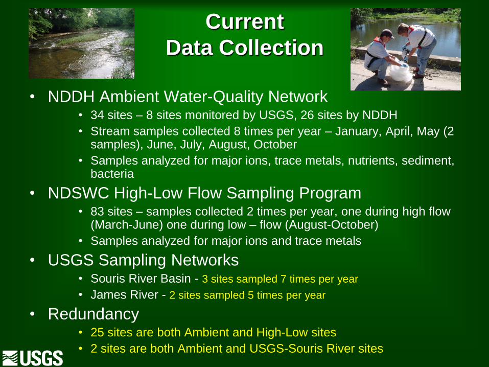
Current
Data Collection
• NDDH Ambient Water-Quality Network • 34 sites – 8 sites monitored by USGS, 26 sites by NDDH
• Stream samples collected 8 times per year – January, April, May (2 samples), June, July, August, October
• Samples analyzed for major ions, trace metals, nutrients, sediment, bacteria
• NDSWC High-Low Flow Sampling Program • 83 sites – samples collected 2 times per year, one during high flow
(March-June) one during low – flow (August-October)
• Samples analyzed for major ions and trace metals
• USGS Sampling Networks • Souris River Basin - 3 sites sampled 7 times per year
• James River - 2 sites sampled 5 times per year
• Redundancy • 25 sites are both Ambient and High-Low sites
• 2 sites are both Ambient and USGS-Souris River sites
Purpose and Scope
1. Provide descriptive statistics and summaries of
water-quality data from sites throughout the
State;
2. Determine trends and loads for selected
constituents and sites with sufficient
concentration and streamflow data;
3. Determine an efficient state-wide network
sampling design for monitoring future water-
quality conditions

Outline
• Analysis methods
• Spatial distribution of concentrations
• Loads and Yields
• Trends
• Sampling design

Analysis Methods
• Examined all data available from 1970-2008 - Data obtained from USGS NWIS database, USEPA STORET database, and electronic files from NDDH
• Trace elements – only used data collected after Jan.1, 1993 because of changes in analytical and field collection methods
• Certain constituents were not evaluated because of large range of laboratory detection limits, highly variable field collection, and variable laboratory analysis methods
• Fecal indicator bacteria, chlorophyll, organic compounds
• Data screening yielded 186 sites across the State with 10 or more samples for most constituents

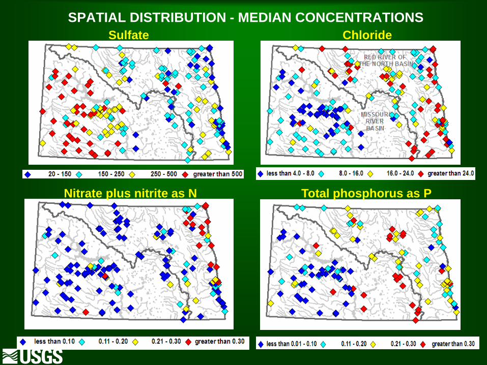
SPATIAL DISTRIBUTION - MEDIAN CONCENTRATIONS
Nitrate plus nitrite as N Total phosphorus as P
Sulfate Chloride
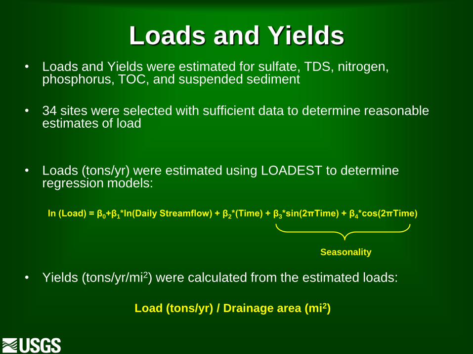
Loads and Yields • Loads and Yields were estimated for sulfate, TDS, nitrogen,
phosphorus, TOC, and suspended sediment
• 34 sites were selected with sufficient data to determine reasonable estimates of load
• Loads (tons/yr) were estimated using LOADEST to determine regression models:
ln (Load) = β0+β1*ln(Daily Streamflow) + β2*(Time) + β3*sin(2πTime) + β4*cos(2πTime)
• Yields (tons/yr/mi2) were calculated from the estimated loads:
Load (tons/yr) / Drainage area (mi2)
Seasonality

Sulfate and TDS Yields

Nutrient Yields

Trends
• Used time series model (QWTREND) to
evaluate flow-related variability and trends
in historical concentrations. Significant
trends were determined using maximum
likelihood estimation and generalized
likelihood ratio tests
• Selected 10 sites with sufficient data

Cannonball River near Breien (site 170)
Year
1975 1980 1985 1990 1995 2000 2005 2010
Heart River near Mandan (site 156)
Wild Rice River near Abercrombie (site 10)
10
100
1000
10000
Knife River at Hazen (site 127)
Red River of the North at Grand Forks (Site 56)
Su
lfa
te c
on
ce
ntr
atio
n,
in lo
ga
rith
m o
f m
illig
ram
s p
er
lite
r
10
100
1000
10000
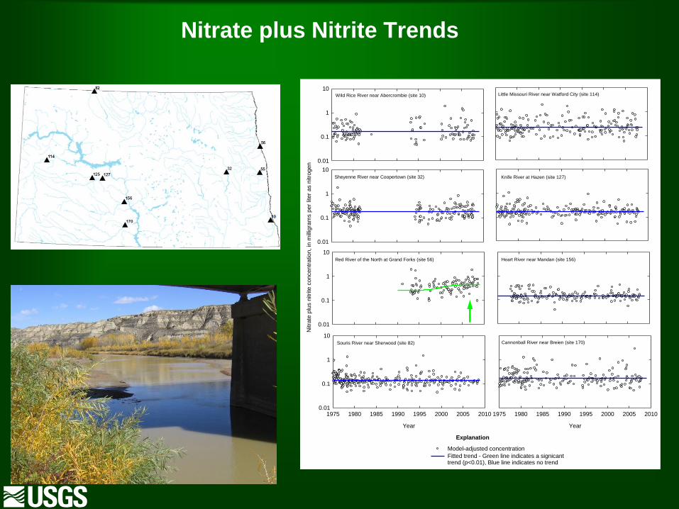
Model-adjusted concentration
Fitted trend - Green line indicates a signicant trend (p<0.01), Blue line indicates no trend
Souris River near Sherwood (site 82)
Year
1975 1980 1985 1990 1995 2000 2005 201010
100
1000
10000
Spring Creek at Zap (site 125)Sheyenne River near Cooperstown (site 32)
10
100
1000
10000
Goose River at Hillsboro (site 55)
10
100
1000
10000
Little Missouri River near Watford City (site 114)
Explanation
Sulfate Trends

Cannonball River near Breien (site 170)
Year
1975 1980 1985 1990 1995 2000 2005 2010
Heart River near Mandan (site 156)
Knife River at Hazen (site 127)
Spring Creek at Zap (site 125)
Souris River near Sherwood (site 82)
Year
1975 1980 1985 1990 1995 2000 2005 2010
To
tal p
ho
sp
horu
s c
on
ce
ntr
atio
n,in
mill
igra
ms p
er
lite
r a
s p
hosp
horu
s
0.001
0.01
0.1
1
10
Model-adjusted concentration
Fitted trend - Green line indicates a signicant trend (p<0.01), Blue line indicates no trend
Little Missouri River near Watford City (site 114)
Explanation
Wild Rice River near Abercrombie (site 10)
0.001
0.01
0.1
1
10
Sheyenne River near Coopertown (site 32)
0.001
0.01
0.1
1
10
Goose River at Hillsboro (site 55)
0.001
0.01
0.1
1
10
Red River of the North at Grand Forks (site 56)
0.001
0.01
0.1
1
10
Total Phosphorus
Trends
Cannonball River near Breien (site 170)
Year
1975 1980 1985 1990 1995 2000 2005 2010
Heart River near Mandan (site 156)
Little Missouri River near Watford City (site 114)
Model-adjusted concentration
Fitted trend - Green line indicates a signicant trend (p<0.01), Blue line indicates no trend
Knife River at Hazen (site 127)Sheyenne River near Coopertown (site 32)
Nitra
te p
lus n
itrite
concentr
ation, in
mill
igra
ms p
er
liter
as n
itro
gen
0.01
0.1
1
10
Souris River near Sherwood (site 82)
Year
1975 1980 1985 1990 1995 2000 2005 20100.01
0.1
1
10
Explanation
Wild Rice River near Abercrombie (site 10)
0.01
0.1
1
10
Red River of the North at Grand Forks (site 56)
0.01
0.1
1
10
Nitrate plus Nitrite Trends

Statewide Sampling Network Design
• When/how often to sample (temporal
design)
• Where to sample (spatial design)
• Look for efficient designs
Highest sensitivity to detect at-site trends for a
given cost (ie, number of samples)
Sites selected to reduce redundancy, hence
maximize information for characterizing
spatial water-quality variability

Temporal Design • Measure sensitivity using characteristic trends
• Definition: the characteristic trend of a design for
a particular season is the size of trend, in
percent per year, that has an 80 percent chance
of being detected after 5 years of sampling
• Seek to minimize the CHTND (ie, maximize
sensitivity) over all seasons and constituents.
• For this analysis, “good” sensitivity was achieved
if all of the CHTND’s were less than 20 percent
for sulfate and TDS and less than 40 percent for
nutrients

1
2
3
4
5
6
7
8
9
10
11
12
13
14
15
16
17
18
19
20
21
22
Knife
River
at Hazen
(site 127)
0 50 100 0 50 100
Cannonball
River near
Brein
(site 170)
Heart
River near
Mandan
(site 156)
0 50 100
0 50 100
Souris River
near
Sherwood
(site 82)
0 100 200
Little
Missouri
River near
Watford City
(site114)
0 50 100
Spring Creek
near Zap
(site 125)
Characteristic trend, in percent per year
Mar
Apr
May
June
July
Aug
Sept
Oct
Nov
Dec
Jan
Feb
Sampled months
De
sig
nn
um
be
r
1
2
3
4
5
6
7
8
9
10
11
12
13
14
15
16
17
18
19
20
21
22
Mar
Apr
May
June
July
Aug
Sept
Oct
Nov
Dec
Jan
Feb
Sampled months
De
sig
nn
um
be
r
0 50 100
Wild Rice
River near
Abercrombie
(site 10)
0 50 100
Sheyenne
River near
Cooperstown
(site 32)
Red River of the
North near
Grand Forks
(site 56)
0 50 1000 50 100
Characteristic trend, in percent per year
Goose River
near
Hillsboro
(site 55)
SAMPLE DESIGN - FREQUENCY TOTAL PHOSPHORUS
1
2
3
4
5
6
7
8
9
10
11
12
13
14
15
16
17
18
19
20
21
22
0 40 80
0 40 80
0 40 800 40 80
0 40 80 0 40 80 0 40 80 0 40 80
1
2
3
4
5
6
7
8
9
10
11
12
13
14
15
16
17
18
19
20
21
22
0 100 200 0 40 80
Wild Rice
River near
Abercrombie
(site 10)
Sheyenne
River near
Cooperstown
(site 32)
Goose River
near
Hillsboro
(site 55)
Red River of the
North near
Grand Forks
(site 56)
Souris River
near
Sherwood
(site 82)
Cannonball
River near
Brein
(site 170)
Heart
River near
Mandan
(site 156)
Knife
River at
Hazen
(site 127)
Little
Missouri
River near
Watford City
(site 114)
Spring Creek
near Zap
(site 125
De
sig
nn
um
be
rD
esig
nn
um
be
r
Mar
Apr
May
June
July
Aug
Sept
Oct
Nov
Dec
Jan
Feb
Mar
Apr
May
June
July
Aug
Sept
Oct
Nov
Dec
Jan
Feb
Sampled months
Sampled months
Characteristic trend, in percent per year
Characteristic trend, in percent per year
SULFATE
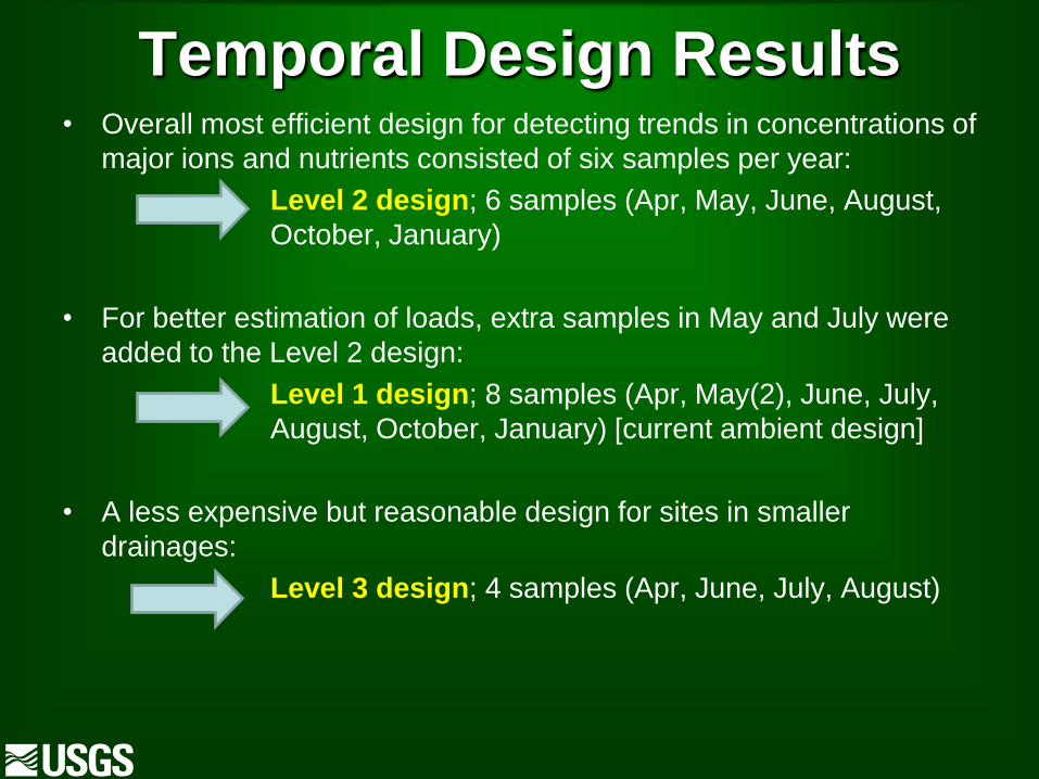
Temporal Design Results • Overall most efficient design for detecting trends in concentrations of
major ions and nutrients consisted of six samples per year:
Level 2 design; 6 samples (Apr, May, June, August,
October, January)
• For better estimation of loads, extra samples in May and July were
added to the Level 2 design:
Level 1 design; 8 samples (Apr, May(2), June, July,
August, October, January) [current ambient design]
• A less expensive but reasonable design for sites in smaller
drainages:
Level 3 design; 4 samples (Apr, June, July, August)
0 10 20 30 40 50 60 70 80 90 1000
20
40
60
80
100
120
140
160
Mean absolute difference between downstream and upstreamflow,as percent of downstream flow
Mea
n a
bso
lute
diff
ere
nce
be
twe
en
dow
nst
ream
and
upst
ream
con
centr
atio
n,
as
perc
ent
of
do
wn
stre
am
co
ncen
tratio
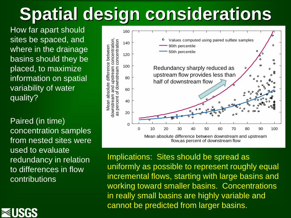
n Values computed using paired sulfate samples
90th percentile
50th percentile
Spatial design considerations How far apart should
sites be spaced, and
where in the drainage
basins should they be
placed, to maximize
information on spatial
variability of water
quality?
Paired (in time)
concentration samples
from nested sites were
used to evaluate
redundancy in relation
to differences in flow
contributions
Redundancy sharply reduced as
upstream flow provides less than
half of downstream flow
Implications: Sites should be spread as
uniformly as possible to represent roughly equal
incremental flows, starting with large basins and
working toward smaller basins. Concentrations
in really small basins are highly variable and
cannot be predicted from larger basins.

Sampling Design – Spatial Network

Total 494
Sample Design summary
Current Sampling networks
Sampling
program
Number
of sites
Sampling
frequency
Total
number of
samples Constituent groups
Ambient 34 8 272 Majors, Trace metals,
Nutrients, bacteria,
sediment
High-Low 81 2 174* Majors, Trace metals
other 6 5-7 32 Majors, Trace metals,
Nutrients,sediment
New sampling network design
Design
level
Number
of sites
Sampling
frequency
Total
number
of
samples
Constituent
groups Objective
1 36 8 288 Majors, Trace
metals, Nutrients,
bacteria, sediment
Trends, Loads
2 17 6 102 Majors, Trace
metals, Nutrients
Fill gaps in trends
network
3 26 4 104 Majors, Trace
metals, Nutrients
Fill gaps in spatial
coverage
Sampling
program
Current Sampling networks
J F M A M J J A S O N D
Ambient X X 2 X X X X
High-
Low X X
other X X X X X X X
Level J F M A M J J A S O N D
1 X X 2 X
X X X
2 X X X X X X
3 X X X X
Total 478

ANY QUESTIONS?


