
Estimating Balance Velocities Using GIS-based Techniques
A Thesis
Presented in Partial Fulfillment of the Requirements for
the Degree Master of Art in the
Graduate School of The Ohio State University
By
Xiaolan Wu, B.S.
* * * * *
The Ohio State University 2002
Master’s Examination Committee:
Approved by: Dr. Alan T. Murray, Adviser Dr. Kenneth C. Jezek _____________________ Dr. Mei- Po Kwan Adviser
Graduate Program in Geography
ii
ABSTRACT
We estimate Antarctic ice flow balance velocities, which are the average speeds
that ice flows through ice cross sections if it is assumed that the input ice of these cross
sections is equal to the output of these cross sections. The balance velocities are
calculated using the OSU Digital Elevation Model (DEM), most recent ice accumulation
rate and ice thickness data for Antarctic. We choose flux algorithms that allow efficient
and accurate computation. The effective merging of digitized flow stripes from satellite
images with our modeled flow directions mitigates the problem of problematic flow
direction estimates in flat areas. In addition standard statistical theory of error
propagation is used to estimate errors for balance velocities from input data measurement
errors. Our new model compares favorably with previous research. Comparison between
balance velocities and flow stripes suggests that fast glacier flow extends deeper into
Antarctica than determined by flow stripe data above.
Key words: Hydrological modeling, Balance velocity, Antarctica

iii
Dedicated to my parents

iv
ACKNOWLEDGMENTS
I would like to express my sincere gratitude to Dr. Kenneth C. Jezek and Dr. Alan
T. Murray for their support and valuable instruction during the two years of my Master ‘s
study. They have helped to shape me as a researcher and a person. Without their patience
and insight I would not have completed my Master’s education successfully.
Dr. Mei-Po Kwan has been very bennefical to me and I am grateful for her
participation as a committee member.
I have enjoyed the chance to work with my colleagues in the Remote Sensing Lab
at the Byrd Polar Research Center. I have worked closely with Hongxing Liu, Zhiyuan
Zhao, Gi-Choul Ann, Kee-Tae Kim, Terresa Van Vleck, Tom Kassebaum, Katy
Noltimier, Leigh Stearns and Jan Wuite. They helped me a lot and pleasantly.
I would also like to express my deepest thanks to my husband for his patience and
support, and my parents for their encouragement and willingness to help out.

v
VITA November, 1978 Born – Jiujiang, Jiangxi P. R. China 1995 –1999 B.S. Geography, Peking University, China 2000 – 2002 Geography, the Ohio State University
Graduate Research Associate in Remote Sensing Lab Byrd Polar Research Center The Ohio State University
FIELD OF STUDY Major Field: Graduate Program in Spatial Analysis Method

vi
TABLE OF CONTENTS Page
ABSTRACT............................................................................................................. ii
DEDICATION......................................................................................................... iii
ACKNOWLEDGEMENTS..................................................................................... iv
VITA........................................................................................................................ v
TABLE OF CONTENTS......................................................................................... vi
LIST OF FIGURES................................................................................................. ix
CHAPTERS
1. INTRODUCTION............................................................................................. 1
2. BALANCE VELOCITY ………...............................................….................... 5
2.1 Introduction...............……......................…….............................. 5
2.2 Previous methods to estimate balance velocity............................ 7
2.3 Review of related methods in hydrology....….............................. 10
2.4 Limitations of previous approaches……...................................... 12
3. FLOW DIRECTION.......................................................................................... 16
3.1 Introduction and previous work.................................................... 16
3.2 Fitting plane algorithm…………….............................................. 18
3.3 Flow stripes digitized from Radarsat Image..….........……….…. 20
3.4 Flow direction from flow stripes……..………………………… 21
3.5 Final flow direction map............................................................... 26
4. FLUX ESTIMATION................……................................................................ 29
4.1 Introduction................................................................................... 29
4.2 Partition schemes.......................................................................... 30
4.3 Flux algorithms ...................…..................................................... 31
4.3.1 Uplsope area calculation (Mark, 1988)…………………. 32
4.3.2 DEMON-Upslope algorithm (Costa-Cabral and Burges, 1994)……………………………………………………..
32
4.3.3 DEMON-Downslope algorithm (Costa-Cabral and Burges, 1994)…………………………………………....
33
4.3.4 Modified Costa-Cabral and Burges algorithm………….. 35
4.3.5 Comparison of flux algorithms…………………….…… 36
4.4 Limitations of flux algorithms.................…......................…....... 37
4.4.1 Diffusion problem………………………………………. 37
4.4.2 Cardinal partitioning scheme problem………………….. 40
4.4.3 Cell-size problem……………………………………….. 41
5. ANTARCTICA ICE SHEET BALANCE VELOCITY....…................…….... 42
5.1 Introduction................................................................................... 42
5.2 Data description............................................................................ 42
5.3 Balance velocity estimation.......................................................... 46

viii
5.3.1 DEM preparation............................................…............... 46
5.3.2 Flow direction estimation..............................…................ 46
5.3.3 Flux estimation..............................................…................ 47
5.3.4 Balance velocity estimation...........................…............... 47
5.4 Error estimation..........................................................….............. 49
5.4.1 Random error from input data.........................….............. 49
5.4.2 Errors in algorithmic calculations .....................…........ 53
5.5 Result validation...............................................................…........ 54
5.5.1 Lamber glacier......................................................…......... 54
5.5.2 East Antarctic ice stream interferometry velocity…......... 58
5.5.3 Flow pattern comparison.......................................…........ 61
6. CONCLUSION................................................................................….............. 63
REFERENCES........................................................................................................ 65
ix
LIST OF FIGURES Figure Page 2.1 Concept of balance velocity…..…………..……………………….……. 7 2.2 Grid cell and its neighbors……………………………………………… 8 2.3 Flux partition……………………………………………………………. 9 2.4 Fitting plane algorithm………………………………………………….. 11 2.5 Two-dimensional partition scheme……………………………………... 11 2.6 Problem of flux model (Costa-Cabral and Burges, 1994)……………… 14 2.7 Problem of flux model (Costa-Cabral and Burges, 1994)……………… 14 3.1 Fitting plane algorithm of Costa-Cabral and Burges…………………… 17 3.2 Fitting plane algorithm of Tarboton…………………………………….. 18 3.3 Hypothetical DEM……………………………………………………… 19 3.4(a) Digitized flow stripes…………………………………………………… 22 3.4(b) Radarsat Image of Antarctica…………………………………………... 23 3.4(c) The accuracy of digitization……………………………………………. 24 3.5 Process of flow stripes direction………………………………………... 24 3.6 Line point coordinate series…………………………………………….. 25 3.7 Grid of flow strip direction……………………………………………... 26 3.8 Final flow direction grid with flow stripes……………………………... 27 3.9 Direction difference between flow stripe directions and directions from
DEM…………………………………………………………………….. 28

x
4.1 Partition schemes (The upper right cell illustrated the Costa-Cabral and
Burges method. The lower left corner illustrated the Budd and Warner method.)…………………………………………………………………
31
4.2 DEMON-Upslope algorithm……………………………………………. 33 4.3(a) Influence matrix (Costa-Cabral and Burges, 1994)…………………….. 34 4.3(b) Calculation of influence matrix (Costa-Cabral and Burges, 1994)…….. 35 4.3(c) New influence matrix…………………………………………………… 36 4.4(a) Hypothetical DEM……………………………………………………… 38 4.4(b) Flux distribution of DEMON’s Downslope area algorithm (Costa-
Cabral and Burges, 1994)………………………………………………. 38
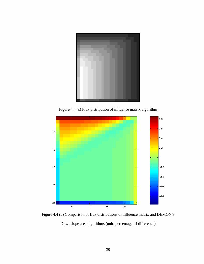
4.4(c) Flux distribution of influence matrix algorithm………………………... 39 4.4(d) Comparison of flux distributions of influence matrix and DEMON’s
Downslope area algorithms (unit: percentage of difference)…………… 39
4.5(a) Conflicts between cardinal partition scheme and process order………... 40 5.1 Hillshade of Antarctica DEM…………………………………………... 43 5.2 Accumulation rate of Antarctica (Vaughan et al. 1999)………………... 44 5.3 Distribution of ice thickness data in BEDMAP compilation (BEDMAP,
2000)……………………………………………………………………. 45
5.4 Ice thickness errors……………………………………………………... 45 5.5 Final surface balance velocity map……………………………………... 49 5.6 Random error of balance velocity using influence matrix algorithm…... 52 5.7(a) Conflict of cardinal partition scheme and front line……………………. 54 5.7(b) Lost ice cells in modified DEMON-Downslope algorithm…………….. 54 5.8 1990/1995 GPS traverse Data…………………………………………... 55
xi
5.9 Comparison between balance velocities and GPS velocities…………… 55 5.10 Flow lines (red line) and GPS measurement points (blue dot)…………. 57 5.11(a) Contributing area……………………………………………………….. 57 5.11(b) Contributing area……………...........................................……………... 57 5.12 Random error of balance velocity profile………………………………. 58 5.13 East Antarctica mosaic overlaid flow stripes and profile lines…………. 59 5.14(a) Profile 1A -- 2A ………………………………………………………….. 59
5.14(b) Profile 1B -- 2B ………………………………………………………….. 60
5.15 Flow stripes (red line) and balance velocity map (gray image)………… 61

1
CHAPTER 1
INTRODUCTION
Polar ice sheets spread and thin under their own weight in a fashion dictated by
the constitutive relationship of ice and the external forces acting on their sides. Under the
simplest of conditions, these processes would result in ice sheets of parabolic surface
profiles and some axial symmetry (Paterson, 1994). Flow through such a simple ice sheet
would be governed by the amount of snow accumulated on the surface and any mass lost
from the base, terminus, or surface melting. In reality, the shape and flow of ice sheets
are much richer features because of the interplay of complex boundary conditions and
even, perhaps, spatial variability in the creep behavior of the ice through crystal
reorientation. This interplay results in a variety of flow styles across both of the polar ice
sheets. These may be characterized by the flow of the interior ice sheet, the surface of
which most closely mimics the predicted near parabolic shape, the flow of ice streams,
which are huge rivers of ice that meander through the interior ice sheet, and the marginal
ice shelves that are vast, nearly flat, slabs of ice floating on the polar ocean.
Ice sheet shape, surface velocity and surface mass balance provide important
clues about ice sheet dynamics and the ice sheet equilibrium state, so acquiring these
2
observations has been the focus of over 50 years of research. Surface shape can be
measured using a variety of altimetric techniques. The shape of the basal interface is
commonly measured with ice sounding radar. Surface accumulation rate is traditionally
measured using in situ methods but several investigations now suggest that remote
sensing techniques may be applicable in some circumstances (Bolzart and Jezek, 2000).
Until very recently, velocity has been measured using in situ data, but feature retracking
on satellite images and radar interferometry are showing that this observation may best be
done from space (Gray et al., 2001).
Given these data, we now pose a question to provide some context for interpreting
the observations. The simplest question is to ask whether or not the ice sheet is in steady
state. That is, we ask whether or not the ice sheet is thickening or thinning. One way to
answer that question is to consider what the physical properties of the ice sheet would
have to be if it were in steady state. A traditional approach has been to take information
on ice sheet surface and basal topography, surface and basal accumulation rate, and
calculate the predicted surface velocity using mass continuity. The calculated velocities
are known as balance velocities because they represent the ice sheet surface speeds that
would result if the amount of snow added annually to the surface equaled the amount of
mass lost from a particular area through advection or melting.
This thesis presents a new approach for computing Antarctic ice sheet balance
velocities. It builds on previous research (Budd and Carter 1971; Budd and Allison 1975;

3
Smith and Budd, 1981; Budd et al. 1982; Radok et al. 1982; Budd and Warner, 1996;
Bamber et al. 2000, 2001) by investigating several new algorithmic approaches and
utilizing the best available data. It also attempts to make use of the recently completed
Radarsat Antarctic Mapping Project SAR mosaic by incorporating derived vector data on
flow direction into balance velocity estimation.
The results of this analysis are compared to measured surface velocities for the
Lambert Drainage Basin and for several of the ice streams which drain into the Filchner
Ice Shelf. The results suggest that only one of the Filchner ice streams may be out of
balance (within the limitations of the data).
The balance velocity results will also be used to constrain velocities that will be
measured using Radarsat interferometric data collected during the Modified Antarctic
Mapping Mission of 2000. The model results will be used in areas of low surface speeds
(less than 20 m per year) and where no other data are available. Because using the
balance velocities biases the interferometric SAR (InSAR) results towards ice sheet
which is in equilibrium, care will be taken to avoid propagating the model results into
regions where non-steady state conditions (such as ice streams) may exist.
The concept of balance velocity is introduced in the second chapter and previous
work on balance velocity and related work in hydrology are reviewed. Major problems
associated with this work are summarized. In the third chapter, previous flow direction
4
algorithms are discussed and a new technique to mitigate flow direction issues in low
slope area is presented. In the fourth chapter, previous flux estimation algorithms are
compared and a modified flux calculation approach is designed which is robust against
DEM errors. In the fifth chapter, Antarctic DEM, accumulation rate and ice thickness
data sets are utilized for the balance velocity calculation. Finally in the sixth chapter,
conclusions are drawn.

5
CHAPTER2
BALANCE VELOCITY
2.1 Introduction
Hydrological models of water flow using DEMs are well known (Peucker and
Douglas, 1975). Essentially, the models compute downslope directions and incorporate
knowledge of water sources to estimate flow patterns and discharge. A similar concept,
balance velocity, has been applied in glaciology (Budd et al. 1971). Balance velocities
are the average speeds of ice flow through ice cross-sections if it is assumed that the ice
input to these cross-sections is equal to the output (Figure 2.1). The following notation is
used:
o
a Accumulation rate with unit of amkg 2/
A Surface area with unit of 2m
iV Balance velocity of input ice with unit of am /
ih Ice thickness of input ice flux gate with unit of m
iw Width of input ice flux gate with unit of m
0V Balance velocity of output ice with unit of am /

6
0h Ice thickness at output flux gate with unit of m
0w Width of output ice flux gate with unit of m
ρ Constant ice density with unit of 3/ mkg
Figure 2.1 shows that there are two sources of ice into the volume element which
is under surface area A: snow accumulated on the surface and ice advected from higher
elevations. The total volume flux of snow from accumulations ( Aao
) equals the
accumulation rate times the surface area. It is assumed that the ice density is constant
(917 3/ mkg ). The advected ice flux ( ρiii whV ) equals the balance velocity of the input to
the volume element times the cross sectional area and the ice density. There is no input
flux to the volume from the sides if the sides are taken parallel to flow lines. The only
discharge of ice from the volume is through the downstream gate and this ( ρ000 whV )
equals the cross sectional area times the balance velocity (to be solved for) and the ice
density. An additional flux (either accumulation or discharge) occurs at the base of the
volume element (melting or freezing), but this possibility is ignored in this analysis.
Since it is assumed that the ice sheet is in equilibrium, the total input ice is equal
to the total discharge.
ρρ 000 whVwhVAa iii =+o
(2.1)
Then the balance velocity (0V ) is:
ρρ
000 wh
whVAaV iii+=
o
(2.2)

7
Figure 2.1 Concept of balance velocity
2.2 Previous Methods to Estimate Balance Velocity
It is easy to understand the concept of balance velocity. However, many
researchers continue to try to design algorithms for estimating balance velocity.
While balance velocity is conceptually easy to understand, algorithms for
efficiently and accurately calculating it involve numerical and / or physical
simplifications. Budd et al. (1971) proposed a flowline-type technique. In their model,
they examined a block of ice bounded by digitized flowlines. Then, the net surface
accumulation was calculated. This amount of ice was considered as the total input ice for
a specific flux gate. Finally, the average balance velocity at this flux gate equaled the
total input ice divided by the flux gate area. This technique was subsequently used by
other researchers (Budd and Carter 1971; Budd and Allison 1975; Smith and Budd, 1981;
Budd et al. 1982; Radok et al. 1982). Although this technique reflects the concept of
balance velocity, its manual processing makes it time consuming to calculate. At places
where flowlines are hard to determine, the result is less accurate than automatic
numerical models designed by others.

8
Budd and Smith (1985) devised an automatic gridded technique that has been
widely used in a number of applications (Budd et al. 1986; Radok et al. 1986, 1987;
Budd and Jenssen 1987, 1989; Mavrakis 1993). In the first step of this technique,
summarized in Budd and Warner (1996), flow direction is calculated by estimating the
direction of steepest slope using a digital elevation model (DEM). In Figure 2.2, cell jix ,
has four cardinal nearest neighbors: jix ,1− , 1, +jix , jix ,1+ and 1, −jix . The surface elevations
for them are denoted jiE , , jiE ,1− , 1, +jiE , jiE ,1+ and 1, −jiE . With this, the horizontal slope
component ( xα ) and the vertical slope component (yα ) for cell jix , are:
xEE jijix ∆−= +− 2/)( ,1,1α (2.3)
yEE jijiy ∆−= +− 2/)( 1,1,α (2.4)
The flow direction (θ ) is given by
ααθ
αα
θ xy == cos,sin (2.5)
Figure 2.2 Grid cell and its neighbors
Next, fluxes are identified for a particular cell. The total ice discharges from cell
jix , are denoted )(,outjiψ ; the inputs of ice to cell jix , from neighboring cells are denoted
1, +jix
jix ,1−
jix ,1+
1, −jix jix ,
9
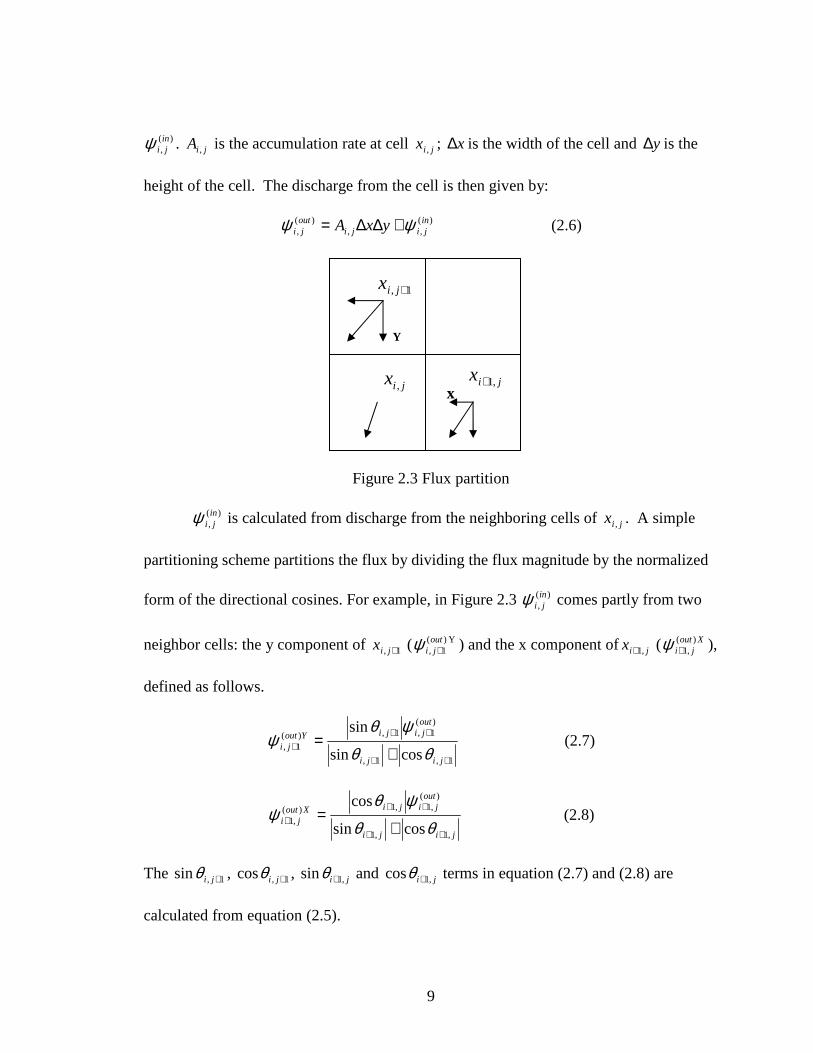
)(,injiψ . jiA , is the accumulation rate at cell jix , ; x∆ is the width of the cell and y∆ is the
height of the cell. The discharge from the cell is then given by:
)(,,
)(,
injiji
outji yxA ψψ +∆∆= (2.6)
Figure 2.3 Flux partition
)(,injiψ is calculated from discharge from the neighboring cells of jix , . A simple
partitioning scheme partitions the flux by dividing the flux magnitude by the normalized
form of the directional cosines. For example, in Figure 2.3 )(,injiψ comes partly from two
neighbor cells: the y component of 1, +jix ( Y )(1,
outji +ψ ) and the x component of jix ,1+ ( Xout
ji)(
,1+ψ ),
defined as follows.
1,1,
)(1,1,)(
1,cossin
sin
++
+++ +
=jiji
outjijiYout
ji θθ
ψθψ (2.7)
jiji
outjijiXout
ji
,1,1
)(,1,1)(
,1cossin
cos
++
+++ +
=θθ
ψθψ (2.8)
The 1,sin +jiθ , 1,cos +jiθ , ji ,1sin +θ and ji ,1cos +θ terms in equation (2.7) and (2.8) are
calculated from equation (2.5).
i,j+1
y
x
Y
jix ,1+
1, +jix
jix ,

10
The calculation is implemented by sorting the cells by descending elevation. From
the highest cell to the lowest cell, the output flux for each cell is calculated so that the
total output flux of every upper input cell is always known from previous calculations.
Implementing this gridded technique, Budd and Warner (1996) created an ice flux
distribution map for Antarctica. Based on this technique, Bamber et al. (2000, 2001)
calculated balance velocity maps for Greenland and Antarctica.
2.3 Review of Related Methods in Hydrology
Previous research on hydrological models provides useful ideas for improving on
balance velocity models. Here several approaches are discussed which have a bearing on
the work conducted as part of this investigation.
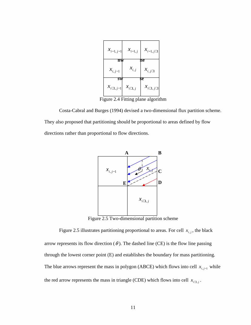
Lea (1992) designed a best fit plane algorithm to get flow direction from a DEM
using the principle of least squares. He fitted a plane to four corners of a cell. The corner
heights are calculated from the average of spot heights of four neighbor cells to each
corner (Figure 2.4). For example,
4,1,,11,1 jijijiji
ne
EEEEC
+++= −−−− (2.9)
“ne”, “nw”, “se”, “sw” represent four corners of center cell jix , . neC , nwC , seC and swC
are the heights at the corners.
11
Figure 2.4 Fitting plane algorithm
Costa-Cabral and Burges (1994) devised a two-dimensional flux partition scheme.
They also proposed that partitioning should be proportional to areas defined by flow
directions rather than proportional to flow directions.
Figure 2.5 Two-dimensional partition scheme
Figure 2.5 illustrates partitioning proportional to areas. For cell jix , , the black
arrow represents its flow direction (θ ). The dashed line (CE) is the flow line passing
through the lowest corner point (E) and establishes the boundary for mass partitioning.
The blue arrows represent the mass in polygon (ABCE) which flows into cell 1, −jix while
the red arrow represents the mass in triangle (CDE) which flows into cell jix ,1+ .
E
jix ,
jix ,1+
1, −jix oθ
i,j
ne nw
se sw
C
D
A B
1, +jix
jix ,1−
jix ,1+
1, −jix jix ,
1,1 +− jix
1,1 ++ jix1,1 −+ jix
1,1 −− jix

12
The fluxes partitioned to cell 1, −jix and to cell jix ,1+ according to the scheme of Costa-
Cabral and Burges (1994) are:
Area of ABCE: 2
12
)90(1
θθ ctgtg−=
−− unit (2.10)
Area of DCE: 22
)90( θθ ctgtg=
− unit (2.11)
Most partitioning schemes lead to a false diffusion of mass. This comes in part
from the partitioning scheme and in part because of the use of Cartesian grids. Costa-
Cabral and Burges (1994) designed a scheme to avoid this problem. The scheme relies
on detailed flow directions to define the contribution area bounded by flow lines (hence
stopping diffusion across flow boundaries). The scheme is complex and Burges (2001)
has pointed out that it is computationally difficult to implement. Moreover, small errors
in flow directions will create significant errors in contribution area, making the model
unstable when implemented over large areas. The model is valuable for simple terrains
and for better understanding the effects of diffusion on conceptually less sophisticated
partitioning algorithms.
2.4 Limitations of previous approaches
Balance velocity calculations begin by estimating the flow direction, taken to be
along the steepest slope. Then, accumulation rate and flow direction are combined in the
model to calculate discharge flux. Dividing the flux by flux-gate area, the balance
velocity is finally specified.

13
All flow direction algorithms require DEM information about neighboring cells.
If the height difference of neighbor cells is small or zero (to the precision of the original
methods and gridding schemes), the algorithms cannot accurately determine the flow
direction for the cell. This problem is particularly acute on polar ice shelves, which are
large floating slabs of ice with typical surface slopes less than o01.0 . Another problem
peculiar to glacier flow is that the ice is assumed to flow down the mean surface gradient.
Superimposed on the mean slope are local variations arising from longitudinal stresses.
Most models deal with longitudinal variations by averaging the surface elevation over a
distance equal to about 10-20 times the ice thickness (Paterson, 1994; Budd and Warner,
1996; Bamber et al. 2001).
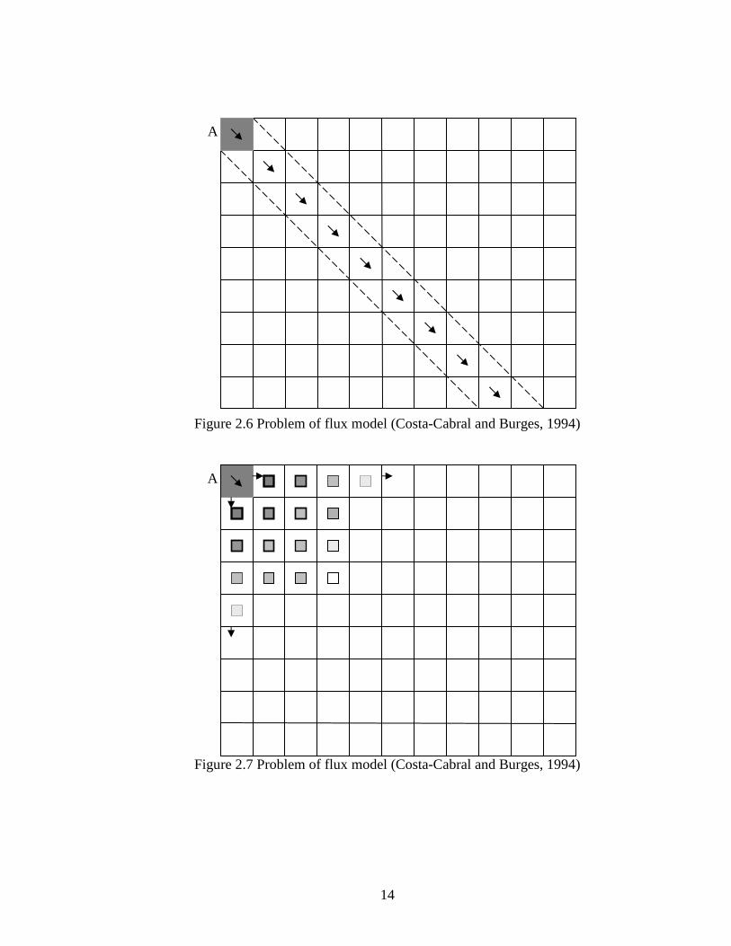
Diffusion is a rarely discussed problem in balance velocity calculations.
Essentially the partitioning schemes allow ice to flow across flow lines. For example,
suppose a planar topography tilting from Northwest to Southeast. Figure 2.6 shows how
the flux at cell A flows to its downstream cells. The region between two dashed lines is
bounded by flow lines. Simple partitioning schemes which allocate ice per the Cartesian
grid diffuse ice outward from this band. In Figure 2.7, the small shaded squares represent
the proportion of the flux from cell A passing into the cells. The diffusion effect is quite
evident.
14
Figure 2.6 Problem of flux model (Costa-Cabral and Burges, 1994)
Figure 2.7 Problem of flux model (Costa-Cabral and Burges, 1994)
A
A

15
Since low slope areas are typical for Antarctica, the problem that flow directions
are affected by DEM errors is important for the Antarctic balance velocity model.
Diffusion distorts flux estimation. Our algorithm, discussed in the following chapters,
attempts where possible to correct some of these limitations. Where not possible, we at
least attempt to quantify the error introduced by the limitations. In Chapter 3, a solution
is proposed which mitigates some of the errors associated with low slope terrain. In
Chapter 4, the degree of diffusion is quantified and discussed.

16
CHAPTER 3
FLOW DIRECTION
3.1 Introduction and previous work
Flow directions are used to map drainage networks as a first step in calculating
mass discharges. Digital elevation models (DEMs) are the basis for deriving flow
directions. There are numerous schemes for estimating flow direction from a DEM. A
simple scheme (D8), assigns eight possible flow directions to each cell (O’Callagham and
Mark, 1984). All of the discharge is assigned to only one flow direction of the eight
possible directions. A refinement is the multiple flow direction model (Quinn et al. 1991;
Freeman, 1991) in which all eight downslope cells are assigned as possible flow
directions (as might be envisioned at the termination of a ridge). Finally fitting plane
algorithms (Lea, 1992; Costa-Cabral and Burges, 1994; Tarboton, 1997) estimate the
direction of maximum slope and assign that direction to be the sole flow direction.
In Chapter 2, Lea’s (1992) fitting plane algorithm was introduced. Costa-Cabral
and Burges (1994) used four diagonal cell heights to fit a plane with a modified version
of Lea’s method and assigned the steepest slope of the plane as the flow direction (Figure
3.1). The x and y components of the slope are:

17
21,11,11,11,1 −+++−−+− −+−
= jijijijix
EEEEα (3.1)
21,11,11,11,1 −+−−+++− −+−
= jijijijiy
EEEEα (3.2)
Figure 3.1 Fitting plane algorithm of Costa-Cabral and Burges
Because only three points are needed to describe a plane, Tarboton (1997) proposed an
algorithm to fit a plane to three cell heights. In Figure 3.2, letter A – H and O are the
center points of the grid cells. The facet OAB is the plane fit to cell heights of jix , , 1, +jix
and jix ,1− . There are eight fitting facets for cell jix , . For facet OAB, the x and y
components of the facing direction of the facet are:
cellsize
EE jijix
1,, +−=α (3.3)
cellsize
EE jijiy
1,11, +−+ −=α (3.4)
Tarboton calculated the facing directions for the eight facets of the cell jix , . Comparing
the steepest slope magnitudes of these eight facets, the facing direction of the biggest
slope facet is assigned as the flow direction for the cell jix , .
i,j
i-1,j-1 i-1,j+1
i+1,j-1 i+1,j+1

18
Figure 3.2 Fitting plane algorithm of Tarboton
The flow direction algorithm used by Budd and others (1996) is similar to the
Costa-Cabral and Burges method but uses the cardinal rather than diagonal points about
the test cell. Referring to Figure 3.2, it fits a plane to the four cells jix ,1− , 1, +jix , jix ,1+ and
1, −jix .
3.2 Fitting plane algorithm
For simple terrain, the above fitting plane algorithms calculate similar flow
directions, but for complicated terrain or DEMs with noisy data, they create different
results. For example, Figure 3.3 is a hypothetical DEM (the numbers in the grid cells are
heights). The flow direction using Lea’s (1992) algorithm is o7.123 , using Costa-Cabral
and Burges (1994) it is o2.199 , using Budd (1996) it is o2.110 , using Tarboton (1997) it
is o3.191 . Essentially the outlier value in the lower center cell biases results which are
8
1 2 3
4
5 6 7
A
B C
D
E
F G
H
O
i-1,j+1 i-1,j
i-1,j-1
i,j-1
i+1,j-1 i+1,j
i+1,j+1
i,j
i,j+1

19
derived from averaging multiple points. The outlier is either ignored or over-emphasized
in schemes which only use diagonal or cardinal points.
Figure 3.3 Hypothetical DEM
When we applied these four algorithms to the Antarctic DEM and compared the
results with flow stripe directions which are the orientation of flow stripes digitized from
image data (detail in next section), we found that the four algorithms behave similarly in
terms of means and deviations of difference from flow stripe directions.
We did not find any conclusive quantitative criteria for selecting one approach
over the other. Ultimately we used the Costa-Cabral and Burges algorithm because the
ice sheet generally exhibits smooth variation, outliers were as best as possible removed in
the original DEM generation, and the fit to the four most widely separated cells (diagonal
cells about the evaluation cell) effectively resulted in additional spatial averaging of the
surface slopes.
3.3 Flow stripes digitized from RAMP Radarsat Image
13
11
14
30
7
9
5.8
12
12

20
The flow-direction distribution map of Antarctica is created by applying the
fitting plane algorithm to the Antarctic DEM. For reasons mentioned above, there are
some flow regimes where the direction is unreliable. Ice streams are relatively narrow
features (order of 50 km) that are difficult to capture with our grid cell spacing (20 km as
discussed later). Ice shelves are very flat and slight errors in the DEM lead to large errors
in calculated flow direction.
The problem of modeling flow in regions of low slope is discussed by Garbrecht
and Martz (1997) who presented an approach that modifies flat surfaces to force the
water to flow from higher to lower terrain. The approach assigns flow directions in flat
areas that force convergence. This approach does not apply to our study because the flow
through ice streams and on ice shelves may be either convergent or divergent. Liang and
Machay (1997, 2000) designed an automated method to assign flow directions for flat
areas using a T-test (difference of means).
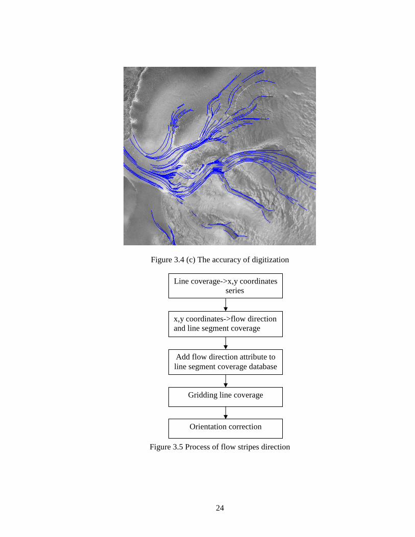
We present an accurate and straight forward method here to mitigate the ice shelf
and ice stream problems. Flow stripes in the fast ice streams and ice shelves are evident
on the RAMP Radarsat imagery (1997). In regions where the ice has been in equilibrium,
these are known to accurately reflect the flow direction. As part of a separate project, the
stripes were manually digitized and converted into Arc/Info line coverage. Figure 3.4(a)
shows the digitized flow stripe map from the Radarsat Image Figure 3.4(b). Figure 3.4(c)
llustrates the accuracy of digitization in east Antarctica.

21
3.4 Flow directions from flow stripes
Our scheme to estimate flow direction from the digitized flow stripes (Sohn and
Jezek, 1997) is as follows.
There are five steps in the process (Figure 3.5). In the first step, the line coverage
of flow stripes is converted to x and y coordinates series. For example (Figure 3.6), line
1l (ABCD) is converted to coordinates series from the starting point to the ending point:
1,4; 3,1; 5,0.5; 7,0.

22
Figure 3.4(a) Digitized flow stripes

23
Figure 3.4(b) Radarsat Image of Antarctica
24
Figure 3.4 (c) The accuracy of digitization
Figure 3.5 Process of flow stripes direction
x,y coordinates->flow direction and line segment coverage
Add flow direction attribute to line segment coverage database
Gridding line coverage
Orientation correction
Line coverage->x,y coordinates series

25
Figure 3.6 Line point coordinate series
Next, the line coverage is separated into line segment coverage. For example, line 1l is
converted into segments AB, BC and CD. Following segmentation from the coordinate
series, the orientation of each line segment of a flow stripe is calculated. For example the
orientation angle for segment AB of line 1l in Figure 3.6 is o7.123 . In the third step, a
new attribute consisting of the facing angle for every segment is added into the line
segment coverage database using Arc/Info. In the fourth step, the line segment coverage
is gridded into a 20km cell-size grid. In the grid, the values of the cells are the facing
angles of the line segments that are nearest to the centers of the cells. In the final step, the
grid value is oriented to reference to the same digitization order because the different
digitization orders of a line, such as digitizing from a starting point to an end or from the
end to the starting point), give different facing angles of the same line segments. Figure
3.7 is the gray grid of flow stripe directions with blue flow stripes overlaid on it.
1l (1,4)
A
(3,1)
B
(5,0.5)
C
(7,0)
D

26
Figure 3.7 Grid of flow strip direction
3.5 Final flow direction map
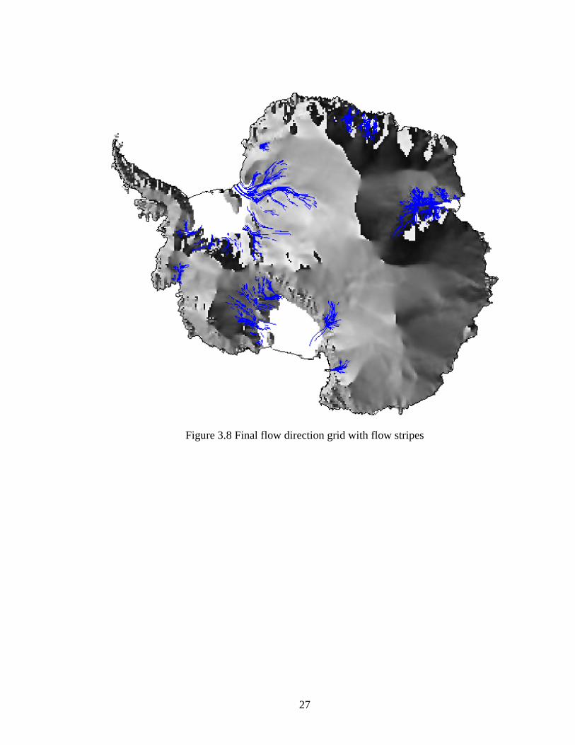
We merge fitting-plane modeled flow-directions from the DEM with the flow
stripe directions by preferentially selecting the flow stripe orientation (Figure 3.8).
Figure 3.9 shows the difference between flow stripe directions and flow directions from
the DEM using a fitting plane algorithm.
We do not calculate flow direction over the flat ice shelves (indicated as white in
Figure 3.8). Very dense flow stripes can be drawn on ice shelves using an enhanced
27
Figure 3.8 Final flow direction grid with flow stripes

28
Figure 3.9 Direction difference between flow stripe directions and directions from DEM
composite Advanced Very High Resolutions radiometer (AVHRR) image (Fahnestock et
al. 2000). In some cases, using the flow stripe directions on ice shelves can improve the
flow direction map (Figure 3.8). However, it has been shown that flow stripes on ice
shelves may be strongly influenced by past changes in ice shelf dynamics. Hence we
choose not to include that information in our analysis.

29
CHAPTER 4
FLUX ESTIMATION
4.1 Introduction
In terms of glacial discharge, flux is the total amount of ice mass passing per unit
time through a cross-sectional area whose surface is perpendicular to the flow direction.
Essentially this represents continuity of mass. If the mass balance of part of the ice sheet
is in equilibrium, then the flux entering a unit volume must equal the flux leaving that
volume. Fluxes are calculated from knowledge about surface accumulation rate and ice
thickness. Flow speeds and directions can be measured, or as done here, balance
velocities can be computed. The magnitude of the balance velocity vector is determined
by mass continuity and the direction of the balance velocity vector is derived from
knowledge about surface elevation as described in the previous chapter.
Ideally, flux is treated as a continuous variable with the property that there is no
flux across stream lines. Practical computation schemes require that the flux calculation
be carried out on a discrete grid that then forces compromises on the analysis. The
compromises arise when the discharge flux from a particular cell is partitioned into
adjacent cells and when the summed discharges are converted into a flux. In this chapter,

30
different partitioning schemes are presented. These are then incorporated into different
flux algorithms for subsequent comparison.
4.2 Partition schemes
Given estimates of flow direction and mass discharge per cell, partition schemes
are used to model how much mass flows from one cell into its neighboring cells. Budd
and Warner (1997) partition the mass by dividing the flux magnitude by the values of
normalized components in directions taken to be aligned with the grid direction. Other
partition schemes distribute the mass according to the magnitudes of slopes or functions
of slopes in the direction of neighboring cells (Quinn et al., 1991; Freeman, 1991). Costa-
Cabral and Burges (1994) proposed a scheme wherein partitioning is proportional to
areas defined by segmenting the cell into two regions separated by the flow direction
vector.
Figure 4.1 is an example illustrating differences between the partitioning schemes
proposed by Budd and Warner (1996) and Costa-Cabral and Burges (1994). oθ is the
flow direction. Suppose the flux at cell jix , is 1 unit. The fluxes partitioned to cell 1, −jix
and to cell jix ,1+ according to the scheme of Budd and Warner (1996) are:
θθθ
θθθ
sincos
sin
)90cos()90sin(
)90cos(
+=
−+−−
unit
θθθ
θθθ
sincos
cos
)90cos()90sin(
)90sin(
+=
−+−−
unit

31
The fluxes partitioned to cell 1, −jix and to cell jix ,1+ according to the scheme of Costa-
Cabral and Burges (1994) are represented by equations 2.10 and 2.11.
Figure 4.1 Partition schemes (The upper right cell illustrates the Costa-Cabral and Burges
method. The lower left corner illustrates the Budd and Warner method.)
4.3 Flux algorithms
Whereas partition schemes model how one cell discharges mass into neighboring
cells, flux algorithms model how all the cell contributions form the drainage system.
Again, different authors have proposed a variety of schemes. For example, Budd and
Warner begin by sorting the DEM from the highest DEM cell to the lowest one to cover
the entire terrain. There are some algorithms that do not require special processing order,
such as the DEMON-downslope algorithm (Costa-Cabral and Burges, 1994), DEMON-
upslope algorithm (Costa-Cabral and Burges, 1994) and upslope area calculation (Mark,
1988). These algorithms are less sensitive to DEM errors by not using DEM order in
processing. Because we introduced the Budd and Warner algorithm in Chapter 2,
DEMON algorithms and others are explained in the following sections.
i,j-1
i+1,j
i,j oθ
A B
C
D E
32
4.3.1 Upslope area calculation (Mark, 1988)
This algorithm is a recursive procedure. First it identifies cells discharging into
the reference cell. If the discharge fluxes of the cells are known, then the flux of the
reference cell is calculated. If the flux from a potential discharge cell is unknown because
the computation has not proceeded far enough along, the calculation proceeds to find the
discharge cells for that new reference cell. The calculation proceeds iteratively until all
of the discharges feeding the original reference cell are determined.
We applied Mark’s algorithm in the flux calculation using Antarctica DEM and
ice accumulation rate and compared the result with Budd and Warner algorithm (1996).
We found that the algorithm overestimates the contributing area by about 20% in many
places, though the shape of the ice stream networks are reasonable. Mark’s algorithm
uses flow directions to trace the contributing areas. The 20km cell-size flow direction
grid cannot define the flow lines very accurately, so small errors in the flow directions
create erroneously bigger contributing areas.
4.3.2 DEMON-Upslope algorithm (Castal-Cabral and Burges, 1994)
This algorithm calculates the contributing areas for every cell by tracing the flow
lines passing through cells which define the boundary of contributing areas. The tracing
stops until the ridges or the terrain boundary are encountered. Then the sums of the mass
accumulated over the contributing area correspond by definition to the fluxes through
every cell. Figure 4.2 shows the contributing areas for cell A with gray shading. The sum
of the mass accumulated over this region is the flux of cell A. There are two major

33
problems with this algorithm. Because it relies on flow directions to define contributing
areas, flow direction errors create large errors in contributing areas. When two flow lines
do not terminate within one cell, it is hard to estimate contributing areas. Thus the
algorithm is difficult to implement in a computer program.
Figure 4.2 DEMON-Upslope algorithm
4.3.3 DEMON-Downslope algorithm (Costa-Cabral and Burges, 1994)
In this algorithm, each cell is treated as an initial condition wherein the flux
entering the cell is simply the surface accumulation rate (advected fluxes are not included
in the flux of the cell chosen for the start of the calculation). The discharge flux from the
initial cell is allowed to flow downslope as an advective term until it encounters cells that
are sinks or leaves the terrain. Once the discharge from every cell is calculated into a so
call influence matrix, the total mass passing through each cell is summed (both
A

34
accumulation and advection terms). In this way, the total mass passing through a
particular cell equals the total mass drained by every upstream cell.
The influence matrix idea is illustrated Figure 4.3(a)). The gray region is the
influence matrix of the cell A. Every cell in the gray region receives advected mass from
cell A in an amount determined by the partitioning scheme. The boundaries of the
influence matrix are flow lines so that there is no diffusion of mass across the boundary.
Figure 4.3(b) is an example of how the value for cell B in the influence matrix is
determined by flow lines. The darker region in cell A is the mass that passes through cell
B. Though the influence matrix determined by flow lines is conceptually very accurate, it
is hard to write an efficient and accurate computer program (Burges, 2001).
Figure 4.3 (a) Influence matrix (Costa-Cabral and Burges, 1994)
A

35
Figure 4.3 (b) Calculation of influence matrix (Costa-Cabral and Burges, 1994)
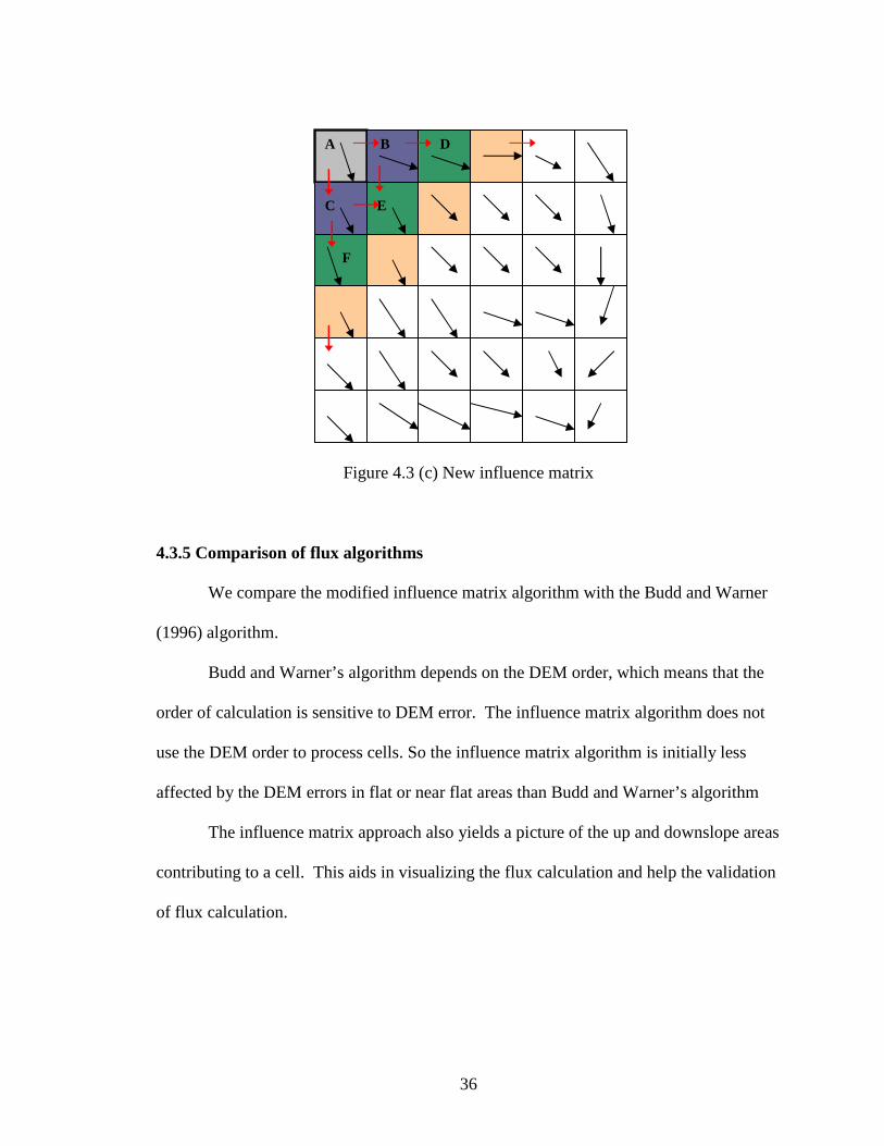
4.3.4 Modified Costa-Cabral and Burges Algorithm
We modify the influence matrix calculation by adopting a simpler partition
scheme. This allows for a tractable code while retaining the advantage that there is no
special ordering of the cells in the calculation. The new algorithm does not build flow
lines. It successively partitions mass from one cell into its downslope cells according to
the partitioning scheme proposed by Costa-Cabral and Burges. Partitioning proceeds until
the edge of the terrain is reached (Figure 4.3(c)). In the Figure, A is partitioned into B and
C. Then B is partitioned into D and E; C is partitioned into E and F. The cells with the
same colors are processed at the same time – we call the ensemble of cells the front line.
Front lines are not determined manually. They arise automatically and somewhat
artificially from the process order. As discussed later, the front lines contribute to the
cardinal partitioning scheme problem discussed later in section 3 in detail.
A
B
36
Figure 4.3 (c) New influence matrix
4.3.5 Comparison of flux algorithms
We compare the modified influence matrix algorithm with the Budd and Warner
(1996) algorithm.
Budd and Warner’s algorithm depends on the DEM order, which means that the
order of calculation is sensitive to DEM error. The influence matrix algorithm does not
use the DEM order to process cells. So the influence matrix algorithm is initially less
affected by the DEM errors in flat or near flat areas than Budd and Warner’s algorithm
The influence matrix approach also yields a picture of the up and downslope areas
contributing to a cell. This aids in visualizing the flux calculation and help the validation
of flux calculation.
A B
C E
F
D

37
Both algorithms suffer from the diffusion problem. They are also sensitive to the
cell size chosen and the manner in which flux is partitioned between cells. In the
following section these problems are discussed in detail.
4.4 Limitations of the flux algorithm
We discuss three limitations of the flux algorithms associated with diffusion, cell
size and partitioning schemes.
4.4.1 Diffusion problem
By diffusion we mean the artificial distribution of mass away from boundaries
that would properly be identified as flow lines. We use a simple hypothetical terrain to
examine the degrees of diffusion for different flux algorithms. Figure 4.4 (a) is the
hypothetical DEM which represents a plane tilting from Northeast to Southwest. The
flow direction from the DEM is o120 from North direction represented by the arrow. The
accumulated mass is assumed to be uniform (10 units). Because DEMON’s Downslope
area algorithm (Costa-Cabral and Burges, 1994) tries to incorporate a flow band
constraint, we use it as a control. The flux modeled by DEMON’s Downslope area
algorithm is shown in Figure 4.4 (b). The flux modeled by our influence matrix algorithm
is shown in Figure 4.4 (c). Figure 4.4 (d) is the percentage difference between the
influence matrix algorithm and the DEMON’s Downslope area algorithm. In Northwest
sector the differences are on average about 40% disregarding the boundary results, which
means the influence matrix algorithm overestimates flux. The error is biased to

38
Northwest direction because the flow direction o120 causes more flux to be partitioned in
the west direction and less flux in the south direction. Budd and Warner’s (1996)
algorithm creates similar results as influence matrix algorithm for the simple terrain.
Figure 4.4 (a) Hypothetical DEM
Figure 4.4 (b) Flux distribution of DEMON’s Downslope area algorithm
(Costa-Cabral and Burges, 1994)
39
Figure 4.4 (c) Flux distribution of influence matrix algorithm
Figure 4.4 (d) Comparison of flux distributions of influence matrix and DEMON’s
Downslope area algorithms (unit: percentage of difference)

40
4.3.2 Cardinal partitioning scheme problem
The partitioning scheme relegates the flux from a cell into its cardinal
downstream cells. For example, figure 4.5(a) is a valley terrain where cell jix , flows to
cell 1,1 +− jix . The numbers in cells are their heights. According to the cardinal point
partitioning schemes, flux from cell jix , is partitioned into cell jix ,1− and cell 1, +jix , but
these are higher than cell jix , . This results in a conflict which causes cell 1,1 +− jix to lose
mass from cell jix , .
Figure 4.5(a) Conflicts between cardinal partition scheme and process order
This kind of conflict effects Budd and Warner’s algorithm when the incorporated
flow stripe derived directions conflict with the maximum slopes derived from the original
DEM. The influence matrix algorithm also has this problem when flow directions are
curved. In Chapter 5, this problem is discussed further.
i,j
i-1,j
(349)
(350) (330)
(360) (350)
(345) i,j+1
(347) i-1,j+1

41
4.3.3 Cell-size problem
The DEM assumes the terrain within a cell is uniform. Smaller scale terrain than
the cell-size cannot be modeled by DEM. Although the DEM has a minimum 200 m cell
size, it is well known that ice flows in the direction of maximum surface slope averaged
over 10 –20 times the ice thickness. This results in a fairly coarse grid. For example,
when we apply the flux algorithm to Antarctica DEM with 20km cell-size, some small
streams such as upper Ice Stream B cannot be detected.

42
CHAPTER 5
ANTARCTICA ICE SHEET BALANCE VELOCITY
5.1 Introduction
In this chapter, we present a new our balance velocity model. We describe the
data and any preprocessing needs. We go on to validate the model by comparing it with
independent estimates of surface velocity. Finally, we compare estimated balance
velocity with Radarsat flow stripes to answer questions about the dynamics of the ice
sheet.
5.2 Data Description
We used four primary data sets in this analysis: the OSU digital elevation model
of Antarctica (Liu et al. 1999); the BEDMAP (2000) basal surface topography model;
surface accumulation rates (Vaughan et al. 1999); and RAMP flow stripes. We describe
these in the following sections.
5.2.1 OSU DEM of Antarctica
43
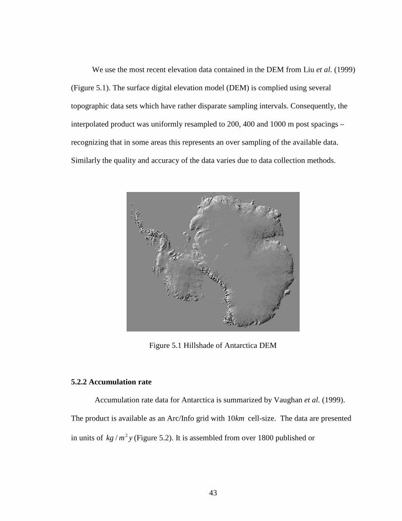
We use the most recent elevation data contained in the DEM from Liu et al. (1999)
(Figure 5.1). The surface digital elevation model (DEM) is complied using several
topographic data sets which have rather disparate sampling intervals. Consequently, the
interpolated product was uniformly resampled to 200, 400 and 1000 m post spacings –
recognizing that in some areas this represents an over sampling of the available data.
Similarly the quality and accuracy of the data varies due to data collection methods.
Figure 5.1 Hillshade of Antarctica DEM
5.2.2 Accumulation rate
Accumulation rate data for Antarctica is summarized by Vaughan et al. (1999).
The product is available as an Arc/Info grid with km10 cell-size. The data are presented
in units of ymkg 2/ (Figure 5.2). It is assembled from over 1800 published or

44
unpublished in situ measurements. The uncertainty of the data is approximately 5%
(Vaughan et al. 1999).
Figure 5.2 Accumulation rate of Antarctica (Vaughan et al. 1999)
5.2.3 Ice Thickness
Ice thickness was compiled as part of the BEDMAP project (Lythe, et al. 2000).
The data is provided in an Arc/Info grid with km5 cell-size. It is based on about 2 million
ice thickness observations by 12 countries over the last five decades (Figure 5.3). The
accuracy of ice thickness is different in different regions and ranges from 10 to 180
meters (Lythe, et al. 2000). A few areas, such as the Amery Ice Shelf, Ronne-Filchner Ice
Shelf and Siple Coast, have good accuracy and excellent coverage (Lythe, et al. 2000).
Other areas, such as large parts of East Antarctica, are covered by 50km spaced flight-
lines or with little to no data at all (there, ice thickness is based on gross interpolation or

45
model results) (Lythe, et al. 2000). We estimated ice thickness errors according to known
properties of the data collection methods (Figure 5.4).
Figure 5.3 Distribution of ice thickness data in BEDMAP compilation (BEDMAP, 2000)
Figure 5.4 Ice thickness errors
46
5.3 Balance Velocity Estimation
This section summarizes the balance velocity estimation, including DEM
preparation, flow direction estimation, flux estimation and balance velocity estimation.
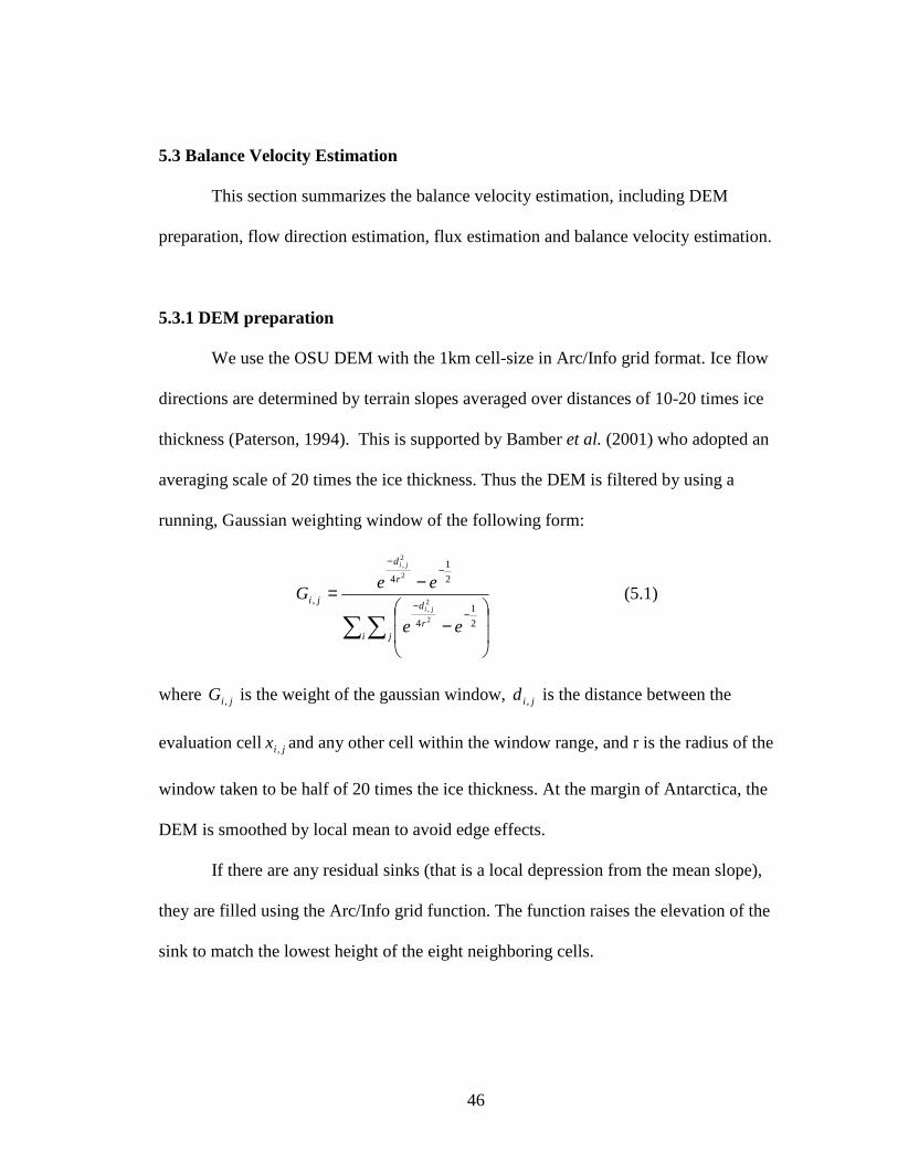
5.3.1 DEM preparation
We use the OSU DEM with the 1km cell-size in Arc/Info grid format. Ice flow
directions are determined by terrain slopes averaged over distances of 10-20 times ice
thickness (Paterson, 1994). This is supported by Bamber et al. (2001) who adopted an
averaging scale of 20 times the ice thickness. Thus the DEM is filtered by using a
running, Gaussian weighting window of the following form:
∑ ∑
−
−=−
−
−−
i jr
d
r
d
ji
ee
eeG
ji
ji
2
1
4
2
1
4
,
2
2,
2
2,
(5.1)
where jiG , is the weight of the gaussian window, jid , is the distance between the
evaluation cell jix , and any other cell within the window range, and r is the radius of the
window taken to be half of 20 times the ice thickness. At the margin of Antarctica, the
DEM is smoothed by local mean to avoid edge effects.
If there are any residual sinks (that is a local depression from the mean slope),
they are filled using the Arc/Info grid function. The function raises the elevation of the
sink to match the lowest height of the eight neighboring cells.
47
The filtered DEM is resampled into a 20km cell-size grid, which corresponds to
the cell size used by Budd and Warner (1996).
5.3.2 Flow direction estimation
As explained in Chapter 3, flow direction is first derived from the DEM using the
Costa-Cabral and Burges fitting plane algorithm. Then, we merge the flow direction grid
with the flow stripe directions by preferentially selecting the flow stripe orientation
(Figure 3.8). Incorporation of vector data mitigates the sensitivity of flow direction to
DEM errors in low slope areas and to some extent, regions of converging flow.
5.3.3 Flux estimation
As discussed in Chapter 4, a modified version of DEMON-Downslope algorithm
provides an efficient and reasonably accurate computational approach. The balance
velocity model is based on this algorithm.
5.3.4 Balance velocity estimation
We calculate the flux for every grid cell. The flux gate area for every grid cell is
the cell-size dimension multiplied by the ice thickness. We treat the flux as a scalar with
a fractional part of the flux going in the x and y directions. The portion of the flux in the
x direction ( xF ) is related to an equivalent balance speed (xV ) as:
WHVF xx ⋅⋅= (5.2)
Where H is the ice thickness, W is the grid cell-size dimension.
48
The portion of the flux in the y direction (yF ) is related to equivalent balance speed (yV )
as:
WHVF yy ⋅⋅= (5.3)
and
yx FFF += (5.4)
In turn, we define the components of the velocity vector (V) as:
WHVWHVF xx ⋅⋅⋅=⋅⋅= θcos (5.5)
WHVWHVF yy ⋅⋅⋅=⋅⋅= θsin (5.6)
Still treating everything as a scalar we add these equations to get:
( )θθ cossin +⋅⋅=
WH
FV (5.7)
where F is the flux for a grid cell with unit of 13 −ym , θ is flow direction previously
determined by steepest slope from DEM.
Because balance velocity (V) is the average velocity at the flux gate, the ice
surface balance velocity (sV ) is set equal to the balance velocity divided by 0.89 (Budd
and Warner 1996). The ratio takes into account the fact that the velocity decreases from
the surface towards the bed.
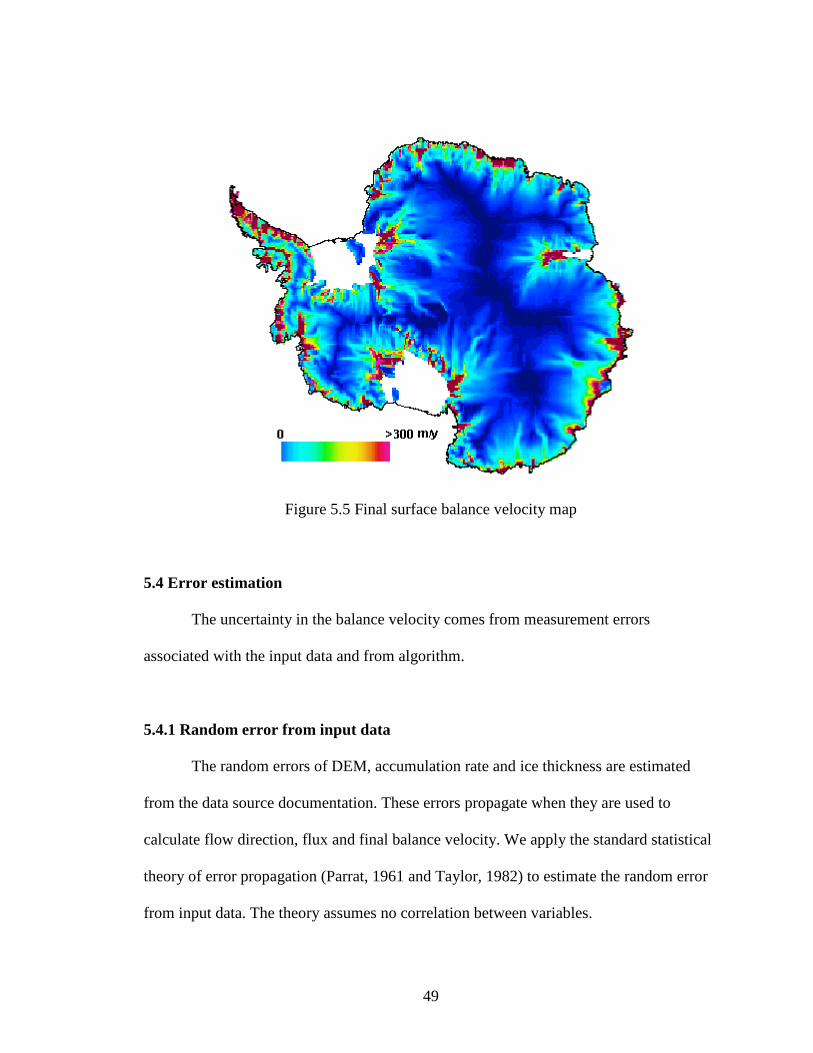
Figure 5.5 is the final surface balance velocity map.
49
Figure 5.5 Final surface balance velocity map
5.4 Error estimation
The uncertainty in the balance velocity comes from measurement errors
associated with the input data and from algorithm.
5.4.1 Random error from input data
The random errors of DEM, accumulation rate and ice thickness are estimated
from the data source documentation. These errors propagate when they are used to
calculate flow direction, flux and final balance velocity. We apply the standard statistical
theory of error propagation (Parrat, 1961 and Taylor, 1982) to estimate the random error
from input data. The theory assumes no correlation between variables.

50
The flow direction is determined by (see Chapter 3):
21,11,11,11,1 −+++−−+− −+−
= jijijijix
EEEEα (5.8)
21,11,11,11,1 −+−−+++− −+−
= jijijijiy
EEEEα (5.9)
)(tan 1
x
y
αα
θ −= (5.10)
So the standard deviation of flow direction (θd ) is:
( ) ( )21,11,1
21,11,1
22
−++−++−− −+−=
jijijiji EEEE
zdd θ (5.11)
dz is the random DEM error between neighbor cells.
Flux is calculated by the modified DEMOM-Downslope algorithm which starts to
calculate the influence matrix for every cell and then sums up the matrixes. For a single
influence matrix of cell ix , the discharge flux of cell ix ( 0,iF ) into the influence matrix is
the accumulation rate (o
A ) of the cell multiplied by the surface area of the cell (S). The
flux of its downcell ( kiF , ) in the influence matrix accumulates input fluxes from its
upcells.
0=j SAFi
o
=0, (5.12)
While ice has downcell, that is, ice does not reach the edge of the Antarctica or
ice does not flow into a sink, if kix , is the downcell, the flux for cell kix , in the influence
matrix of ix ( kiF , ) is given by:
51
0≠= kj 1,1, −= kiki FF λ 2
tan1
θλ = (5.13)
1λ is the partitioning rate from Costa-Cabral and Burges partitioning scheme. Here we
just consider the partition of one cardinal direction. For the partition of the other direction,
the partitioning rate2λ equals:
2
tan12
θλ −= (5.14)
Once influence matrixes for all cells on the Antarctica are completed, they are
added up to get total flux for every cell. The total flux for cell jx ( jF ) is:
jnjjj FFFF ,,1,0 ...+++= (5.15)
where jF ,0 , jF ,1 ,…, jnF , are the fluxes at cell jx in all influence matrixes.
So the standard deviations of fluxes are:
0=j 0
0, AdSdFi ⋅= (5.16)
While ice has downcell, that is, ice does not reach the edge of the Antarctica or
ice does not flow into a sink, if kix , is the downcell, the flux error for cell kix , in the
influence matrix of cell ix ( kidF , ) is given by:
0≠= kj 221,
21,1,
2 ))cos
(()(θ
θλ dFdFFd kikiki −− +=
21
θλ tg= (5.17)
Once influence matrixes for all cells on the Antarctica are completed, the total
flux error for cell jx ( jdF ) is given by:
jnjjj FdFdFdFd ,2
,12
,022 ...+++= (5.18)

52
where jdF ,0 , jdF ,1 ,…, jndF , are the flux errors at cell jx in all influence matrixes.
The balance velocity (V) is:
cellsizeH
FV
⋅+⋅=
)cos(sin θθ (5.19)
So the standard deviation of balance velocity ( )dV is:
( ) 2
2
2
2
2
2
)cos(sin
sincos
)cos(sin)cos(sin
+⋅⋅−⋅+
⋅⋅++
⋅+⋅=
θθθθθ
θθθθ cellsizeH
dF
Hcellsize
FdH
cellsizeH
dFVd
(5.20)
Figure 5.6 is the random error of balance velocity using influence matrix algorithm. The
random error is small. It is about 1% of balance velocity. We apply this error analysis to
the test study area discussed in section 5.5.1.
Figure 5.6 Random error of balance velocity using influence matrix algorithm

53
5.4.2 Errors in algorithmic calculation
It is hard to quantify the errors resulting from algorithms, such as the errors
caused by the diffusion problem, cardinal partitioning scheme and cell-size problem. But
we can at least estimate where the problems may be more or less severe. For the lost ice
problem of cardinal partitioning scheme (also refer to section 4.3.3), we create a map to
visualize where the problem happens (Figure 5.7(b)).
Figure 5.7(a) is an influence matrix of a single cell A. The cells with the same
colors are processed at the same time – we call the ensemble of cells the front line. Front
lines are not determined manually. They arise automatically and somewhat artificially
from the process order. Once a front-line cell is processed, we do not allow ice to flow
backwards into the front line. In this example, the cell B flow direction points Southwest.
According to the cardinal partition scheme, its flux should be partitioned to cell C and D,
but cell C is a processed front line. So the part of flux from B which should flow into cell
C is routed to cell D. This procedure to adjust flux flow distorts the influence matrix to
some degree, but it maintains the total flux. All flow direction arrows in red in Figure
5.7(a) represent adjusted cells. For cell E, its flow direction is in the Northwest, so its flux
should be partitioned to cells F and G, but both cells are in a processed front line. Thus
the amount of flux from cell E is lost. It is called lost ice. Though we tried to flow the
flux from cell E to its neighbor cells which are in the same process line as cell E, in
complex terrain, unrealistic flux distribution was created. The black arrows in Figure
5.7(a) indicate the cells that lose ice. Black dots in figure 5.7(b) are the lost ice cells when
the modified DEMON-Downslope approach is applied on Antarctica.

54
Figure 5.7(a) Conflict of cardinal partition scheme and front line
Figure 5.7(b) Lost ice cells in modified DEMON-Downslope algorithm
5.5 Result validation
We compare the balance velocity result with independently measured velocity to
validate our calculation.
5.5.1 Lambert Glacier
A
B C
D
E F
G

55
Figure 5.8 is the Lambert Glacier mosaic (gray image) showing the location of
1990/1995 GPS traverse data (red dots) collected as part of the Australian National
Antarctic Research Expedition.
Figure 5.8 1990/1995 GPS traverse Data
Figure 5.9 Comparison between balance velocities and GPS velocities

56
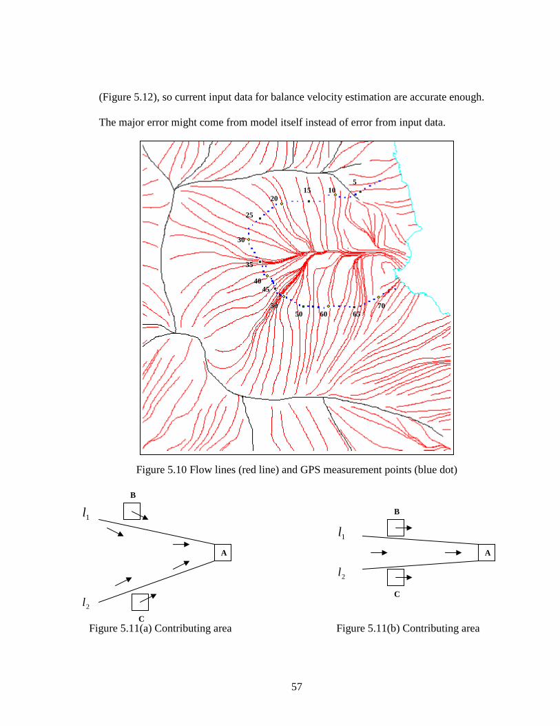
Figure 5.9 shows the GPS velocity profiles, balance velocity implementing the
Budd and Warner algorithm (DEM Sorting) by ourselves (we do not get their codes or
their balance velocities) and balance velocity from the modified DEMON-Downslope
algorithm (Influence matrix) along the traverse line. For the data points from 1 to 10, 15
to 20, 65 to 70, these three estimates are similar which validates the balance velocity
calculation. For data point 13, the balance velocities do not detect the measured velocity
peak, which may simply mean that the feature is too small to be detectable in the 20km
cell-size balance velocities. There are three balance velocity peaks where balance
velocities are obviously higher than GPS measurements, such as data points from 20 to
25, data point 35 and from 40 to 45. Examining the individual contributing areas for these
points, we conclude they are an overestimation by the model rather than disequilibrium of
the ice streams. Figure 5.10 is the flow line map (Liu et al. 1999) derived from the DEM
along with the locations of GPS measurement points. It is clear that those overestimated
velocities are located where flow lines are converging. For those relatively better
estimated velocity points, they are located where flow lines are parallel. We conclude that
the problem occurs where the flow lines are converging. Consequently the contributing
area is likely to be enlarged due to artificial mass diffusion outside of the real flow lines.
This is illustrated in Figure 5.11(a). The lines 1l and 2l are assumed to be real flow lines.
The fluxes of cells B and C flow through cell A because of diffusion. For the parallel
flow lines (Figure 5.11(b)), the contributing area of the cell A is less influenced by the
diffusion of cells B and C which are outside the real flow lines. We draw the profile on
the statistical error (section 5.4). The estimated errors are about 1% of balance velocity
57
(Figure 5.12), so current input data for balance velocity estimation are accurate enough.
The major error might come from model itself instead of error from input data.
Figure 5.10 Flow lines (red line) and GPS measurement points (blue dot)
10 20
30
40
50 60
70
5 15
25
35
45
50 65
1l
2l
A
B
C
1l
2l
B
C
A
Figure 5.11(a) Contributing area Figure 5.11(b) Contributing area

58
Figure 5.12 Random error of balance velocity profile
5.5.2 East Antarctic ice stream interferometry velocity
East Antarctic ice stream interferometric velocities (Zhao and Jezek, 2001) are
based on the SAR interferometric technique, which is widely used to provide high
resolution surface motion vectors. The uncertainty of the flow speed is better than 15
1−ma .
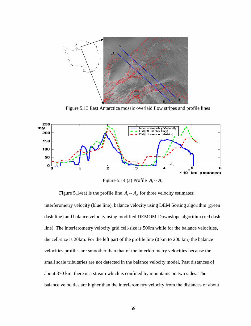
Figure 5.13 is the East Antarctica mosaic (gray image) overlaid with flow stripes
coverage (red line) and profile lines (blue line) used in the comparison of the balance and
interferometric velocities
59
Figure 5.14 (a) Profile 1A -- 2A
Figure 5.14(a) is the profile line 1A -- 2A for three velocity estimates:
interferometry velocity (blue line), balance velocity using DEM Sorting algorithm (green
dash line) and balance velocity using modified DEMOM-Downslope algorithm (red dash
line). The interferometry velocity grid cell-size is 500m while for the balance velocities,
the cell-size is 20km. For the left part of the profile line (0 km to 200 km) the balance
velocities profiles are smoother than that of the interferometry velocities because the
small scale tributaries are not detected in the balance velocity model. Past distances of
about 370 km, there is a stream which is confined by mountains on two sides. The
balance velocities are higher than the interferometry velocity from the distances of about
1A
2A
1B
2B
1A 2A
Figure 5.13 East Antarctica mosaic overlaid flow stripes and profile lines

60
320 to about 370km because the flow directions at the boundary of the stream make ice
flow out of the boundary. There is an obvious offset between influence matrix balance
velocities and interferometry velocity at distances of about 370km. This offset is due to
the low resolution of DEM which causes the boundary between the stream and a nearby
tributary to blur and create an unrealistically wider stream. The DEM Sorting balance
velocities are better at distances of about 370km because ice is constraint not to flow
higher terrain by DEM Sorting algorithm. The elevations at distances from 300km to
370km are higher than those at distances from 370km to 500km so the ice does not flow
out of ice stream in DEM Sorting algorithm. Considering the sum of fluxes across the
gate from distances from about 320km to 500km, influence matrix algorithm sum is more
similar to interferometry velocity than is the DEM Sorting algorithm sum. Also the
balance velocity from DEM sorting algorithm has an unreliable peak at distances 480km,
which might be because the DEM sorting algorithm is more affected by DEM errors than
the influence matrix algorithm.
Figure 5.14 (b) Profile 1B -- 2B
Figure 5.14(b) is the profile 1B -- 2B for the above three velocity estimates. From
0km to 260km, the balance velocities smooth out the small scale tributaries detected by
1B 2B

61
interferometry velocity due the 20km cell-size, but the velocity magnitudes are similar
between balance velocities and interferometry velocity. There is an unreasonable peak at
about 160 km in the model calculated with the DEM sorting algorithm. There an
unrealistic broadening in balance velocity stream from about 260km to 480km as
compared to the interferometry velocity detected stream from 320km to 420km. This is
due to the low resolution DEM from distances about 320km and more. Considering the
sum of fluxes across the gate from distances about 260km to 480km, the sum of balance
velocities is obviously higher than that of interferometry velocity. Mass balance
calculations by Zhao (2001) suggest this area may indeed be slightly out of balance.
5.5.3 Flow pattern comparison
>300
100
200
0
(m/y)
Figure 5.15 Flow stripes (red line) and balance velocity map (gray image)
62
Here the approach is applied to the entire Antarctica. Figure 5.15 is the balance
velocity map from modified DEMON-Downslope algorithm (gray-scale image) overlaid
with RAMP flow stripes (red lines). The whiter color in the gray image indicates higher
velocity; the darker color indicates lower velocity. The flow pattern from the balance
velocity map matches the flow stripes. Though part of the flow stripes are used to force
the ice to flow according to the flow stripes (West Antarctic Ice Streams, ice streams
draining into the Filchner Ice Shelf, Lambert Glacier), the flow pattern of the rest flow
stripes independently matches that from balance velocity. Moreover, balance velocity
extends the ability to look at the flows from ridges. In the lower right area, there are
several obvious ice streams shown by balance velocity but they do not clearly exist in
Radarsat Image. At the very least, this observation deserves scrutiny with interferometric
velocities to see whether the ice sheet is out of balance or whether the flow stripes are not
as reliable indicators of fast glacier flow as thought.
63
CHAPTER 6
CONCLUSION
We have developed a modified flux estimation approach which is robust against
errors in the DEM. Comparisons have been made to existing approaches. The new
approach flexibly incorporates refined flow directions in low slope areas which are
always problematic for traditional flux calculation algorithms because of small DEM
errors. It does not use DEM sorting order to process cells, as does the Budd and Warner
algorithm (1996), which makes our algorithm less sensitive to errors in absolution value
of DEM measures. Our algorithm is easy to implement and allows us to visualize upslope
and downslope areas for an individual cell, which helps to validate results.
We have presented a new technique for incorporating vector information derived
from image data into the flux calculation. This new technique is an easy and straight
forward method which mitigates flow direction problems from DEM errors in flat or near
flat areas.
A new balance velocity model has been structured which compares favorably
with other independently derived surface velocities. Differences between balance velocity

64
and measured velocities may be caused by the diffusion problem. Our study indicates
where diffusion is more or less of a problem.
Comparing Antarctic Mapping Mission (AMM) flow stripes over the Antarctica
with our balance velocity model, in Wilkes Land, we observed agreement in directions
between flow stripes and velocities. However the balance velocity model predicts fast
glacier flow deeper into interior Antarctica. This is an interesting glaciological
observation which will be tested using surface velocity data to be derived from the
Modified Antarctic Mapping Mission interferometry campaign (Jezek, in press).

65
Reference
Bamber, Jonathan L., 1990, Geometric boundary conditions for modeling the velocity field of the Antarctica ice sheet, Annals of Glaciology, Vol. 23. Bamber, J. L., R. J. Hardy, P. Huybrechts and Ian Joughin, 2000, A comparison of balance velocities, measured velocities and thermomechanically modeled velocities for the Greendland ice sheet, Annals of Glaciology, Vol. 30. Bamber, Jonathan L., David G. Vaughan and Ian Joughin, 2000, Widespread complex flow in the interior of the Antarctic ice sheet, Science, Vol. 287. Bamber, J. L., R. J. Hardy and I. Joughin, 2000, An analysis of balance velocities over the Greenland ice sheet and comparison with synthetic aperture radar interferometry, Journal of Glaciology, Vol. 46, No. 152.
Budd, W. F. and D. B. Carter, 1971, An analysis of the relation between the surface and bedrock profiles if ice caps, Journal of Glaciology, Vol. 10, No. 59, 197-209.
Budd, W. F. and I. F. Allison, 1975, An empirical scheme for estimating the dynamics of unmeasured glaciers, International Association of Hydrological Sciences Publication 104 (Symposium at Moscow 1971 – Snow and Ice in Mountainous Areas), 246-256.
Budd, W. F. and I. N. Smith, 1985, The state of balance of the Antarctic ice sheet, Glaciers, ice sheets, and sea level: effect of a 2CO -induces climatic change, report of a Workshop held in Seattle, Washington, September 13 15, 1984, Washington, DC, US Department of Energy, Office of Energy Research, 172-177.
Budd, W. F., D. Jenssen, J. H. I. Leach, I. N. Smith and U. Radok, 1986, The north polar ice cap of Mars as a steady-state systems, Polarforschung, Vol. 56(1-2), 43-63.
Budd, W. F., R. C. Warner, 1996, A computer scheme for rapid calculations of balance-flux distributions, Annals of Glaciology 23. Burges, S. J., 2001, Personal communication.

66
Costa-Cabral, Mariza C. and Stephen J. Burges, 1994, Digital elevation model networks (DEMON): A model of flow over hillshopes for computation of contributing and dispersal areas, Water Resources Research, Vol. 30, No. 6, 1681-1692, 1994. Fahnestock et al. 2000, A millennium of variable ice flow recorded by the Ross Ice Shelf, Antarctica, Journal of Glaciology, Vol. 46, No. 155, 652-664. Freeman, T. G., calculating catchment area with divergent flow based on a reular grid, 1991, Comput. Geoschi., Vol. 7(3), 413-422. Garbrecht, Jurgen and Lawrence W. Martz, 1997, The assignment of drainage direction over flat surfaces in raster digital elevation models, Journal of Hydrology, Vol. 193, 204-213. Jenson, S. K. and J. O. Domingue, 1988, Extracting topographic structure from digital elevation data for geographic information system analysis, Photogrammetric Engineering and Remote Sensing, Vol, 54., No. 11, 1593-1600. Jezek, Kenneth C., 1999, Glaciological properties of the Antarctic ice sheet from RADARSAT-1 synthetic aperture radar imagery, Annals of Glaciology, Vol. 29, 286-290. Joughin, Ian, Mark Fahnestock and Ron Kwok, 1997, Balance velocities of the Green land ice sheet, Geophysical Research Letters, Vol. 24, No. 23, 3045-3048. Lea, Nicholas J., 1993, An aspect-drien kinematic routing algorithm, Overland flow: hydraulics and erosion mechanics, Parsons and Abrahams, 393-408. Liang, Chaojun and D. Scott Mackay, 1997, Feature-based optimization of flow directions and upslope areas on grid-based digital elevation models, In Proceedings of GIS/LIS’97 (Bethesda, MD: American Society for Photogrammetry and Remote Sensing), 45-52. Liang, Chaojun and D. Scott Mackay, 2000, A general model of watershed extraction and representation using globally optimal flow paths and up-slope contributing areas, International Journal of Geographical Information Science, Vol. 14, No. 4, 337-358. Liu, Hongxing, Kenneth C. Jezek and Biyan Li, 1999, Development of an Antarctic digital elevation model by integrating cartographic and remotely sensed data: A geographic information system based approach, Journal of Geophysical Research, Vol. 104, No. B10, 23,199-23,213.
Lythe, Matthew B., David G. Vaughan and BEDMAP Consortium, 2000, BEDMAP: a new ice thickness and subglacier topographic model of Antarctica, in press.

67
Marks, Danny, Jeff Dozier, and James Frew, 1984, Automated basin delineation from digital elevation data, Geo-Processing, Vol. 2, 299-311. Mackay, D. Scott, 1998, Extraction and representation of nested catchment areas from digital elevation models in lake-dominated topography, Water Resource Research, Vol. 34, No. 4, 897-901. O’Callaghan, John F., 1984, The extraction of drainage networks from digital elevation data, Computer vision, graphics, and image processing, Vol. 28, 323-344. Paterson, W. S. B., 1994, The physics of glaciers. Third edition. Oxford.
Quinn, P., K. Beven, P. Chevalier, and O. Planchon, 1991, The prediction of hillslope flow paths for distributed hydrological modeling using digital terrain models, Hydrological Processes, Vol. 5, 59-79
Peucker, T. K. and D. H. Douglas, 1975, Detection of surface-specific points by local parallel processing of discrete terrain elevation data, Computer Graphics and Image Processing, Vol. 4, 375-387.
Radok, U., R. G. barry, D. Jenssen, r. A. Keen, G. N. Kiladis and B. McInnes, 1982, Climatic and physical characteristics of the Greenland ice sheet, Part I and II, Boulder, CO, University of Colorado, Cooperative Institute for Research in Environmental Sciences.
Smith, I. N. and W. F. Budd, 1981, The derivation of past climate changes from observed changes of glaciers, International Association of Hydrological Sciences Publication 131 (Symposium at Canberra 1979 – Sea Level, Ice and Climatic Change), 31-52.
Tarboton, David G., 1997, A new method for the determination of flow directions and upslope areas in grid digital elevation models, Water Resources Research, Vol. 33, No. 2, 309-319.
Vaughan, D.G., J.L. Bamber, M. Giovinetto, J. Russell, and A.P.R. Cooper, 1999, Reassessment of Net Surface Mass Balance in Antarctica, J. Climate, 12, 933-946.
Zhao, Zhiyuan, 2001, Surface velocities of the east Antarctic ice streams from Radarsat-1 interferometric synthetic aperture radar data, Dissertation, the Ohio State University.

68


![Bilayer Segmentation of Live Video · 2018-01-04 · Frequently, motion-based segmentation has been achieved by estimating optical flow ( i.e. pixel velocities) [3] and then grouping](https://cdn.vdocuments.us/doc/165x107/5f371eb038a241102437cd2b/bilayer-segmentation-of-live-video-2018-01-04-frequently-motion-based-segmentation.jpg)


