
Enhanced Monitoring Plans – A Maryland Perspective
David Krask – Air Monitoring ProgramManager
National Ambient Air Monitoring ConferenceSt. Louis, MO
August 10, 2016

Topics Covered
• What constitutes enhanced monitoring? • Why would you want to do it? • Maryland’s ozone challenges. • Examples of Maryland’s enhanced
monitoring. • Costs. • Enhanced Monitoring Plans (EMP)
preparation, submittal and approval process.

What Is Enhanced Monitoring?
From 40CFR Part 58, Appendix D, 5.(h) • Additional ozone monitors beyond
the minimum requirements. • Additional NOx or NOy monitors
above minimum requirements. • Additional VOC measurements
beyond minimum requirements. • Upper air measurements
of meteorology or air pollution concentrations.

Why Would You Want To Do It?
• Surface based monitoring alone cannot determine the nature and origin of your particular ozone problem.
• To produce policy relevant science that will aid in the development and tracking of effective control strategies.
• Evaluate model performance (CMAQ & CAMx), identify weaknesses or areas needing improvements.
• Assist in ozone forecasting. • EPA requires you to.

MARYLAND’S OZONE CHALLENGES

Maryland’s Ozone Challenges

Maryland’s Ozone Challenges

Maryland’s Ozone Challenges The Nocturnal Low Level Jet (NLLJ)
Winds ~ 1000 Feet Above Surface
MDE
Fast-moving, narrow “river” of airtypically around 1000 feet above the surface
In the Mid-Atlantic, typically observedduring the night between Appalachiansand the Atlantic Ocean. Wind speeds can reach 40 mph or
more. Stretches from NC to MD to NJ and
further up the east coast. Seen during most, Mid-Atlantic summer
time air pollution events. Some form of NLLJ on many Code
Orange or Red days Past findings indicate:
Presence of a NLLJ increased Baltimore maximum ozone by 7 ppb.
Ozone concentrations of 90 – 100 ppb have been measured in theNLLJ.

Maryland’s Enhanced Monitoring Examples
Approaches Utilized • Continuous
• Mountaintop monitoring • Radar Wind Profilers (RWPs)
• Seasonal/Episodic • Ozonesondes • LIDAR- Aerosol & Ozone
• Aircraft • Portable Ozone Monitor (POM)
for Land/Water Interface • Short-term Intensive Studies
• Once in a blue moon

Mountaintop Monitoring
3 monitors along Appalachian mountain range can sometimescapture nighttime pollution above the surface. Shenandoah: 1073 m (3,520 ft) Piney Run : 776 m (2,546 ft) Methodist Hill: 676 m (2,218 ft)

Mountaintop Monitoring

Progress at Mountaintop Monitors
Pre and post NOx SIP call benefits at Shenandoah and Methodist Hill.
Diurnal profiles made using May – September hourly ozone data.

Upper-Air Radar Wind Profilers
Horn Point
Piney Run
HU-Beltsville

Hei
ght (
ft)
Beltsville, MD on August 9 - 10, 2010
30 mph for 7 hours is about 210 miles
What does this graph tell us?- Wind direction - Wind speed- From the ground up
August 9th, 11 PM – 7 AM Winds from the southwest at about 25 - 30 mph
August 10th, 10 PM – 8 AM Winds from the southwest at about 25 40 mph
Nocturnal Inversion up to 1000 ft
RWP’s-Measuring the NLLJ Wind Speed and Wind Direction
p. 14

RWP’s-How Big is the NLLJ? May 26 & 27, 2016
Sources: NASA, NOAA MADIS p. 15
Beltsville, MD
New Brunswick, NJ
Stow, MA
Charlotte, NC
8 PM 11 PM 2 AM 5 AM 8 AM 11 AM
NLLJ
Wind Speed and Wind Direction
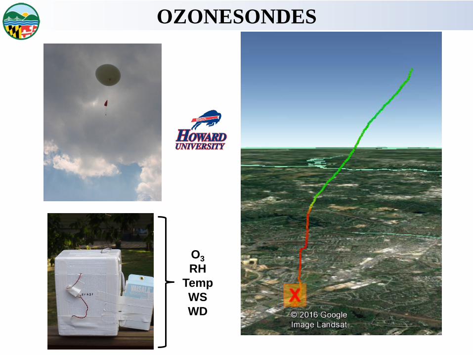
OZONESONDES
O3
RH Temp WS WD
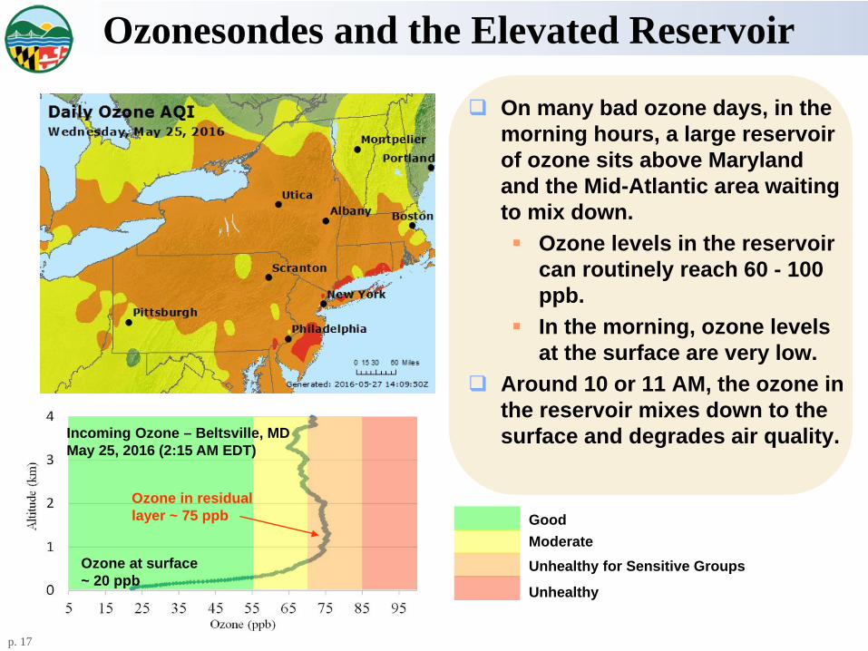
Ozonesondes and the Elevated Reservoir
On many bad ozone days, in the morning hours, a large reservoir of ozone sits above Maryland and the Mid-Atlantic area waiting to mix down. Ozone levels in the reservoir
can routinely reach 60 - 100 ppb.
In the morning, ozone levels at the surface are very low.
Around 10 or 11 AM, the ozone in the reservoir mixes down to the surface and degrades air quality.
Good Moderate Unhealthy for Sensitive Groups
Unhealthy
p. 17
Incoming Ozone – Beltsville, MD May 25, 2016 (2:15 AM EDT)
Ozone at surface ~ 20 ppb
Ozone in residual layer ~ 75 ppb

Measuring Ozone Transport in the NLLJ Howard University launched 2 morning ozonesondes on June 19 - 20, 2012 to
June 19 | June 20, 2012
Mid
nigh
t(E
DT
)
2:30 AM
Ozone Aloft in NLLJ
6:00 AM
High Ozone Aloft NLLJ
20+ mph for 10+ hours Airmass traveled 200+ miles
measure ozone within the Nocturnal Low Level Jet (NLLJ), as captured by MDE’s upper-air radar wind profiler.
p. 18

AEROSOL LIDAR
Baltimore Downtown
Clouds
Aerosols Telescope

UMBC LIDAR •Smoke descended from 3km in height to the surface, as evident by higher fine particle counts and lidar observations, by June 10, 2015
•Smoke plume initially heaviest around and south of DC metro (red sunsets publicized)
•Surface winds on Thursday, June 11, 2015, blew DC polluted air back along I-95 Smoke at the surface
Smoke
LIDAR images courtesy Dr. Ruben Delgado, UMBC
Smoke descended 3000m to reach the surface

TROPOSPHERIC OZONE LIDAR

a
WIND PROFILER – Beltsville, MD b
42
4
4
12
10
8 6
6
Beltsville surface O3 (bottom)
noise, clouds, smoke
Very clean air at 2km above the Nocturnal LLJ
Residual layer of ~80ppb at 1km.
Courtesy of Dr. John Sullivan NASA GFSC

Surface Measurements-VOCs
0.00
10.00
20.00
30.00
40.00
50.00
60.00
70.00 Sum PAMS Target NMHCSpecies
6/9/2015 6/10/2015 6/11/2015 6/12/2015

More Surface Measurements
Hourly PM2.5 data from all Maryland monitors
1) Black Carbon reached peak on June 11 a. Black Carbon is a smoke indicator – highest BC with
highest ozone! 2) “Delta-C” is a proxy wood smoke indicator – reached peak
on June 11 3) Delta-C goes to zero morning of June 12 but quickly rises
after sunrise (same as ozone) – mixing from residual layer?? 4) Dramatic drop off in Black Carbon coincident with ozone
decrease on June 12, in the middle of a 90°F day!!!
2)
1) 3) 4)

AIRCRAFT UMD Cessna 402B Research Aircraft
Aerosol Inlet Gas Inlet
Met Sensors
GPS Position (Lat, Long, Altitude, Speed) Met (T, RH, P, wind speed/direction) Trace gases:
O3: UV Absorption, TECO SO2: Pulsed Fluorescence, modified TECO NO2: Cavity Ring Down, Los Gatos CH4/CO2/CO/H2O: Cavity Ring Down, Picarro K30 CO2 small sensor VOCs: canister samples and GC-FID analysis
Aerosol Optical Properties: Scattering: bscat (@450, 550, 700 nm),
Nephelometer Absorption: bap (565 nm), PSAP Black Carbon: Aethalometer (7-wavelengths)
Data Acquisition: 1 sec
Courtesy: Xinrong Ren, UMD

Aircraft Profiles-Westerly Transport Fingerprint
What does the data tell us about its origin?
High Aloft Ozone 9,000 9,000 9,000 ~ 100 ppb Does not correlate well with CO Correlates well with SO2 3000 - 6000 ft * Not Cars * * Likely Power Plants *
Hei
ght (
ft)
Hei
ght (
ft)
Hei
ght (
ft)
Hei
ght (
ft)
6,000 6,000 6,000
3,000
0 0 20 40 60 80 100 120
Ozone (ppb)
9,000
Correlates with “Aged NOx” * It’s Old *
6,000
3,000
0 2 4 6 8
3,000 3,000
0 0 100 200 300 400 500 600
CO (ppb)
Vertical Profiles of Ozone, CO, SO2 , and NOyat Luray, VA July 15, 1995 at 7 AM
10
0 0 2 4 6 8
SO2 (ppb)
Back Trajectory
NOy (ppb) Data Source: UMD
p. 26
0

Hei
ght (
ft)
Hei
ght (
ft)
Aircraft Profiles-Westerly Transport Fingerprint What does the data tell us about its origin?
3,000
6,000
9,000
3,000
6,000
9,000
3,000
6,000
9,000
Hei
ght (
ft)
Does not correlate well with CO * Not Cars *
Correlates well with SO2 * Likely Power Plants *
High Aloft Ozone ~ 80 ppb 3500 - 5000 ft
0 0 0 0 20 40 60 80 100 120 0 100 200 300 400 500 600 0 2 4 6 8
Ozone (ppb) CO (ppb) SO2 (ppb)
Vertical Profiles of Ozone, CO, and SO2 at Luray, VA July 21, 2011 at 11 AM
Back Trajectory
Data Source: UMD

Comparison of Obs & Modeling
Courtesy of University of Maryland College Park – Russ Dickerson

Flight Plan for Summer 2016 • A morning flight to the west (upwind): spirals at Luray, Winchester, and Cumberland . • An afternoon flight to the west (downwind): spirals over Harford County, MD1 and MD18. • En route vertical profiles between spiral locations to capture vertical gradients. • Missed approaches (low approaches) at regional airports.
Luray
Winchester
Cumberland Harford Airport
MD18
MD1
Courtesy: Xinrong Ren, UMD
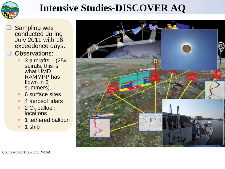
Intensive Studies-DISCOVER AQ
Sampling wasconducted duringJuly 2011 with 16exceedence days.
Observations: 3 aircrafts – (254
spirals, this iswhat UMD RAMMPP has flown in 6 summers).
6 surface sites 4 aerosol lidars 2 O3 balloon
locations 1 tethered balloon 1 ship
Courtesy: Jim Crawford, NASA

DISCOVER-AQ Significant Findings
• Lifetime of alkyl nitrates is much shorter than assumed in the model chemistry module (CB06). Has major implications for ozone production efficiency
• Measured ratio of NOx/CO indicates that the NOx emissions inventory is overestimated by a factor of 2.

POM-Land Water Interface
SCOPE OF PROJECT: Deploy a portable ozone monitor in the Hart Miller Island to investigate the magnitude of ozone concentrations over the Chesapeake Bay.
Hart Miller Island Project

POM-Land Water Interface
MOTIVATION: air quality forecast models have a high bias (that is, forecast too much ozone) over the Bay than what is observed by neighboring shoreline ozone monitors
MAIN QUESTION: What is the magnitude of ozone over the Chesapeake Bay and the interaction between meteorology and ozone along the land/water interface of the Bay?
Forecast 8-hour ozone (background fill (AQI) ) for Maryland on July 11, 2015 overlaid with ozone AQI at ozone monitoring stations across the region (circles).
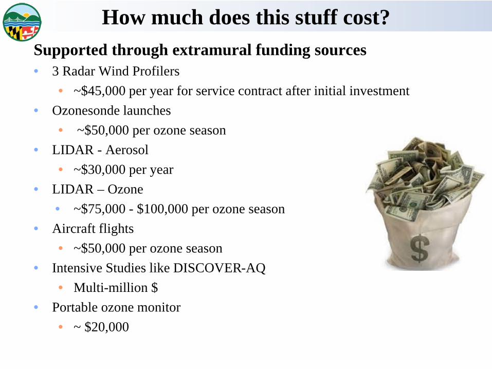
How much does this stuff cost?
Supported through extramural funding sources • 3 Radar Wind Profilers
• ~$45,000 per year for service contract after initial investment • Ozonesonde launches
• ~$50,000 per ozone season • LIDAR - Aerosol
• ~$30,000 per year • LIDAR – Ozone
• ~$75,000 - $100,000 per ozone season • Aircraft flights
• ~$50,000 per ozone season • Intensive Studies like DISCOVER-AQ
• Multi-million $ • Portable ozone monitor
• ~ $20,000

EMP Prep/Submittal/Approval Process
• Stay tuned for more detailed guidance from EPA
• Due Oct. 1, 2019, or 2 years after moderate or above designation
• Will be reassessed and approved as part of 5-year network assessments
• Need to get started very soon

Acknowlegements Michael Woodman-MDE
Daniel Orozco-MDE
Joel Dreesen-MDE
University of Maryland
University of Maryland Baltimore County
Howard University


