
EMAIL SPAM DETECTION USING MACHINE LEARNINGLydia Song, Lauren Steimle, Xiaoxiao Xu
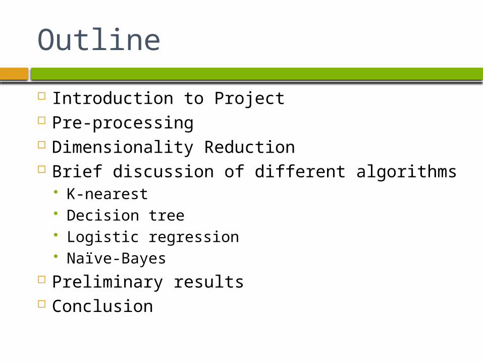
Outline
Introduction to Project Pre-processing Dimensionality Reduction Brief discussion of different algorithms
K-nearest Decision tree Logistic regression Naïve-Bayes
Preliminary results Conclusion

Spam Statistics
Percentage of Spam Emails in email traffic averaged 69.9% in February 2014
Source: https://www.securelist.com/en/analysis/204792328/Spam_report_February_2014
Perc
en
tage o
f sp
am
in
em
ail
traffi
c
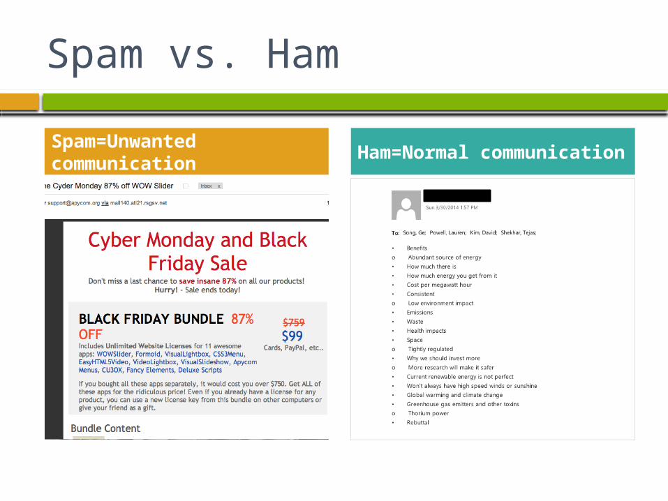
Spam vs. Ham
Spam=Unwanted communication
Ham=Normal communication

Pre-processing
Example of Spam EmailCorresponding File in Data Set

Pre-processing
1. Remove meaningless words2. Create a “bag of words” used in data
set3. Combine similar words4. Create a feature matrix
Email 1Email 2
Email m
“hist
or
y”“s
ervic
e”Bag of Words
history
last
…
service
“last
”

Pre-processing Example
Your history shows that your last order is ready for refilling.
Thank you,
Sam McfarlandCustomer Services
tokens= [‘your’, ‘history’,
‘shows’, ‘that’, ‘your’, ‘last’,
‘order’, ‘is’, ‘ready’, ‘for’,
‘refilling’, ‘thank’, ‘you’,
‘sam’, ‘mcfarland’,
‘customer services’]
filtered_words=[ 'history',
'last', 'order', 'ready',
'refilling', 'thank', 'sam',
'mcfarland', 'customer',
'services']
bag of words=['history',
'last', 'order', 'ready', 'refill',
'thank', 'sam', 'mcfarland',
'custom', 'service']
Email 1Email 2
Email m
“hist
or
i”“s
ervi”
“last
”Bag of Words
histori
last
…
servi
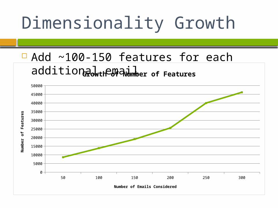
Dimensionality Growth
Add ~100-150 features for each additional email
50 100 150 200 250 3000
5000
10000
15000
20000
25000
30000
35000
40000
45000
50000
Growth of Number of Features
Number of Emails Considered
Num
ber
of
Featu
res

Dimensionality Reduction
Add a requirement that words must appear in x% of all emails to be considered a feature
50 100 150 200 250 3000
100
200
300
400
500
600
Growth of Features with Cutoff Requirement
5%10%15%20%
Number of Emails Considered
Num
ber
of
Featu
res
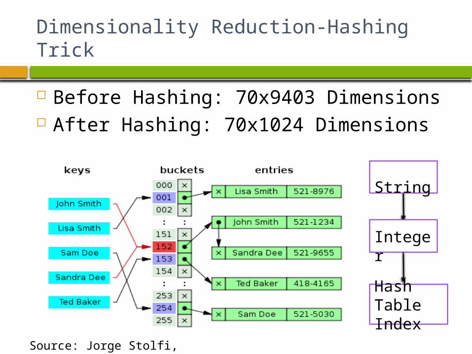
Dimensionality Reduction-Hashing Trick
Before Hashing: 70x9403 Dimensions After Hashing: 70x1024 Dimensions
String
Integer
Hash Table Index
Source: Jorge Stolfi, http://en.wikipedia.org/wiki/File:Hash_table_5_0_1_1_1_1_1_LL.svg#filelinks

Outline
Introduction to Project Pre-processing Dimensionality Reduction Brief discussion of different algorithms
K-nearest Decision tree Logistic regression Naïve-Bayes
Preliminary results Conclusion

K-Nearest Neighbors
Goal: Classify an unknown training sample into one of C classes
Idea: To determine the label of an unknown sample (x), look at x’s k-nearest neighbors
Image from MIT Opencourseware

Decision Tree
Convert training data into a tree structure Root node: the first
decision node
Decision node: if–then
decision based on
features of training
sample
Leaf Node: contains a
class label Image from MIT Opencourseware
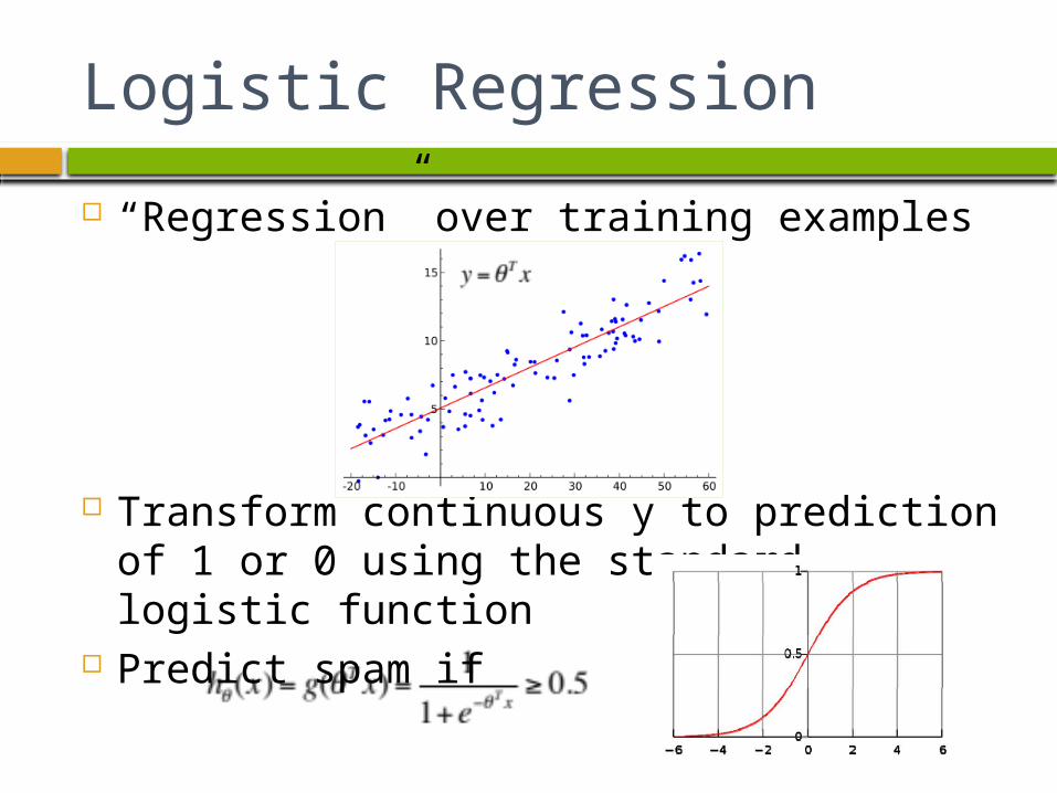
Logistic Regression
“Regression” over training examples
Transform continuous y to prediction of 1 or 0 using the standard logistic function
Predict spam if

Naïve Bayes
Use Bayes Theorem: Hypothesis (H): spam or not spam Event (e): word occurs For example, the probability an email is
spam when the word “free” is in the email
“Naïve”: assume the feature values are independent of each other
Outline
Introduction to Project Pre-processing Dimensionality Reduction Brief discussion of different algorithms
K-nearest Decision tree Logistic regression Naïve-Bayes
Preliminary results Conclusion

Preliminary Results
250 emails in training set, 50 in testing set Use 15% as the “percentage of emails” cutoff Performance measures:
Accuracy: % of predictions that were correct Recall: % of spam emails that were predicted
correctly Precision: % of emails classified as spam that
were actually spam F-Score: weighted average of precision and recall

“Percentage of Emails” Performance
Linear Regression Logistic Regression

Preliminary Results

Next Steps
Implement SVM: Matlab vs. Weka
Hashing trick- try different number of
buckets
Regularizations

Thank you! Any questions?


