
Elliptic Curves, Group Law, and
Efficient Computation
by
Huseyin Hısıl
Bachelor of Computer Engineering (Izmir Institute of Technology) – 2003Master of Computer Engineering (Izmir Institute of Technology) – 2005
Thesis submitted in accordance with the regulations for the
Degree of Doctor of Philosophy
Information Security InstituteFaculty of Science and Technology
Queensland University of Technology
24 April 2010


Keywords
Elliptic curve, group law, point addition, point doubling, projective coordinates, rational maps,
birational equivalence, Riemann-Roch theorem, rational simplification, ANSI C language, x86
assembly language, scalar multiplication, cryptographic pairing computation, elliptic curve
cryptography.
i

ii

Abstract
This thesis is about the derivation of the addition law on an arbitrary elliptic curve and
efficiently adding points on this elliptic curve using the derived addition law. The outcomes
of this research guarantee practical speedups in higher level operations which depend on point
additions. In particular, the contributions immediately find applications in cryptology.
Mastered by the 19th century mathematicians, the study of the theory of elliptic curves
has been active for decades. Elliptic curves over finite fields made their way into public key
cryptography in late 1980’s with independent proposals by Miller [Mil86] and Koblitz [Kob87].
Elliptic Curve Cryptography (ECC), following Miller’s and Koblitz’s proposals, employs
the group of rational points on an elliptic curve
in building discrete logarithm based public key cryptosystems. Starting from late 1990’s, the
emergence of the ECC market has boosted the research in computational aspects of elliptic
curves. This thesis falls into this same area of research where the main aim is to speed up the
additions of rational points on an arbitrary elliptic curve (over a field of large characteristic).
The outcomes of this work can be used to speed up applications which are based on elliptic
curves, including cryptographic applications in ECC.
The aforementioned goals of this thesis are achieved in five main steps. As the first step,
this thesis brings together several algebraic tools in order to derive the unique group law of
an elliptic curve. This step also includes an investigation of recent computer algebra packages
relating to their capabilities. Although the group law is unique, its evaluation can be performed
using abundant (in fact infinitely many) formulae. As the second step, this thesis progresses
the finding of the best formulae for efficient addition of points. In the third step, the group
law is stated explicitly by handling all possible summands. The fourth step presents the
algorithms to be used for efficient point additions. In the fifth and final step, optimized software
implementations of the proposed algorithms are presented in order to show that theoretical
speedups of step four can be practically obtained. In each of the five steps, this thesis focuses
on five forms of elliptic curves over finite fields of large characteristic. A list of these forms and
their defining equations are given as follows:
(a) Short Weierstrass form, y2 = x3 + ax+ b,
(b) Extended Jacobi quartic form, y2 = dx4 + 2ax2 + 1,
(c) Twisted Hessian form, ax3 + y3 + 1 = dxy,
(d) Twisted Edwards form, ax2 + y2 = 1 + dx2y2,
iii
(e) Twisted Jacobi intersection form, bs2 + c2 = 1, as2 + d2 = 1,
These forms are the most promising candidates for efficient computations and thus considered in
this work. Nevertheless, the methods employed in this thesis are capable of handling arbitrary
elliptic curves.
From a high level point of view, the following outcomes are achieved in this thesis.
- Related literature results are brought together and further revisited. For most of the cases
several missed formulae, algorithms, and efficient point representations are discovered.
- Analogies are made among all studied forms. For instance, it is shown that two sets of
affine addition formulae are sufficient to cover all possible affine inputs as long as the
output is also an affine point in any of these forms. In the literature, many special cases,
especially interactions with points at infinity were omitted from discussion. This thesis
handles all of the possibilities.
- Several new point doubling/addition formulae and algorithms are introduced, which are
more efficient than the existing alternatives in the literature. Most notably, the speed of
extended Jacobi quartic, twisted Edwards, and Jacobi intersection forms are improved.
New unified addition formulae are proposed for short Weierstrass form. New coordinate
systems are studied for the first time.
- An optimized implementation is developed using a combination of generic x86-64
assembly instructions and the plain C language. The practical advantages of the proposed
algorithms are supported by computer experiments.
- All formulae, presented in the body of this thesis, are checked for correctness using
computer algebra scripts together with details on register allocations.
iv

Table of Contents
Front Matter i
Keywords . . . . . . . . . . . . . . . . . . . . . . . . . . . . . . . . . . . . . . . . . . i
Abstract . . . . . . . . . . . . . . . . . . . . . . . . . . . . . . . . . . . . . . . . . . . iii
Table of Contents . . . . . . . . . . . . . . . . . . . . . . . . . . . . . . . . . . . . . . v
List of Figures . . . . . . . . . . . . . . . . . . . . . . . . . . . . . . . . . . . . . . . ix
List of Tables . . . . . . . . . . . . . . . . . . . . . . . . . . . . . . . . . . . . . . . . xi
List of Algorithms . . . . . . . . . . . . . . . . . . . . . . . . . . . . . . . . . . . . . xiii
Declaration . . . . . . . . . . . . . . . . . . . . . . . . . . . . . . . . . . . . . . . . . xv
Previously Published Material . . . . . . . . . . . . . . . . . . . . . . . . . . . . . . . xvii
Acknowledgements . . . . . . . . . . . . . . . . . . . . . . . . . . . . . . . . . . . . . xix
1 Introduction 1
1.1 Motivation . . . . . . . . . . . . . . . . . . . . . . . . . . . . . . . . . . . . . . 2
1.2 Aims and outcomes . . . . . . . . . . . . . . . . . . . . . . . . . . . . . . . . . . 4
1.3 Roadmap . . . . . . . . . . . . . . . . . . . . . . . . . . . . . . . . . . . . . . . 7
2 Elliptic Curves 9
2.1 Weierstrass form . . . . . . . . . . . . . . . . . . . . . . . . . . . . . . . . . . . 9
2.2 Group law . . . . . . . . . . . . . . . . . . . . . . . . . . . . . . . . . . . . . . . 11
2.3 Forms of elliptic curves . . . . . . . . . . . . . . . . . . . . . . . . . . . . . . . . 13
2.3.1 Short Weierstrass form . . . . . . . . . . . . . . . . . . . . . . . . . . . . 14
2.3.2 Extended Jacobi quartic form . . . . . . . . . . . . . . . . . . . . . . . . 16
2.3.3 Twisted Hessian form . . . . . . . . . . . . . . . . . . . . . . . . . . . . 17
2.3.4 Twisted Edwards form . . . . . . . . . . . . . . . . . . . . . . . . . . . . 18
2.3.5 Twisted Jacobi intersection form . . . . . . . . . . . . . . . . . . . . . . 20
2.3.6 Coverage of different forms . . . . . . . . . . . . . . . . . . . . . . . . . 21
2.4 Scalar multiplication . . . . . . . . . . . . . . . . . . . . . . . . . . . . . . . . . 23
2.5 Conclusion . . . . . . . . . . . . . . . . . . . . . . . . . . . . . . . . . . . . . . 23
3 A toolbox for group laws 25
3.1 Computer Algebra Systems . . . . . . . . . . . . . . . . . . . . . . . . . . . . . 26
3.2 Automated derivations . . . . . . . . . . . . . . . . . . . . . . . . . . . . . . . . 26
3.3 Minimal total degree . . . . . . . . . . . . . . . . . . . . . . . . . . . . . . . . . 32
v

3.4 Automated validations . . . . . . . . . . . . . . . . . . . . . . . . . . . . . . . . 35
3.5 Finding more formulae . . . . . . . . . . . . . . . . . . . . . . . . . . . . . . . . 36
3.6 Brain teasers . . . . . . . . . . . . . . . . . . . . . . . . . . . . . . . . . . . . . 37
3.7 Conclusion . . . . . . . . . . . . . . . . . . . . . . . . . . . . . . . . . . . . . . 39
4 Group law in affine coordinates 41
4.1 Short Weierstrass form . . . . . . . . . . . . . . . . . . . . . . . . . . . . . . . . 42
4.2 Extended Jacobi quartic form . . . . . . . . . . . . . . . . . . . . . . . . . . . . 44
4.3 Twisted Hessian form . . . . . . . . . . . . . . . . . . . . . . . . . . . . . . . . 51
4.4 Twisted Edwards form . . . . . . . . . . . . . . . . . . . . . . . . . . . . . . . . 56
4.5 Twisted Jacobi intersection form . . . . . . . . . . . . . . . . . . . . . . . . . . 63
4.6 Conclusion . . . . . . . . . . . . . . . . . . . . . . . . . . . . . . . . . . . . . . 69
5 Group law in projective coordinates 73
5.1 Twisted Edwards form . . . . . . . . . . . . . . . . . . . . . . . . . . . . . . . . 74
5.1.1 Homogeneous projective coordinates, E . . . . . . . . . . . . . . . . . . 74
5.1.2 Inverted coordinates, E i . . . . . . . . . . . . . . . . . . . . . . . . . . . 76
5.1.3 Extended homogeneous projective coordinates, Ee . . . . . . . . . . . . 77
5.1.4 Mixed homogeneous projective coordinates, Ex . . . . . . . . . . . . . . 82
5.1.5 Comparison and remarks . . . . . . . . . . . . . . . . . . . . . . . . . . 83
5.2 Extended Jacobi quartic form . . . . . . . . . . . . . . . . . . . . . . . . . . . . 86
5.2.1 Homogeneous projective coordinates, Q . . . . . . . . . . . . . . . . . . 86
5.2.2 Extended homogeneous projective coordinates, Qe . . . . . . . . . . . . 88
5.2.3 Mixed homogeneous projective coordinates, Qx . . . . . . . . . . . . . . 90
5.2.4 Weighted projective coordinates, Qw . . . . . . . . . . . . . . . . . . . . 91
5.2.5 Comparison and remarks . . . . . . . . . . . . . . . . . . . . . . . . . . 93
5.3 Twisted Jacobi intersection form . . . . . . . . . . . . . . . . . . . . . . . . . . 95
5.3.1 Homogeneous projective coordinates, I . . . . . . . . . . . . . . . . . . 95
5.3.2 Modified homogeneous projective coordinates, Im . . . . . . . . . . . . 97
5.3.3 Comparison and remarks . . . . . . . . . . . . . . . . . . . . . . . . . . 98
5.4 Twisted Hessian form . . . . . . . . . . . . . . . . . . . . . . . . . . . . . . . . 99
5.4.1 Homogeneous projective coordinates, H . . . . . . . . . . . . . . . . . . 100
5.4.2 Extended homogeneous projective coordinates, He . . . . . . . . . . . . 102
5.4.3 Comparison and remarks . . . . . . . . . . . . . . . . . . . . . . . . . . 104
5.5 Short Weierstrass form . . . . . . . . . . . . . . . . . . . . . . . . . . . . . . . . 105
5.5.1 Homogeneous projective coordinates, P . . . . . . . . . . . . . . . . . . 106
5.5.2 Jacobian coordinates, J . . . . . . . . . . . . . . . . . . . . . . . . . . . 107
5.5.3 Comparison and remarks . . . . . . . . . . . . . . . . . . . . . . . . . . 109
5.6 Conclusion . . . . . . . . . . . . . . . . . . . . . . . . . . . . . . . . . . . . . . 111
6 Experimental results 115
6.1 Hardware and programming environment . . . . . . . . . . . . . . . . . . . . . 115
6.2 Finite field arithmetic . . . . . . . . . . . . . . . . . . . . . . . . . . . . . . . . 116
6.3 Elliptic curve operations . . . . . . . . . . . . . . . . . . . . . . . . . . . . . . . 118
vi

6.4 Scalar multiplication . . . . . . . . . . . . . . . . . . . . . . . . . . . . . . . . . 120
6.4.1 Experiment1: Scalar multiplication with variable base-point . . . . . . . 120
6.4.2 Experiment2: Scalar multiplication with fixed base-point . . . . . . . . 121
6.5 Conclusion . . . . . . . . . . . . . . . . . . . . . . . . . . . . . . . . . . . . . . 122
7 A case study on pairing computation 125
7.1 Choice of curve and the group law . . . . . . . . . . . . . . . . . . . . . . . . . 126
7.2 Line computations for Tate pairing . . . . . . . . . . . . . . . . . . . . . . . . . 127
7.2.1 The Miller values . . . . . . . . . . . . . . . . . . . . . . . . . . . . . . . 127
7.2.2 Encapsulated computations in homogeneous projective coordinates . . . 129
7.3 Curve generation . . . . . . . . . . . . . . . . . . . . . . . . . . . . . . . . . . . 130
7.4 Comparison and conclusion . . . . . . . . . . . . . . . . . . . . . . . . . . . . . 131
8 Conclusion 133
8.1 Summary of research and outcomes . . . . . . . . . . . . . . . . . . . . . . . . . 133
8.2 Future research ideas . . . . . . . . . . . . . . . . . . . . . . . . . . . . . . . . . 135
A Mathematical definitions 137
A.1 Preliminaries . . . . . . . . . . . . . . . . . . . . . . . . . . . . . . . . . . . . . 137
A.2 Birational equivalence and isomorphism . . . . . . . . . . . . . . . . . . . . . . 138
A.3 Riemann-Roch theorem . . . . . . . . . . . . . . . . . . . . . . . . . . . . . . . 139
A.4 Divisor class group . . . . . . . . . . . . . . . . . . . . . . . . . . . . . . . . . . 141
A.5 Arithmetic of ideals . . . . . . . . . . . . . . . . . . . . . . . . . . . . . . . . . 142
B Elliptic Curve Cryptography 145
B.1 Elliptic curve cryptosystems . . . . . . . . . . . . . . . . . . . . . . . . . . . . . 146
B.1.1 Key-pair generation . . . . . . . . . . . . . . . . . . . . . . . . . . . . . 146
B.1.2 Diffie-Hellman key exchange . . . . . . . . . . . . . . . . . . . . . . . . . 147
B.1.3 ElGamal cryptosystem . . . . . . . . . . . . . . . . . . . . . . . . . . . . 147
B.1.4 Elliptic curve digital signature algorithm . . . . . . . . . . . . . . . . . . 148
B.2 Discrete Logarithms . . . . . . . . . . . . . . . . . . . . . . . . . . . . . . . . . 149
B.2.1 Growth of order . . . . . . . . . . . . . . . . . . . . . . . . . . . . . . . 150
B.2.2 Shanks’ baby-step/giant-step attack . . . . . . . . . . . . . . . . . . . . 150
B.2.3 Random walks and Pollard’s rho attack . . . . . . . . . . . . . . . . . . 150
B.2.4 Pohlig-Hellman attack . . . . . . . . . . . . . . . . . . . . . . . . . . . . 151
B.2.5 Isomorphism attacks . . . . . . . . . . . . . . . . . . . . . . . . . . . . . 152
B.2.6 Index calculus method . . . . . . . . . . . . . . . . . . . . . . . . . . . . 153
B.2.7 Fixed versus random curves . . . . . . . . . . . . . . . . . . . . . . . . . 153
B.3 Cryptographic pairings . . . . . . . . . . . . . . . . . . . . . . . . . . . . . . . . 154
C Computer algebra scripts 157
C.1 Short Weierstrass form . . . . . . . . . . . . . . . . . . . . . . . . . . . . . . . . 157
C.2 Extended Jacobi quartic form . . . . . . . . . . . . . . . . . . . . . . . . . . . . 161
C.3 Twisted Hessian form . . . . . . . . . . . . . . . . . . . . . . . . . . . . . . . . 170
vii

C.4 Twisted Edwards form . . . . . . . . . . . . . . . . . . . . . . . . . . . . . . . . 176
C.5 Twisted Jacobi intersection form . . . . . . . . . . . . . . . . . . . . . . . . . . 181
C.6 Scripts for Chapter 7 . . . . . . . . . . . . . . . . . . . . . . . . . . . . . . . . . 188
Bibliography 191
viii

List of Figures
2.1 Short Weierstrass form elliptic curve y2 = x3 − 4x+ 3 over R. . . . . . . . . . . 15
2.2 Extended Jacobi quartic form elliptic curve y2 = −100x4 + 40x2 + 1 over R. . . 15
2.3 Twisted Hessian form elliptic curve −6x3 + y3 + 1 = −4xy over R. . . . . . . . 15
2.4 Twisted Edwards form elliptic curve 5x2 + y2 = 1− 100x2y2 over R. . . . . . . 15
2.5 Twisted Jacobi intersection form elliptic curve 3.2s2 + c2 = 1, 2.2s2 + d2 = 1
over R. . . . . . . . . . . . . . . . . . . . . . . . . . . . . . . . . . . . . . . . . . 15
6.1 Sample F2256−587 operation: Divide-by-2 with no conditional statement. . . . . 118
B.1 Pollard’s rho illustration: a rho-like shape where t ≈√πn/8 is the tail length
and s ≈√πn/8 is the cycle length. . . . . . . . . . . . . . . . . . . . . . . . . . 151
ix

x

List of Tables
2.1 Statistics on the coverage of some forms with two curve constants. . . . . . . . 22
2.2 Statistics on the coverage of some forms with a single curve constant. . . . . . 22
5.1 Operation counts for twisted Edwards form in different coordinate systems. . . 84
5.2 Operation counts for twisted Edwards form with a = ±1 in different coordinate
systems. . . . . . . . . . . . . . . . . . . . . . . . . . . . . . . . . . . . . . . . . 84
5.3 Operation counts for extended Jacobi quartic form in different coordinate systems. 94
5.4 Operation counts for extended Jacobi quartic form with a = −1/2 in different
coordinate systems. . . . . . . . . . . . . . . . . . . . . . . . . . . . . . . . . . . 94
5.5 Operation counts for (twisted) Jacobi intersection form with b = 1 in different
coordinate systems. . . . . . . . . . . . . . . . . . . . . . . . . . . . . . . . . . . 99
5.6 Operation counts for twisted Hessian form in different coordinate systems. . . . 105
5.7 Operation counts for (twisted) Hessian form with a = 1 in different coordinate
systems. . . . . . . . . . . . . . . . . . . . . . . . . . . . . . . . . . . . . . . . . 105
5.8 Operation counts for short Weierstrass form in different coordinate systems. . . 110
5.9 Operation counts for short Weierstrass form with a = −3 in different coordinate
systems. . . . . . . . . . . . . . . . . . . . . . . . . . . . . . . . . . . . . . . . . 110
5.10 Operation counts in selected coordinate systems for each form. . . . . . . . . . 112
5.11 Cost estimate of SMUL per bit of scalar in M. . . . . . . . . . . . . . . . . . . . 112
6.1 Estimated cost comparison of various field operations. . . . . . . . . . . . . . . 117
6.2 Sample elliptic curves over F2256−587. . . . . . . . . . . . . . . . . . . . . . . . . 118
6.3 Selected operation counts for the most frequently accessed operations. . . . . . 119
6.4 Cycle-counts (rounded to the nearest one thousand) for 256-bit scalar
multiplication with variable base-point . . . . . . . . . . . . . . . . . . . . . . . 120
6.5 Cycle-counts (rounded to the nearest one thousand) for 256-bit scalar
multiplication with fixed base-point . . . . . . . . . . . . . . . . . . . . . . . . . 122
xi

xii

List of Algorithms
2.2.1 The addition law for Weierstrass form in affine coordinates . . . . . . . . . . . . 12
2.4.1 Left-to-right binary method for scalar multiplication . . . . . . . . . . . . . . . . 23
4.1.1 Addition law in affine coordinates for short Weierstrass form . . . . . . . . . . . 44
4.2.1 Addition law in affine coordinates for extended Jacobi quartic form . . . . . . . 49
4.3.1 Addition law in affine coordinates for twisted Hessian form . . . . . . . . . . . . 55
4.4.1 Addition law in affine coordinates for twisted Edwards form . . . . . . . . . . . 61
4.5.1 Addition law in affine coordinates for twisted Jacobi intersection form . . . . . . 68
B.1.1 Elliptic Curve Key-pair Generation. . . . . . . . . . . . . . . . . . . . . . . . . . 146
B.1.2 Elliptic Curve Diffie-Hellman Key Exchange Scheme. . . . . . . . . . . . . . . . 147
B.1.3 Elliptic Curve ElGamal Encryption. . . . . . . . . . . . . . . . . . . . . . . . . . 148
B.1.4 Elliptic Curve ElGamal Decryption. . . . . . . . . . . . . . . . . . . . . . . . . . 148
B.1.5 Elliptic Curve Digital Signature Generation. . . . . . . . . . . . . . . . . . . . . 148
B.1.6 Elliptic Curve Digital Signature Verification. . . . . . . . . . . . . . . . . . . . . 149
B.3.1 Miller’s algorithm . . . . . . . . . . . . . . . . . . . . . . . . . . . . . . . . . . . 155
xiii

xiv

Declaration
The work contained in this thesis has not been previously submitted for a degree or diploma at
any higher education institution. To the best of my knowledge and belief, the thesis contains
no material previously published or written by another person except where due reference is
made.
Signed: . . . . . . . . . . . . . . . . . . . . . . . . . . . . . . . . . . . . . . . . . . . . . . . . . . . Date: . . . . . . . . . . . . . . . . . . . . . . . . .
xv

xvi

Previously Published Material
The following papers have been published or presented, and contain material based on the
content of this thesis.
[1] Huseyin Hisil, Gary Carter, and Ed Dawson. New formulae for efficient elliptic curve
arithmetic. In INDOCRYPT 2007, volume 4859 of LNCS, pages 138–151. Springer, 2007.
[2] Huseyin Hisil, Kenneth Koon-Ho Wong, Gary Carter, and Ed Dawson. Faster group
operations on elliptic curves. In Australasian Information Security Conference (AISC 2009),
Wellington, New Zealand, January 2009, volume 98, pages 11–19. Conferences in Research
and Practice in Information Technology (CRPIT), 2009, The Best Student-paper Award.
[3] Huseyin Hisil, Kenneth Koon-Ho Wong, Gary Carter, and Ed Dawson. Twisted Edwards
curves revisited. In ASIACRYPT 2008, volume 5350 of LNCS, pages 326–343. Springer, 2008.
[4] Huseyin Hisil, Kenneth Koon-Ho Wong, Gary Carter, and Ed Dawson. Jacobi quartic
curves revisited. In ACISP 2009, volume 5594 of LNCS, pages 452–468. Springer, 2009.
[5] Craig Costello, Huseyin Hisil, Colin Boyd, Juan Manuel Gonzales Nieto, and Kenneth
Koon-Ho Wong. Faster pairings on special Weierstrass curves. In Pairing 2009, volume 5671
of LNCS, pages 89–101. Springer, 2009.
xvii

xviii

Acknowledgements
I would like to express my sincere gratitude to my principal supervisor Professor Emeritus Ed
Dawson who generously devoted time to the research that I have carried out over the past
three and a half years. Prof. Dawson has always looked at the larger picture when I was only
able to focus on technical details, and continuously guided me with his expertise to a better
understanding of my research topic.
I would like to thank my associate supervisors Dr. Gary Carter and Dr. Kenneth Koon-Ho
Wong for their close interest in my research and uncountable number of helpful suggestions.
Dr. Carter placed ultimate priority on every aspect of my research and provided improvements
to several results of this work at their preliminary stage. Dr. Wong generously shared his
knowledge, suggested many computer algebra tips, and even worked with me in writing several
computer algebra scripts.
I would like to thank Prof. Colin Boyd, Mr. Craig Costello, and Dr. Juan Manuel Gonzalez
Nieto for their joint work in Chapter 7.
I would like to thank Dr. Harry Bartlett, Dr. Siguna Mueller, Assoc. Prof. Mike Scott,
and Dr. Douglas Stebila for taking part in the reading committee and for providing many
useful ideas and suggestions.
Special thanks go to Prof. Saban Eren and Assoc. Prof. Ahmet Koltuksuz who provided
invaluable support and motivation for doing post-graduate research abroad. Many thanks go
to my friends and colleagues at Information Security Institute for forming such a great working
environment. I would like to thank Mr. Hamdi Dibeklioglu who suggested visual improvements
to the illustrations in this thesis.
I thank my parents and my sister for their continued love, for whom this thesis is dedicated
to with the most sincere respect and gratitude. They are the ones who have truly understood
my commitment and dedication into this thesis and have put enourmous efforts into my
education over years with patience and support.
Last, but not least, thanks to all software developers: mostly, to the developers of Eclipse,
MAGMA, Maple, Subversive, and Texlipse. Without these powerful tools it would have taken
ages to make a long type setting and detailed algebraic investigation.
xix

xx

Chapter 1
Introduction
Elliptic curves have been of great interest to algebraists, algebraic geometers, and number
theorists for numerous decades. Since the time of Jacobi (more than 150 years ago) and long
before the emergence of modern cryptography, it was well-known that every elliptic curve is
endowed with a unique group law which turns the points on an elliptic curve into an abelian
group. The binary operation of this group, which is rationally expressed in terms of the
coordinates of points of an elliptic curve, is called the addition law. The addition law turns
out to be efficiently computable for elliptic curves defined over “suitable” fields. In the 20th
century, such elliptic curves found several applications in cryptography.
Cryptography Elliptic Curve Cryptography (ECC) is a main branch of public key
cryptography which employs elliptic curves in the construction of cryptosystems. Fundamental
notions of public key cryptography were developed by Diffie and Hellman [DH76] in 1976,
based on a striking idea of using separate keys for encrypting a plaintext and decrypting
the ciphertext; or for signing a document and verifying the digital signature of the signed
document. Since then, several proposals have been made to realize public key cryptosystems.
The discovery of ECC is due to independent works of Miller [Mil86] and Koblitz [Kob87], see
Appendix B.1. ECC has gained commercial success starting in the 1990s with the release
of internationally recognized standards (such as ANSI X9.62 [Ame05], ANSI X9.63 [Ame01],
FIPS 186-2 [Nat00], IEEE-1363 [Ins00], ISO CD 14888-3 [Int06], and WAP WLTS [Ope99]).
Today, several ECC hardware and software applications can be found in the market place.
A typical ECC implementation has four logical layers: finite field layer, elliptic curve point
operations layer, scalar multiplication layer, and protocol layer. This thesis focuses on
improving the second layer. Cryptographic computations are mainly dominated by point
additions and point doublings. Therefore, these operations are of vital importance for the
efficiency of higher layers: the scalar multiplication layer and the protocol layer. The efficiency
of ECC has been improved over decades and is still an active area of research. ECC related
efficient computations largely cover the direction of this research.
1

2 Chapter 1. Introduction
Cryptanalysis The discrete logarithm of kP with respect to base point P is the integer k.
Computing the discrete logarithm when only kP and P are known, is assumed to be much
harder than computing a scalar multiplication, see Appendix B.2. The security of ECC is
based on the hardness of computing discrete logarithms. In particular, all known methods of
discrete-logarithm computation run in exponential time for carefully selected parameters. As
a consequence, elliptic curve cryptosystems promote a maximum conjectured-security per key-
bit among other types public key cryptosystems. Although this work does not contribute to
faster computation of discrete logarithms, it should be emphasized that all methods of discrete-
logarithm-computation are again dominated by point additions where efficient point additions
are crucial for successful attacks. Elliptic curves are the main ingredients of Lenstra’s integer
factorization (ECM) algorithm [Len87] and Atkin and Morain’s elliptic curve primality proving
(ECPP) algorithm. At the heart of both algorithms, once more efficient point additions are of
paramount importance.
1.1 Motivation
The emphasis on using elliptic curves in cryptography stands on the following observations:
i the discrete logarithm computation can be made intractable for the existing technology,
ii once i is satisfied, the cryptographic operations can still be carried out efficiently.
In the case of i, excluding the algebraic attacks which apply only to some very special
elliptic curves (cf. [Sma99], [FR94], [MVO91]), computing an elliptic curve discrete logarithm
in a large prime order subgroup of an elliptic curve still runs in exponential time with Pollard’s
rho method (cf. [Pol78], [Tes98], [vOW99]), the best algorithm known to date for computing
generic discrete logarithms. As a side-effect the required key length and representation of the
points require far fewer bits in comparison to other public key cryptosystems such as RSA. For
instance, it is generally accepted that 160-bit ECC keys are as secure as 1024-bit RSA keys,
cf. [HMV03]. For higher levels of security, 196-bit, 224-bit, 256-bit ECC keys can also be used
in conjunction with ECC standards. The smaller key sizes is a powerful property of ECC,
which has provided initial motivations for this thesis. Note that the corresponding RSA key
sizes for “the same level of security” increase more rapidly since subexponential time attacks
apply to the case of RSA crpytosystem.
In the case of ii, the cryptographic operations which are typically dominated by scalar
multiplications, can be efficiently computed using the “traditional” Weierstrass form of an
elliptic curve (cf. [CF05, Ch.13]). Roughly speaking (for now), each scalar multiplication
is composed of a few hundred point additions each of which can be performed with 16
multiplications in the underlying finite field. At this stage, it is natural to ask whether the
point addition can be performed using fewer field operations. If this can be achieved then
higher-level operations will automatically be faster as desired. As a prelude (to heighten the
reader’s interest), it can be stated here that this thesis introduces algorithms which require as
few as 8 multiplications rather than 16 and are applicable to many cryptographically-interesting
elliptic curves.

1.1. Motivation 3
Elliptic curves can be represented with several different types of defining equations. Over
fields of large characteristic, the most celebrated five forms of elliptic curves are the following:
1 Short Weierstrass form, y2 = x3 + ax+ b (in variables x and y),
2 Montgomery form, by2 = x3 + ax2 + x (in variables x and y),
3 Extended Jacobi quartic form, y2 = dx4 + 2ax2 + 1 (in variables x and y),
4 Hessian form, x3 + y3 + 1 = 3dxy (in variables x and y),
5 Jacobi intersection form, s2 + c2 = 1, as2 + d2 = 1 (in variables s, c, and d).
Short Weierstrass form has been the choice in most cryptographic standards and in
hardware realizations over decades. This is due to two advantages of the short Weierstrass
form:
i every elliptic curve over a field of characteristic 6= 2, 3 can be represented in short
Weierstrass form,
ii the existing algorithms for performing group operations on some Weierstrass curves were
more efficient in comparison to the others, cf. [CC86] and [CMO98]. The only exception
is the Montgomery form [Mon87] for which Montgomery’s algorithm is faster in some
applications.
Indeed, the picture in ii remained unchanged for a long time. After 2000, however, a series of
studies were conducted to speed up other forms of elliptic curves in certain contexts such as
preventing side channel information leak or parallelization of operations over the computational
units of some hardware (cf. [LS01], [Sma01], [JQ01], [SW03], [BJ03a], [Duq07]). Among these
works, [LS01] presented point doubling algorithms which were more efficient than the point
doubling algorithms known for short Weierstrass form.
In 2006, Montgomery form was integrated into Diffie-Hellman key-exchange and secret-
sharing in [Ber06b], with a speed record at the time. In the same year, competitive formulae
were proposed in [Gau06] for elliptic Kummer lines. Again in the same year, two special cases
of (general) Weierstrass form were considered in [DI06] for efficient computations. The point
doubling and point tripling algorithms in [DI06] were faster than the algorithms known for
short Weierstrass form. So, the list was updated with:
6 Kummer line of y2 = x(x − 1)(x− a4
a4−b4 ) (in variables x and y),
7 Doche/Icart/Kohel-2 form, y2 = x3 + ax(x + 16) (in variables x and y),
8 Doche/Icart/Kohel-3 form, y2 = x3 + 3a(x+ 1)2 (in variables x and y).
In 2007, Edwards form was introduced in [BL07b] adding a ninth entry to the list of famous
forms:
9 Edwards form, x2 + y2 = c2(1 + dx2y2).

4 Chapter 1. Introduction
Besides its several advantages, Edwards form has also broken the speed barrier of the short
Weierstrass form. Even faster algorithms were introduced in [BL07c]. Shortly after, Edwards
form was generalized to twisted Edwards form ax2 + y2 = 1 + dx2y2 which covers more curves
and provides additional benefits.
In conclusion, spanning the period 2000 to late 2006—when this research commenced—
several studies provided evidence of a more efficient “future” for elliptic curves. These studies
have been a major motivation of this thesis.
In this thesis, the computer algrebra has been used as a powerful tool for studying the
selected models. Developments in this area have been an important motivation. Especially,
the map compositions and newly added implementations of Riemann-Roch computations
are performed with computer algebra packages MAGMA [BCP97] and Maple [MAP08]. In
addition, the latest rational simplification techniques from 2006 are also used in making the
investigation faster, see [MP06].
1.2 Aims and outcomes
The main aim of this thesis is revisiting the elliptic curve group law with an emphasis on
designing more efficient point additions. To achieve this aim the research is split into the
following successive tasks:
- Collecting algebraic tools in order to find maps between curves using the Riemann-Roch
theorem;
- Developing computer algebra tools to automate the group law derivation using the derived
maps and the well-known group law of Weierstrass form elliptic curves;
- Finding a systematic way of simplifying rational expressions to make a “simple” statement
of the group law;
- Developing an algorithm for each form in order to make a complete description of the
group law by appropriately handling all possible summands;
- Developing inversion-free algorithms in various coordinate systems for each form and
comparing each coordinate system in terms of efficiency in suitable contexts;
- Developing optimized high-speed software implementations in order to support
theoretical results.
In each of these tasks, this thesis focuses on five forms of elliptic curves over finite fields of
large characteristic. These five forms are the following:
1 Short Weierstrass form, y2 = x3 + ax+ b (in variables x and y),
2 Extended Jacobi quartic form, y2 = dx4 + 2ax2 + 1 (in variables x and y),
3 Twisted Hessian form, ax3 + y3 + 1 = dxy (in variables x and y),
4 Twisted Edwards form, ax2 + y2 = 1 + dx2y2 (in variables x and y),

1.2. Aims and outcomes 5
5 Twisted Jacobi intersection form, bs2 + c2 = 1, as2 + d2 = 1 (in variables s, c and d).
There are several other forms of elliptic curves which are not specifically studied (or not even
mentioned) in this work. This is due to the experience gained in this work and in many other
studies that the above five forms are the most promising candidates for efficient computations.
Nevertheless, the methods employed in this thesis are capable of handling an arbitrary form
of an elliptic curve defined over an arbitrary field, embedded in a two-or-more-dimensional
algebraic space.
Partial outcomes of this thesis have already appeared in published papers and have been
presented at relevant conferences which have been listed on page xvii. In particular, partial
contributions of [1] and [2] appears in Chapter 5. The contributions of [3] and [4] specifically
appear in §5.1 and §5.2 of Chapter 5, respectively. In addition, the implementation introduced
in [4] is a part of a more general software project explained in Chapter 6. Finally, Chapter 7
is based on [5]. The results in these papers will be used hereafter without further pointers.
From a high level point of view, the following outcomes are achieved in this thesis.
- Fragmented results in the literature about the group law on elliptic curves are brought
together. In this context, each form is revisited by following a common notation and
a similar treatment. This approach leads to the discovery of several missed formulae,
algorithms, and efficient point representations in the previous works.
- Analogies are made among all studied forms. For instance, it is shown that two sets of
addition formulae are sufficient to cover the affine part of the curve given in any of these
forms, see Chapter 4. This is an analogous observation to [BL95], which applies not only
to short Weierstrass form but also to the other four forms.
- It is well-known that the addition law on an elliptic curve is a morphism, i.e. there
always exists a way of adding two arbitrary points. In the literature, many special cases,
especially interactions with points at infinity, were omitted from discussion. This thesis
describes the corresponding morphism for each form explicitly in affine coordinates (see
Chapter 4).
- ♣ Several new point doubling/addition formulae and algorithms are introduced, which
are more efficient than the existing alternatives in the literature, see Chapters 4 and 5.
- An optimized implementation is developed using a combination of generic x86 assembly
and plain C languages. Several experiments using this implementation have supported
the practical advantages of the proposed algorithms (see Chapter 6).
- All formulae presented in the body of this thesis are checked for correctness using
computer algebra scripts which are also provided as an appendix for the convenience
of the reader. In fact, the presented computer scripts make several details —such as the
register allocations— accessible to programmers, see Appendix C.
Since the main contribution of the thesis is efficient computations, the ♣-marked item
requires more discussion of the contributions as follows:

6 Chapter 1. Introduction
- Short Weierstrass form y2 = x3 + ax + b. Affine unified addition formulae (i.e.
point addition formulae which can be used for almost all doublings and additions)
were previously studied in homogeneous projective coordinates taking 12M + 5S + 1D
in [BJ02] and 11M + 6S + 1D in [BL07a]. Here, the notations for M, S, D, and a are
borrowed from [BL07b]. M, S, D means multiplication, squaring, addition, respectively.
The operation count is improved to 11M + 5S + 1D in the same coordinate system.
Furthermore, a unified addition algorithm which takes 7M+9S+1D is presented for the
first time in modified Jacobian coordinates. The latter algorithm shows that modified
Jacobian coordinates are more suitable for unified additions than homogeneous projective
coordinates for most applications.
- Special short Weierstrass form y2 = cx3+1. A new point doubling formulae is introduced
for the non-standard short Weierstrass curve y2 = cx3 + 1. The proposed doubling
formulae shares several common subexpressions with the line functions which arise in
Tate pairing computations. A combined point doubling and line computation takes only
(k + 3)M + 5S where k is the embedding degree. This is an improvement over the best
literature proposal of (k + 3)M + 8S in [ALNR09]. In terms of operation counts, this is
so far the best for pairing computations.
- Extended Jacobi quartic form y2 = dx4 + 2ax + 1. A 2M + 5S + 1D point doubling
algorithm is proposed in homogeneous projective coordinates. The proposed algorithm
is capable of working for arbitrary curve constants and in this context, improves upon
the 3M + 6S + 3D (reported as 11M) algorithm in [CC86]. Several point addition
algorithms are proposed in this thesis in homogeneous projective coordinates and
extended homogeneous projective coordinates. The best results are obtained in the
latter coordinate system. In fact, this coordinate system is considered for extended
Jacobi quartic curves for the first time in this thesis. A dedicated addition algorithm
takes 7M + 3S + 3D in extended homogeneous projective coordinates. This is also an
improvement over the corresponding 16M + 2D, 10M + 3S + 3D, and 9M + 2S + 3D
algorithms in [CC86], [BJ03a], and [Duq07], respectively. Furthermore, an efficient
technique to benefit from fast doublings in homogeneous projective coordinates and
fast additions in extended homogeneous projective coordinates is described, following
a similar construction in [CMO98]. It is important to emphasize here that these results
are obtained not only by considering different coordinate systems but also by searching
for lower degree doubling and addition formulae in affine coordinates and then adapting
them to suitable coordinate systems. The proposed algorithms are applicable for all
elliptic curves having a point of order 2. For special cases of a and d, in particular for
a = ±1/2 or d = ±1, even more striking results are obtained, which again improves upon
other works in the literature.
- Twisted Hessian form ax3 +y3 +1 = dxy. An 11M point addition algorithm is proposed,
improving upon the 12M+ 1D algorithm in [BL07a]. For Hessian form, i.e. when a = 1,
7M + 1S and 3M + 6S doubling algorithms are proposed, improving upon the standard
6M + 3S algorithm, cf. [Sma01].

1.3. Roadmap 7
- Twisted Edwards form ax2 + y2 = 1 + dx2y2. A 9M + 2D point addition algorithm is
proposed, improving upon the 9M + 1S + 1D algorithm in [BL07c]. In the case a = −1
the operation count is further improved to a remarkable 8M which is so far the best
addition algorithm (excluding differential-additions which fall into a somewhat different
“category” of comparison, cf. [Mon87]). Finally, efficient ways of mixing homogeneous
projective and extended homogeneous projective coordinates are shown as in the extended
Jacobi quartic case.
- Twisted Jacobi intersection form bs2 + c2 = 1, as2 + d2 = 1. Usually these curves were
studied only for the case b = 1. This thesis revisits Jacobi intersection form with its
generalized version, i.e. with arbitrary b. This modification only marginally increases
the coverage of this form. On the other hand, describing elliptic curves which can be
represented in this form becomes easier. In particular, every elliptic curve having 3 points
of order 2 can be represented in twisted Jacobi intersection form. For the case b = 1, a
2M+5S+1D doubling algorithm is presented which improves —for very small D— upon
the 4M + 3S and 3M + 4S alternatives given in [LS01] and [BL07a], respectively. An
11M addition algorithm which improves upon the 13M+2S+1D in [LS01] is introduced
in extended homogeneous projective coordinates, based on new affine addition formulae.
Note that these remarks are only the most outstanding outcomes of this thesis. Additional
contributions and comparisons for each form are omitted here. For full details see Chapter 5.
1.3 Roadmap
The rest of this thesis is structured as follows.
Chapter 2 provides formal definitions for background concepts which will be frequently
accessed in the subsequent chapters. In particular, the most important concept of study in
this thesis, the group law, is defined. Weierstrass forms of selected curves are presented along
with birational maps.
Chapter 3 brings together several computational tools which are beneficial in developing
efficient ways of deriving group laws on elliptic curves. These tools will be central to Chapters 4,
5, and 7.
Chapter 4 presents low-degree point addition formulae for fixed forms of elliptic curves and
states a complete addition algorithm in affine coordinates for each form by suitably handling
all division by zero exceptions and interactions with the point(s) at infinity.
Chapter 5 presents several new inversion-free point addition formulae together with various
operation counts. Chapter 5 also provides a collection of selected formulae from the literature.
Chapter 6 provides several details on the implementation of elliptic curve arithmetic in the
light of new results from Chapters 4 and 5. The aim is to show that ECC applications can
benefit practically from the proposed methods. A secondary aim is to compare and contrast
different elliptic curve models in terms of their efficiency, space consumption, and sensitivity to
varying environmental constraints (e.g. minimizing side channel information leak or memory
requirements).
8 Chapter 1. Introduction
Chapter 7 is a case study about efficient pairing computation on the j-invariant zero curve
y2 = cx3 + 1. In particular, Chapter 7 introduces new formulae that facilitate a faster Tate
pairing computation on this curve.
Chapter 8 concludes this thesis with a summary of the contributions and future research
directions.
The thesis contains three appendices. Appendix A provides formal definitions for
background algebraic concepts which will be frequently accessed in the main body of the
thesis. In particular, the most important objects of study in this thesis –elliptic curves– are
defined. Appendix A also summarizes the main results from Grobner basis theory which will
be needed in Chapter 3 for tool development. Appendix B reviews basic concepts of ECC,
elliptic curve discrete logarithm problem, and cryptographic pairings. Appendix C provides
computer scripts to verify the formulae presented in this thesis.

Chapter 2
Elliptic Curves
This chapter provides formal definitions for background concepts which will be frequently
accessed in the subsequent chapters. In particular, the most important concept of study in
this thesis, the so-called group law, is defined. This law makes the points forming an elliptic
curve into a group on which efficient addition of points will gradually come into play as the
main theme of this thesis. To assist this theme five celebrated forms of elliptic curves are
presented together with their important properties. These five forms are the basis of the study
in the remainder of the thesis for efficient implementation of point addition on elliptic curves.
The definitions and notations for more fundamental concepts
and important theorems can be found in Appendix A.
The notation is adapted from [Sil94], [Sti93], and [CF05]. The rest of the chapter is
organized as follows. §2.1 describes the Weierstrass form of an elliptic curve. §2.2 summarizes
the well known group law on Weierstrass curves. §2.3 presents the relation of the selected forms
of elliptic curves to the general Weierstrass curve. Many of the maps in §2.3 are computed
independently and documented in this thesis. §2.4 defines the scalar multiplication on an
elliptic curve. Conclusions are drawn in §2.5.
2.1 Weierstrass form
Throughout this subsection, K denotes a field of arbitrary characteristic and L an algebraic
extension of K.
Definition 2.1.1. Let a1, a3, a2, a4, a6 ∈ K. A Weierstrass curve defined over K is the curve
EW,a1,a3,a2,a4,a6: v2 + a1uv + a3v = u3 + a2u
2 + a4u+ a6.
A Weierstrass curve is non-singular if and only if for every u1, v1 ∈ K (closure of K) with
v21+a1u1v1+a3v1−(u3
1+a2u21+a4u1+a6) = 0, the partial derivatives 2v1+a1u1+a3 and a1v1−
9

10 Chapter 2. Elliptic Curves
3u21−2a2u1−a4 do not vanish simultaneously (see the Jacobi criterion in [CF05, Lemma 4.49]).
The singularity check can be done algebraically by computing ∆ = −b22b8−8b34−27b26+9b2b4b6
where b2 = a21+4a2, b4 = a1a3+2a4, b6 = a2
3+4a6, and b8 = a21a6−a1a3a4+4a2a6+a2a
23−a2
4.
A Weierstrass curve is non-singular if and only if ∆ 6= 0. The notation EW,a1,a3,a2,a4,a6will
be abbreviated as EW when a1, a3, a2, a4, a6 are understood. The projective closure of EW is
given by the equation
EW,a1,a3,a2,a4,a6: V 2W + a1UVW + a3VW
2 = U3 + a2U2W + a4UW
2 + a6W3.
A point (U : V : W ) with U, V ∈ K and W ∈ K\0 on EW corresponds to the affine point
(U/W, V/W ) on EW. The point (0 : 1 : 0) on EW is non-singular. This point is called the
point at infinity and is denoted by ∞. The point ∞ is K-rational. There are no other points
on EW with W = 0.
With a slight abuse of notation, EW(L), the set of L-rational points on EW is denoted by
EW(L) = (u, v) ∈ L2 | v2 + a1uv + a3v = u3 + a2u2 + a4u+ a6 ∪ ∞.
An elliptic curve is denoted by its affine part hereafter by assuming that its projective closure
is understood.
For a fixed field K and a fixed curve C/K, the genus is an invariant of C and is a useful
tool for classification purposes. Curves of a particular genus are typically loosely classified
with respect to birational equivalence which preserves several algebraic properties but not
necessarily an isomorphism. At this point, it is natural to ask whether an arbitrary genus-1
curve is birationally equivalent to a non-singular curve (preferably to a plane curve). The
following theorem provides a celebrated answer.
Theorem 2.1.2 (Weierstrass form of an elliptic curve). Let C/K be a genus 1 curve with a
K-rational point. There exist a1, a3, a2, a4, a6 ∈ K such that
K(C) ∼= K(EW,a1,a3,a2,a4,a6).
Thus, C is birationally equivalent over K to EW.
Proof. The proof follows from an application of Theorem A.3.6, see [Sil94, §III.3.3] and [CF05,
§4.4.2 and §13.1]. Also see Appendix A for the notation and relevant definitions.
It is also natural to ask when are two Weierstrass curves isomorphic over K.
Theorem 2.1.3. Let EW,a1,a3,a2,a4,a6and EW′,A1,A3,A2,A4,A6
be Weierstrass curves defined
over K, as in Definition 2.1.1. EW and EW′ are isomorphic over K if and only if there exists

2.2. Group law 11
c ∈ K\0 and r, s, t ∈ K such that
A1 = (a1 + 2s)/c,
A2 = (a2 − sa1 + 3r − s2)/c2,A3 = (a3 + ra1 + 2t)/c3,
A4 = (a4 − sa3 + 2ra2 − (t+ rs)a1 + 3r2 − 2st)/c4,
A6 = (a6 + ra4 + r2a2 + r3 − ta3 − t2 − rta1)/c6.
If such c, r, s, t exist then the maps
ψ : EW → EW′ , (u, v) 7→“u− r
c2,v − s(u− r)− t
c3
”
, (2.1)
φ : EW′ → EW, (u′, v′) 7→“
c2u′ + r, c3v′ + c2su′ + t”
(2.2)
are the desired isomorphisms defined over K.
Proof. See [Sil94, Table 1.2, III.1].
Definition 2.1.4. The morphism φ in Theorem 2.1.3 is called the admissible change of
variables.
Definition 2.1.5. Assume that c, r, s, t exist such that c ∈ K\0 and r, s, t ∈ K in the setting
of Theorem 2.1.3. Then, the curves EW and EW′ are called twists. Let L be a finite extension
of K with [L : K] = d. Assume that c ∈ L\0 and r, s, t ∈ L. If EW and EW′ are isomorphic
over L where d is minimal then EW and EW′ are called twists of degree d. Assuming that
an appropriate d exists, quadratic twists are twists of degree 2, cubic twists are twists of
degree 3, and so on.
Twists are identified with the j-invariant which will be defined next. Let EW and EW′ be
curves defined as in Definition 2.1.1. The j-invariant of EW is given by j(EW) = (b22−24b4)3/∆.
This is a tool to algebraically check whether the desired c, r, s, t exist such that c ∈ K\0 and
r, s, t ∈ K. Now, if j(EW) 6= j(EW′) then EW is not isomorphic over K (not even over K)
to EW′ . If j(EW) = j(EW′) then EW is isomorphic over K to EW′ (see any of the reference
books given in Appendix A). For more details on the type of twists that elliptic curves admit,
see [CF05].
2.2 Group law
This section presents the group law on elliptic curves. Let EW be a Weierstrass form elliptic
curve with the point at infinity ∞ ∈ EW(L). The identity element is the point ∞. To specify
this choice the identity is denoted by O. Every point in EW(L) has a unique inverse which
can be computed by the unary operation “−”. A computation of this operation requires case
distinctions. In particular, −O = O. Let P1 = (u1, v1) ∈ EW. Then −P1 = (u1,−v1 − a1u1 −a3). A computation of the binary operation “+” requires somewhat more case distinctions.
These cases are summarized in Algorithm 2.2.1. Using this algorithm, it can be verified that
P1 + P2 = P2 + P1 and (P0 + P1) + P2 = P0 + (P1 + P2) for all Pi ∈ EW(K). Geometric and
algebraic verifications of the group axioms are given in many textbooks, cf. [Ful69] and [SS98].

12 Chapter 2. Elliptic Curves
Algorithm 2.2.1: The addition law for Weierstrass form in affine coordinates
input : P1, P2,O ∈ EW,a1,a3,a2,a4,a6(K).
output : P3 = P1 + P2.
if P1 = O then return P2.1
else if P2 = O then return P1.2
else if u1 = u2 then3
if v1 6= v2 then return O.4
else if 2v1 + a1u1 + a3 = 0 then return O.5
else6
λ← (3u21
+ 2a2u1 − a1v1 + a4)/(2v1 + a1u1 + a3).7
u3 ← λ2 + a1λ− a2 − 2u1.8
v3 ← λ(u1 − u3)− v1 − a1u3 − a3.9
return (u3, v3).10
end11
else12
λ← (v1 − v2)/(u1 − u2).13
u3 ← λ2 + a1λ− a2 − u1 − u2.14
v3 ← λ(u1 − u3)− v1 − a1u3 − a3.15
return (u3, v3).16
end17
Definition 2.2.1. The unary operation − is called the negation law. The binary operation
+ is called the addition law. Together with a fixed identity element these two laws become
the building blocks of the group law which turns EW in to an additively written abelian
group.
Both the negation and addition laws require case distinctions. The sets of formulae handling
some of these cases will be assigned special names hereafter.
Definition 2.2.2. If a set of formulae can only be used without any case distinction to carry
out the operation
• “−” for all but finitely many points in EW then such formulae are called the point-
negation formulae. The operation carried out is called the point-negation.
• “+” for all but finitely many pairs of equal points and not for any pair of distinct points in
EW×EW then such formulae are called the point-doubling formulae. For instance, see
lines 7, 8, 9 in Algorithm 2.2.1. The operation carried out is called the point-doubling.
• “+” for all but finitely many pairs of distinct points in EW × EW then such formulae
are called the dedicated point-addition formulae. For instance, see lines 13, 14, 15
in Algorithm 2.2.1. The operation carried out is called the dedicated point-addition.
• “+” for all but finitely many pairs of not necessarily distinct points in EW × EW then
such formulae are called the unified point-addition formulae. For instance, see [SS98,
Remark III.3.1]. The operation carried out is called the unified point-addition.
For economical reasons the “point-” and even the “formulae” part of each term will
sometimes be dropped assuming that the meaning is clear from the context.

2.3. Forms of elliptic curves 13
Theorem 2.2.3. Let EW/K be an elliptic curve. Then the addition law and the negation law
define morphisms
+ : EW × EW → EW and − : EW → EW
(P1, P2) 7→ P1 + P2 P1 7→ −P1.
Proof. See [Sil94, Theorem III.3.6] for a proof.
When speaking of one of these terms, say, a unified addition, it may be the case that the
denominators vanish and produce division by zero in affine coordinates. Similarly, it may be
the case in projective coordinates where all coordinates of the sum turn out to be zero. Since
the addition law is a morphism by Theorem 2.2.3 it is always possible to switch to another set
of formulae to compute the correct output. See also Definition A.2.2 or [Sil94, Remark 3.1].
Therefore, when stating the addition law on an elliptic curve all cases should be considered
carefully. Chapter 4 will provide more details on this.
2.3 Forms of elliptic curves
This section provides examples of different forms of genus 1 curves:
• Short Weierstrass form, y2 = x3 + ax+ b, §2.3.1
• Extended Jacobi quartic form, y2 = dx4 + 2ax2 + 1, §2.3.2,
• Twisted Hessian form, ax3 + y3 + 1 = dxy, §2.3.3,
• Twisted Edwards form, ax2 + y2 = 1 + dx2y2, §2.3.4,
• Twisted Jacobi intersection form, bs2 + c2 = 1, as2 + d2 = 1, §2.3.5.
With a distinguished K-rational point and resolved singularities (if any), the projective
closure of all of these shapes are elliptic curves provided K has a suitable characteristic. These
aspects will be detailed in each subsection.
In cryptography, two birationally equivalent genus 1 curves are usually treated as the same
curve since both curves necessarily have the same group structure. In algebraic geometry,
however, these two curves are distinct objects even if they are isomorphic. This thesis follows
the latter nomenclature. To prevent ambiguity, the term “form” will be used instead of the
term “curves”.
This section explicitly describes the birational equivalence of each curve between each of
these forms and some Weierstrass curve. Some of the birational maps are borrowed from
the literature resources while some others are derived by computer algebra tools which use
Theorem 2.1.2 for this purpose. Applied examples on the explicit derivation of the maps will
be presented in §3.2 of Chapter 3. Therefore, further discussion is omitted in this section. On
the other hand, pointers to the literature are provided in §2.3.6. It is convenient to note here
that for each one of the studied forms the identity element and the presented maps comply
with the revisited/computed/proposed formulae in Chapters 3, 4, 5, and 7.
14 Chapter 2. Elliptic Curves
It is still possible to substantially extend the list of the given forms. Indeed, a very recent
preprint [CV09] explains a derivation of group laws for many more forms. However, the listed
forms at the beginning of this section are still the best when it comes to efficient computations.
An illustration of sample curves over the real numbers R in each form is depicted in
Figures 2.1 to 2.5 in the respective order of the list at the start of this section. The figures are
drawn using Maple v.12. (Note that depending on the selected curve constants the presented
shapes may look considerably different. The curve in Figure 2.5 lies in the intersection of the
surfaces drawn.)
2.3.1 Short Weierstrass form
Throughout this subsection, K denotes a fixed field with char(K) 6= 2, 3 and L an algebraic
extension of K. Let a, b ∈ K.
Definition 2.3.1. A short Weierstrass curve defined over K is the curve
ES,a,b : y2 = x3 + ax+ b.
This curve is non-singular if and only if 4a3 + 27b2 6= 0. The j-invariant is given by
6912a3/(4a3 + 27b2) ∈ K. The projective closure of ES is given by the equation
ES,a,b : Y 2Z = X3 + aXZ2 + bZ3.
A point (X : Y : Z) with Z 6= 0 on ES corresponds to the affine point (X/Z, Y/Z) on ES. The
point Ω = (0: 1 : 0) on ES is non-singular and is always L-rational. There are no other points
on ES with Z = 0.
With a slight abuse of notation, ES(L), the set of L-rational points on ES is denoted by
ES(L) = (x, y) ∈ L2 | y2 = x3 + ax+ b ∪ Ω.
To this end, the short Weierstrass form is nothing but a special case of EW. However, it turns
out that every Weierstrass curve EW,a1,a3,a2,a4,a6/K is isomorphic over K to a short Weierstrass
curve ES,a′,b′ where a′ = (24(2a4 + a1a3) − (a21 + 4a2)
2)/48 and b′ = ((a21 + 4a2)
3 − 36(2a4 +
a1a3)(a21 + 4a2) + 216(a2
3 + 4a6))/864 via the admissible change of coordinates given by the
polynomial maps
φ : EW → ES,a′,b′ , (u, v) 7→“
u+a21 + 4a2
12, v +
a1u+ a3
2
”
, (2.3)
ψ : ES,a′,b′ → EW, (x, y) 7→“
x− a21 + 4a2
12, y − a1(x− a2
1+4a2
12) + a3
2
”
. (2.4)
See [Sil94, §III.1]. It is trivial to check that φ ψ = idESand ψ φ = idEW
. Here id is the
identity map. Both maps φ and ψ are regular at all points satisfying ES,a′,b′ . Therefore, both
φ and ψ define morphisms by Definition A.2.2. Also note that the point at infinity on EW
corresponds to the point at infinity on ES,a′,b′ and the curves are isomorphic over K.
It would be possible to find a curve ES,a′′,b′′/K which is birationally equivalent over K to
one of the other selected forms given at the beginning of this section. On the other hand,

2.3. Forms of elliptic curves 15
Figure 2.1: Short Weierstrass formelliptic curve y2 = x3 − 4x + 3 overR.
Figure 2.2: Extended Jacobi quarticform elliptic curve y2 = −100x4 +40x2 + 1 over R.
Figure 2.3: Twisted Hessian formelliptic curve −6x3 + y3 + 1 = −4xyover R.
Figure 2.4: Twisted Edwards formelliptic curve 5x2 + y2 = 1 − 100x2y2
over R.
Figure 2.5: Twisted Jacobi intersection form ellipticcurve 3.2s2 + c2 = 1, 2.2s2 + d2 = 1 over R.

16 Chapter 2. Elliptic Curves
using EW for the very same purpose leads to “simpler” maps in some cases. Therefore, EW
is preferred hereafter. The cases where ES is preferred are actually no different than the case
EW since ES,a,b = EW,0,0,0,a,b.
2.3.2 Extended Jacobi quartic form
Throughout this subsection, K denotes a fixed field of odd characteristic and L an algebraic
extension of K. Let d, a ∈ K. Assume that d is a square in L unless stated otherwise.
Definition 2.3.2. An extended Jacobi quartic curve defined over K is the curve
EQ,d,a : y2 = dx4 + 2ax2 + 1.
This curve is non-singular if and only if d(a2 − d) 6= 0. The j-invariant is given by 64(a2 +
3d)3/(d(a2 − d)2) ∈ K. The projective closure of EQ is given by the equation
EQ,d,a : Y 2Z2 = dX4 + 2aX2Z2 + Z4.
A point (X : Y : Z) with Z 6= 0 on EQ corresponds to the affine point (X/Z, Y/Z) on EQ. The
point (0 : 1 : 0) on EQ is singular. Using the standard “blow-up” techniques (see [Ful69, §7.3])
the singularity can be resolved. The resolution of singularities produces two points which are
labeled as Ω1 and Ω2. It is convenient to note here that two “blow-up”s are necessary and
sufficient to resolve the singularities. There are no other points on EQ with Z = 0.
A way of removing the singularity is by using the projective curve given by the equations
EQ,d,a : Y 2 = dT 2 + 2aX2 + Z2, X2 = TZ.
A point (X : Y : T : Z) with Z 6= 0 on EQ corresponds to the affine point (X/Z, Y/Z) on EQ.
Fix δ ∈ K such that δ2 = d. The points (0 : δ : 1 : 0) and (0 : − δ : 1 : 0) correspond to Ω1 and
Ω2 on the desingularization of EQ. There is no other point on EQ with Z = 0.
Another way of removing the singularity is by using the weighted projective curve
EQ,d,a : Y 2 = dX4 + 2aX2Z2 + Z4.
A point (X : Y : Z) with Z 6= 0 on EQ corresponds to the affine point (X/Z, Y/Z2) on EQ.
The points (1 : δ : 0) and (1 : − δ : 0) on EQ correspond to Ω1 and Ω2 on the desingularization
of EQ. There are no other points on EQ with Z = 0.
With a slight abuse of notation, EQ(L), the set of L-rational points on EQ is denoted by
EQ(L) = (x, y) ∈ L2 | y2 = dx4 + 2ax2 + 1 ∪ Ω1,Ω2
where Ω1,Ω2 are points at infinity.
Remark 2.3.3. The points Ω1, Ω2 on the desingularization of EQ; the points (1 : δ : 0), (1 : −δ : 0) on EQ; and the points (0 : δ : 1 : 0), (0 : − δ : 1 : 0) on EQ are L-rational if and only if d
is a square in L.

2.3. Forms of elliptic curves 17
The curve EQ is birationally equivalent over K to the Weierstrass curve
EW : v2 = u(u2 − 4au+ 4a2 − 4d)
via the maps
ψ : EQ → EW, (x, y) 7→“2y + 2
x2+ 2a,
4y + 4
x3+
4a
x
”
, (2.5)
φ : EW → EQ, (u, v) 7→“
2u
v, 2(u− 2a)
u2
v2− 1
”
. (2.6)
It is trivial to check that φ ψ = idEQand ψ φ = idEW
. The map ψ is regular at all points
on EQ except (0, 1) which corresponds to ∞ on EW. At first glance, it may seem that ψ is
not regular at (0,−1). However, as explained in Definition A.2.2, it is possible to alter ψ to
successfully map all points on EQ except (0, 1). For instance, the point (0,−1) can be sent to
EW with an alternative map given by
ψ′ : EQ → EW, (x, y) 7→“2dx2 + 2a(1 + y)
y − 1,4a(dx2 + 2a)− 4d(1− y)
(1− y)2 x”
. (2.7)
The map φ is regular at all points on EW except in one case. Before investigating this case
observe that the point (0, 0) on EW can be sent to EQ with an alternative map given by
φ′ : EW → EQ, (u, v) 7→“ 2v
(u− 2a)2 − 4d,u2 − 4(a2 − d)(u− 2a)2 − 4d
”
. (2.8)
The map φ is not regular at two points of the form (u, v) with u 6= 0 and v = 0. These
exceptional points correspond to two points at infinity on the desingularization of EQ. From
Remark 2.3.3 and Definition A.2.2 it follows that φ is a morphism if d is a non-square in K.
Every Weierstrass curve v2 = u3 + a2u2 + a4u is birationally equivalent over K to
EQ,(a2
2−4a4)/16,−a2/4. The shape v2 = u3 + a2u
2 + a4u covers all elliptic curves (over K)
having at least one point of order two. Therefore every elliptic curve of even order can be
written in Jacobi quartic form. This extended model covers more isomorphism classes than
the Jacobi model EQ,k2,−(k2+1)/2.
Notes Jacobi and Abel worked on generalizing the results known for the circle y2 = (1− x2)
to the quartic curve y2 = (1 − x2)(1 − k2x2). This form of elliptic curves is known as the
Jacobi model. A Jacobi quartic curve given by y2 = x4 + 2ax2 + 1 and its generalized version
extended Jacobi quartic curve y2 = dx4 + 2ax2 + 1 are studied in [BJ03a]. Billet and Joye
remark that every elliptic curve of even order can be written in extended Jacobi quartic form.
2.3.3 Twisted Hessian form
Throughout this subsection, K denotes a fixed field with char(K) 6= 2, 3 and L an algebraic
extension of K. Let a, d ∈ K. Assume that a has three distinct cube roots in L unless stated
otherwise.
Definition 2.3.4. A twisted Hessian curve defined over K is the curve
EH,a,d : ax3 + y3 + 1 = dxy.

18 Chapter 2. Elliptic Curves
This curve is non-singular if and only if a(d3 − 27a)3 6= 0. The j-invariant is given by
d3(d3 + 216a)3/(a(d3 − 27a)3) ∈ K. The projective closure of EH is given by the equation
EH,a,d : aX3 + Y 3 + Z3 = dXY Z.
A point (X : Y : Z) with Z 6= 0 on EH corresponds to the affine point (X/Z, Y/Z) on EH. Fix
α ∈ L such that α3 = a. Fix ω ∈ L such that ω3 = 1 and ω 6= 1. The points Ω1 = (−1/α : 1 : 0),
Ω2 = (−ω/α : 1 : 0), and Ω3 = (−1/(ωα) : 1 : 0) are non-singular. There are no other points on
EH with Z = 0.
With a slight abuse of notation, EH(L), the set of L-rational points on EH is denoted by
EH(L) = (x, y) ∈ L2 | ax3 + y3 + 1 = dxy ∪ Ω1,Ω2,Ω3
where Ω1,Ω2,Ω3 are points at infinity.
Remark 2.3.5. The points Ω1, Ω2, Ω3 on EH are simultaneously L-rational if and only if a has
three distinct cube roots in L. Only one of these three points is L-rational if and only if a has
a unique cube root in L.
The curve EH is birationally equivalent over K to the Weierstrass curve
EW : v2 = u3 − d4+216da48 u+ d6
−540d3a−5832a2
864
via the maps
ψ : EH → EW, (x, y) 7→“ (d3 − 27a)x
3(3 + 3y + dx)− d2
4,(d3 − 27a)(1− y)2(3 + 3y + dx)
”
, (2.9)
φ : EW → EH, (u, v) 7→“ 18d2 + 72u
d3 − 12du− 108a + 24v, 1− 48v
d3 − 12du− 108a + 24v
”
. (2.10)
It is trivial to check that φ ψ = idEHand ψ φ = idEW
. The map ψ is regular at all points
on EH except (0,−1) which corresponds to ∞ on EW . The map φ is regular at all points on
EW except the three points of the form (u, v) with d3 − 12du− 108a+ 24v = 0 assuming that
a is a cube in K. These exceptional points correspond to the three points at infinity on EH.
From Remark 2.3.5 and Definition A.2.2 it follows that φ is a morphism if a is a non-cube in
K.
Notes Twisted Hessian form was introduced by Bernstein, Kohel, and Lange in [BKL09] as
a generalization of Hessian curves.
2.3.4 Twisted Edwards form
Throughout this subsection, K denotes a fixed field of odd characteristic and L an algebraic
extension of K. Let a, d ∈ K. Assume that both a and d are squares in L unless stated
otherwise.
Definition 2.3.6. A twisted Edwards curve defined over K is the curve
EE,a,d : ax2 + y2 = 1 + dx2y2.

2.3. Forms of elliptic curves 19
This curve is non-singular if and only if ad(a− d) 6= 0. The j-invariant is given by 16(a2 +
14ad+ d2)3/(ad(a− d)4) ∈ K. The projective closure of EE is given by the equation
EE,a,d : aX2Z2 + Y 2Z2 = Z4 + dX2Y 2.
A point (X : Y : Z) with Z 6= 0 on EE corresponds to the affine point (X/Z, Y/Z) on EE. The
points (0 : 1 : 0) and (1 : 0 : 0) on EE are singular even if ad(a − d) 6= 0. Using the standard
“blow-up” techniques (see [Ful69, §7.3]) the singularities can be resolved. The resolution of
singularities produces four points (see [BBJ+08]) which are labeled as Ω1, Ω2, Ω3, and Ω4. It
is convenient to note here that a single “blow-up” for each of the points (0 : 1 : 0) and (1 : 0 : 0)
is necessary and sufficient to resolve the singularities. There are no other points on EE with
Z = 0.
A way of removing the singularities is by using the projective curve given by the equations
EE,a,d : aX2 + Y 2 = Z2 + dT 2, XY = TZ.
A point (X : Y : T : Z) with Z 6= 0 on EE corresponds to the affine point (X/Z, Y/Z) on EE.
Fix α, δ ∈ K such that α2 = a and δ2 = d. The points (δ : 0 : α : 0), (−δ : 0 : α : 0), (0 : δ : 1 : 0),
and (0 : − δ : 1 : 0) on EE correspond to Ω1, Ω2, Ω3, and Ω4 on the desingularization of EE.
With a slight abuse of notation, EE(L), the set of L-rational points on EE is denoted by
EE(L) = (x, y) ∈ L2 | ax2 + y2 = 1 + dx2y2 ∪ Ω1,Ω2,Ω3,Ω4
where Ω1,Ω2,Ω3,Ω4 are points at infinity.
Remark 2.3.7. The points Ω1, Ω2, Ω3, Ω4 on the desingularization of EE; and the points
(δ : 0 : α : 0), (−δ : 0 : α : 0), (0 : δ : 1 : 0), (0 : − δ : 1 : 0) on EE are L-rational if and only if both
a and d are squares in L.
Theorem 2.3.8 (Bernstein et al., [BBJ+08]). Every twisted Edwards curve over K is
birationally equivalent over K to the Montgomery curve given by By2 = x3 + Ax2 + x for
some A,B ∈ K. Conversely, every Montgomery curve over K is birationally equivalent over K
to a twisted Edwards curve.
From Theorem 2.3.8, it can be deduced that every twisted Edwards curve is birationally
equivalent over K to the Weierstrass curve
EW : = u3 + 2(a+ d)u2 + (a− d)2u
via the maps
ψ : EE → EW, (x, y) 7→“
(1 + y)21− dx2
x2, 2(1 + y)2
1− dx2
x3
”
, (2.11)
φ : EW → EE, (u, v) 7→“
2u
v,u− a+ d
u+ a− d”
. (2.12)
It is trivial to check that φ ψ = idEEand ψ φ = idEW
. The map ψ is regular at all points
on EE except (0, 1) which corresponds to ∞ on EW . At first glance, it may seem that ψ is

20 Chapter 2. Elliptic Curves
not regular at (0,−1). However, as explained in Definition A.2.2, it is possible to alter ψ to
successfully map all points on EE except (0, 1). For instance, the point (0,−1) can be sent to
EW with an alternative map given by
ψ′ : EE → EW, (x, y) 7→“
(a− d)1 + y
1− y , 2(a− d)a− dy2
(1− y)2x”
. (2.13)
The map φ is regular at all points on EW except in two cases. Before investigating these two
cases observe that the point (0, 0) on EW can be sent to EE with an alternative map given by
φ′ : EW → EE, (u, v) 7→“ 2v
(u− 2a)2 − 4d,u2 − 4(a2 − d)(u− 2a)2 − 4d
”
. (2.14)
The map φ is not regular at two points of the form (u, v) with u 6= 0 and v = 0. These
exceptional points correspond to two points at infinity on the desingularization of EE. The
map φ is not regular at two points of the form (u, v) with u = d − a. These exceptional
points correspond to the other two points at infinity on the desingularization of EE. From
Remark 2.3.7 and Definition A.2.2 it follows that φ is a morphism if both d and ad are non-
squares in K.
Notes Building on the historical works of Euler and Gauss, Edwards introduced the normal
form x2+y2 = c2(1+x2y2) of elliptic curves together with an explicit addition law on this curve
in [Edw07]. Edwards also showed that every elliptic function field is equivalent to the function
field of this curve for some c provided that K is algebraically closed. In [BL07b], Bernstein
and Lange introduced Edwards form elliptic curves defined by x2 + y2 = c2(1 + dx2y2) where
c, d ∈ K with cd(1 − dc4) 6= 0, covering more curves than original Edwards curves when
K is finite. Twisted Edwards form was introduced by Bernstein et al. in [BBJ+08] as a
generalization of Edwards curves. The facts about the resolution of singularities or the points
at infinity or the coverage of these curves or the group structure have already been studied in
different generalities in [Edw07], [BL07b], [BBJ+08], and [BBLP08]. Also see [BL07a].
2.3.5 Twisted Jacobi intersection form
Throughout this subsection, K denotes a fixed field of odd characteristic and L an algebraic
extension of K. Let b, a ∈ K. Assume that both −a and −b are squares in L unless stated
otherwise.
Definition 2.3.9. A twisted Jacobi intersection curve defined over K is the curve
EI,b,a : bs2 + c2 = 1, as2 + d2 = 1.
This curve is non-singular if and only if ab(a− b) 6= 0. The j-invariant is given by 256(a2−ab+ b2)3/(ab(a− b))2 ∈ K. The projective closure of EI is given by the equations
EI,b,a : bS2 + C2 = Z2, aS2 +D2 = Z2.
A point (S : C : D : Z) with Z 6= 0 on EI corresponds to the affine point (S/Z,C/Z,D/Z)

2.3. Forms of elliptic curves 21
on EI. Fix α, β ∈ K such that α2 = −a and β2 = −b. The points Ω1 = (1: β : α : 0),
Ω2 = (1: −β : α : 0), Ω3 = (1: β : −α : 0), and Ω4 = (1: −β : −α : 0) are non-singular. There
are no other points on EI with Z = 0.
With a slight abuse of notation, EI(L), the set of L-rational points on EI is denoted by
EI(L) = (s, c, d) ∈ L3 | bs2 + c2 = 1, as2 + d2 = 1 ∪ Ω1,Ω2,Ω3,Ω4
where Ω1,Ω2,Ω3,Ω4 are the points at infinity.
Remark 2.3.10. The points Ω1, Ω2, Ω3, Ω4 on EI are L-rational if and only if both −a and −bare squares in L.
The curve EI is birationally equivalent over K to the Weierstrass curve
EW : v2 = u(u− a)(u− b)
via the maps
ψ : EI → EW, (s, c, d) 7→“ (1 + c)(1 + d)
s2,− (1 + c)(1 + d)(c+ d)
s3
”
, (2.15)
φ : EW → EI, (u, v) 7→“ 2v
ab− u2, 2u
b− uab− u2
− 1, 2ua− uab − u2
− 1”
. (2.16)
It is trivial to check that φ ψ = idEIand ψ φ = idEW
. The map ψ is regular at all points
on EI except (0, 1, 1) which corresponds to ∞ on EW . At first glance, it may seem that ψ is
not regular at some other points with zero s-coordinate: (0,−1, 1), (0, 1,−1), and (0,−1,−1).
However, as explained in Definition A.2.2, it is possible to alter ψ to successfully map all points
except (0, 1, 1). For instance, the points (0,−1, 1), (0, 1,−1), (0,−1,−1) can be sent to EW
with an alternative map given by
ψ′ : EI → EW, (s, c, d) 7→“
b1 + d
1− c , ba(1− c)− b(1 + d)
(1− c)2 s”
, (2.17)
ψ′′ : EI → EW, (s, c, d) 7→“
a1 + c
1− d , ab(1− d)− a(1 + c)
(1− d)2 s”
. (2.18)
The map φ is regular at all points on EW except the points of the form (u, v) with u2 = ab.
These exceptional points correspond to the four points at infinity on EI if ab is a square in K.
From Remark 2.3.10 and Definition A.2.2 it follows that φ is a morphism if ab is a non-square
in K.
Every elliptic curve having three points of order 2 is birational to a twisted Jacobi
intersection curve.
Notes An elliptic curve can be represented generically as the intersection of two quadrics
[Was03, §2.5.4]. See [LS01], [CC86], and [BJ03a] for cryptographic applications of Jacobi
intersection form.
2.3.6 Coverage of different forms
Assume that K is a finite field with q elements. Further assume that char(K) 6= 2, 3. Table 2.1
and Table 2.2 summarize the coverage of selected forms over K. Most of the results are collected

22 Chapter 2. Elliptic Curves
from approximations or statistics in the literature, cf. [BBJ+08], [GM00], [CV09]. For some
of the entries such as y2 = x3 + ax + b and x2 + y2 = 1 + dx2y2, the exact numbers of
isomorphism classes are known. For instance, see [RS09]. The first columns of both tables
describe the elliptic curve by its defining equation. The second and third columns estimate
the number of distinct j-invariants covered by these forms. This information is typically used
for a classification of elliptic curves over K. Note that equal j-invariants do not guarantee an
isomorphism over K if K is not algebraically closed. The last column in each table estimates the
number of distinct isomorphism classes for each form. There are approximately 2q isomorphism
classes of all elliptic curves over K, cf. [HMV03]. The rows are sorted with respect to the last
column in descending order. The ordering of entries in the first column of Table 2.1 is also
used for the ordering of the subsections of §2.3.
Table 2.1: Statistics on the coverage of some forms with two curve constants.
Curve equation Condition# of isomorphism
classes (≈)
y2 = x3 + ax+ b - 2q 2.00q
y2 = dx4 + 2ax2 + 1 - 4q/3 1.33q
ax3 + y3 + 1 = dxyq ≡ 1 mod 3 0.76q
0.88qq ≡ 2 mod 3 q
ax2 + y2 = 1 + dx2y2 q ≡ 1 mod 4 5q/60.79q
q ≡ 3 mod 4 3q/4
bs2 + c2 = 1, as2 + d2 = 1 - 0.33q
Table 2.2: Statistics on the coverage of some forms with a single curve constant.
Curve equation Condition# of isomorphism
classes (≈)
y2 = dx4 ± x2 + 1 - 0.80q
y2 = x3 − 3x+ b - 3q/4 0.75q
±x2 + y2 = 1 + dx2y2 q ≡ 1 mod 4 2q/30.71q
q ≡ 3 mod 4 3q/4
y2 = −x4 + 2ax2 + 1 - 0.66q
±x3 + y3 + 1 = dxyq ≡ 1 mod 3 q/6
0.58qq ≡ 2 mod 3 q
y2 = x4 + 2ax2 + 1 - 0.31q
±s2 + c2 = 1, as2 + d2 = 1 - 0.31q
Note that the standardized NIST curves are only expressible in short Weiertsrass form
y2 = x3 − 3x + b over a standardized base field. The scope of this thesis is not limited to a
2.4. Scalar multiplication 23
particular class of elliptic curves and therefore all of the listed forms are considered in detail.
2.4 Scalar multiplication
Let E be an elliptic curve over K. A point P can be multiplied by a scalar as [k]P =∑k
i=1 P .
Efficient computation of [k]P is an active research area in ECC implementations since a
majority of the computational power is spent on this operation. A standard double-and-add
technique to compute k-folds of P is presented in Algorithm 2.4.1.
Algorithm 2.4.1: Left-to-right binary method for scalar multiplication
input : k = (kt−1, . . . , k1, k0)2, P ∈ E(K).
output: Q← [k]P .
Q← O.1
for i = t− 2 to 0 do2
Q← [2]Q.3
if ki = 1 then4
Q← Q+ P .5
end6
end7
return Q.8
Although scalar multiplications are not the main topic of this thesis, they will come into
play in Chapter 6 for performing efficiency oriented benchmarks of various other forms of
elliptic curves over finite fields. In particular, a windowed version of Algorithm 2.4.1 will be
used to decrease the number of point additions. For details on windowed scalar multiplications
see [HMV03] and [BSS99]. In windowed scalar multiplication algorithms, the window width
w typically controls the overall performance and the space needed for precomputation. The
w-LtoR integer recoding algorithm in [Ava05] will also be incorporated to scan the digits of the
scalar k from the most significant bit to the least. This algorithm allows the integer recoding
to be performed on-the-fly as the steps of scalar multiplication progress.
2.5 Conclusion
This chapter reviewed elliptic curves with an emphasis on different ways of representing
them. Although designed to serve as a background chapter, §2.3 of this chapter also provided
contributions. §2.3 presented five forms of elliptic curves together with their transformation to
the Weierstrass form via worked maps. The main contribution is that several fragmented results
in the literature are brought together under a strictly followed notation using similar treatment
for each case. The presented maps are further studied in detail to state all exceptional points
where computational problems arise. §2.3 also contained a generalization for Jacobi intersection
form to cover a slightly wider class of curves. Finally, §2.4 defined the scalar multiplication
operation which will be needed in Chapter 6.

24 Chapter 2. Elliptic Curves

Chapter 3
A toolbox for group laws
Every elliptic curve is endowed with a group law1 which turns the point set of an elliptic curve
into an abelian group. The binary operation on this group is named the addition law. In the
case of elliptic curves, the addition law can be rationally expressed.
The group operations are typically performed on a short Weiertrass curve. The reason
is that every elliptic curve can be shaped into a Weierstrass form plane curve by preserving
the initial group structure. As a consequence, a description of the group law for other forms
of elliptic curves has not received as much attention as the Weierstrass form. On the other
hand, other forms of elliptic curves might allow a more efficient group law than what can be
achieved with the short Weierstrass form. Indeed, there have been proposals in the literature
supporting this claim. In particular, see [Mon87], [LS01], [DI06], and [BL07b]. Therefore, it
is worth studying the topic in detail to search for more results. At this stage, it is helpful to
have a toolbox which makes the desired investigation easier.
This chapter brings together several computational tools which are beneficial in developing
efficient ways of computation on elliptic curves. These tools will be central to Chapters 4, 5,
and 7. The approach will be algebraic rather than geometric, and the emphasis lies on the
development of computer algebra routines to derive the desired group laws. In this direction,
§3.2 outlines an automated method to derive the group laws on elliptic curves and provides case
studies. §3.3 revisits rational simplification techniques by Monagan and Pearce [MP06] in the
context of efficient automated group law derivation to detect useful formulae. §3.4 shows how to
validate worked formulae in MAGMA [BCP97] and Maple [MAP08] systems based on a similar
strategy from [BL07a]. §3.5 provides a method to derive alternative formulae for point doubling
and addition on elliptic curves. §3.6 brings together the most commonly used operation
counting patterns to further optimize sequences of operations by trading multiplications with
cheaper operations such as squarings or additions in field K. Conclusions are drawn in §3.7.
1unique up to a choice of a rational point on the curve.
25

26 Chapter 3. A toolbox for group laws
3.1 Computer Algebra Systems
Computer algebra systems have evolved very rapidly starting from 1970’s with applications
to different areas of science such as computer science, physics, mathematics. Relevant to the
purpose of this thesis, the main breakthrough is the construction of Grobner basis theory which
have found many applications over the past fourty years and have been widely implemented.
Today’s computer algebra systems contain high level routines that makes it possible to
accomplish the aformentioned goal of this chapter in a succinct manner. In particular, this
thesis uses MAGMA [BCP97] and Maple [MAP08] systems. Both system can compute the
Weierstrass form of an elliptic curve. This capability will later be used in §3.2. MAGMA
has useful functions to manipulate algebraic varieties in an arbitrary space. MAGMA is also
supportive for numeric exercises such as point counting or finding the order of points on an
elliptic curve. MAPLE includes simple map composition mechnanisms which shrinks the code
size. Many ready-to-run examples are provied to show how the desired computations can be
performed in a few lines of computer algebra commands.
3.2 Automated derivations
This section outlines how to derive the group law on an elliptic curve embedded in a suitable
affine space. The method simply uses Riemann-Roch computations, see Appendix A. In a
rough sense, this can be viewed as a “conversion” of the well known group law for Weierstrass
curves to the corresponding group law on a birationally equivalent curve using rational
mappings.
The following theorem shows how to find the affine part of the addition law on an arbitrary
elliptic curve.
Theorem 3.2.1. Let W/K and M/K be affine curves. Assume that W and M , each with a
fixed K-rational point, are elliptic curves. Assume that W and M are birationally equivalent
over K. Let φ : W → M and ψ : M → W be maps such that φ ψ and ψ φ are equal to
the identity maps idM and idW , respectively. Let +W : W ×W →W be the affine part of the
unique addition law on W . The affine part of the unique addition law on M is given by the
compositions
+M = φ +W (ψ × ψ). (3.1)
Before giving the proof, the following lemma will be useful.
Lemma 3.2.2. If two irreducible algebraic curves M and W are birationally equivalent then
K(W ) ∼= K(M) and K(W ×W ) ∼= K(M ×M).
Proof. For the isomorphism K(M) ∼= K(W ) see the proof of Theorem 10 in [CLO07, §5.5].
The isomorphism ψ∗ : K(W ) → K(M) is constructed via the pullback map ψ∗(f) = f ψwhere f ∈ K(W ). In the same fashion, the map ψ∗ × ψ∗ : K(W ×W )→ K(M ×M) given by
(ψ∗×ψ∗)(g) = g (ψ×ψ) where g ∈ K(W ×W ), is an isomorphism by the universal property
of products, cf. [Mus01, Theorem 28.5].

3.2. Automated derivations 27
Proof of Theorem 3.2.1. Let P1 and P2 be points on M . By the definition of φ, ψ, and +W ,
the following equalities hold
P1 +M P2 = (idM )(P1 +M P2) = (φ ψ)(P1 +M P2) = φ(ψ(P1 +M P2))
= φ(ψ(P1) +W ψ(P2))
= (φ +W (ψ × ψ))(P1, P2) if defined. (3.2)
The construction (3.2) works for all but finitely many pair of points. The rest of the claim
follows from Lemma 3.2.2 and from the unicity of the addition law.
The negation law can be computed accordingly.
For simplicity assume that W is in Weierstrass form
EW,a1,a3,a2,a4,a6: y2 + a1xy + a3y = x3 + a2x
2 + a4x+ a6
which is a nonsingular model for W . Assume also that the rational mapping +W defined by
+W : W ×W →W
(P1, P2) 7→ P1 + P2,
gives the group law. By Theorem 2.2.3 of Chapter 2, +W is a morphism, i.e. the group law
is defined for all of W ×W . Noting that +W is already known explicitly for W , determining
+M depends only on the definition of W , φ and ψ. Therefore, these definitions are crucial to
have the automated derivation work. In the general case, Riemann-Roch computations always
guarantee a transformation to a non-singular almost-Weierstrass form given by c0y2 + a1xy +
a3y = c2x3 +a2x
2 +a4x+a6 with c0, c2, ai ∈ K, cf. [Sil94, Theorem 3.1]. After this step, Nagell
reduction can be applied (partially) to rescale c0 and c2 to 1, cf. Algorithm 7.4.10 in [Coh93].
An open source implementation by Bruin is available in MAGMA, see in particular the CrvEll
package. An alternative method based on integral basis computations is given in [vH03]. An
open source implementation by Hoeij is available in Maple, see in particular the algcurves
package. The latter implementation requires M to be a plane curve. Also see [DL06] for more
applications on SINGULAR [GPS09].
Next, several examples will be presented to show how to automate the group law derivation.
This section is limited to examples on MAGMA and Maple. On the other hand, it should be
possible to write similar scripts in other computer algebra systems.
Example 3.2.3. The following MAGMA script constructs a cubic curve defined by M : bx2y+
xy2+ax+y = 0; ensures that the curve is of genus 1; computes suitable W : v2 = u(u−4/b)(u−4a/b2), φ = (2v/(4u − bu2), b2v/(2bu− 8)), ψ = (−4y/(b2x),−8y(bx + y)/(b3x)); and verifies
that M and W are birational:
> K<a,b>:=FieldOfFractions(PolynomialRing(Rationals(),2));
> SM<x,y>:=AffineSpace(K,2);
> M:=ProjectiveClosure(Curve(SM,[b*x^2*y+x*y^2+a*x+y]));
> assert Genus(M) eq 1;
> W,psi:=EllipticCurve(M,M![0,1,0]);

28 Chapter 3. A toolbox for group laws
> phi:=Inverse(psi);
> assert Expand(phi*psi) eq IdentityMap(W);
> assert Expand(psi*phi) eq IdentityMap(M);
The definition of the maps φ and ψ depends on the point (0 : 1 : 0) represented by M![0,1,0]
in the script. However, the group structure ofM is independent of this choice, cf. [Sti93, Ch.VI].
Example 3.2.4. The following MAGMA script constructs a curve M in twisted Jacobi
intersection form; ensures that the curve is of genus 1; computes suitable W : v2 = u3 +b4(2a−b)/(a2(a− b)2)u2 + b8/(a3(a− b)3)u, φ = (−2(a− b)2a2(ua3 − uba2 + b4)b2v/(v2a9 − 4v2ba8 +
6v2b2a7+a6b4u2−4a6v2b3−2a5b5u2+a5v2b4+b6u2a4+2b8ua3−2b9ua2+b12), (v2a9−4v2ba8+
6v2b2a7 +a6b4u2−4a6v2b3−4a5b5u2+a5v2b4 +5b6u2a4−2a3b7u2+2b8ua3−4b9ua2+2b10ua+
b12)/(v2a9−4v2ba8+6v2b2a7+a6b4u2−4a6v2b3−2a5b5u2+a5v2b4+b6u2a4+2b8ua3−2b9ua2+
b12),−(v2a9 − 4v2ba8 + 6v2b2a7 − 4a6v2b3 − a6b4u2 + a5v2b4 + 2a5b5u2 − b6u2a4 − 2b8ua3 +
2b9ua2−b12)/(v2a9−4v2ba8+6v2b2a7+a6b4u2−4a6v2b3−2a5b5u2+a5v2b4+b6u2a4+2b8ua3−2b9ua2 + b12)), ψ = (b4(1− c)/(a(a− b)(ac+ db− a+ b)),−b7s/(a2(a− b)2(ac+ db− a+ b)));
and verifies that M and W are birational:
> K<a,b>:=FieldOfFractions(PolynomialRing(Rationals(),2));
> SM<s,c,d>:=AffineSpace(K,3);
> M:=ProjectiveClosure(Curve(SM,[b*s^2+c^2-1,a*s^2+d^2-1]));
> assert Genus(M) eq 1;
> W,psi:=EllipticCurve(M,M![0,1,1,1]);
> phi:=Inverse(psi);
> assert Expand(phi*psi) eq IdentityMap(W);
> assert Expand(psi*phi) eq IdentityMap(M);
This example uses a more general view of algebraic curves. In particular, an algebraic curve
is the locus of points in Kn (affine n-space over K), determined by independent polynomial
functions h1, . . . , hn−1 in n variables with coefficients in K. The curve is defined by setting each
hi = 0. In this script, n = 3. The polynomial functions are defined as h1(s, c, d) = bs2 + c2− 1
and h2(s, c, d) = as2 + d2 − 1 where a, b are in K.
Example 3.2.5. Since every algebraic curve is of dimension 1, it is always possible to eliminate
all but two of the variables (using hand calculations or resultants or Grobner basis eliminations).
This approach produces a birationally equivalent plane curve (up to isomorphism) defined by a
single equation in two variables. Note that singularities may be introduced in this process. For
example, the following Maple script constructs the quartic curve M : y2 = abx4− (a+ b)x2 + 1
and computes suitable W : v2 = u3 − (a2 + 14ab+ b2)u2/3 + 2(a3 − 33ab2 − 33a2b + b3)u/27,
φ = (18v/(a2 − 34ab+ b2 − 6ua− 6ub+ 9u2), (−26ab− 12ua+ 5a2 − 12ub+ 5b2 − 9u2)/(a2 −34ab+ b2 − 6ua− 6ub+ 9u2)), ψ = ((x2b − 6 + x2a+ 6y)/(3x2), (4 − 2x2a− 2x2b− 4y)/x3):
> with(algcurves):
> t:=Weierstrassform(y^2-(a*b*x^4-(a+b)*x^2+1),x,y,u,v):
> W:=t[1]: psi:=(t[2],t[3]): phi:=(t[4],t[5]):
Examples 3.2.3, 3.2.4, and 3.2.5 showed how to prepare for the computation of the right-
hand side of (3.1). It is now easy to derive group laws for elliptic curves defined by various

3.2. Automated derivations 29
different type of equations with the help of computer algebra. The following examples show
how to compute +M in (3.1).
Example 3.2.6. Consider the derivation of the group law for twisted Jacobi intersection curve
EI,b,a. The coordinate functions s1, c1, d1, s2, c2, d2 for EI,b,a × EI,b,a are labeled as s1, c1,
d1, s2, c2, d2. The coordinate functions u1, v1, u2, v2 for EW,0,0,−a−b,ab,0 × EW,0,0,−a−b,ab,0
are labeled as u1, v1, u2, v2. The following Maple script defines W, C, phi, psi, psipsi to
represent W = EW,0,0,−a−b,ab,0, M = EI,b,a, φ, ψ, and ψ × ψ, respectively.
> a1:=0: a3:=0: a2:=-a-b: a4:=a*b: a6:=0:
> W:=(u,v)->(v^2+a1*u*v+a3*v-(u^3+a2*u^2+a4*u+a6)):
> C:=(s,c,d)->(b*s^2+c^2-1,a*s^2+d^2-1):
> phi:=(u,v)->(-2*v/(u^2-a*b),(u^2-2*b*u+a*b)/(u^2-a*b),(u^2-2*a*u+a*b)/(u^2-a*b)):
> psi:=(s,c,d)->(a*(1+c)/(1-d),-a^2*s*(1+c)*(c+d)/((1-d)^2*(1+d))):
> psipsi:=(s1,c1,d1,s2,c2,d2)->(psi(s1,c1,d1),psi(s2,c2,d2)):
In this example, W , φ, and ψ are copied from §2.3.5 of Chapter 2 to match a standard
choice of the identity element. The example continues to find specialized negation, doubling
and addition formulae.
Negation The following Maple script derives the corresponding negation formulae. The
first line defines the negation formulae for W and the second line applies a simpler version of
Theorem 3.2.1.
> negW:=(u1,v1)->(u1,-v1-a1*u1-a3):
> negM:=phi(negW(psi(s1,c1,d1))):
The negation formulae stored in negM are given by −(s1, c1, d1) = (s3, c3, d3) where
s3 = −2a2s1(1 + c1)(c1 + d1)/((1 − d1)2(1 + d1)(a
2(1 + c1)2/(1 − d1)
2− ab)),
c3 = (a2(1 + c1)2/(1 − d1)2− 2ab(1 + c1)/(1 − d1) + ab)/(a2(1 + c1)
2/(1 − d1)2− ab),
d3 = (a2(1 + c1)2/(1 − d1)2− 2a2(1 + c1)/(1 − d1) + ab)/(a2(1 + c1)
2/(1 − d1)2− ab).
Doubling Similarly, the following Maple script derives the corresponding doubling formulae.
The first line defines the doubling formulae for W and the second line applies a simpler version
of Theorem 3.2.1.
> dblW:=(u1,v1)->(((3*u1^2+2*a2*u1+a4-a1*v1)/(2*v1+a1*u1+a3))^2+a1*(3*u1^2+2*a2*u1+a4- \
a1*v1)/(2*v1+a1*u1+a3)-a2-2*u1,(3*u1^2+2*a2*u1+a4-a1*v1)/(2*v1+a1*u1+ \
a3)*(u1-(((3*u1^2+2*a2*u1+a4-a1*v1)/(2*v1+a1*u1+a3))^2+a1*(3*u1^2+ \
2*a2*u1+a4-a1*v1)/(2*v1+a1*u1+a3)-a2-2*u1))-v1-a1*u3-a3):
> dblM:=phi(dblW(psi(s1,c1,d1))):
The doubling formulae stored in dblM are given by [2](s1, c1, d1) = (s3, c3, d3) where
s3 = −2(−(1/2)(3a2(1+c1)2/(1−d1)
2+2(−a−b)a(1+c1)/(1−d1)+ab)(1−d1)2(1+d1)(3a(1+c1)/(1−d1)−
(1/4)(3a2(1+c1)2/(1−d1)
2 +2(−a−b)a(1+c1)/(1−d1)+ab)2(1−d1)4(1+d1)
2/(a4s2
1(1+c1)
2(c1 +
d1)2) − a − b)/(a2s1(1 + c1)(c1 + d1)) + a2s1(1 + c1)(c1 + d1)/((1 − d1)
2(1 + d1)))/(((1/4)(3a2(1 +
c1)2/(1 − d1)
2 + 2(−a − b)a(1 + c1)/(1 − d1) + ab)2(1 − d1)4(1 + d1)
2/(a4s2
1(1 + c1)
2(c1 + d1)2) −
2a(1 + c1)/(1 − d1) + a + b)2 − ab),

30 Chapter 3. A toolbox for group laws
c3 = (((1/4)(3a2(1 + c1)2/(1 − d1)
2 + 2(−a − b)a(1 + c1)/(1 − d1) + ab)2(1 − d1)4(1 + d1)
2/(a4s2
1(1 +
c1)2(c1 + d1)
2) − 2a(1 + c1)/(1 − d1) + a + b)2 − 2b((1/4)(3a2(1 + c1)2/(1 − d1)
2 + 2(−a − b)a(1 +
c1)/(1 − d1) + ab)2(1 − d1)4(1 + d1)
2/(a4s2
1(1 + c1)
2(c1 + d1)2) − 2a(1 + c1)/(1 − d1) + a + b) +
ab)/(((1/4)(3a2(1 + c1)2/(1− d1)
2 + 2(−a− b)a(1 + c1)/(1− d1) + ab)2(1− d1)4(1 + d1)
2/(a4s2
1(1 +
c1)2(c1 + d1)
2) − 2a(1 + c1)/(1 − d1) + a + b)2 − ab),
d3 = (((1/4)(3a2(1 + c1)2/(1 − d1)
2 + 2(−a − b)a(1 + c1)/(1 − d1) + ab)2(1 − d1)4(1 + d1)
2/(a4s2
1(1 +
c1)2(c1 + d1)
2) − 2a(1 + c1)/(1 − d1) + a + b)2 − 2a((1/4)(3a2(1 + c1)2/(1 − d1)
2 + 2(−a − b)a(1 +
c1)/(1 − d1) + ab)2(1 − d1)4(1 + d1)
2/(a4s2
1(1 + c1)
2(c1 + d1)2) − 2a(1 + c1)/(1 − d1) + a + b) +
ab)/(((1/4)(3a2(1 + c1)2/(1− d1)
2 + 2(−a− b)a(1 + c1)/(1− d1) + ab)2(1− d1)4(1 + d1)
2/(a4s2
1(1 +
c1)2(c1 + d1)
2) − 2a(1 + c1)/(1 − d1) + a + b)2 − ab).
Addition Similarly, the following Maple script derives the corresponding addition formulae.
The first line defines the addition formulae for W and the second line applies Theorem 3.2.1.
> addW:=(u1,v1,u2,v2)->(((v2-v1)/(u2-u1))^2+a1*(v2-v1)/(u2-u1)-a2-u1-u2,(v2-v1)/(u2- \
u1)*(u1-(((v2-v1)/(u2-u1))^2+a1*(v2-v1)/(u2-u1)-a2-u1-u2))- \
v1-a1*u3-a3):
> addM:=phi(addW(psipsi(s1,c1,d1,s2,c2,d2))):
The addition formulae stored in addM are given by (s1, c1, d1) + (s2, c2, d2) = (s3, c3, d3) where
s3 = −2((−a2s2(1 + c2)(c2 + d2)/((1 − d2)2(1 + d2)) + a2s1(1 + c1)(c1 + d1)/((1 − d1)
2(1 + d1)))(2a(1 +
c1)/(1 − d1) − (−a2s2(1 + c2)(c2 + d2)/((1 − d2)2(1 + d2)) + a2s1(1 + c1)(c1 + d1)/((1 − d1)
2(1 +
d1)))2/(a(1 + c2)/(1− d2)− a(1 + c1)/(1 − d1))
2 + a(1 + c2)/(1 − d2) − a − b)/(a(1 + c2)/(1 − d2) −
a(1 + c1)/(1 − d1)) + a2s1(1 + c1)(c1 + d1)/((1 − d1)2(1 + d1)))/(((−a2s2(1 + c2)(c2 + d2)/((1 −
d2)2(1+d2))+a2s1(1+c1)(c1 +d1)/((1−d1)2(1+d1)))2/(a(1+c2)/(1−d2)−a(1+c1)/(1−d1))2 −
a(1 + c1)/(1 − d1) − a(1 + c2)/(1 − d2) + a + b)2 − ab),
c3 = (((−a2s2(1 + c2)(c2 + d2)/((1 − d2)2(1 + d2)) + a2s1(1 + c1)(c1 + d1)/((1 − d1)
2(1 + d1)))2/(a(1 +
c2)/(1−d2)−a(1+ c1)/(1−d1))2−a(1+ c1)/(1−d1)−a(1+ c2)/(1−d2)+a+ b)2 −2b((−a2s2(1+
c2)(c2 + d2)/((1 − d2)2(1 + d2)) + a2s1(1 + c1)(c1 + d1)/((1 − d1)
2(1 + d1)))2/(a(1 + c2)/(1 − d2) −
a(1 + c1)/(1 − d1))2− a(1 + c1)/(1 − d1) − a(1 + c2)/(1 − d2) + a + b) + ab)/(((−a2s2(1 + c2)(c2 +
d2)/((1 − d2)2(1 + d2)) + a2s1(1 + c1)(c1 + d1)/((1 − d1)
2(1 + d1)))2/(a(1 + c2)/(1 − d2) − a(1 +
c1)/(1 − d1))2− a(1 + c1)/(1 − d1) − a(1 + c2)/(1 − d2) + a + b)2 − ab),
d3 = (((−a2s2(1 + c2)(c2 + d2)/((1 − d2)2(1 + d2)) + a2s1(1 + c1)(c1 + d1)/((1 − d1)
2(1 + d1)))2/(a(1 +
c2)/(1−d2)−a(1+ c1)/(1−d1))2−a(1+ c1)/(1−d1)−a(1+ c2)/(1−d2)+a+ b)2 − 2a((−a2s2(1+
c2)(c2 + d2)/((1 − d2)2(1 + d2)) + a2s1(1 + c1)(c1 + d1)/((1 − d1)
2(1 + d1)))2/(a(1 + c2)/(1 − d2) −
a(1 + c1)/(1 − d1))2− a(1 + c1)/(1 − d1) − a(1 + c2)/(1 − d2) + a + b) + ab)/(((−a2s2(1 + c2)(c2 +
d2)/((1 − d2)2(1 + d2)) + a2s1(1 + c1)(c1 + d1)/((1 − d1)
2(1 + d1)))2/(a(1 + c2)/(1 − d2) − a(1 +
c1)/(1 − d1))2− a(1 + c1)/(1 − d1) − a(1 + c2)/(1 − d2) + a + b)2 − ab).
The computer-derived formulae are overly involved with many terms which makes them
inefficient in computations. For instance, both addition and doubling formulae have total
degree of the fractions over 50.
Example 3.2.7. The analogous operations can also be performed using MAGMA. Since
MAGMA is a declarative language all necessary objects should be constructed. The script
starts with the construction of a field K = K<a,b> which is a transcendental extension of the
rational field Q. This way MAGMA treats a and b as fixed constants. So, the base field object
is assigned to K. K2 = SW and K3 = SM are the spaces defined over K. These spaces are (defined
as) the ambient of the curves W = W and M = M. The maps φ = phi and ψ = phi are defined
using the map constructor. Note that the definitions of W , φ, and ψ are copied from Chapter 2

3.2. Automated derivations 31
to match a standard choice of the identity element as was the case in Example 3.2.6. Two
assertions after the definitions of phi and psi ensure that W and M are birationally equivalent
over K.
> K<a,b>:=FieldOfFractions(PolynomialRing(Rationals(),2));
> a1:=0; a3:=0; a6:=0; a2:=-(a+b); a4:=a*b;
> SW<u,v>:=AffineSpace(K,2);
> W:=Curve(SW,[v^2+a1*u*v+a3*v-(u^3+a2*u^2+a4*u+a6)]);
> SM<s,c,d>:=AffineSpace(K,3);
> M:=Curve(SM,[b*s^2+c^2-1,a*s^2+d^2-1]);
> phi:=map<W->M|[2*v/(a*b-u^2),2*u*(b-u)/(a*b-u^2)-1,2*u*(a-u)/(a*b-u^2)-1]>;
> psi:=map<M->W|[a*(1+c)/(1-d),(-a*(1+c)/(1-d))*(c+d)/s]>;
> assert Expand(phi*psi) eq IdentityMap(W);
> assert Expand(psi*phi) eq IdentityMap(M);
The script continues to find specialized negation, doubling and addition formulae. The outputs
are omitted here since they are equivalent to the formulae derived by the Maple example.
Negation The following MAGMA script derives the corresponding negation formulae. The
first line defines the negation formulae for W and the second line applies a simpler version of
Theorem 3.2.1.
> negW:=map<W->W|[u,-v-a1*u-a3]>;
> negM:=psi*negW*phi; //i.e. phi o negW o psi.
Doubling Similarly, the following MAGMA script derives the corresponding doubling
formulae. The first two lines define the doubling formulae for W and the third line applies a
simpler version of Theorem 3.2.1.
> L:=(3*u^2+2*a2*u+a4-a1*v)/(2*v+a1*u+a3); u3:=L^2+a1*L-a2-2*u; v3:=L*(u-u3)-v-a1*u3-a3;
> dblW:=map<W->W|[u3,v3]>;
> dblM:=psi*dblW*phi; //i.e. phi o dblW o psi.
Addition Similarly, the following Magma script derives the corresponding addition formulae.
The script constructs (ψ × ψ) =psipsi and the products W ×W =WW, M ×M =MM.
> SWW<u1,v1,u2,v2>:=AffineSpace(K,4);
> WW:= Scheme(SWW,[v1^2+a1*u1*v1+a3*v1-(u1^3+a2*u1^2+a4*u1+a6), \
v2^2+a1*u2*v2+a3*v2-(u2^3+a2*u2^2+a4*u2+a6)]);
> SMM<s1,c1,d1,s2,c2,d2>:=AffineSpace(K,6);
> MM:= Scheme(SMM,[b*s1^2+c1^2-1,a*s1^2+d1^2-1,b*s2^2+c2^2-1,a*s2^2+d2^2-1]);
> psipsi:=map<MM->WW|[a*(1+c1)/(1-d1),(-a*(1+c1)/(1-d1))*(c1+d1)/s1, \
a*(1+c2)/(1-d2),(-a*(1+c2)/(1-d2))*(c2+d2)/s2]>;
The script continues to compute (3.1). The output is omitted here since it is equivalent to the
formulae derived by the Magma example.
> L:=(v2-v1)/(u2-u1); u3:=L^2+a1*L-a2-u1-u2; v3:=L*(u1-u3)-v1-a1*u3-a3;
> addW:=map<WW->W|[u3,v3]>;
> addM:=psipsi*addW*phi; //i.e. phi o addW o (psi x psi).

32 Chapter 3. A toolbox for group laws
The next section is a continuation of Examples 3.2.6 and 3.2.7 for finding more “suitable”
representatives for s3, c3, and d3 among each of the residue classes [s3], [c3], and [d3],
respectively.
3.3 Minimal total degree
Let V be a variety over K and K(V ) the function field on V . Recall from Appendix A that
the elements of K(V ) are represented by rational functions on V . Since the chief objects of
study are efficient group laws on elliptic curves, V can be fixed to an elliptic curve E or to
the product E × E. Let P ∈ V and f ∈ K(V ) such that f is regular at P . Suppose that the
aim is to evaluate f at P efficiently. It is then reasonable to find a suitable f ′ in the residue
class [f ] ∈ K(V ) and then make the trivial substitution of P to compute f(P ) = f ′(P ) using
more primitive field operations in K. The computational effort for finding the suitable f ′ can
be neglected here since f ′ can be fixed for many evaluations. Roughly speaking, the fewer
the number of field operations are used for an evaluation of f ′ at P , the more efficient the
evaluation is. The term efficiency here is usually understood as the running time or the space
consumption of an algorithm. Note that other interpretations are possible such as the required
transmission size of some data or consumed energy along the execution. The emphasis here is
on the running time aspect. See also [CMO98].
A common experience for an efficient evaluation of a rational function on a variety at a
randomly chosen non-singular point is that the evaluation takes less time if the numerator
and denominator have lower total degrees, and preferably having no “common factor”, cf.
[CC86]. The numerator and denominator of a rational function in K(V ) can be viewed as
polynomial functions in K[V ]. These polynomial functions, for the purpose of this work, are
the multivariate polynomial expressions arising in the group law of an elliptic curve. Therefore,
the main emphasis of this chapter is on finding suitable fractions of polynomials with low/lowest
total degree in making a description of the group law. Such expressions will eventually lead
to efficient elliptic curve arithmetic. Note that the arithmetic of elliptic curves is known to
be very efficient and it has attracted a lot of attention over the past few decades. Standard
references are [HMV03] and [CF05]. In this sense, the present work is an attempt to improve
previous upper bounds for efficient computations.
Concerning the numerator and denominator of s3 (or c3 or d3) in Examples 3.2.6 and 3.2.7,
it is intuitive to ask whether the denominator is a unit in the corresponding coordinate ring. If
this is the case, the fraction reduces to a polynomial which allows working in affine coordinates
without inverting elements of K. In large characteristic fields, this turns out to be possible for
negation formulae most of the time. However, for doubling and addition this is not possible
in any of the five forms that are studied in this work. In characteristic 2, however, there are
examples where this occurs for the doubling in some very special cases, cf. [BSS99].
It is also intuitive to ask whether there exists representatives having minimal total degrees
for both the numerators and denominators. The two may not be possible simultaneously,
i.e. among all possible fractions, a fraction with minimal total degree numerator may not
have a minimal total degree denominator (and vice versa). However, there always exist

3.3. Minimal total degree 33
representatives with minimal total degree. This section collects necessary tools from literature
to find such representatives. The computer algebra examples are also provided. Efficiency of
the simplification process is not a major issue as long as the simplification can be done in a
reasonable time.
Two algorithms for simplifying rational expressions, proposed by Monagan and Pearce
in 2006 in [MP06], are adapted in this section since their algorithms perfectly fit the
aforementioned goal of finding formulae with low/lowest total degree of fractions in the
corresponding coordinate ring (i.e. K[M ] for negation and doubling; and K[M × M ] for
addition). Monagan and Pearce’s first algorithm computes a reduced canonical form (RCF) of
a fraction f/g modulo a proper prime ideal I ⊂ K[x1, . . . , xn] where f, g ∈ K[x1, . . . , xn].
The coordinates x1, . . . , xn can be suitably renamed to s1, c1, d1, s2, c2, d2 in the case of
Example 3.2.4. Using a prime ideal ensures that K[x1, . . . , xn]/I is an integral domain and
thus contains no zero divisors. Note that this is always the case for coordinate rings of elliptic
curves (or their products). Now, let m/h be an RCF for a/b such that ah − bm ≡ 0 mod I
where a, b,m, h ∈ K[x1, . . . , xn] with b, h /∈ I. The algorithm is built on three observations:
1. The colon ideal J = (〈g〉+ I) : 〈f〉 contains an h having no common components with g.
Let h1, . . . , ht be a reduced Grobner basis with respect to a graded monomial ordering.
Each hi is a candidate for h since h ∈ 〈h1, . . . , ht〉.
2. By the definition of a colon ideal, b must divide hia. Thus, mi = hia/b can be
computed using an exact division. Now selecting m/h = mi/hi with min(deg(hi)) gives
a representation which guarantees a minimal total degree for the denominator of m/h
and a removal of all common components. It is convenient to comment that for all curve
models considered in this work, this computation yields a set of formulae having minimal
total degree of fractions, which will be used in Chapters 4 and 5. However, to this end
there is no guarantee that a minimal deg(m) + deg(h) will be obtained.
3. Sometimes adding a common component to the numerator or denominator leads to a
lower total degree sum. This idea is pursued by Monagan and Pearce by a computation
of the reduced Grobner basis of the module [m,h] : fh−gm ≡ 0 mod I with respect to
a term-over-position order. Refer to the original paper [MP06] for details and to [AL96]
for definitions of modules and term-over-position order.
This last modification finds a “good” balance between numerator and denominator.
However, there is still no guarantee that a minimal deg(m) + deg(h) will be obtained.
An implementation of this algorithm comes with Maple v.11+. An open source Maple
implementation is given in Pearce’s thesis [Pea05].
Example 3.3.1. The following Maple script simplifies the automated formulae from
Example 3.2.4 using Monagan/Pearce reduced canonical form algorithm:
> negM,dblM,addM:=simplify([negM,dblM,addM],[M(s1,c1,d1),M(s2,c2,d2)],tdeg(c1,c2,d1,d2));
Negation The simplified negation formulae are given by−(s1, c1, d1) = (−s1, c1, d1). Clearly,
the negation formulae are of minimal total degree since they are linear and they cannot be a
constant map.

34 Chapter 3. A toolbox for group laws
Doubling The simplified doubling formulae are given by
[2](s1, c1, d1) =“ 2s1c1d1
1− abs41,1− 2bs21 + abs41
1− abs41,1− 2as21 + abs41
1− abs41
”
.
Addition The simplified addition formulae are given by
(s1, c1, d1) + (s2, c2, d2) =“s1c2d2 + c1d1s2
1− abs21s22,c1c2 − bs1d1s2d2
1− abs21s22,d1d2 − as1c1s2c2
1− abs21s22
”
.
In all of these outputs, the total degrees of the denominators are minimized with respect to the
fixed monomial ordering. Without a justification for now, it can be stated that the doubling
formulae are of minimal total degree sum. However, the addition formulae are not.
It is experimentally observed that the rational simplifications for negation and doubling laws
are quite efficient despite several cumbersome Grobner basis computations. In particular, each
simplification takes less than a second on a Core 2 processor running at 2.66GHz. However,
simplification for addition is rather slow. To speed up the derivation of the addition formulae
the relevant script can be updated as follows to have simplifications for intermediate rational
expressions.
> L:=(v1-v2)/(u1-u2):
> L:=simplify(L,[M(s1,c1,d1),M(s2,c2,d2)],tdeg(c1,c2,d1,d2));
> u3:=L^2+a1*L-a2-u1-u2:
> u3:=simplify(u3,[M(s1,c1,d1),M(s2,c2,d2)],tdeg(c1,c2,d1,d2));
> v3:=L*(u1-u3)-v1-a1*u3-a3:
> v3:=simplify(v3,[M(s1,c1,d1),M(s2,c2,d2)],tdeg(c1,c2,d1,d2));
> addM:=simplify([phi(u3,v3)],[M(s1,c1,d1),M(s2,c2,d2)],tdeg(c1,c2,d1,d2));
Monagan and Pearce’s second algorithm always finds a fraction with minimal total degree
sum of the numerator and denominator. Their algorithm makes a search among all possible
m/n starting from lowest degree 0 assuming that the fraction can be simplified to a constant
in K. If the solution of the resulting system does not give the hypothesized numerator
and denominator, the hypothesized degree is increased by one for both the numerator and
denominator. The procedure is repeated until a solution is found. Then the remaining cases
are explored in a recursive manner. For details see §4 in [Pea05]. An implementation of this
algorithm comes with Maple v.11+. An open source Maple implementation is given in Pearce’s
thesis [Pea05].
Example 3.3.2. The following Maple script2 simplifies the automated addition formulae using
Monagan/Pearce minimal total degree algorithm:
> addM:=simplify(addM,[M(s1,c1,d1),M(s2,c2,d2)],mindeg);
Addition The simplified addition formulae are given by
(s1, c1, d1) + (s2, c2, d2) =“ s21 − s22s1c2d2 − c1d1s2
,s1c1d2 − d1s2c2s1c2d2 − c1d1s2
,s1d1c2 − c1s2d2
s1c2d2 − c1d1s2
”
.
2Warning: Maple v.11 and v.12 have internal bugs which are triggered by this example. The problem isthat the minimal total degree implementation uses local variables which clash with the coordinate functionsc1, d1, c2, and d2 resulting in wrong outputs. To surpass these bugs, simply rename c1 to cc1; d1 to dd1; c2to cc2; and d2 to dd2 in all relevant scripts in this section.

3.4. Automated validations 35
It is experimentally observed that the rational simplification for finding minimal total degree
addition formulae takes less than a second on a Core 2 processor running at 2.66GHz once
the algorithm is fed with initial formulae in canonical form. Using the same algorithm, it can
be checked that the doubling formulae computed above is really of minimal total degree. This
also justifies the claims of Example 3.3.1.
Example 3.3.3. Finally, it is convenient to note that built-in mechanisms of MAGMA can
also remove common components with respect to a monomial order (without a guarantee of
minimal total degree sum of the numerator and denominator). In the following MAGMA
script, the first two lines construct the ring of fractions of the corresponding coordinate rings
K[M ] and K[M ×M ], respectively. The last three lines simplify the negation, doubling, and
addition formulae which are triggered by the coercion operator, “!”:
> KM:=RingOfFractions(quo<CoordinateRing(M)|Ideal(M)>);
> KMM:=RingOfFractions(quo<CoordinateRing(MM)|Ideal(MM)>);
> [KM!DefiningEquations(negM)[i] : i in [1..#DefiningEquations(negM)]];
> [KM!DefiningEquations(dblM)[i] : i in [1..#DefiningEquations(dblM)]];
> [KMM!DefiningEquations(addM)[i] : i in [1..#DefiningEquations(addM)]];
This script should be run after the relevant scripts of Example 3.2.7. The output is omitted here
since the minimal degree formulae have already been computed and presented in Examples 3.3.1
and 3.3.2.
For other forms of elliptic curves (including the projective representations), it is easy to
modify/parametrize the scripts of §3.2 and of this section, in order to detect “reduced” formulae
for negation, doubling, and addition.
Let L be an algebraic extension of K. The computer derived negation, doubling, and
addition formulae will be used in Chapter 4 to make a complete description of the morphism
+M/L for desingularized curves of genus 1 in several different forms. Selected formulae will
then be used in Chapter 5 for efficiency purposes.
3.4 Automated validations
It is useful to have a validation tool to decide whether two rational functions on a variety are
equivalent. The key tool is described in the following lemma.
Lemma 3.4.1 (Ideal membership). Let G be a Grobner basis for an ideal I ⊆ K[x1, . . . , xn].
Let f be a polynomial in K[x1, . . . , xn]. Then f ∈ I if and only if the normal form of f by G
is zero.
Proof. The proof follows from basic properties of Grobner basis. See [CLO07, §2.6].
Let V be a variety and I(V ) the ideal of V . Let f, f ′, g, g′ ∈ K[V ] such that g, g′ /∈ I(V ).
Recall from Chapter 2 that the quotients f/g and f ′/g′ define the same function on V if and
only if f ′g − fg′ ∈ I(V ). Now, applying Lemma 3.4.1 answers whether f/g and f ′/g′ are
equivalent functions on V .

36 Chapter 3. A toolbox for group laws
Example 3.4.2. It can be validated that the addition formulae in Examples 3.3.1 and 3.3.2
are coordinate-wise equivalent rational functions on V = M ×M . The following Maple script
implements this validation. Note that the last line defines the quotient relations.
> simplify([
> (s1*c2*d2+c1*d1*s2)*(s1*c2*d2-c1*d1*s2)-(s1^2-s2^2)*(1-a*b*s1^2*s2^2),
> (c1*c2-b*s1*d1*s2*d2)*(s1*c2*d2-c1*d1*s2)-(s1*c1*d2-d1*s2*c2)*(1-a*b*s1^2*s2^2),
> (d1*d2-a*s1*c1*s2*c2)*(s1*c2*d2-c1*d1*s2)-(s1*d1*c2-c1*s2*d2)*(1-a*b*s1^2*s2^2)
> ],[b*s1^2+c1^2-1,a*s1^2+d1^2-1,b*s2^2+c2^2-1,a*s2^2+d2^2-1]);
More implementations have already been developed in [BL07a] and several examples are
given in that database.
3.5 Finding more formulae
In §3.3, it was noted how a computation of colon ideals was used for removing common
components of the numerator and denominator of a rational expression modulo a polynomial
ideal. For the purpose of this work, these rational expressions are rational functions on an
elliptic curve M or rational functions on the product M ×M . By using a graded monomial
order and by skipping the module construction phase in the Monagan/Pearce method, it is
possible to minimize the total degree of either the numerator or denominator. More formulae
can then be derived from the other low degree denominators that appear in the reduced Grobner
basis.
Example 3.5.1. It is convenient to continue with the investigation on twisted Jacobi
intersection form. Consider the polynomials f = s21 − s22 and g = s1c2d2 − c1d1s2 in
K[c1, c2, d1, d2, s1, s2] where K = Q(a, b). Since GCD(f, g) = 1, the fraction f/g does not
simplify in K(c1, c2, d1, d2, s1, s2). Now assume that f/g is a function on EI,b,a : bs2 + c2 −1, as2 + d2 − 1 where a, b ∈ K with ab(a − b) 6= 0. Let K be the ideal generated by the
relations bs21 + c21 − 1, as21 + d21 − 1, bs22 + c22 − 1, as22 + d2
2 − 1. The reduced Grobner basis of
the colon ideal J = (〈f〉 +K) : 〈g〉 with respect to any graded monomial order must contain
a minimal total degree denominator, see §3.3. In addition, it often contains other low degree
denominators because of the graded order which dominates in reducing the total degree of the
generators. Indeed the generators of the reduced Grobner basis of J with respect to graded
reverse lexicographical order with c > d > s are given by the sequence G = [c2d1s21s2 −
c1d2s1s22 +(1/b)c1d2s1− (1/b)c2d1s2, c1d2s
21s2− c2d1s1s
22 +(1/a)c2d1s1− (1/a)c1d2s2, c2s
31s2−
(1/(ab))c1d1d2 − (1/b)c2s1s2, d2s31s2 − (1/(ab))c1c2d1 − (1/a)d2s1s2, c1s1s
32 − (1/(ab))c2d1d2 −
(1/b)c1s1s2, d1s1s32 − (1/(ab))c1c2d2 − (1/a)d1s1s2, c1c2d1d2 − abs31s2 − abs1s
32 + (a +
b)s1s2, c1c2d1s2 + bd2s1s22 − d2s1, c1d1d2s2 + ac2s1s
22 − c2s1, c1c2s1s2 + (1/a)d1d2, d1d2s1s2 +
(1/b)c1c2, s21s
22 − (1/(ab)), c2d2s1 − c1d1s2, c
21 + bs21 − 1, c22 + bs22 − 1, d2
1 + as21 − 1, d22 + as22− 1].
By the definition of colon ideal, J trivially contains K. Therefore, the generators of G can be
discarded if they are in K. This can be efficiently detected using Lemma 3.4.1. Observe that
the initial denominator s1c2d2− c1d1s2 is in G. On the other hand, there are several more low
total degree entries which are other candidates for the denominator of equivalent fractions. For
instance, select the entry c1c2s1s2 + (1/a)d1d2. Using a multivariate exact division algorithm

3.6. Brain teasers 37
the new numerator is computed as (c1c2s1s2 + (1/a)d1d2)f/g = (c1s2d2 + s1d1c2)/a. So the
alternative formula is given by (c1s2d2 + s1d1c2)/(d1d2 + ac1c2s1s2). For an exact division
algorithm see Pearce’s thesis [Pea05]. Each one of the other entries gives rise to another
fraction. Even more fractions can be obtained by changing the lexicographical ordering.
3.6 Brain teasers
When it comes to developing a computer program to carry out the group law on an elliptic
curve E, the group law is typically described by an algorithm (possibly containing conditional
statements). This algorithm can be viewed as a sequence of interdependent operations in K.
From a computational aspect, the basic operations associated with K are addition a3, squaring
S, multiplication M, multiplication by small curve constants D, and inversion I. The most
efficient algorithms are typically determined by how many of each field operations I, M, S,
D, and a are sequentially accessed. Because of efficiency considerations, it is convenient to
set some ordering relations between these operations. Practically, it is assumed that I > M,
M > S, M > D, and M > a. To be more precise in comparisons, it is also convenient to set
ratios for these operations such as I = 120M, S = 0.8M, D = 0.2M, and a = 0.1M. However,
these ratios can vary from one implementation to another.
In this section, some short algorithms are isolated from different resources in the literature.
Some of these algorithms turn out to be useful for computing group laws more efficiently. Each
algorithm can be viewed as a brain teaser because it is not clear at the first glance what the
underlying idea of the algorithm is. On the other hand, once the correctness of each approach
is justified the challenge is simplified to recognizing these cases within group laws (hence the
title of this section).
These algorithms will be employed as subalgorithms of several different addition laws in
Chapter 5. There are more variations of each algorithm with altered signs which are omitted
here. The last algorithm (named Type M4) is a contribution of this thesis.
Type S Assume that the following algorithm is executed in three steps and the results are
stored in r1, r2, and r3;
r1 ← A2, r2 ← B2, r3 ← 2A ·B. (3.3)
A preliminary operation count yields 1M + 2S + 1a. On the other hand evaluating (3.3) can
be done with 3S + 3a;
r1 ← A2, r2 ← B2, r3 ← (A+B)2 − r1 − r2.
This algorithm is useful if M−S > 2a. This algorithm has already been used in optimizing the
arithmetic of several different elliptic curve forms, cf. [BL07a]. It will also be used in Chapter 5.
3a also stands for a subtraction or a multiplication or division by a small curve constant.

38 Chapter 3. A toolbox for group laws
Type K This algorithm is attributed to Karatsuba in many resources, cf. [GL09]. This is
due to its resemblance with Karatsuba multiplication;
r1 ← A ·B + C ·D, r2 ← A · C −B ·D. (3.4)
A preliminary operation count yields 4M + 2a. On the other hand, evaluating (3.4) can be
done with only 3M + 5a;
t1 ← A · C, t2 ← B ·D, r1 ← (A+D) · (B + C)− t1 − t2, r2 ← t1 − t2.
This algorithm is useful if M > 3a and is a standard method used in many resources, cf. [BJ03a].
Type M1 This algorithm is taken from [Mon87];
r1 ← 2(A · B −C ·D), r2 ← 2(A · C −B ·D). (3.5)
A preliminary operation count yields 4M+4a. On the other hand, the sum and the difference
of r1 and r2 both factor into two linear components each. Using this observation, evaluating
(3.5) can be done with only 2M + 6a as in [Mon87];
t1 ← A− C, t2 ← B +D, t1 ← t1 · t2, t2 ← A+ C,
t3 ← B −D, t2 ← t2 · t3, r1 ← t1 + t2, r2 ← t1 − t2.
This algorithm is useful if M > a and will be used for optimizing the arithmetic of twisted
Edwards form with a = −1 and of twisted Jacobi intersection form in Chapter 5.
Type M2 This algorithm is a special case of Type M1 and has not been detected in any
elliptic curve related optimizations yet;
r1 ← 2(A2 − C ·D), r2 ← 2A · (C −D). (3.6)
A preliminary operation count yields 2M + 1S + 4a. On the other hand, evaluating (3.6) can
be done with only 2M + 6a;
t1 ← A−D, t2 ← A+ C, t1 ← t1 · t2, t2 ← A+D,
t3 ← A− C, t2 ← t2 · t3, r1 ← t1 + t2, r2 ← t1 − t2.
This algorithm is useful if S > 2a.
Type M3 This algorithm is taken from [Mon87];
r1 ← (A2 −B2)2, r2 ← 4A · B. (3.7)
A preliminary operation count yields 1M + 3S + 2a. On the other hand, evaluating (3.7) can
be done with only 1M + 2S + 3a as in [Mon87];
t1 ← (A−B)2, t2 ← (A+B)2, r1 ← t1 · t2, r2 ← t2 − t1.
This algorithm is useful if S > a.
3.7. Conclusion 39
Type M4 This algorithm is closely related to Type M1;
r1 ← 2(A · B − C ·D), r2 ← 2(D ·E − A · F ), r3 ← 2(C · F −B ·E). (3.8)
A preliminary operation count yields 6M + 6a. On the other hand, observe that 2M + 2a
is spent to compute 2(A · B − C · D). Using Type-M1 pattern it is possible to generate
2(A · B − C · D) and 2(A · C − B · D) accessing 2M + 6a. Similarly, 2(D · E − A · F ) and
2(D ·A−E ·F ) can be computed in 2M+6a. Now 2(C ·F −B ·E) can be written as a linear
combination of 2(B − F ) · (C + E), 2(A · C − B ·D), and 2(D · A − E · F ). Evaluating (3.8)
can be done with only 5M + 17a;
t1 ← (D +B) · (A−C), t2 ← (D −B) · (A+ C), t3 ← (D + F ) · (A− E),
t4 ← (D − F ) · (A+E), r1 ← t1 − t2, r2 ← t4 − t3,r3 ← t3 + t4 − t1 − t2 − 2(B − F ) · (C + E).
This algorithm is useful if M > 11a and will be used in the context of twisted Hessian curves
in Chapter 5.
3.7 Conclusion
This chapter has prepared a toolbox for optimizing the arithmetic of elliptic curves given in
some particular form. As the first tool, this chapter has provided a high-level method of finding
group laws on elliptic curves using computer algebra. The method is composed of two stages.
In the first stage, maps between birational curves are used in order to symbolically deduce
the group law for some form of an elliptic curve. In the second stage, rational simplification
methods are employed to find a lowest-degree group law. The notion of finding the lowest-
degree rational expression modulo a prime ideal was developed in [MP06]. To the best of the
authors knowledge, combining two stages and systematically finding the lowest-degree group
laws is an outcome of this thesis. As the second tool, this chapter has isolated several algorithms
from the literature which naturally arise in low-degree group laws. A new brain teaser has been
contributed to the current body of knowledge which will be used in Chapter 5.
In conclusion, this work recommends going through five steps in order to make an efficiency
related study of group laws on elliptic curves;
1. Fix a curve of genus 1 with a rational point lying in a suitable affine or projective space.
2. Derive the group law using Riemann-Roch computations, §3.2.
3. Simplify the negation, doubling, and addition formulae of the group law, §3.3.
4. Make a collection of several equivalent low degree formulae and ensure the equivalence,
§3.4 and §3.5.
5. Detect algorithms to carry out operations efficiently for each of the collected formulae,
§3.6.
As in other areas of mathematics and computer science, there may be several other ways
to approach this goal. In this work, the suggested steps have been applied to all of the

40 Chapter 3. A toolbox for group laws
studied curve models and in many cases the efficiency bounds of several literature resources
are successfully improved. The subsequent chapters 4, 5, and 7 provide further details for each
of the studied forms by making an effective use of the tools of this chapter.

Chapter 4
Group law in affine coordinates
The goal of this chapter is two-fold. The first part of the goal is to find low-degree point addition
formulae for fixed representations of elliptic curves. Some of the formulae are obtained from
literature resources where some others are derived with the tools from Chapter 3. In this
context, each of the sections mainly concentrates on two denominators which naturally arise
when searching for low degree group laws for each elliptic curve form. As the second part
of the goal, the exceptional cases of the selected denominators are explicitly determined and
practical ways of preventing division-by-zero exceptions are studied including pointers to the
literature when possible. This work focuses on five aforementioned forms of elliptic curves in
Chapter 2 which are the most commonly used ones in practical applications.
A complete addition algorithm is presented for each of the forms to handle all possible inputs
including the point(s) at infinity. The complete description of addition law for all curves given
in a particular form can be extracted from the relevant birational maps in §2.3 of Chapter 2
and the discussions on the exceptional points of the birational equivalence. In this context,
exceptions can be handled by first sending the summands on a curve given in a particular
form to the birationally equivalent Weierstrass curve, then carrying out the addition on the
Weierstrass curve where a complete addition algorithm is present in the literature, and finally
sending the sum on the Weierstrass curve to the desired sum on the original curve. Indeed,
this approach implicitly describes a complete addition algorithm on all curves of a particular
form. However, the arithmetic is now dependent on the arithmetic of Weierstrass curves. It
is motivating to make a self-contained complete addition algorithm for each of these forms.
The lemmas presented in §4.1-§4.5 investigate exceptional inputs and make the statement
of a complete addition algorithm easier. These lemmas also provide useful information for
an exception-free implementation. Since the same goals are set for each curve model, it
is not surprising to have analogous results in each section. Therefore, some repetitions are
unavoidable. However, it is still motivating to observe how similar ideas work for almost all
studied forms.
All of the formulae in this chapter involve inversions in the underlying field. In
cryptographic implementations, inversions tend to be significantly more costly than
41

42 Chapter 4. Group law in affine coordinates
multiplications and additions. Therefore, the operation counts are omitted in affine
coordinates. In fact, this chapter serves as a preparation for efficient inversion-free algorithms
which will be given later in Chapter 5.
The conclusions are drawn in §4.6. Further work on other forms are left as a future work.
4.1 Short Weierstrass form
This section presents the group law on ES,a,b in affine coordinates from literature resources. All
formulae in this section plus the summarized results can be found in several books on elliptic
curves. A standard reference is [Sil94]. This section investigates the exceptional summands for
each set of formulae and properly handling the entire set of divide-by-zero exceptions.
Throughout this section, let K be a field with char(K) 6= 2, 3. Recall from Chapter 2 that
a short Weierstrass curve is defined by
ES,a,b : y2 = x3 + ax+ b
where a, b ∈ K with 4a3 + 27b2 6= 0. Recall from Chapter 2 that the set of K-rational points
on ES,a,b is defined by
ES,a,b(K) = (x, y) ∈ K2 | y2 = x3 + ax+ b ∪ Ω
where Ω is the point at infinity (which is also denoted by ∞ or by O in some other resources).
Identity element and negation The identity element can suitably be taken as Ω. In fact,
this is the only K-rational point on ES,a,b that does not depend on the field of definition. Let
(x1, y1) be a point on ES,a,b. The negative of (x1, y1) is (x1,−y1).
Doubling The doubling formulae on ES,a,b is given by [2](x1, y1) = (x3, y3) where
x3 = ((3x21 + a)/(2y1))
2 − 2x1, (4.1)
y3 = ((3x21 + a)/(2y1))(x1 − x3)− y1 (4.2)
assuming that y1 6= 0. Note, points with zero y-coordinate are of order 2. These formulae are
not of minimal total degree.
Dedicated addition Further let (x2, y2) be a point on ES,a,b. The addition formulae on
ES,a,b are given by (x1, y1) + (x2, y2) = (x3, y3) where
x3 = ((y1 − y2)/(x1 − x2))2 − x1 − x2, (4.3)
y3 = ((y1 − y2)/(x1 − x2))(x1 − x3)− y1 (4.4)
assuming that x1 − x2 6= 0. These formulae do not work for identical summands hence the
name dedicated. These formulae are of minimal total degree.
4.1. Short Weierstrass form 43
If (x1, y1) + (x2, y2) is the point at infinity then x1 − x2 = 0. Otherwise, (x1, y1) + (x2, y2)
would be an affine point since it can be shown using the relations y21 = x3
1 + ax1 + b and y22 =
x32 + ax2 + b that the algebraic expressions for (x3, y3) satisfy y2
3 = x33 + ax3 + b. The converse,
however, does not necessarily apply. This means that if x1 − x2 = 0 then (x1, y1) + (x2, y2)
may not be a point at infinity. Therefore it is worth investigating the exceptional cases. The
denominators of (4.3) and (4.4) vanish for some summands which are described in the following
lemma explicitly.
Lemma 4.1.1. Fix x1, y1 ∈ K such that y21 = x3
1 + ax1 + b. Let x2, y2 ∈ K such that
y22 = x3
2 + ax2 + b. It follows that x1 − x2 = 0 if and only if (x2, y2) = (x1, y1) or (x2, y2) =
(x1,−y1) = −(x1, y1).
Proof. Trivial.
Unified addition Alternative addition formulae on ES,a,b are given by (x1, y1) + (x2, y2) =
(x3, y3) where
x3 = ((x21 + x1x2 + x2
2 + a)/(y1 + y2))2 − x1 − x2 (4.5)
y3 = ((x21 + x1x2 + x2
2 + a)/(y1 + y2))(x1 − x3)− y1 (4.6)
assuming y1 + y2 6= 0, see [Sil94, Remark 3.6.1] and [BJ02]. These formulae work for identical
summands in most of the cases hence the name unified.
If (x1, y1) + (x2, y2) is the point at infinity then y1 + y2 = 0. Otherwise, (x1, y1) + (x2, y2)
would be an affine point since it can be shown using the relations y21 = x3
1 + ax1 + b and y22 =
x32 + ax2 + b that the algebraic expressions for (x3, y3) satisfy y2
3 = x33 + ax3 + b. The converse,
however, does not necessarily apply. This means that if y1 + y2 = 0 then (x1, y1) + (x2, y2)
may not be a point at infinity. Therefore it is worth investigating the exceptional cases. The
denominators of (4.5) and (4.6) vanish for some summands which are described in the following
lemma explicitly.
Lemma 4.1.2. Let a, b ∈ K with 4a3 + 27b2 6= 0. Fix x1, y1 ∈ K such that y21 = x3
1 + ax1 + b.
Fix θ ∈ K such that 4θ2x1 = x31 + 4b − 4y2
1. Let x2, y2 ∈ K such that y22 = x3
2 + ax2 + b. It
follows that y1 + y2 = 0 if and only if (x2, y2) = (x1,−y1) or (x2, y2) = (−x1/2 + θ,−y1) or
(x2, y2) = (−x1/2− θ,−y1).
Proof. ⇒ : Assume that y1 + y2 = 0. Then, y2 is determined to be −y1. Using the equation
y22 = x3
2 +ax2 +b one gets x32 +ax2 +b− (−y1)2 = (x2−x1)(x2−x′1)(x2−x′′1). The exceptional
cases are obtained by extracting x′1 and x′′1 in terms of x1. ⇐ : The claims follow trivially by
substitution.
Exception handling in the general case Algorithm 4.1.1 provides a complete addition
on all elliptic curves over K with char(K) 6= 2, 3. The point that appears as Ω is the point at
infinity which serves as the identity element. This algorithm or its verbal explanation can be
found in many literature resources. For instance, see [Sil94], [Ins00].

44 Chapter 4. Group law in affine coordinates
Algorithm 4.1.1: Addition law in affine coordinates for short Weierstrass form
input : P1, P2, Ω ∈ ES,a,b(K).
output : P1 + P2.
if P1 = Ω then return P2.1
else if P2 = Ω then return P1.2
else if x1 = x2 then3
if y1 6= y2 then return Ω.4
else if y1 = 0 then return Ω.5
else6
x3 ← ((3x21
+ a)/(2y1))2 − 2x1.7
y3 ← ((3x21
+ a)/(2y1))(x1 − x3)− y1.8
return (x3, y3).9
end10
else11
x3 ← ((y1 − y2)/(x1 − x2))2 − x1 − x2.12
y3 ← ((y1 − y2)/(x1 − x2))(x1 − x3)− y1.13
return (x3, y3).14
end15
More formulae It has already been noted that the presented doubling formulae are not of
minimal total degree. A set of minimal-degree point doubling formulae is given by 2(x1, y1) =
(x3, y3) where
x3 =x1
4− 9bx1
4y21
− a3x21 − a4y2
1
, (4.7)
y3 =y12− 3b+ 2ax1
2y1− x3
3x21 + a
2y1(4.8)
assuming that y1 6= 0. These formulae are adapted from [CLN09]. The total degree of x3 drops
from 6 to 5 and y3 from 9 to 7.
Furthermore, if c ∈ K such that c2 = b the doubling formulae can be written by
x3 = x1(µ− µ2) + aσ, (4.9)
y3 = (y1 − c)µ3 + aδ − c (4.10)
with µ = (y1 +3c)/(2y1), σ = (a−3x21)/(2y1)
2, δ = (3x1(y1−3c)(y1 +3c)−a(9x21 +a))/(2y1)
3.
A slightly modified version of these formulae will later be used in Chapter 7 for efficient Tate
pairing computation.
4.2 Extended Jacobi quartic form
This section presents the group law on EQ,d,a in affine coordinates. It also investigates the
exceptional summands for each formula and provides a complete addition algorithm for all
extended Jacobi quartic curves by properly handling an entire set of divide-by-zero exceptions.
In addition, practical ways of preventing these exceptions are explained.
Throughout this section, let K be a field of odd characteristic. Recall from Chapter 2 that

4.2. Extended Jacobi quartic form 45
an extended Jacobi quartic curve is defined by
EQ,d,a : y2 = dx4 + 2ax2 + 1
where a, d ∈ K with d(a2 − d) 6= 0. Assume that d is a square in K. Recall from Chapter 2
that the set of K-rational points on the desingularization of EQ,d,a is defined by
EQ,d,a(K) = (x, y) ∈ K2 | y2 = dx4 + 2ax2 + 1 ∪ Ω1,Ω2
where Ω1,Ω2 are points at infinity.
Identity element and negation The identity element can suitably be taken as (0, 1). Let
(x1, y1) be a point on EQ,d,a. The negative of (x1, y1) is (−x1, y1).
Doubling The doubling formulae on EQ,d,a are given by [2](x1, y1) = (x3, y3) where
x3 =2x1y1
2− y21 + 2ax2
1
, (4.11)
y3 =2y2
1(y21 − 2ax2
1)
(2− y21 + 2ax2
1)2− 1 (4.12)
assuming that 2− y21 + 2ax2
1 6= 0. These formulae do not depend on the curve constant d and
are of minimal total degree. By the curve equation the denominator 2−y21 +2ax2
1 is equivalent
to 1− dx41. This denominator can also be used if the total degree is not of concern.
The identity element is the point (0, 1) which can be determined by solving y21 = dx4
1 +
2ax21 + 1 and (x3, y3) = (x1, y1) for x1 and y1 where x3 and y3 are given by (4.11) and (4.12).
Affine points of order 2 can be determined by solving y21 = dx4
1+2ax21+1 and (x3, y3) = (0, 1)
for x1 and y1 where x3 and y3 are given by (4.11) and (4.12). The point (0,−1) is of order 2.
There are no other affine points of order 2. There are three points of order 2 in total (over a
sufficiently large finite extension of K). Therefore, both points at infinity Ω1 and Ω2 have to
be of order 2.
The four points of the form (x, 0) are of order 4 which can be determined by solving
y21 = dx4
1 + 2ax21 + 1 and (x3, y3) = (0,−1) for x1 and y1 where x3 and y3 are given by (4.11)
and (4.12). There are twelve points of order 4 in total (over a sufficiently large finite extension
of K). Therefore two-times-the-remaining-eight-points must be either Ω1 or Ω2. These eight
affine points can be explicitly determined by solving y21 = dx4
1 +2ax21 +1 and 2−y2
1 +2ax21 = 0
for x1 and y1. These points are the only exceptions of (4.11) and (4.12). The following remark
is immediate.
Remark 4.2.1. [2](x1, y1) is a point at infinity if and only if 2− y21 + 2ax2
1 = 0.
Remark 4.2.1 does not extend to the case of generic additions. However, it is still useful in
proving some lemmas regarding the generic addition formulae which will be presented next.
46 Chapter 4. Group law in affine coordinates
Dedicated addition Further let (x2, y2) be a point on EQ,d,a. The addition formulae on
EQ,d,a is given by (x1, y1) + (x2, y2) = (x3, y3) where
x3 =x2
1 − x22
x1y2 − y1x2, (4.13)
y3 =(x2
1 + x22)(y1y2 − 2ax1x2)− 2x1x2(1 + dx2
1x22)
(x1y2 − y1x2)2(4.14)
assuming that x1y2 − y1x2 6= 0. These formulae are of minimal total degree. These formulae
do not work for identical summands hence the name dedicated.
If (x1, y1)+(x2, y2) is a point at infinity then x1y2−y1x2 = 0. Otherwise, (x1, y1)+(x2, y2)
would be an affine point since it can be shown using the relations y21 = dx4
1 + 2ax21 + 1 and
y22 = dx4
2 + 2ax22 + 1 that the algebraic expressions for (x3, y3) satisfy y2
3 = dx43 + 2ax2
3 + 1.
The converse, however, does not necessarily apply. This means that if x1y2 − y1x2 = 0 then
(x1, y1) + (x2, y2) may not be a point at infinity. Therefore it is worth investigating the
exceptional cases. The denominators of (4.13) and (4.14) vanish for some summands which are
described in the following lemma explicitly.
Lemma 4.2.2. Let a, d ∈ K with d(a2 − d) 6= 0. Fix δ ∈ K so that δ2 = d. Fix x1 ∈ K\0and y1 ∈ K such that y2
1 = dx41 +2ax2
1 +1. Let x2, y2 ∈ K such that y22 = dx4
2 +2ax22 +1. Then
x1y2 − y1x2 = 0 if and only if (x2, y2) ∈ S where
S =ˆ
(x1, y1), (−x1,−y1), ( 1
δx1
,y1δx2
1
), (−1
δx1
,−y1δx2
1
)˜
.
Proof. ⇒ : Assume that x1y2 − y1x2 = 0. Solving the system of equations x1y2 − y1x2 = 0,
y21 = dx4
1 + 2ax21 + 1 for x2 and y2 gives S. All entries in S are defined since x1 6= 0.
⇐ : The claim follows trivially by substitution.
The following lemma shows that if one of the summands is of odd order then in the presence
of an exception, the other summand is always of even order.
Lemma 4.2.3. Let a, d, x1, y1, x2, y2 be defined as in Lemma 4.2.2. Assume that P1 = (x1, y1)
is a fixed point of odd order. Assume that P2 ∈ S\P1. Then P2 is of even order.
Proof. First note that points at infinity are of order 2. Assume that P1 = (x1, y1) is a fixed
point of odd order hence not a point at infinity. Suppose that P2 is of odd order hence not a
point at infinity. It follows that P1 ± P2, M = 2P1, and N = 2P2 are all of odd order hence
not points at infinity.
Assume that P2 ∈ S\P1. So, P2 6= P1. In addition, x1y2 − y1x2 = 0 by Lemma 4.2.2.
It follows that P1 6= −P2, for otherwise, x1y2 − y1x2 = 2x1y1 = 0 which means that x or y is
zero. But then P1 would be of even order since x1 6= 0.
Note that y2 = y1x2/x1 is defined since x1 6= 0, by the definition. Using this relation

4.2. Extended Jacobi quartic form 47
together with (4.11), (4.12), and the curve equation gives 1
x(N)2 =(2x2y2)
2
(2− y22 + 2ax2
2)2
=(2x2y2)
2
(2− y22 + 2ax2
2)2 + 4(y2
2 − (dx42 + 2ax2
2 + 2))=
(2x2y2)2
(y22 − 2ax2
2)2 − 4dx4
2
=(2x2
y1x2
x1)2
(( y1x2
x1)2 − 2ax2
2)2 − 4dx4
2
=(2x1y1)
2
(2− y21 + 2ax2
1)2
= x(M)2,
y(N) =2y2
2(y22 − 2ax2
2)
(2− y22 + 2ax2
2)2− 1 =
2y22(y2
2 − 2ax22)
(y22 − 2ax2
2)2 − 4dx4
2
− 1 =
2( y1x2
x1)2(( y1x2
x1)2 − 2ax2
2)
(( y1x2
x1)2 − 2ax2
2)2 − 4dx4
2
− 1 =2y2
1(y21 − 2ax2
1)
(2− y21 + 2ax2
1)2− 1 = y(M).
Hence, M = ±N . But then M ∓ N = 2P1 ∓ 2P2 = 2(P1 ∓ P2) = (0, 1). Since P1 6= ±P2, it
follows that P1 ∓ P2 is a point of order 2, a contradiction. In conclusion, P2 ∈ S\P1 is of
even order provided that P1 is of odd order.
A practical solution is now provided to prevent the exceptional cases of (4.13) and (4.14).
Lemma 4.2.4. Let K be a field of odd characteristic. Let EQ,d,a be an extended Jacobi quartic
curve defined over K. Let P1 = (x1, y1) and P2 = (x2, y2) be points on EQ,d,a. Assume that
P1 and P2 are of odd order with P1 6= P2. It follows that x1y2 − y1x2 6= 0.
Proof. Assume that P1 and P2 are of odd order with P1 6= P2. Suppose that x1 = 0 and
x2 = 0. Then, P1 = P2 = (0, 1), contradiction. So, either x1 6= 0 or x2 6= 0. The claim then
follows from Lemma 4.2.2 and Lemma 4.2.3 (by swapping P1 and P2 when necessary).
Unified addition Alternative addition formulae on EQ,d,a are given by (x1, y1)+ (x2, y2) =
(x3, y3) where
x3 =x1y2 + y1x2
1− dx21x
22
, (4.15)
y3 =(y1y2 + 2ax1x2)(1 + dx2
1x22) + 2dx1x2(x
21 + x2
2)
(1− dx21x
22)
2(4.16)
assuming that 1 − dx21x
22 6= 0. These formulae work for identical summands in most of the
cases hence the name unified.
If (x1, y1) + (x2, y2) is a point at infinity then 1− dx21x
22 = 0. Otherwise, (x1, y1) + (x2, y2)
would be an affine point since it can be shown using the relations y21 = dx4
1 + 2ax21 + 1 and
y22 = dx4
2 + 2ax22 + 1 that the algebraic expressions for (x3, y3) satisfy y2
3 = dx43 + 2ax2
3 + 1.
The converse, however, does not necessarily apply. This means that if 1 − dx21x
22 = 0 then
(x1, y1) + (x2, y2) may not be a point at infinity. Therefore it is worth investigating the
exceptional cases. The denominators of (4.15) and (4.16) vanish for some summands which are
described in the following lemma explicitly.
Lemma 4.2.5. Let a, d ∈ K with d(a2 − d) 6= 0. Fix δ ∈ K so that δ2 = d. Fix x1 ∈ K\0and y1 ∈ K such that y2
1 = dx41 +2ax2
1 +1. Let x2, y2 ∈ K such that y22 = dx4
2 +2ax22 +1. Then
1x(N) means the x-coordinate of the point N .

48 Chapter 4. Group law in affine coordinates
1− dx21x
22 = 0 if and only if (x2, y2) ∈ S′ where
S′ =ˆ
(1
δx1
,−y1δx2
1
), (−1
δx1
,y1δx2
1
), (1
δx1
,y1δx2
1
), (−1
δx1
,−y1δx2
1
)˜
.
Proof. ⇒ : Assume that 1 − dx21x
22 = 0. Solving the system of equations 1 − dx2
1x22 = 0,
y21 = dx4
1 + 2ax21 + 1 for x2 and y2 gives S′. All entries in S′ are defined since x1 6= 0.
⇐ : The claim follows trivially by substitution.
This lemma and Lemma 4.2.2 excludes x1 = 0. If so, 1− dx21x
22 6= 0 as desired.
The following lemma shows that if one of the summands is of odd order then in the presence
of a vanished denominator, the other summand is always of even order.
Lemma 4.2.6. Let a, d, x1, y1, x2, y2 be defined as in Lemma 4.2.5. Assume that P1 = (x1, y1)
is a fixed point of odd order. Assume that P2 = (x2, y2) ∈ S′. Then P2 is of even order.
Proof. First note that points at infinity are of order 2. Assume that P1 = (x1, y1) is a fixed
point of odd order hence not a point at infinity. Suppose that P2 is of odd order hence not a
point at infinity. It follows that P1 ± P2, M = 2P1, and N = 2P2 are all of odd order hence
not points at infinity.
Assume that P2 ∈ S′. Then, 1− dx21x
22 = 0 by Lemma 4.2.5 and it follows that P1 6= ±P2,
for otherwise, 1− dx41 = 2− y2
1 + 2ax21 = 0 and P1 would be of even order by Remark 4.2.1.
Note that x1 6= 0 since 1− dx21x
22 = 0 (also true by definition). So, x2
2 = 1/(dx21) is defined.
Using this relation together with (4.15), (4.16), and the curve equation gives
x(N)2 =(2x2y2)
2
(1− dx42)
2=
4x22(dx
42 + 2ax2
2 + 1)
(1− dx42)
2=
4 1
dx21
(d( 1
dx21
)2 + 2a 1
dx21
+ 1)
(1− d( 1
dx21
)2)2=
4x21(dx
41 + 2ax2
1 + 1)
(1− dx41)
2=
(2x1y1)2
(1− dx41)
2= x(M)2,
y(N) =(y2
2 + 2ax22)(1 + dx4
2) + 4dx42
(1− dx42)
2=
((dx42 + 2ax2
2 + 1) + 2ax22)(1 + dx4
2) + 4dx42
(1− dx42)
2=
((d( 1
dx21
)2 + 2a 1
dx21
+ 1) + 2a 1
dx21
)(1 + d( 1
dx21
)2) + 4d( 1
dx21
)2
(1− d( 1
dx21
)2)2=
((dx41 + 2ax2
1 + 1) + 2ax21)(1 + dx4
1) + 4dx41
(1− dx41)
2=
(y21 + 2ax2
1)(1 + dx41) + 4dx4
1
(1− dx41)
2= y(M).
Hence, M = ±N . But then M ∓ N = 2P1 ∓ 2P2 = 2(P1 ∓ P2) = (0, 1). Since P1 6= ±P2, it
follows that P1∓P2 is a point of order 2, contradiction. In conclusion, P2 ∈ S′ is of even order
provided that P1 is of odd order.
In the following lemma, with reasonable assumptions, it is shown that exceptions can be
prevented regardless of any assumption on the curve constants.
Lemma 4.2.7. Let K be a field of odd characteristic. Let EQ,d,a be an extended Jacobi quartic
curve defined over K. Let P1 = (x1, y1) and P2 = (x2, y2) be points on EQ,d,a. Assume that
P1 and P2 are of odd order. It follows that 1− dx21x
22 6= 0.

4.2. Extended Jacobi quartic form 49
Proof. Assume that P1 and P2 are of odd order. Assume that x1x2 = 0 then 1 − dx21x
22 6= 0
as desired. From now on assume that x1x2 6= 0. The claim follows from Lemma 4.2.5 and
Lemma 4.2.6 (by swapping P1 and P2 when necessary).
Exception handling in the general case Algorithm 4.2.1 provides a complete addition
on all extended Jacobi quartic curves. The correctness of the algorithm follows from two
Algorithm 4.2.1: Addition law in affine coordinates for extended Jacobi quartic form
input : P1, P2,Ω1,Ω2 ∈ EQ,d,a(K) and fixed δ ∈ K such that δ2 = d.
output : P1 + P2.
if P1 ∈ Ω1, Ω2 then Pt ← P1, P1 ← P2, P2 ← Pt.1
if P2 = Ω1 then2
if P1 = Ω1 then return (0, 1).3
else if P1 = Ω2 then return (0,−1).4
else if P1 = (0, 1) then return Ω1.5
else if P1 = (0,−1) then return Ω2.6
else return (−1/(δx1), y1/(δx21)).7
else if P2 = Ω2 then8
if P1 = Ω1 then return (0,−1).9
else if P1 = Ω2 then return (0, 1).10
else if P1 = (0,−1) then return Ω1.11
else if P1 = (0, 1) then return Ω2.12
else return (1/(δx1),−y1/(δx21)).13
else if x1y2 − y1x2 6= 0 then14
x3 ← (x21− x2
2)/(x1y2 − y1x2).15
y3 ← ((x21
+ x22)(y1y2 − 2ax1x2)− 2x1x2(1 + dx2
1x22))/(x1y2 − y1x2)2.16
return (x3, y3).17
else if 1− dx21x226= 0 then18
x3 ← (x1y2 + y1x2)/(1 − dx21x2
2).19
y3 ← ((y1y2 + 2ax1x2)(1 + dx21x22) + 2dx1x2(x2
1+ x2
2))/(1 − dx2
1x22)2.20
return (x3, y3).21
else22
if P2 = (1/(δx1), y1/(δx21)) then return Ω1.23
else return Ω2.24
end25
observations. Firstly, when a point at infinity is involved as the sum or as one of the summands
along the lines 2 to 13, it is tedious but straightforward to check that the output of the
algorithm is correct using the implicit technique mentioned at the start of the chapter. Line 1
conditionally swaps the inputs to eliminate half of the input-wise symmetric branches. The
second observation is that glueing together the unified addition and the dedicated addition
formulae is enough to handle all exceptions when both of the summands and the sum are affine
points. This fact follows from Lemma 4.2.5 and Lemma 4.2.2 by observing that #(S′∩S) = 2.
This means that if (x2, y2) ∈ S′ ∩ S then the output must be a point at infinity (lines 23 and
24) since there are exactly two points at infinity. The remaining exceptional cases which occur
at (x2, y2) ∈ S′\(S′ ∩ S) are handled by the dedicated addition formulae (lines 15 and 16).
Similarly the exceptions at (x2, y2) ∈ S\(S′ ∩ S) are handled by the unified addition formulae
(lines 19 and 20).
The points at infinity on the desingularized projective closure of EQ,d,a are not defined over
K if d is not a square in K. Having noted this, the following lemma implies that these addition
50 Chapter 4. Group law in affine coordinates
formulae are complete2 provided that d is not a square in K.
Lemma 4.2.8. Let d, x1, x2 ∈ K. Assume that d is non-square. Then 1− dx21x
22 6= 0.
Proof. Suppose that 1− dx21x
22 = 0. So d, x1, x2 6= 0. But then d = (1/(x1x2))
2, contradiction.
Algorithm 4.2.1 complies with the completeness criterion since only the lines 19 to 21 are
necessary in this case. Note that the assumption on the curve constant d limits the number of
curves in extended Jacobi quartic form for which the unified addition formulae are complete.
Algorithm 4.2.1 also complies with Lemma 4.2.7. If P1 and P2 are points of odd order then
only the lines 19 to 21 are necessary. This technique applies to all extended Jacobi quartic
curves.
Algorithm 4.2.1 also complies with Lemma 4.2.4. If P1 and P2 are distinct points of odd
order then only the lines 15 to 17 are necessary. This technique applies to all extended Jacobi
quartic curves. The doubling formulae (4.11) and (4.12) are enough to handle the special case
P1 = P2.
More formulae Using the tools of Chapter 3, it is possible to derive other low-degree
addition formulae;
x3 =e(x2
1 − x22) + f(x1y2 + y1x2)
e(x1y2 − y1x2) + f(1− dx21x
22)
(4.17)
assuming that e(x1y2 − y1x2) + f(1 − dx21x
22) 6= 0 where e, f ∈ K such that ef 6= 0. The
analogous formulae for y3 can be derived by using the square of the same denominator. In
fact, it is still possible to derive many more low-degree addition formulae for y3;
y3 =y1y2 + 2ax1x2 ±
√dx2
1 ±√dx2
2
(1∓√dx1x2)2
∓√dx2
3, (4.18)
y3 =(x2
1 − x22)
2 − (x1y2 − y1x2)(x31y2 − y1x3
2)
x1x2(x1y2 − y1x2)2, (4.19)
y3 =(x1 − x2)
2
(x1y2 − y1x2)2(y1y2 − 2ax1x2 + 1 + dx2
1x22)− 1, (4.20)
y3 =2(x1y1 − x2y2)− (x1y2 − y1x2)(y1y2 + 2ax1x2)
(x1y2 − y1x2)(1 − dx21x
22)
, (4.21)
y3 =(x1 − x2)(y1 + y2 + dx1x2(x
21y2 + y1x
22))
(x1y2 − y1x2)(1 − dx21x
22)
− 1, (4.22)
y3 =(1±
√dx1x2)(x1y1 − x2y2 ±
√dx3
1y2 ∓√dy1x
32)
(x1y2 − y1x2)(1− dx21x
22)
∓√dx2
3, (4.23)
y3 =(x1 − x2)(1 ±
√dx1x2)
(x1y2 − y1x2)(1− dx21x
22)
(y1 + y2 ±√dx2
1y2 ±√dy1x
22)∓
√dx2
3 − 1. (4.24)
The formulae (4.18) and (4.20) will be recalled in §5.2 of Chapter 5. The other formulae tend
to include more subexpressions which are not commonly shared. Therefore, their evaluation
turns out to be more costly and thus not considered hereafter.
2i.e. these formulae define the addition law

4.3. Twisted Hessian form 51
Literature notes Other results related to the affine formulae for extended Jacobi quartic
form can be found in the literature. Some pointers are [Jac29], [WW27], [Yui88], and [MM99].
The dedicated addition formulae presented in this section are essentially the same formulae
used by Chudnovsky and Chudnovsky in [CC86, 4.10i, p.418] with the minor detail that the
formulae in this section are given in affine coordinates, the curve equation is y2 = dx4+2ax2+1
rather than y2 = x4+a′x2+b′, and the identity is the point (0, 1) rather than a point at infinity.
4.3 Twisted Hessian form
This section presents the group law on EH,a,d in affine coordinates. It also investigates the
exceptional summands for each set of formulae and provides a complete addition algorithm for
all twisted Hessian curves by properly handling an entire set of divide-by-zero exceptions. In
addition, practical ways of preventing these exceptions are explained.
Throughout this section, let K be a field with char(K) 6= 2, 3. Recall from Chapter 2 that
a twisted Hessian curve is defined by
EH,a,d : ax3 + y3 + 1 = dxy
where a, d ∈ K with a(27a − d3) 6= 0. Assume that a is a cube in K. Recall from Chapter 2
that the set of K-rational points on EH,a,d is defined by
EH,a,d(K) = (x, y) ∈ K2 | ax3 + y3 + 1 = dxy ∪ Ω1,Ω2,Ω3
where Ω1,Ω2,Ω3 are points at infinity.
Identity element and negation The identity element can suitably be taken as (0,−1). In
fact, this is the only K-rational point on EH,a,d that does not depend on the field of definition.
Let (x1, y1) be a point on EH,a,d. The negative of (x1, y1) is (x1/y1, 1/y1).
Doubling The doubling formulae on EH,a,d are given by [2](x1, y1) = (x3, y3) where
x3 = (x1 − y31x1)/(ay1x
31 − y1), (4.25)
y3 = (y31 − ax3
1)/(ay1x31 − y1). (4.26)
assuming that ay1x31 − y1 6= 0, see [BKL09]. These formulae do not depend on the curve
constant d and are of minimal total degree. By the curve equation the denominator ay1x31− y1
is equivalent to y1(dx1y1 − y31 − 2) and is of the same degree. This denominator can also be
used if desired.
To study the order of points at infinity tripling formulae are needed which are presented
next.

52 Chapter 4. Group law in affine coordinates
Tripling Let (x1, y1) be a point on EH,a,d. The tripling formulae on EH,a,d are given by
[3](x1, y1) = (x3, y3) where
x3 =x1y1((1− ax3
1)2 + (y3
1 − ax31)(y
31 − 1))
(1− ax31)
2 + (y31 − ax3
1)(y31 − 1)− (y3
1 − 1)2(1− ax31), (4.27)
y3 =y31(1− ax3
1)2 − (y3
1 − ax31)(1 − y3
1)
(1− ax31)
2 + (y31 − ax3
1)(y31 − 1)− (y3
1 − 1)2(1− ax31)
(4.28)
assuming that (1−ax31)
2 +(y31−ax3
1)(y31 −1)− (y3
1−1)2(1−ax31) 6= 0. These tripling formulae
are adapted from [BKL09]. These formulae do not depend on the curve constant d.
The two points of the form (0, y) (excluding the identity) and three points of the form (x, 0)
are of order 3 which can be determined by solving ax31 + y3
1 + 1 = dx1y1 and (x3, y3) = (0,−1)
for x1 and y1 where x3 and y3 are given by (4.27) and (4.28). There are eight points of order
3 in total (over a sufficiently large finite extension of K). Therefore the remaining 3 points of
order 3 have to be the points at infinity Ω1, Ω2, and Ω3.
Dedicated addition Further let (x2, y2) be a point on EH,a,d. The addition formulae on
EH,a,d are given by (x1, y1) + (x2, y2) = (x3, y3) where
x3 = (y1x22 − x2
1y2)/(x1y22 − y2
1x2), (4.29)
y3 = (x1y1 − x2y2)/(x1y22 − y2
1x2). (4.30)
assuming that x1y22−y2
1x2 6= 0. These formulae are of minimal total degree and do not depend
on d. These formulae do not work for identical summands hence the name dedicated.
If (x1, y1)+(x2, y2) is a point at infinity then x1y22−y2
1x2 = 0. Otherwise, (x1, y1)+(x2, y2)
would be an affine point since it can be shown using the relations ax31 + y3
1 + 1 = dx1y1 and
ax32 + y3
2 + 1 = dx2y2 that the algebraic expressions for (x3, y3) satisfy ax32 + y3
2 + 1 = dx2y2.
The converse, however, does not necessarily apply. This means that if x1y22 − y2
1x2 = 0 then
(x1, y1) + (x2, y2) may not be a point at infinity. Therefore it is worth investigating the
exceptional cases. The denominators of (4.29) and (4.30) vanish for some summands which are
described in the following lemma explicitly.
Lemma 4.3.1. Let a, d ∈ K with a(27a− d3) 6= 0. Fix ω ∈ K\1 so that ω3 = 1. Fix α ∈ K
so that α3 = a. Fix x1, y1 ∈ K\0 such that ax31 + y3
1 + 1 = dx1y1. Let x2, y2 ∈ K such that
ax32 + y3
2 + 1 = dx2y2. Now, x1y22 − y2
1x2 = 0 if and only if (x2, y2) ∈ S where
S =ˆ
(x1, y1), (ωx1,y1ω
), (x1
ω, ωy1), (
α
ax1
,y1αx1
), (ωα
ax1
,y1
ωαx1
), (α
aωx1
,ωy1αx1
)˜
.
Proof. ⇒ : Assume that x1y22 − y2
1x2 = 0. Solving the equations x1y22 − y2
1x2 = 0 and ax32 +
y32 + 1 = dx2y2 simultaneously for x2 and y2 gives S. Note that the last three entries are equal
to −( 1αy1
, αx1
y1), −( 1
ωαy1, ωαx1
y1), −( ω
αy1, αx1
ωy1), respectively. All entries in S are defined since
x1y1 6= 0. ⇐ : The claim follows trivially by substitution.
The following lemma shows that if one of the summands is of odd order then in the presence
of an exception, the other summand is always of even order.

4.3. Twisted Hessian form 53
Lemma 4.3.2. Let a, d, x1, y1, x2, y2 be defined as in Lemma 4.3.1. Assume that P1 = (x1, y1)
is a fixed point of odd order such that 3 ∤ #〈P1〉. Assume that P2 = (x2, y2) ∈ S\P1. Then,
P2 /∈ 〈P1〉.
Proof. Note that the points at infinity (over the extension of K where they exist) are of order
3. Assume that P1 = (x1, y1) is a fixed point of odd order such that 3 ∤ #〈P1〉 hence not a
point at infinity. Suppose that P2 ∈ 〈P1〉 hence not a point at infinity. It follows that P1±P2,
M = 3P1, and N = 3P2 are all in 〈P1〉 hence not points at infinity.
Assume that P2 ∈ S\P1. P2 6= ±P1. Using the dedicated tripling formulae, it is easy to
check by substitutions (of five possible algebraic expressions for P2 in S) that either 3P1 = 3P2
or 3P1 = −3P2. Then, either 3(P1−P2) = (0,−1) or 3(P1+P2) = (0,−1). Then, P1±P2 /∈ 〈P1〉,contradiction. In conclusion, P2 /∈ 〈P1〉.
A practical solution is now provided to prevent the exceptional cases of (4.29) and (4.30).
Lemma 4.3.3. Let EH,a,d be a twisted Hessian curve defined over K. Let P1 = (x1, y1) and
P2 = (x2, y2) be points on EH,a,d. Assume that P1 and P2 are of odd order such that P1 6= P2,
3 ∤ #〈P1〉, and 3 ∤ #〈P2〉. It follows that x1y22 − y2
1x2 6= 0.
Proof. Assume that P1 6= P2, 3 ∤ #〈P1〉, and 3 ∤ #〈P2〉. Suppose that x1 = 0 and x2 = 0.
Then, either P1 = P2 = (0,−1) or P2 = (0,−ω) or P2 = (0,−1/ω), all are contradictions.
So, either x1 6= 0 or x2 6= 0. Suppose that y1y2 = 0. Then, either P1 or P2 is of order 3,
contradiction. So, y1y2 6= 0. Therefore, either x1y1 6= 0 or x2y2 6= 0. The claim then follows
from Lemma 4.3.1 and Lemma 4.3.2 (by swapping P1 and P2 when necessary).
Unified addition Alternative addition formulae on EH,a,d are given by (x1, y1) + (x2, y2) =
(x3, y3) where
x3 = (x1 − y21x2y2)/(ax1y1x
22 − y2), (4.31)
y3 = (y1y22 − ax2
1x2)/(ax1y1x22 − y2). (4.32)
assuming that ax1y1x22 − y2 6= 0. These formulae work for identical summands in most of the
cases hence the name unified.
If (x1, y1)+(x2, y2) is a point at infinity then ax1y1x22−y2 = 0. Otherwise, (x1, y1)+(x2, y2)
would be an affine point since it can be shown using the relations ax31 + y3
1 + 1 = dx1y1 and
ax32 + y3
2 + 1 = dx2y2 that the algebraic expressions for (x3, y3) satisfy ax33 + y3
3 + 1 = dx3y3.
The converse, however, does not necessarily apply. This means that if ax1y1x22 − y2 = 0
then (x1, y1) + (x2, y2) may not be a point at infinity. Therefore it is worth investigating the
exceptional cases. The denominators of (4.31) and (4.32) vanish for some summands which are
described in the following lemma explicitly.
Lemma 4.3.4. Let a, d ∈ K with a(27a− d3) 6= 0. Fix ω ∈ K\1 so that ω3 = 1. Fix α ∈ K
so that α3 = a. Fix x1, y1 ∈ K\0 such that ax31 + y3
1 + 1 = dx1y1. Let x2, y2 ∈ K such that
ax32 + y3
2 + 1 = dx2y2. Now, ax1y1x22 − y2 = 0 if and only if (x2, y2) ∈ S′ where
S′ =ˆ
(1
αy1,αx1
y1), (
1
ωαy1,ωαx1
y1), (
ω
αy1,αx1
ωy1), (
α
ax1
,y1αx1
), (ωα
ax1
,y1
ωαx1
), (α
aωx1
,ωy1αx1
)˜
.

54 Chapter 4. Group law in affine coordinates
Proof. ⇒ : Assume that ax1y1x22 − y2 = 0. Solving the system of equations ax1y1x
22 − y2 = 0,
ax32 + y3
2 + 1 = dx2y2 for x2 and y2 gives S′. Note that the last three entries are equal to
−( 1αy1
, αx1
y1), −( 1
ωαy1, ωαx1
y1), −( ω
αy1, αx1
ωy1), respectively. Then, all entries in S′ are defined since
x1y1 6= 0. ⇐ : The claim follows trivially by substitution.
This lemma and Lemma 4.3.1 excludes x1y1 = 0. The following lemma states the
exceptional cases for the excluded situation.
Lemma 4.3.5. In Lemma 4.3.4 assume that x1y1 = 0. Then ax1y1x22 − y2 = 0 if and only if
(x2, y2) ∈ [(−1α , 0), (−1
ωα , 0), (−ωα , 0)]. Each of these points is of order 3.
Proof. Trivial.
The following lemma shows that if one of the summands is selected suitably then in the
presence of a vanished denominator, the other summand is not in the subgroup generated by
the original summand.
Lemma 4.3.6. Let a, d, x1, y1, x2, y2 be defined as in Lemma 4.3.4. Assume that P1 = (x1, y1)
is a fixed point of odd order such that 3 ∤ #〈P1〉. Assume that P2 = (x2, y2) ∈ S′. Then,
P2 /∈ 〈P1〉.
Proof. See the proof of Lemma 4.3.2. The only difference is P2 is selected from S′.
In the following lemma, it is shown that exceptions can be prevented regardless of any
assumption on the curve constants.
Lemma 4.3.7. Let EH,a,d be a twisted Hessian curve defined over K. Let P1 = (x1, y1) and
P2 = (x2, y2) be points on EH,a,d. Assume that P1 and P2 are of odd order such that 3 ∤ #〈P1〉and 3 ∤ #〈P2〉. It follows that ax1y1x
22 − y2 6= 0.
Proof. Assume that P1 and P2 are of odd order such that 3 ∤ #〈P1〉 and 3 ∤ #〈P2〉. If x1y1 = 0
then from Lemma 4.3.5 it follows that ax1y1x22 − y2 6= 0. If x1y1 6= 0 then the claim follows
from Lemma 4.3.4 and Lemma 4.3.6 (by swapping P1 and P2 when necessary).
Exception handling in the general case Algorithm 4.3.1 provides a complete addition
on all twisted Hessian curves. The correctness of the algorithm follows from two observations.
Firstly, when a point at infinity is involved as the sum or as one of the summands along the lines
2 to 25, it is tedious but straightforward to check that the output of the algorithm is correct
using the implicit technique mentioned at the start of the chapter. Line 1 conditionally swaps
the inputs to eliminate half of the input-wise symmetric branches. The second observation is
that glueing together the unified addition and the dedicated addition formulae is enough to
handle all exceptions when both of the summands and the sum are affine points. Also notice
that the exceptions of Lemma 4.3.5 are handled properly. This fact follows from Lemma 4.3.1
and Lemma 4.3.4 by observing that #(S′ ∩ S) = 3. This means that if (x2, y2) ∈ S′ ∩ Sthen the output must be a point at infinity (lines 35 and 37) since there are exactly three
points at infinity. The remaining exceptional cases which occur at (x2, y2) ∈ S′\(S′ ∩ S) are

4.3. Twisted Hessian form 55
Algorithm 4.3.1: Addition law in affine coordinates for twisted Hessian form
input : P1, P2,Ω1,Ω2,Ω3 ∈ EH,a,d(K) and fixed α, ω ∈ K such that α3 = a and ω3 = 1 with ω 6= 1.
output : P1 + P2.
if P1 ∈ Ω1, Ω2,Ω3 then Pt ← P1, P1 ← P2, P2 ← Pt.1
if P1 = Ω1 then2
if P2 = Ω1 then return (−1/α, 0).3
else if P2 = Ω2 then return (−1/(ωα), 0).4
else if P2 = Ω3 then return (−ω/α, 0).5
else if P2 = (0,−1) then return Ω1.6
else if P2 = (0,−ω) then return Ω2.7
else if P2 = (0,−1/ω) then return Ω3.8
else return (αy2/(ax2), 1/(αx2)).9
else if P1 = Ω2 then10
if P2 = Ω1 then return (−1/(ωα), 0).11
else if P2 = Ω2 then return (−ω/α, 0).12
else if P2 = Ω3 then return (−1/α, 0).13
else if P2 = (0,−1/ω) then return Ω1.14
else if P2 = (0,−1) then return Ω2.15
else if P2 = (0,−ω) then return Ω3.16
else return (αy2/(ωax2), ω/(αx2)).17
else if P1 = Ω3 then18
if P2 = Ω1 then return (−ω/α, 0).19
else if P2 = Ω2 then return (−1/α, 0).20
else if P2 = Ω3 then return (−1/(ωα), 0).21
else if P2 = (0,−ω) then return Ω1.22
else if P2 = (0,−1/ω) then return Ω2.23
else if P2 = (0,−1) then return Ω3.24
else return (ωαy2/(ax2), 1/(ωαx2)).25
else if x1y22 − y2
1x2 6= 0 then26
x3 ← (y1x22 − x2
1y2)/(x1y22 − y2
1x2).27
y3 ← (x1y1 − x2y2)/(x1y22− y2
1x2).28
return (x3, y3).29
else if ax1y1x22 − y2 6= 0 then30
x3 ← (x1 − y21x2y2)/(ax1y1x2
2− y2).31
y3 ← (y1y22− ax2
1x2)/(ax1y1x2
2− y2).32
return (x3, y3).33
else34
if P2 = (α/(ax1), y1/(αx1)) then return Ω1.35
else if P2 = (α/(ωax1), ωy1/(αx1)) then return Ω2.36
else return Ω3.37
end38
handled by the dedicated addition formulae (lines 27 and 28). Similarly the exceptions at
(x2, y2) ∈ S\(S′ ∩ S) are handled by the unified addition formulae (lines 31 and 32).
The points at infinity on the projective closure of EH,a,d are not defined over K if a is a
non-cube in K. Having noted this, it was pointed out in [Ber06a] that (4.31) and (4.32) are
complete. Algorithm 4.3.1 complies with the completeness criterion since only the lines 31 to
32 are necessary in this case because these lines are input-wise symmetric versions of (4.31)
and (4.32). Note that the assumption on the curve constant a limits the number of curves in
twisted Hessian form for which the unified addition formulae are complete.
Algorithm 4.3.1 also complies with Lemma 4.3.7. If P1 and P2 are points of odd order then
only the lines 19 to 21 are necessary. This technique applies to all twisted Hessian curves.
Algorithm 4.3.1 also complies with Lemma 4.3.3. If P1 and P2 are distinct points of odd
order then only the lines 15 to 17 are necessary. This technique applies to all twisted Hessian

56 Chapter 4. Group law in affine coordinates
curves. The doubling formulae (4.25) and (4.26) are enough to handle the special case P1 = P2.
More formulae Using the tools of Chapter 3, it is possible to derive other low-degree
addition formulae;
x3 =e(x1 − y2
1x2y2) + f(x1y1y22 − x2) + g(y1x
22 − x2
1y2)
e(ax1y1x22 − y2) + f(y1 − ax2
1x2y2) + g(x1y22 − y2
1x2), (4.33)
y3 =h(y1y
22 − ax2
1x2) + j(ax1x22 − y2
1y2) + k(x1y1 − x2y2)
h(ax1y1x22 − y2) + j(y1 − ax2
1x2y2) + k(x1y22 − y2
1x2)(4.34)
assuming that e(ax1y1x22 − y2) + f(y1− ax2
1x2y2) + g(x1y22 − y2
1x2) 6= 0 and h(ax1y1x22 − y2) +
j(y1 − ax21x2y2) + k(x1y
22 − y2
1x2) 6= 0 where e, f, g, h, j, k ∈ K such that at most one of e, f, g
is zero and at most one of h, j, k is zero. These formulae tend to include more subexpressions
which are not commonly shared. Therefore, their evaluation turns out to be more costly and
thus not considered hereafter.
Literature notes Other results related to the affine formulae for Hessian form x3 +y3 +1 =
dxy can be found in the literature. Those formulae typically use a point at infinity as the
identity element. Moving the identity to (0,−1) yields similar formulae presented in this
section. Some pointers are [CC86], [Sma01], [JQ01]. Generalization from Hessian curves to
twisted Hessian curves is due to Bernstein, Kohel, and Lange [BL07a].
4.4 Twisted Edwards form
This section presents the group law on EE,a,d in affine coordinates. It also investigates the
exceptional summands for each set of formulae and provides a complete addition algorithm for
all twisted Edwards curves by properly handling an entire set of divide-by-zero exceptions. In
addition, practical ways of preventing these exceptions are explained.
Throughout this section, let K be a field of odd characteristic. Recall from Chapter 2 that
a twisted Edwards curve is defined by
EE,a,d : ax2 + y2 = 1 + dx2y2
where a, d ∈ K with ad(a − d) 6= 0. Assume that both a and d are squares in K. Recall from
Chapter 2 that the set of K-rational points on the desingularization of EE,a,d is defined by
EE,a,d(K) = (x, y) ∈ K2 | ax2 + y2 = 1 + dx2y2 ∪ Ω1,Ω2,Ω3,Ω4
where Ω1,Ω2,Ω3,Ω4 are points at infinity.
Identity element and negation The identity element can suitably be taken as (0, 1). Let
(x1, y1) be a point on EE,a,d. The negative of (x1, y1) is (−x1, y1).

4.4. Twisted Edwards form 57
Doubling The doubling formulae on EE,a,d are given by [2](x1, y1) = (x3, y3) where
x3 = 2x1y1/(y21 + ax2
1), (4.35)
y3 = (y21 − ax2
1)/(2− y21 − ax2
1) (4.36)
assuming that (2 − y21 − ax2
1)(y21 + ax2
1) 6= 0, see [BBJ+08] (also see [BL07b], [BBLP07],
[BBLP08]). These formulae do not depend on the curve constant d and are of minimal total
degree. By the curve equation the denominator y21 + ax2
1 is equivalent to 1 + dx21y
21 . Similarly,
the denominator 2− y21 − ax2
1 is equivalent to 1− dx21y
21 . These denominators can also be used
if the total degree is not of concern.
The identity element is the point (0, 1) which can be determined by solving ax21 + y2
1 =
1 + dx21y
21 and (x3, y3) = (x1, y1) for x1 and y1 where x3 and y3 are given by (4.35) and (4.36).
The point (0,−1) is of order 2 which can be determined by solving ax21 + y2
1 = 1 + dx21y
21
and (x3, y3) = (0, 1) for x1 and y1 where x3 and y3 are given by (4.35) and (4.36). There are
three points of order 2 in total (over a sufficiently large finite extension of K). Therefore, two
of the points at infinity have to be of order 2. Ω1 and Ω2 are taken to be of order 2 hereafter.
The two points of the form (x, 0) are of order 4 which can be determined by solving ax21 +
y21 = 1 + dx2
1y21 and (x3, y3) = (0,−1) for x1 and y1 where x3 and y3 are given by (4.35) and
(4.36). There are twelve points of order 4 in total (over a sufficiently large finite extension of
K). Eight of these points can be explicitly determined to be affine points by solving ax21 +y2
1 =
1 + dx21y
21 and (2− y2
1 − ax21)(y
21 + ax2
1) = 0 for x1 and y1. Therefore, the remaining two points
of order 4 have to be the points at infinity Ω3 and Ω4. The doubles of the eight points are
either Ω1 or Ω2. The doubles of Ω3 and Ω4 are (0,−1). These points are the only exceptions
of (4.35) and (4.36). The following remark is immediate.
Remark 4.4.1. [2](x1, y1) is a point at infinity if and only if (2− y21 − ax2
1)(y21 + ax2
1) = 0.
Remark 4.4.1 does not extend to the case of generic additions. However, it is still useful in
proving some lemmas regarding the generic addition formulae which will be presented next.
Dedicated addition Further let (x2, y2) be a point on EE,a,d. The addition formulae on
EE,a,d are given by (x1, y1) + (x2, y2) = (x3, y3) where
x3 = (x1y1 + x2y2)/(y1y2 + ax1x2), (4.37)
y3 = (x1y1 − x2y2)/(x1y2 − y1x2) (4.38)
assuming that (y1y2 + ax1x2)(x1y2 − y1x2) 6= 0. These formulae are of minimal total degree.
These formulae do not work for identical summands hence the name dedicated.
If (x1, y1) + (x2, y2) is a point at infinity then (y1y2 + ax1x2)(x1y2− y1x2) = 0. Otherwise,
(x1, y1) + (x2, y2) would be an affine point since it can be shown using the relations ax21 +
y21 = 1 + dx2
1y21 and ax2
2 + y22 = 1 + dx2
2y22 that the algebraic expressions for (x3, y3) satisfy
ax22 + y2
2 = 1 + dx22y
22 . The converse, however, does not necessarily apply. This means that if
(y1y2+ax1x2)(x1y2−y1x2) = 0 then (x1, y1)+(x2, y2) may not be a point at infinity. Therefore
it is worth investigating the exceptional cases. The denominators of (4.37) and (4.38) vanish
for some summands which are described in the following lemma explicitly.

58 Chapter 4. Group law in affine coordinates
Lemma 4.4.2. Let a, d ∈ K with ad(a− d) 6= 0. Fix α, δ ∈ K so that α2 = a and δ2 = d. Fix
x1, y1 ∈ K\0 such that ax21 + y2
1 = 1 + dx21y
21. Let x2, y2 ∈ K such that ax2
2 + y22 = 1 + dx2
2y22.
Now, (y1y2 + ax1x2)(x1y2 − y1x2) = 0 if and only if (x2, y2) ∈ S where S =
ˆ
(x1, y1), (−x1,−y1), (y1α,−x1α), (
−y1α
, x1α), (1
δy1,
1
δx1
), (−1
δy1,−1
δx1
)(1
αδx1
,−αδy1
), (−1
αδx1
,α
δy1)˜
.
Proof. ⇒ : Assume that (y1y2 + ax1x2)(x1y2 − y1x2) = 0. Solving the equations (y1y2 +
ax1x2)(x1y2 − y1x2) = 0 and ax22 + y2
2 = 1 + dx22y
22 simultaneously for x2 and y2 gives S. All
entries in S are defined since x1y1 6= 0. ⇐ : The claims follow trivially by substitution.
The following lemma shows that if one of the summands is of odd order then in the presence
of an exception, the other summand is always of even order.
Lemma 4.4.3. Let a, d, x1, y1, x2, y2 be defined as in Lemma 4.4.2. Assume that P1 = (x1, y1)
is a fixed point of odd order. Assume that P2 ∈ S\P1. Then P2 is of even order.
Proof. In [BL07b] (where a = 1) and later in [BBJ+08], it is proven that the points at infinity
(over the extension of K where they exist) are of even order. Assume that P1 = (x1, y1) is a
fixed point of odd order hence not a point at infinity. Suppose that P2 is of odd order hence
not a point at infinity. It follows that P1 ± P2, M = 2P1, and N = 2P2 are all of odd order
hence not points at infinity.
Assume that P2 ∈ S\P1. So, P1 6= P2. Plus, (y1y2 + ax1x2)(x1y2 − y1x2) = 0 by
Lemma 4.4.2. It follows that P1 6= −P2, for otherwise, (y1y2+ax1x2)(x1y2−y1x2) = 2x1y1(y21−
ax21) = 0 which means that y2
1 − ax21 = 0 since x1, y1 6= 0. Using this relation, the doubling
formulae simplifies to (x3, y3) = (x1/y1, 0/(2− 2y21)). The output x3 is defined since x1y1 6= 0.
Whenever 0/(2− 2y21) is defined, it produces a point of order 4. But then P1 would be of even
order (in particular of order 8). If y1 = ±1 then 0/(2 − 2y21) is not defined. However these
cases can be omitted since x1 6= 0 and the only points with y1 = ±1 requires x1 to be zero.
Now,
• In the case y1y2 + ax1x2 = 0, x2 = −y1y2/(ax1) is defined since x1 6= 0 by definition.
Using this relation together with (4.35) and the curve equation gives
x(N) =2x2y2
1 + dx22y
22
=2x2y2y21 + ax2
1
=2−y1y2
ax1y2
y22 + a(−y1y2
ax1)2
= − 2x1y1y21 + ax2
1
= − 2x1y11 + dx2
1y21
= −x(M).
• In the case x1y2 − y1x2 = 0, y2 = y1x2/x1 is defined since x1 6= 0 by definition. Using
this relation together with (4.35) and the curve equation gives
x(N) =2x2y2
1 + dx22y
22
=2x2y2y22 + ax2
2
=2x2
y1x2
x1
( y1x2
x1)2 + ax2
2
=2x1y1y21 + ax2
1
=2x1y1
1 + dx21y
21
= x(M).
By the curve definition, y(M) = ±y(N) since |x(M)| = |x(N)|. Now,
• x(M) = x(N) and y(M) = y(N): M −N = (0, 1). So, M −N = 2P1 − 2P2 = 2(P1 − P2) = (0, 1).
• x(M) = x(N) and y(M) = −y(N): M+N = (0,−1). So, 2(M+N) = 2(2P1+2P2) = 4(P1+P2) = (0, 1).
• x(M) = −x(N) and y(M) = y(N): M + N = (0, 1). So, M + N = 2P1 + 2P2 = 2(P1 + P2) = (0, 1).
• x(M) = −x(N) and y(M) = −y(N): M −N = (0,−1). So, 2(M −N) = 2(2P1 − 2P2) = 4(P1 − P2) =
(0, 1).
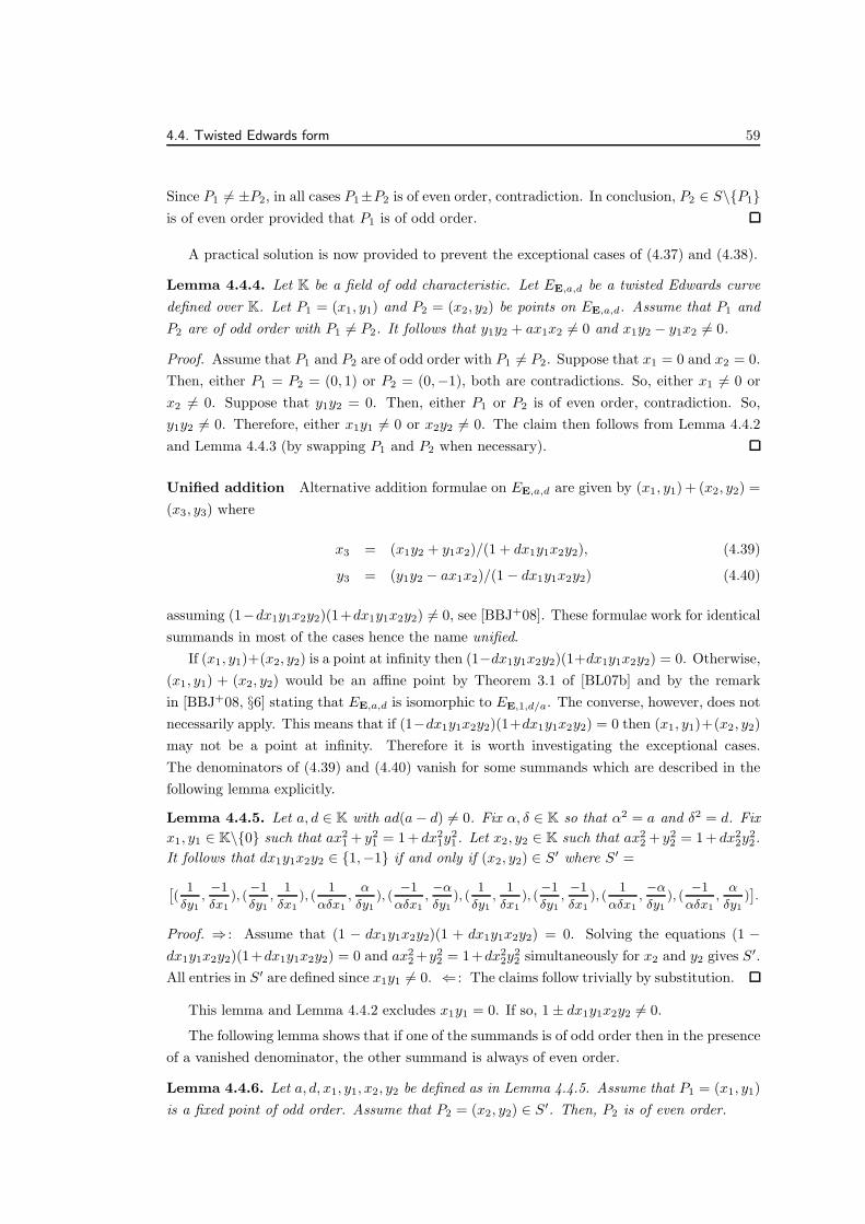
4.4. Twisted Edwards form 59
Since P1 6= ±P2, in all cases P1±P2 is of even order, contradiction. In conclusion, P2 ∈ S\P1is of even order provided that P1 is of odd order.
A practical solution is now provided to prevent the exceptional cases of (4.37) and (4.38).
Lemma 4.4.4. Let K be a field of odd characteristic. Let EE,a,d be a twisted Edwards curve
defined over K. Let P1 = (x1, y1) and P2 = (x2, y2) be points on EE,a,d. Assume that P1 and
P2 are of odd order with P1 6= P2. It follows that y1y2 + ax1x2 6= 0 and x1y2 − y1x2 6= 0.
Proof. Assume that P1 and P2 are of odd order with P1 6= P2. Suppose that x1 = 0 and x2 = 0.
Then, either P1 = P2 = (0, 1) or P2 = (0,−1), both are contradictions. So, either x1 6= 0 or
x2 6= 0. Suppose that y1y2 = 0. Then, either P1 or P2 is of even order, contradiction. So,
y1y2 6= 0. Therefore, either x1y1 6= 0 or x2y2 6= 0. The claim then follows from Lemma 4.4.2
and Lemma 4.4.3 (by swapping P1 and P2 when necessary).
Unified addition Alternative addition formulae on EE,a,d are given by (x1, y1) + (x2, y2) =
(x3, y3) where
x3 = (x1y2 + y1x2)/(1 + dx1y1x2y2), (4.39)
y3 = (y1y2 − ax1x2)/(1− dx1y1x2y2) (4.40)
assuming (1−dx1y1x2y2)(1+dx1y1x2y2) 6= 0, see [BBJ+08]. These formulae work for identical
summands in most of the cases hence the name unified.
If (x1, y1)+(x2, y2) is a point at infinity then (1−dx1y1x2y2)(1+dx1y1x2y2) = 0. Otherwise,
(x1, y1) + (x2, y2) would be an affine point by Theorem 3.1 of [BL07b] and by the remark
in [BBJ+08, §6] stating that EE,a,d is isomorphic to EE,1,d/a. The converse, however, does not
necessarily apply. This means that if (1−dx1y1x2y2)(1+dx1y1x2y2) = 0 then (x1, y1)+(x2, y2)
may not be a point at infinity. Therefore it is worth investigating the exceptional cases.
The denominators of (4.39) and (4.40) vanish for some summands which are described in the
following lemma explicitly.
Lemma 4.4.5. Let a, d ∈ K with ad(a− d) 6= 0. Fix α, δ ∈ K so that α2 = a and δ2 = d. Fix
x1, y1 ∈ K\0 such that ax21 + y2
1 = 1+ dx21y
21. Let x2, y2 ∈ K such that ax2
2 + y22 = 1+ dx2
2y22.
It follows that dx1y1x2y2 ∈ 1,−1 if and only if (x2, y2) ∈ S′ where S′ =
ˆ
(1
δy1,−1
δx1
), (−1
δy1,
1
δx1
), (1
αδx1
,α
δy1), (−1
αδx1
,−αδy1
), (1
δy1,
1
δx1
), (−1
δy1,−1
δx1
), (1
αδx1
,−αδy1
), (−1
αδx1
,α
δy1)˜
.
Proof. ⇒ : Assume that (1 − dx1y1x2y2)(1 + dx1y1x2y2) = 0. Solving the equations (1 −dx1y1x2y2)(1+dx1y1x2y2) = 0 and ax2
2 +y22 = 1+dx2
2y22 simultaneously for x2 and y2 gives S′.
All entries in S′ are defined since x1y1 6= 0. ⇐ : The claims follow trivially by substitution.
This lemma and Lemma 4.4.2 excludes x1y1 = 0. If so, 1± dx1y1x2y2 6= 0.
The following lemma shows that if one of the summands is of odd order then in the presence
of a vanished denominator, the other summand is always of even order.
Lemma 4.4.6. Let a, d, x1, y1, x2, y2 be defined as in Lemma 4.4.5. Assume that P1 = (x1, y1)
is a fixed point of odd order. Assume that P2 = (x2, y2) ∈ S′. Then, P2 is of even order.

60 Chapter 4. Group law in affine coordinates
Proof. In [BL07b] (where a = 1) and later in [BBJ+08], it is proven that the points at infinity
(over the extension of K where they exist) are of even order. Assume that P1 = (x1, y1) is a
fixed point of odd order hence not a point at infinity. Suppose that P2 is of odd order hence
not a point at infinity. It follows that P1 ± P2, M = 2P1, and N = 2P2 are all of odd order
hence not points at infinity.
Assume that P2 ∈ S′. Then, dx1y1x2y2 ∈ 1,−1 by Lemma 4.4.5 and it follows that
P1 6= ±P2, for otherwise, dx21y
21 ∈ 1,−1 and P1 would be of even order, see Remark 4.4.1.
Note that x1, y1 6= 0 since dx1y1x2y2 ∈ 1,−1 (also true by definition). So, x2y2 =
±1/(dx1y1) are defined taking the signs independently. Using this relation together with
(4.39) gives
x(N) =2x2y2
1 + dx22y
22
=2 ±1
dx1y1
1 + d( ±1
dx1y1)2
= ± 2x1y11 + dx2
1y21
= ±x(M).
By the curve definition, y(M) = ±y(N) since |x(M)| = |x(N)|. Now,
• x(M) = x(N) and y(M) = y(N): M −N = (0, 1). So, M −N = 2P1 − 2P2 = 2(P1 − P2) = (0, 1).
• x(M) = x(N) and y(M) = −y(N): M+N = (0,−1). So, 2(M+N) = 2(2P1+2P2) = 4(P1+P2) = (0, 1).
• x(M) = −x(N) and y(M) = y(N): M + N = (0, 1). So, M + N = 2P1 + 2P2 = 2(P1 + P2) = (0, 1).
• x(M) = −x(N) and y(M) = −y(N): M −N = (0,−1). So, 2(M −N) = 2(2P1 − 2P2) = 4(P1 − P2) =
(0, 1).
Since P1 6= ±P2, in all cases P1 ± P2 is of even order, contradiction. In conclusion, P2 ∈ S′ is
of even order provided that P1 is of odd order.
In the following lemma, with reasonable assumptions, it is shown that exceptions can be
prevented regardless of any assumption on the curve constants.
Lemma 4.4.7. Let K be a field of odd characteristic. Let EE,a,d be a twisted Edwards curve
defined over K. Let P1 = (x1, y1) and P2 = (x2, y2) be points on EE,a,d. Assume that P1 and
P2 are of odd order. It follows that 1± dx1x2y1y2 6= 0.
Proof. Assume that P1 and P2 are of odd order. If x1y1x2y2 = 0 then 1 ± dx1y1x2y2 6= 0
as desired. If x1y1x2y2 6= 0 then the claim follows from Lemma 4.4.5 and Lemma 4.4.6 (by
swapping P1 and P2 when necessary).
Exception handling in the general case Algorithm 4.4.1 provides a complete addition on
all twisted Edwards curves. The correctness of the algorithm follows from two observations.
Firstly, when a point at infinity is involved as the sum or as one of the summands along the lines
2 to 41, it is tedious but straightforward to check that the output of the algorithm is correct
using the implicit technique mentioned at the start of the chapter. Line 1 conditionally swaps
the inputs to eliminate half of the input-wise symmetric branches. The second observation
is that glueing together the unified addition and the dedicated addition formulae is enough
to handle all exceptions when both of the summands and the sum are affine points. This
fact follows from Lemma 4.4.5 and Lemma 4.4.2 by observing that #(S′ ∩ S) = 4. This
means that if (x2, y2) ∈ S′ ∩ S then the output must be a point at infinity (lines 51 to 54)
since there are exactly four points at infinity. The remaining exceptional cases which occur
at (x2, y2) ∈ S′\(S′ ∩ S) are handled by the dedicated addition formulae (lines 43 and 44).

4.4. Twisted Edwards form 61
Algorithm 4.4.1: Addition law in affine coordinates for twisted Edwards form
input : P1, P2,Ω1,Ω2,Ω3,Ω4 ∈ EE,a,d(K) and fixed α, δ ∈ K such that α2 = a and δ2 = d.
output : P1 + P2.
if P1 ∈ Ω1, Ω2,Ω3,Ω4 then Pt ← P1, P1 ← P2, P2 ← Pt.1
if P2 = Ω1 then2
if P1 = Ω1 then return (0, 1).3
else if P1 = Ω2 then return (0,−1).4
else if P1 = Ω3 then return (−1/α, 0).5
else if P1 = Ω4 then return (1/α, 0).6
else if P1 = (0, 1) then return Ω1.7
else if P1 = (0,−1) then return Ω2.8
else if P1 = (−1/α, 0) then return Ω3.9
else if P1 = (1/α, 0) then return Ω4.10
else return (−1/(αδx1),−α/(δy1)).11
else if P2 = Ω2 then12
if P1 = Ω1 then return (0,−1).13
else if P1 = Ω2 then return (0, 1).14
else if P1 = Ω3 then return (1/α, 0).15
else if P1 = Ω4 then return (−1/α, 0).16
else if P1 = (0,−1) then return Ω1.17
else if P1 = (0, 1) then return Ω2.18
else if P1 = (1/α, 0) then return Ω3.19
else if P1 = (−1/α, 0) then return Ω4.20
else return (1/(αδx1), α/(δy1)).21
else if P2 = Ω3 then22
if P1 = Ω1 then return (−1/α, 0).23
else if P1 = Ω2 then return (1/α, 0).24
else if P1 = Ω3 then return (0,−1).25
else if P1 = Ω4 then return (0, 1).26
else if P1 = (1/α, 0) then return Ω1.27
else if P1 = (−1/α, 0) then return Ω2.28
else if P1 = (0, 1) then return Ω3.29
else if P1 = (0,−1) then return Ω4.30
else return (1/(δy1),−1/(δx1)).31
else if P2 = Ω4 then32
if P1 = Ω1 then return (1/α, 0).33
else if P1 = Ω2 then return (−1/α, 0).34
else if P1 = Ω3 then return (0, 1).35
else if P1 = Ω4 then return (0,−1).36
else if P1 = (−1/α, 0) then return Ω1.37
else if P1 = (1/α, 0) then return Ω2.38
else if P1 = (0,−1) then return Ω3.39
else if P1 = (0, 1) then return Ω4.40
else return (−1/(δy1), 1/(δx1)).41
else if (y1y2 + ax1x2)(x1y2 − y1x2) 6= 0 then42
x3 ← (x1y1 + x2y2)/(y1y2 + ax1x2).43
y3 ← (x1y1 − x2y2)/(x1y2 − y1x2).44
return (x3, y3).45
else if (1− dx1x2y1y2)(1 + dx1x2y1y2) 6= 0 then46
x3 ← (x1y2 + y1x2)/(1 + dx1x2y1y2).47
y3 ← (y1y2 − ax1x2)/(1 − dx1x2y1y2).48
return (x3, y3).49
else50
if P2 = (1/(αδx1),−α/(δy1)) then return Ω1.51
else if P2 = (−1/(αδx1), α/(δy1)) then return Ω2.52
else if P2 = (1/(δy1), 1/(δx1)) then return Ω3.53
else return Ω4.54
end55

62 Chapter 4. Group law in affine coordinates
Similarly the exceptions at (x2, y2) ∈ S− (S′∩S) are handled by the unified addition formulae
(lines 47 and 48).
The points at infinity on the desingularized projective closure of EE,a,d are not defined over
K if d is not a square in K and a is a square in K, see [BBJ+08]. Having noted this, it was proven
in [BL07b] (where a = 1) and later in [BBJ+08] that the unified addition formulae (4.39) and
(4.40) are complete provided that d is not a square in K and a is a square in K. Algorithm 4.4.1
complies with the completeness criterion since only the lines 47 to 49 are necessary in this case.
Note that the assumptions on the curve constants a and d limit the number of curves in twisted
Edwards form for which the unified addition formulae are complete. In [BBJ+08] such curves
are named complete Edwards curves.
Algorithm 4.4.1 also complies with Lemma 4.4.7. If P1 and P2 are points of odd order only
the lines 47 to 49 are necessary. This technique applies to all twisted Edwards curves.
Algorithm 4.4.1 also complies with Lemma 4.4.4. If P1 and P2 are distinct points of odd
order then only the lines 43 to 45 are necessary. This technique applies to all twisted Edwards
curves. The doubling formulae (4.35) and (4.36) are enough to handle the special case P1 = P2.
More formulae Using the tools of Chapter 3, it is possible to derive other low-degree
addition formulae;
x3 =e(x1y1 + x2y2) + f(x1y2 + y1x2)
e(y1y2 + ax1x2) + f(1 + dx1y1x2y2), (4.41)
y3 =g(x1y1 − x2y2) + h(y1y2 − ax1x2)
g(x1y2 − y1x2) + h(1− dx1y1x2y2)(4.42)
assuming that (e(y1y2 + ax1x2) + f(1 + dx1y1x2y2))(g(x1y2 − y1x2) + h(1 − dx1y1x2y2)) 6= 0
where e, f, g, h ∈ K such that efgh 6= 0. These formulae tend to include more subexpressions
which are not commonly shared. Therefore, their evaluation turns out to be more costly and
thus not considered hereafter.
Literature notes Other results related to the affine formulae for twisted Edwards curves
can be found in the literature. Bernstein et al. used Edwards curves (i.e. a = 1) in the
ECM method of integer factorization in [BBLP08]. Bernstein et al. introduced the shape
d1(x+y)+d2(x2+y2) = (x+x2)(y+y2) and presented results on the arithmetic of these curves
when char(K) = 2 in [BLR08]. These curve are named binary Edwards curves. In chronological
order, Das and Sarkar [DS08], Ionica and Joux [IJ08], and Arene et al. [ALNR09] introduced
successively faster formulae for pairing computations. The results in [DS08] and [IJ08] are
based on the unified addition formulae and the doubling formulae with a = 1. The results
in [ALNR09] are based on the dedicated addition formulae and the doubling formulae. The
same reference also provided a geometric interpretation of the group law on twisted Edwards
curves.

4.5. Twisted Jacobi intersection form 63
4.5 Twisted Jacobi intersection form
This section presents the group law on EI,b,a in affine coordinates. It also investigates the
exceptional summands for each set of formulae and provides a complete addition algorithm
for all twisted Jacobi intersection curves by properly handling an entire set of divide-by-zero
exceptions. In addition, practical ways of preventing these exceptions are explained.
Throughout this section, let K be a field of odd characteristic. Recall from Chapter 2 that
a twisted Jacobi intersection curve is defined by
EI,b,a : bs2 + c2 = 1, as2 + d2 = 1
where a, b ∈ K with ab(a− b) 6= 0. Assume that both −a and −b are squares in K. Recall from
Chapter 2 that the set of K-rational points on EI,b,a is defined by
EI,b,a(K) = (s, c, d) ∈ K3 | bs2 + c2 = 1, as2 + d2 = 1 ∪ Ω1,Ω2,Ω3,Ω4
where Ω1,Ω2,Ω3,Ω4 are points at infinity.
Identity element and negation The identity element can suitably be taken as (0, 1, 1).
Let (s1, c1, d1) be a point on EI,b,a. The negative of (s1, c1, d1) is (−s1, c1, d1).
Doubling The doubling formulae on EI,b,a is given by [2](s1, c1, d1) = (s3, c3, d3) where
s3 = 2s1c1d1/(c21 + bs21d
21), (4.43)
c3 = (c21 − bs21d21)/(c
21 + bs21d
21), (4.44)
d3 = (2d21 − c21 − bs21d2
1)/(c21 + bs21d
21). (4.45)
assuming that c21 + bs21d21 6= 0. These formulae are of minimal total degree and do not depend
on the curve constants a and b. By the curve equation the denominator c21 +bs21d21 is equivalent
to 1− abs41 or c21 + d21 − c21d2
1 or d21 + as21c
21. These denominators can also be used.
The points (0,−1, 1), (0, 1,−1), and (0,−1,−1) are of order 2. This can be determined by
solving bs21 + c21 = 1, as21 + d21 = 1 and (s3, c3, d3) = (0, 1, 1) for s1, c1, and d1 where s3, c3, and
d3 are given by (4.43), (4.44), and (4.45).
The four points of the form having the c-coordinates equal to zero are of order 4. This can
be determined by solving bs21 + c21 = 1, as21 + d21 = 1 and (s3, c3, d3) = (0,−1, 1) for s1, c1, and
d1. Another set of four points having the d-coordinates equal to zero are also of order 4. This
can be determined by solving bs21 + c21 = 1, as21 + d21 = 1 and (s3, c3, d3) = (0, 1,−1) for s1, c1,
and d1. There are twelve points of order 4 in total (over a sufficiently large finite extension of
K). Therefore the remaining four points of order 4 have to be the points at infinity Ω1, Ω2,
Ω3, and Ω4. These points are the only exceptions of (4.43), (4.44), and (4.45). The following
remark is immediate.
Remark 4.5.1. [2](s1, c1, d1) is a point at infinity if and only if c21 + bs21d21 = 0.
Remark 4.5.1 does not extend to the case of generic additions. However, it is still useful in

64 Chapter 4. Group law in affine coordinates
proving some lemmas regarding the generic addition formulae which will be presented next.
Dedicated addition Further let (s2, c2, d2) be a point on EI,b,a. The addition formulae on
EI,b,a are given by (s1, c1, d1) + (s2, c2, d2) = (s3, c3, d3) where
s3 = (s21 − s22)/(s1c2d2 − c1d1s2), (4.46)
c3 = (s1c1d2 − d1s2c2)/(s1c2d2 − c1d1s2), (4.47)
d3 = (s1d1c2 − c1s2d2)/(s1c2d2 − c1d1s2) (4.48)
assuming that s1c2d2 − c1d1s2 6= 0. These formulae are of minimal total degree and do not
depend on the curve constants a and b. These formulae do not work for identical summands
hence the name dedicated.
If (s1, c1, d1) + (s2, c2, d2) is a point at infinity then s1c2d2 − c1d1s2 = 0. Otherwise,
(s1, c1, d1) + (s2, c2, d2) would be an affine point since it can be shown using the relations
bs21 + c21 = 1, as21 + d21 = 1 and bs22 + c22 = 1, as22 + d2
2 = 1 that the algebraic expressions for
(s3, c3, d3) satisfy bs23 + c23 = 1, as23 + d23 = 1. The converse, however, does not necessarily
apply. This means that if s1c2d2 − c1d1s2 = 0 then (s1, c1, d1) + (s2, c2, d2) may not be a
point at infinity. Therefore it is worth investigating the exceptional cases. The denominators
of (4.46), (4.47), and (4.48) vanish for some summands which are described in the following
lemma explicitly.
Lemma 4.5.2. Let a, b ∈ K with ab(a− b) 6= 0. Fix α, β ∈ K so that α2 = −a and β2 = −b.Fix s1 ∈ K\0 and c1, d1 ∈ K such that bs21 + c21 = 1 and as21 + d2
1 = 1. Let s2, c2, d2 ∈ K such
that bs22 + c22 = 1, as22 + d22 = 1. Now, s1c2d2 − c1d1s2 = 0 if and only if (s2, c2, d2) ∈ S where
S =ˆ
(s1, c1, d1), (s1,−c1,−d1), (−s1,−c1, d1), (−s1, c1,−d1),
(1
αβs1,d1
αs1,c1βs1
), (1
αβs1,−d1
αs1,−c1βs1
), (−1
αβs1,−d1
αs1,c1βs1
), (−1
αβs1,d1
αs1,−c1βs1
)˜
.
Proof. ⇒ : Assume that s1c2d2 − c1d1s2 = 0. Solving the equations s1c2d2 − c1d1s2 = 0,
bs22 + c22 = 1 and as22 + d22 = 1 simultaneously for s2, c2, and d2 gives S. All entries in S are
defined since s1 6= 0. ⇐ : The claims follow trivially by substitution.
The following lemma shows that if one of the summands is of odd order then in the presence
of an exception, the other summand is always of even order.
Lemma 4.5.3. Let a, b, s1, c1, d1, s2, c2, d2 be defined as in Lemma 4.5.2. Assume that P1 =
(s1, c1, d1) is a fixed point of odd order. Assume that P2 ∈ S\P1. Then P2 is of even order.
Proof. Note that points at infinity (over the extension of K where they exist) are of even order.
Assume that P1 = (s1, c1, d1) is a fixed point of odd order hence not a point at infinity. Suppose
that P2 is of odd order hence not a point at infinity. It follows that P1 ± P2, M = 2P1, and
N = 2P2 are all of odd order hence not points at infinity.
Assume that P2 ∈ S\P1. So, P1 6= P2. Plus, s1c2d2 − c1d1s2 = 0 by Lemma 4.5.2. It
follows that P1 6= −P2, for otherwise, s1c2d2−c1d1s2 = 2s1c1d1 = 0 which means that c1d1 = 0
since s1 6= 0. But then P1 would be of even order.

4.5. Twisted Jacobi intersection form 65
It is possible to continue in a similar way used in the previous sections however this time
computer algebra will be used. The following Maple script verifies that s(M)2 = s(N)2,
c(M)2 = c(N)2, and d(M)2 = d(N)2.
> Q:=(s,c,d)->(b*s^2+c^2-1,a*s^2+d^2-1):
> sM:=2*s1*c1*d1/(c1^2+b*s1^2*d1^2):
> cM:=(c1^2-b*s1^2*d1^2)/(c1^2+b*s1^2*d1^2):
> dM:=(2*d1^2-c1^2-b*s1^2*d1^2)/(c1^2+b*s1^2*d1^2):
> sN:=2*s2*c2*d2/(c2^2+b*s2^2*d2^2):
> cN:=(c2^2-b*s2^2*d2^2)/(c2^2+b*s2^2*d2^2):
> dN:=(2*d2^2-c2^2-b*s2^2*d2^2)/(c2^2+b*s2^2*d2^2):
> simplify([sM^2-sN^2,cM^2-cN^2,dM^2-dN^2],[s1*c2*d2-c1*d1*s2=0,Q(s1,c1,d1),Q(s2,c2,d2)]);
[0,0,0]
Therefore, s(M) = ±s(N), c(M) = ±c(N), and d(M) = ±d(N) taking the signs independently.Now,
• s(M) = s(N), c(M) = c(N), d(M) = d(N): M −N = (0, 1, 1). So, M −N = 2P1 − 2P2 = 2(P1 − P2) =
(0, 1, 1);
• s(M) = −s(N), c(M) = c(N), d(M) = d(N): M +N = (0, 1, 1). So, M +N = 2P1 +2P2 = 2(P1 +P2) =
(0, 1, 1);
• s(M) = s(N), c(M) = −c(N), d(M) = d(N): M + N = (0,−1, 1). So, M + N = 2(2P1 + 2P2) =
4(P1 + P2) = (0, 1, 1);
• s(M) = −s(N), c(M) = −c(N), d(M) = d(N): M − N = (0,−1, 1). So, M − N = 2(2P1 + 2P2) =
4(P1 + P2) = (0, 1, 1);
• s(M) = s(N), c(M) = c(N), d(M) = −d(N): M + N = (0, 1,−1). So, M + N = 2(2P1 + 2P2) =
4(P1 + P2) = (0, 1, 1);
• s(M) = −s(N), c(M) = c(N), d(M) = −d(N): M − N = (0, 1,−1). So, M − N = 2(2P1 + 2P2) =
4(P1 + P2) = (0, 1, 1);
• s(M) = s(N), c(M) = −c(N), d(M) = −d(N): M − N = (0,−1,−1). So, M − N = 2(2P1 − 2P2) =
4(P1 − P2) = (0, 1, 1); and
• s(M) = −s(N), c(M) = −c(N), d(M) = −d(N): M + N = (0,−1,−1). So, M + N = 2(2P1 − 2P2) =
4(P1 − P2) = (0, 1, 1).
Since P1 6= ±P2, in all cases P1±P2 is of even order, contradiction. In conclusion, P2 ∈ S\P1is of even order provided that P1 is of odd order.
A practical solution is now provided to prevent the exceptional cases of (4.46), (4.47), and
(4.48).
Lemma 4.5.4. Let K be a field of odd characteristic. Let EI,b,a be a twisted Jacobi intersection
curve defined over K. Let P1 = (s1, c1, d1) and P2 = (s2, c2, d2) be points on EI,b,a. Assume
that P1 and P2 are of odd order with P1 6= P2. It follows that s1c2d2 − c1d1s2 6= 0.
Proof. Assume that P1 and P2 are of odd order with P1 6= P2. Suppose that s1 = 0 and s2 = 0.
Then, P1 = P2 = (0, 1, 1), contradiction. So, either s1 6= 0 or s2 6= 0. The claim then follows
from Lemma 4.5.2 and Lemma 4.5.3 (by swapping P1 and P2 when necessary).

66 Chapter 4. Group law in affine coordinates
Unified addition Alternative addition formulae on EI,b,a are given by (s1, c1, d1) +
(s2, c2, d2) = (s3, c3, d3) where
s3 = (s1c2d2 + c1d1s2)/(1− abs21s22), (4.49)
c3 = (c1c2 − bs1d1s2d2)/(1− abs21s22), (4.50)
d3 = (d1d2 − as1c1s2c2)/(1− abs21s22) (4.51)
assuming that 1 − abs21s22 6= 0. These formulae work for identical summands in most of the
cases hence the name unified.
If (s1, c1, d1)+(s2, c2, d2) is a point at infinity then 1−abs21s22 = 0. Otherwise, (s1, c1, d1)+
(s2, c2, d2) would be an affine point since it can be shown using the relations bs21 + c21 =
1, as21 + d21 = 1 and bs22 + c22 = 1, as22 + d2
2 = 1 that the algebraic expressions for (s3, c3, d3)
satisfy bs23 + c23 = 1, as23 + d23 = 1. The converse, however, does not necessarily apply. This
means that if 1 − abs21s22 = 0 then (s1, c1, d1) + (s2, c2, d2) may not be a point at infinity.
Therefore it is worth investigating the exceptional cases. The denominators of (4.49), (4.50),
and (4.51) vanish for some summands which are described in the following lemma explicitly.
Lemma 4.5.5. Let a, b, s1, c1, d1, s2, c2, d2 be defined as in Lemma 4.5.2. It follows that 1 −abs21s
22 6= 0 if and only if (s2, c2, d2) ∈ S′ where
S′ =ˆ
(1
αβs1,−d1
αs1,c1βs1
), (1
αβs1,d1
αs1,−c1βs1
), (−1
αβs1,d1
αs1,c1βs1
), (−1
αβs1,−d1
αs1,−c1βs1
)
(1
αβs1,d1
αs1,c1βs1
), (1
αβs1,−d1
αs1,−c1βs1
), (−1
αβs1,−d1
αs1,c1βs1
), (−1
αβs1,d1
αs1,−c1βs1
)˜
.
Proof. ⇒ : Assume that 1 − abs21s22 = 0. Solving the equations 1− abs21s22 = 0, bs22 + c22 = 1,
and as22 + d22 = 1 simultaneously for s2, c2, and d2 gives S′. All entries in S′ are defined since
s1 6= 0. ⇐ : The claims follow trivially by substitution.
This lemma and Lemma 4.5.2 excludes s1 = 0. If so, 1− abs21s22 6= 0.
The following lemma shows that if one of the summands is of odd order then in the presence
of a vanished denominator, the other summand is always of even order.
Lemma 4.5.6. Let a, b, s1, c1, d1, s2, c2, d2 be defined as in Lemma 4.5.5. Assume that P1 =
(s1, c1, d1) is a fixed point of odd order. Assume that P2 = (s2, c2, d2) ∈ S′. Then, P2 is of
even order.
Proof. The proof is similar to the proof of Lemma 4.5.3. The only difference is that the phrase
s1*c2*d2-c1*d1*s2=0 should be changed to 1-a*b*s1*s1*s2*s2=0 in the Maple script of the
proof of Lemma 4.5.3 and the claim follows.
In the following lemma, with reasonable assumptions, it is shown that exceptions can be
prevented regardless of any assumption on the curve constants.
Lemma 4.5.7. Let K be a field of odd characteristic. Let EI,b,a be a twisted Jacobi intersection
curve defined over K. Let P1 = (s1, c1, d1) and P2 = (s2, c2, d2) be points on EI,b,a. Assume
that P1 and P2 are of odd order. It follows that 1− abs21s22 6= 0.

4.5. Twisted Jacobi intersection form 67
Proof. Assume that P1 and P2 are of odd order. If s1s2 = 0 then 1− abs21s22 6= 0 as desired. If
s1s2 6= 0 then the claim follows from Lemma 4.5.5 and Lemma 4.5.6 (by swapping P1 and P2
when necessary).
Exception handling in the general case Algorithm 4.5.1 provides a complete addition
on all twisted Jacobi intersection curves. The correctness of the algorithm follows from
two observations. Firstly, when a point at infinity is involved as the sum or as one of the
summands along lines 2 to 13, it is tedious but straightforward to check that the output of the
algorithm is correct using the implicit technique mentioned at the start of the chapter. Line 1
conditionally swaps the inputs to eliminate half of the input-wise symmetric branches. The
second observation is that glueing together the unified addition and the dedicated addition
formulae is enough to handle all exceptions when both of the summands and the sum are affine
points. This fact follows from Lemma 4.5.5 and Lemma 4.5.2 by observing that #(S′∩S) = 4.
This means that if (s2, c2, d2) ∈ S′ ∩ S then the output must be a point at infinity (lines 53
to 56) since there are exactly four points at infinity. The remaining exceptional cases which
occur at (s2, c2, d2) ∈ S′\(S′ ∩ S) are handled by the dedicated addition formulae (lines 43 to
45). Similarly the exceptions at (s2, c2, d2) ∈ S\(S′ ∩ S) are handled by the unified addition
formulae (lines 48 to 50).
The points at infinity on the projective closure of EI,b,a are not defined over K if a is not a
square in K. Having noted this, the following lemma implies that these addition formulae are
complete if a is not a square in K.
Lemma 4.5.8. Let a, b, s1, s2 ∈ K. Assume that ab is non-square. Then 1− abs21s22 6= 0.
Proof. See the proof of Lemma 4.2.8 in §4.2.
Algorithm 4.5.1 complies with the completeness criterion since only the lines 48 to 50 are
necessary in this case. Note that the assumption on the curve constants a and d limits the
number of curves in twisted Jacobi intersection form for which the unified addition formulae
are complete.
Algorithm 4.5.1 also complies with Lemma 4.5.7. If P1 and P2 are points of odd order then
all branches are eliminated and the lines 48 to 50 suffice. This technique applies to all twisted
Jacobi intersection curves.
Algorithm 4.5.1 also complies with Lemma 4.5.4. If P1 and P2 are distinct points of odd
order then all branches are eliminated and the lines 43 to 45 suffice. This technique applies
to all twisted Jacobi intersection curves. The doubling formulae (4.55), (4.56), and (4.57) are
enough to handle the special case P1 = P2.
More formulae Using the tools of Chapter 3, it is possible to derive many more low-degree
addition formulae. In the case of doubling, the numerators can also be written in several
alternative ways. However, there exist no formulae of lower total degree to compute any of
these affine coordinates. The following examples are specifically chosen since each of them
share many common subexpressions among their coordinates. More common subexpressions
often reduces the complexity of the evaluation. One set of formulae (independent of a and b)
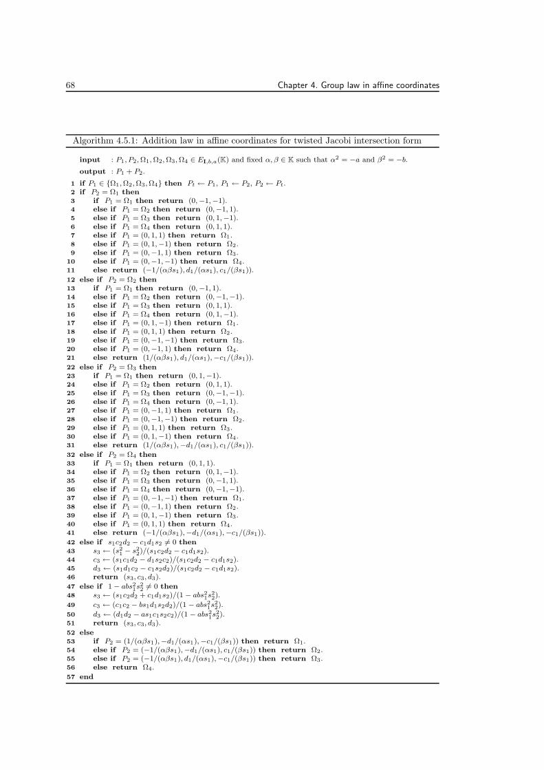
68 Chapter 4. Group law in affine coordinates
Algorithm 4.5.1: Addition law in affine coordinates for twisted Jacobi intersection form
input : P1, P2, Ω1, Ω2, Ω3, Ω4 ∈ EI,b,a(K) and fixed α, β ∈ K such that α2 = −a and β2 = −b.
output : P1 + P2.
if P1 ∈ Ω1,Ω2,Ω3,Ω4 then Pt ← P1, P1 ← P2, P2 ← Pt.1
if P2 = Ω1 then2
if P1 = Ω1 then return (0,−1,−1).3
else if P1 = Ω2 then return (0,−1, 1).4
else if P1 = Ω3 then return (0, 1,−1).5
else if P1 = Ω4 then return (0, 1, 1).6
else if P1 = (0, 1, 1) then return Ω1.7
else if P1 = (0, 1,−1) then return Ω2.8
else if P1 = (0,−1, 1) then return Ω3.9
else if P1 = (0,−1,−1) then return Ω4.10
else return (−1/(αβs1), d1/(αs1), c1/(βs1)).11
else if P2 = Ω2 then12
if P1 = Ω1 then return (0,−1, 1).13
else if P1 = Ω2 then return (0,−1,−1).14
else if P1 = Ω3 then return (0, 1, 1).15
else if P1 = Ω4 then return (0, 1,−1).16
else if P1 = (0, 1,−1) then return Ω1.17
else if P1 = (0, 1, 1) then return Ω2.18
else if P1 = (0,−1,−1) then return Ω3.19
else if P1 = (0,−1, 1) then return Ω4.20
else return (1/(αβs1), d1/(αs1),−c1/(βs1)).21
else if P2 = Ω3 then22
if P1 = Ω1 then return (0, 1,−1).23
else if P1 = Ω2 then return (0, 1, 1).24
else if P1 = Ω3 then return (0,−1,−1).25
else if P1 = Ω4 then return (0,−1, 1).26
else if P1 = (0,−1, 1) then return Ω1.27
else if P1 = (0,−1,−1) then return Ω2.28
else if P1 = (0, 1, 1) then return Ω3.29
else if P1 = (0, 1,−1) then return Ω4.30
else return (1/(αβs1),−d1/(αs1), c1/(βs1)).31
else if P2 = Ω4 then32
if P1 = Ω1 then return (0, 1, 1).33
else if P1 = Ω2 then return (0, 1,−1).34
else if P1 = Ω3 then return (0,−1, 1).35
else if P1 = Ω4 then return (0,−1,−1).36
else if P1 = (0,−1,−1) then return Ω1.37
else if P1 = (0,−1, 1) then return Ω2.38
else if P1 = (0, 1,−1) then return Ω3.39
else if P1 = (0, 1, 1) then return Ω4.40
else return (−1/(αβs1),−d1/(αs1),−c1/(βs1)).41
else if s1c2d2 − c1d1s2 6= 0 then42
s3 ← (s21− s2
2)/(s1c2d2 − c1d1s2).43
c3 ← (s1c1d2 − d1s2c2)/(s1c2d2 − c1d1s2).44
d3 ← (s1d1c2 − c1s2d2)/(s1c2d2 − c1d1s2).45
return (s3, c3, d3).46
else if 1− abs21s226= 0 then47
s3 ← (s1c2d2 + c1d1s2)/(1 − abs21s22).48
c3 ← (c1c2 − bs1d1s2d2)/(1 − abs21s2
2).49
d3 ← (d1d2 − as1c1s2c2)/(1 − abs21s22).50
return (s3, c3, d3).51
else52
if P2 = (1/(αβs1),−d1/(αs1),−c1/(βs1)) then return Ω1.53
else if P2 = (−1/(αβs1),−d1/(αs1), c1/(βs1)) then return Ω2.54
else if P2 = (−1/(αβs1), d1/(αs1),−c1/(βs1)) then return Ω3.55
else return Ω4.56
end57

4.6. Conclusion 69
is given as follows.
s3 = 2s1c1d1/(c21 + d2
1 − c21d21), (4.52)
c3 = (c21 − d21 + c21d
21)/(c
21 + d2
1 − c21d21), (4.53)
d3 = (d21 − c21 + c21d
21)/(c
21 + d2
1 − c21d21). (4.54)
Another set of formulae is given as follows.
s3 = 2s1c1d1/(1− abs41), (4.55)
c3 = (c21 − bs21d21)/(1− abs41), (4.56)
d3 = (d21 − as21c21)/(1− abs41) (4.57)
Yet another set of formulae (independent of b) is given as follows.
s3 = 2s1c1d1/(d21 + as21c
21), (4.58)
c3 = (2c21 − d21 − as21c21)/(d2
1 + as21c21), (4.59)
d3 = (d21 − as21c21)/(d2
1 + as21c21). (4.60)
Some of these formulae will be used later in Chapter 5. It is possible to provide many more
examples. Indeed some alternative examples will be further mentioned in the following chapter
in which the aim is to investigate inversion-free operation counts on projective coordinates.
In the case of unified addition, observe that the denominator contains s2i . Using the defining
equations 1− abs21s22 can also be written as 1− as21(1 − c22) = 1 − as21 + as21c22 = d2
1 + as21c22 or
1−bs21(1−d22) = 1−bs21 +bs21d
22 = c21 +bs21d
22 or 1− (a/b)(1−c21)(1−c22) = 1− (a/b)+(a/b)c21 +
(a/b)c22 − (a/b)c21c22 or 1− (b/a)(1− d2
1)(1− d22) = 1− (b/a) + (b/a)d2
1 + (b/a)d22 − (b/a)d2
1d22 or
1− (1− c21)(1− d22) = c21 + d2
2− c21d22. There exists even more alternatives. However all of these
denominators have a total degree of 4. Plus, the exceptional cases for all of these denominators
are the same. Similar arguments also apply to the case of dedicated addition.
Literature notes Other results related to the affine formulae for twisted Jacobi intersection
form can be found in the literature. The group law on Jacobi intersection curves are typically
derived directly from Jacobi elliptic functions, cf. [Jac29], [WW27], [CC86], and [BJ03a].
4.6 Conclusion
This chapter has provided low-total-degree formulae for elliptic curves in five basic forms of
elliptic curves, namely, short Weierstrass form (§4.1), extended Jacobi quartic form (§4.2),
twisted Hessian form (§4.3), twisted Edwards form (§4.4), and twisted Jacobi intersection form
(§4.5). Besides bringing various formulae together in one chapter, the arithmetic properties
of these formulae have also been studied algebraically. This is achieved by the determination
of exceptional summands explicitly, the showing of how exceptional cases (such as additions
involving the points at infinity) can be handled, the clarification of how these exceptions

70 Chapter 4. Group law in affine coordinates
can be prevented under reasonable assumptions, and a complete addition algorithm in affine
coordinates.
Complete addition by exception handling Although the complete addition algorithms
on Weierstrass curves were well documented in the literature, other representations had
only been studied in the case of some particular addition formulae and in many resources
the exceptional situations were simply omitted. This chapter has studied the topic from
a wider perspective. In particular, complete addition algorithms; Algorithm 4.2.1 in §4.2,
Algorithm 4.3.1 in §4.3 Algorithm 4.4.1 in §4.4, Algorithm 4.5.1 in §4.5, have been developed
for the first time.
In order to build these algorithms each section has developed two alternative formulae
covering the affine part of the curve. By covering the affine part it is meant that (the sequence
of points) S′∩S composed of element(s) forcing the condition P1 +P2 being a point at infinity
at an occurrence of a vanished denominator. See the lemmas in each section for detail. In fact,
the addition of an affine point (x1, y1) with one of the entries in the first half of S′ (or S) yields
an affine point although they produce division-by-zero exceptions with the relevant formulae.
The second half of entries also produce division-by-zero exceptions but the sum this time is
a point at infinity. These facts have been left implicit in the text to minimize repetition but
explicitly used while designing the complete addition algorithms for elliptic curves covered by
a particular form.
Complete addition by assumption(s) on the curve constant(s) Excluding the
Weierstrass form, new complete addition formulae are provided for each form using only a
single set of addition formulae. This property was first stated for some Edwards curves by
Bernstein and Lange in [BL07b]. Later the same idea was extended to suitable classes of elliptic
curves in twisted Edwards form in [BBJ+08] and to twisted Hessian form in [BL07a]. This
chapter has extended the same idea for suitable classes of elliptic curves in extended Jacobi
quartic and twisted Jacobi intersection forms, see §4.2 and §4.5. This technique forces the
point(s) at infinity to be defined over a proper extension of K but not over K itself. Therefore,
all points on the selected curve are affine points. The second part of the technique is composed
of finding a single set of addition formulae with denominators which cannot vanish for any pair
of summands.
Exception prevention At this point, having dedicated addition formulae which do not work
for some special summands might seem unnecessary. However, it will be shown in Chapter 5
that dedicated addition formulae lead to inversion-free algorithms which are as fast or even
faster than unified addition formulae. For simplicity in implementations, it is desirable to
have a condition for which the number of exceptional cases is minimal when using dedicated
addition formulae. Each section has introduced sufficient assumptions to have P1 = P2 as the
only exceptional case to be handled. (Of course, in the case of short Weierstrass form, the point
at infinity is also handled separately since it is always involved in the arithmetic as the identity
element.) In speed oriented implementations, distinguishing P1 = P2 is no problem because
it is a standard method to switch to faster doubling formulae in inversion-free coordinate

4.6. Conclusion 71
systems, see Chapter 5. In addition, the same technique removes all exceptional cases for the
unified addition formulae under suitable assumptions. In cryptographic applications, attention
is typically restricted to a large prime order subgroup of the curve. This criterion covers a
variety of different assumptions by further simplifying the exception prevention techniques
introduced in this chapter.

72 Chapter 4. Group law in affine coordinates

Chapter 5
Group law in projective
coordinates
Elliptic curves became increasingly employed in cryptology in the 1980’s, and since then there
has been a series of incremental studies to speed up the arithmetic of elliptic curves. This
chapter uses the tools from Chapter 3 and the group laws in affine coordinates from Chapter 4
in order to develop efficient group laws for elliptic curves over fields of large characteristic.
This chapter also provides a collection of selected algorithms from the literature to provide a
summary of the recent advances. The work is limited to studying five forms of elliptic curves
which have already been discussed in Chapter 4. It should be possible to extend this work to
many other curve models including those of small characteristic. This is left as future work.
In what follows some terms related to the group law on elliptic curves will be extensively
used. In particular, the term unified is used to emphasize that point addition formulae remain
valid when two input points are identical, see [CF05, §29.1.2]. Therefore, unified addition
formulae can be used for point doubling. The term dedicated is used to emphasize that point
addition formulae are not unified. The term re-addition is used to emphasize that a point
addition has already taken place and some of the previously computed data is cached, see
[BL07b]. The term redundant is used to emphasize that unnecessary computational data is
added to a projective representation of a point. The notations are adapted from [CMO98],
[BL07b], and [BBJ+08].
This chapter studies the arithmetic of selected elliptic curve forms in suitable coordinate
systems. Some coordinate systems (such as Qe in §5.2.2) are introduced in this chapter.
Some other coordinate systems (such as J in §5.5.2) are already studied in the literature.
Even for such systems this chapter introduces new algorithms which are practical in some
applications. For the quartic models ax2 + y2 = 1 + dx2y2 and y2 = dx4 + 2ax2 + 1, the
optimum speeds are achieved in a proposed approach using mixed homogeneous projective
coordinates. For each of these forms the extended homogeneous projective coordinates are
introduced which significantly improve the speed of point additions. The slowing down in
73

74 Chapter 5. Group law in projective coordinates
point doubling is remedied by mixing extended homogeneous projective coordinates with
homogeneous projective coordinates, see §5.1 and §5.2 for details. The twisted Hessian form
also exhibits some of these properties. However, in most situations, the proposed optimizations
in homogeneous projective coordinates are more interesting than the proposed optimizations in
extended homogeneous projective coordinates or modified homogeneous projective coordinates,
see §5.4. Jacobi intersection form can provide improved speeds in both homogeneous projective
coordinates and modified homogeneous projective coordinates. The speed of this form is close
to the speed of Jacobi quartic form, see §5.3. The arithmetic of Weierstrass form has been
extensively studied over decades. Therefore it is extremely unlikely to find faster algorithms
with arbitrary curve constants. On the other hand, it is still possible to improve the speed of
unified additions. The improvements for Weierstrass form are covered in §5.5. Each of these
section contains tables to compare literature results with the results from this thesis. The
entries which are not cited are the contributions of this thesis.
Since all formulae in this chapter are inversion-free they never cause division by zero
exceptions. However, this does not mean that the correct output will always be produced.
Some special inputs force all output coordinates be zero producing an n-tuple which is not
even a point on the underlying space. When this occurs, the results from Chapter 4 will be
recalled to show how to guarantee the correct output under some reasonable assumptions. If
those assumptions are not satisfied then the complete affine addition algorithms in Chapter 4
can be incorporated to explicitly handle all such special cases.
5.1 Twisted Edwards form
The arithmetic of twisted Edwards curves is studied under four different point representations
in this section, each system having its own advantages. The homogeneous projective coordinate
system from [BBJ+08] (also see [BL07b]) is revisited with additional results in §5.1.1. This
system allows fast doubling and additions and thus is interesting for efficient implementation.
Similarly, the inverted coordinate system from [BBJ+08] (also see [BL07c]) is revisited with
additional results in §5.1.2. This system allows faster additions in comparison to homogeneous
projective coordinates. Both systems require three coordinates to represent points. The
extended homogeneous projective coordinate system is proposed in §5.1.3. This system uses
more space by representing each point using four coordinates. On the other hand, the additions
in extended coordinates are faster than the three-coordinate systems. Finally, the mixed
coordinate system which is proposed in §5.1.4 benefit from the faster doublings in homogeneous
projective coordinates and faster addition algorithms in extended homogeneous projective
coordinates. Conclusions are drawn in §5.1.5 together with pointers to the literature.
5.1.1 Homogeneous projective coordinates, EIn [BL07b] where a = 1 and later in [BBJ+08], homogeneous coordinates are considered for
efficiency. In this system, each point (x, y) on ax2 + y2 = 1 + dx2y2 is represented with the
triplet (X : Y : Z) which corresponds to the affine point (X/Z, Y/Z) with Z 6= 0. These triplets
satisfy the homogeneous projective equation aX2Z2 + Y 2Z2 = Z4 + dX2Y 2. For all nonzero

5.1. Twisted Edwards form 75
λ ∈ K, (X : Y : Z) = (λX : λY : λZ). The identity element is represented by (0 : 1 : 1). The
negative of (X : Y : Z) is (−X : Y : Z). This coordinate system is denoted by E throughout the
text.
Doubling in E Let (X1 : Y1 : Z1) with Z1 6= 0 satisfy aX2Z2 + Y 2Z2 = Z4 + dX2Y 2. Then
[2](X1 : Y1 : Z1) = (X3 : Y3 : Z3) where
X3 = 2X1Y1(2Z21 − Y 2
1 − aX21 ),
Y3 = (Y 21 − aX2
1 )(Y 21 + aX2
1 ),
Z3 = (Y 21 + aX2
1 )(2Z21 − Y 2
1 − aX21 ) (5.1)
assuming Z3 6= 0. These formulae are obtained from (4.35) and (4.36). It was proven in
[BBJ+08] that Z3 is always nonzero if a is a square in K and d is not a square in K. Also by
Lemma 4.4.7, Z3 is always nonzero if (X1 : Y1 : Z1) is of odd order regardless of the assumptions
on a and d (of course, ad(a− d) 6= 0).
These formulae do not depend on d. Therefore keeping d arbitrary has no effect on the cost
of (5.1). Evaluating (5.1) takes 3M + 4S + 1D + 7a in [BBJ+08];
B ← (X1 + Y1)2, C ← X2
1 , D ← Y 21 , E ← aC, F ← E +D, H ← Z2
1 ,
J ← F − 2H, X3 ← (B − C −D) · J, Y3 ← F · (E −D), Z3 ← F · J.
If a = 1 then the doubling takes 3M+4S+6a by computing X3 as (B−F ) ·J , see [BL07b].
If a = −1 then the doubling again takes 3M + 4S + 6a;
A← 2Z21 , B ← Y 2
1 , C ← X21 , D ← B + C, E ← B − C, F ← A− E,
X3 ← ((X1 + Y1)2 −D) · F, Y3 ← D · E, Z3 ← E · F.
Dedicated addition in E Further let (X2 : Y2 : Z2) with Z2 6= 0 satisfy aX2Z2 + Y 2Z2 =
Z4 + dX2Y 2. Then, (X1 : Y1 : Z1) + (X2 : Y2 : Z2) = (X3 : Y3 : Z3) where
X3 = (X1Y2 − Y1X2)(X1Y1Z22 +X2Y2Z
21 ),
Y3 = (Y1Y2 + aX1X2)(X1Y1Z22 −X2Y2Z
21 ),
Z3 = Z1Z2(X1Y2 − Y1X2)(Y1Y2 + aX1X2) (5.2)
assuming Z3 6= 0. These formulae are obtained from (4.37) and (4.38). By Lemma 4.4.4,
Z3 6= 0 if (X1 : Y1 : Z1) 6= (X2 : Y2 : Z2) and both summands are of odd order.
Evaluating (5.2) takes 11M + 2D + 9a;
A← X1 · Z2, B ← Y1 · Z2, C ← Z1 ·X2, D ← Z1 · Y2, E ← A ·B,F ← C ·D, G← E + F, H ← E − F, J ← (A− C) · (B +D) −H,
K ← (A+D) · (B + aC)− E − aF, X3 ← G · J, Y3 ← H ·K, Z3 ← J ·K.
Additionally, if Z2 = 1 then it takes 9M + 2D + 9a.
If a = 1 then the dedicated addition takes 11M+8a by computingK as (A+D)·(B+C)−G.
Additionally, if Z2 = 1 then it takes 9M + 8a.
If a = −1 then the dedicated addition again takes 11M + 8a by computing K as (A+D) ·(B − C)−H . Additionally, if Z2 = 1 then it takes 9M + 8a.

76 Chapter 5. Group law in projective coordinates
Unified addition in E Alternatively, (X1 : Y1 : Z1) + (X2 : Y2 : Z2) = (X3 : Y3 : Z3) where
X3 = Z1Z2(X1Y2 + Y1X2)(Z21Z
22 − dX1X2Y1Y2),
Y3 = Z1Z2(Y1Y2 − aX1X2)(Z21Z
22 + dX1X2Y1Y2),
Z3 = (Z21Z
22 − dX1X2Y1Y2)(Z
21Z
22 + dX1X2Y1Y2) (5.3)
assuming Z3 6= 0. These formulae are obtained from (4.39) and (4.40). It was proven in
[BBJ+08] that Z3 6= 0 if a is a square in K and d is not a square in K. Also by Lemma 4.4.7,
Z3 6= 0 if both (X1 : Y1 : Z1) and (X2 : Y2 : Z2) are of odd order.
Evaluating (5.3) takes 10M + 1S + 2D + 7a in [BBJ+08];
A← Z1 · Z2, B ← A2, C ← X1 ·X2, D ← Y1 · Y2, E ← dC ·D, F ← B −E,G← B + E, X3 ← A · F · ((X1 + Y1) · (X2 + Y2)− C −D), Y3 ← A ·G · (D − aC),
Z3 ← F ·G.Additionally, if Z2 = 1 then it takes 9M + 1S + 2D + 7a.
If a = 1 then the unified addition takes 10M + 1S + 1D + 7a and, additionally, if Z2 = 1
then it takes 9M + 1S + 1D + 7a, see add-2007-bl-3 in [BL07a].
If a = −1 then the unified addition takes 10M + 1S + 1D + 6a —saving an extra a— by
first computing U = C +D then reusing it as X3 ← A · F · ((X1 + Y1) · (X2 + Y2) − U) and
Y3 ← A ·G · U . Additionally, if Z2 = 1 then it takes 9M + 1S + 1D + 6a.
5.1.2 Inverted coordinates, E i
In [BL07c] where a = 1 and later in [BBJ+08], inverted coordinates are also considered for
efficiency. In this system, each point (x, y) on ax2 + y2 = 1 + dx2y2 is represented with
the triplet (X : Y : Z) which corresponds to the affine point (Z/X,Z/Y ) with Z 6= 0. These
triplets satisfy the homogeneous projective equation X2Z2 + aY 2Z2 = X2Y 2 + dZ4. For all
nonzero λ ∈ K, (X : Y : Z) = (λX : λY : λZ). The identity element is represented by the vector
(1, 0, 0). The negative of (X : Y : Z) is (−X : Y : Z). This coordinate system is denoted by E i
throughout the text.
Doubling in E i Let (X1 : Y1 : Z1) with X1Y1Z1 6= 0 satisfy X2Z2 + aY 2Z2 = X2Y 2 + dZ4.
Then, [2](X1 : Y1 : Z1) = (X3 : Y3 : Z3) where
X3 = (X21 − aY 2
1 )(X21 + aY 2
1 ),
Y3 = 2X1Y1(X21 + aY 2
1 − 2dZ21 ),
Z3 = 2X1Y1(X21 − aY 2
1 ) (5.4)
assuming X3Y3Z3 6= 0. These formulae are obtained from (4.35) and (4.36). In the case a = 1
and d a non-square in K, handling the exceptions is described in [BL07c].
Evaluating (5.4) takes 3M + 4S + 2D + 6a in [BBJ+08];
A← X21 , B ← Y 2
1 , U ← aB, C ← A+ U, D← A− U, E ← (X1 + Y1)2 − A−B,
X3 ← C ·D, Y3 ← E · (C − (2d)Z21 ), Z3 ← D ·E.
If a = 1 then the doubling takes 3M + 4S + 1D + 5a by computing E as (X1 + Y1)2 − C,
see [BL07c].

5.1. Twisted Edwards form 77
If a = −1 then the doubling again takes 3M+4S+1D+5a by computing E as (X1+Y1)2−D
and replacing U ← aB, C ← A+ U , D ← A− U with C ← A−B, D ← A+B.
Dedicated addition in E i Further let (X2 : Y2 : Z2) with X1Y1Z1 6= 0 satisfy X2Z2 +
aY 2Z2 = X2Y 2 + dZ4. Then, (X1 : Y1 : Z1) + (X2 : Y2 : Z2) = (X3 : Y3 : Z3) where
X3 = Z1Z2(X1X2 + aY1Y2)(X1Y1Z22 − Z2
1X2Y2)
Y3 = Z1Z2(X1Y2 − Y1X2)(X1Y1Z22 + Z2
1X2Y2)
Z3 = (X1Y1Z22 − Z2
1X2Y2)(X1Y1Z22 + Z2
1X2Y2) (5.5)
assuming X3Y3Z3 6= 0. These formulae are obtained from (4.37) and (4.38).
Evaluating (5.5) takes 11M + 2D + 9a;
A← X1 · Z2, B ← Y1 · Z2, C ← Z1 ·X2, D ← Z1 · Y2, E ← A ·B, F ← C ·D,G← E + F, H ← E − F, X3 ← ((A+ aD) · (B + C)− E − aF ) ·H,
Y3 ← ((A− C) · (B +D)−H) ·G, Z3 ← G ·H.
Additionally, if Z2 = 1 then it takes 9M + 2D + 9a.
If a = 1 then the dedicated addition takes 11M + 8a by computing X3 as ((A+D) · (B +
C)−G) ·H . Additionally, if Z2 = 1 then it takes 9M + 8a.
If a = −1 then the dedicated addition takes 11M+8a by computing X3 as ((A−D) · (B +
C)−H) ·H . Additionally, if Z2 = 1 then it takes 9M + 8a.
Unified addition in E i Alternatively, (X1 : Y1 : Z1) + (X2 : Y2 : Z2) = (X3 : Y3 : Z3) where
X3 = (X1X2 − aY1Y2)(X1Y1X2Y2 + dZ21Z
22 )
Y3 = (X1Y2 + Y1X2)(X1Y1X2Y2 − dZ21Z
22 )
Z3 = Z1Z2(X1Y2 + Y1X2)(X1X2 − aY1Y2) (5.6)
assuming X3Y3Z3 6= 0. These formulae are obtained from (4.39) and (4.40). In the case a = 1
and d a non-square in K, handling the exceptions is described in [BL07c].
Evaluating (5.6) takes 9M + 1S + 2D + 7a in [BBJ+08];
A← Z1 · Z2, B ← dA2, C ← X1 ·X2, D← Y1 · Y2, E ← C ·D, H ← C − aD,F ← (X1 + Y1) · (X2 + Y2)− C −D, X3 ← (E +B) ·H, Y3 ← (E −B) · F,
Z3 ← A ·H · F.
Additionally, if Z2 = 1 then it takes 8M + 1S + 2D + 7a.
If a = 1 then the unified addition takes 9M + 1S + 1D + 7a. Additionally, if Z2 = 1 then
it takes 8M + 1S + 1D + 7a.
If a = −1 then the unified addition takes 9M + 1S + 1D + 6a by replacing H ← C − aDwith H ← C +D and then computing F as (X1 + Y1) · (X2 + Y2)−H . Additionally, if Z2 = 1
then it takes 8M + 1S + 1D + 6a.
5.1.3 Extended homogeneous projective coordinates, Ee
In this system, each point (x, y) on ax2 + y2 = 1 + dx2y2 is represented with the quadruplet
(X : Y : T : Z) which corresponds to the affine point (X/Z, Y/Z) with Z 6= 0. These

78 Chapter 5. Group law in projective coordinates
quadruplets satisfy the homogeneous projective equation aX2Z2 + Y 2Z2 = Z4 + dX2Y 2.
The auxiliary coordinate is defined by T = XY/Z. For all nonzero λ ∈ K, (X : Y : T : Z) =
(λX : λY : λT : λZ). The identity element is represented by (0 : 1 : 0 : 1). The negative of
(X : Y : T : Z) is (−X : Y : − T : Z). This coordinate system is denoted by Ee throughout
the text. Given (X : Y : Z) in E passing to Ee can be performed in 3M + 1S by computing
(XZ, Y Z,XY,Z2). Given (X : Y : T : Z) in Ee passing to E is cost-free by simply ignoring T .
Doubling in Ee Let (X1 : Y1 : T1 : Z1) with Z1 6= 0 and T1 = X1Y1/Z1 satisfy aX2Z2 +
Y 2Z2 = Z4 + dX2Y 2. Then [2](X1 : Y1 : T1 : Z1) = (X3 : Y3 : T3 : Z3) where
X3 = 2X1Y1(2Z21 − Y 2
1 − aX21 ),
Y3 = (Y 21 − aX2
1 )(Y 21 + aX2
1 ),
T3 = 2X1Y1(Y21 − aX2
1 ),
Z3 = (Y 21 + aX2
1 )(2Z21 − Y 2
1 − aX21 ) (5.7)
assuming Z3 6= 0. These formulae are obtained from (4.35) and (4.36). It can be deduced
from [BBJ+08] that Z3 6= 0 if a is a square in K and d is not a square in K. Also by
Lemma 4.4.7, Z3 6= 0 if (X1 : Y1 : T1 : Z1) is of odd order.
Evaluating (5.7) takes 4M + 4S + 1D + 7a;
A← X21 , B ← Y 2
1 , C ← 2Z21 , D ← aA, E ← B +D, F ← B −D,
G← C − E, H ← (X1 + Y1)2 − A−B, X3 ← G ·H, Y3 ← E · F, T3 ← F ·H,
Z3 ← E ·G.
This algorithm is essentially the same as the 3M + 4S + 1D point doubling in [BBJ+08]. The
extra multiplication E ·H is required to generate the auxiliary coordinate T3.
If a = 1 then the doubling takes 4M + 4S + 6a by first removing D ← aA and then
replacing E ← B +D, F ← B −D, H ← (X1 + Y1)2 −A−B with E ← B +A, F ← B −A,
H ← (X1 + Y1)2 − E, respectively.
If a = −1 then the doubling again takes 4M+ 4S+ 6a by first removing D ← aA and then
replacing E ← B +D, F ← B −D, H ← (X1 + Y1)2 −A−B with E ← B −A, F ← B +A,
H ← (X1 + Y1)2 − F , respectively.
Dedicated addition in Ee Further let (X2 : Y2 : T2 : Z2) with Z2 6= 0 and T2 = X2Y2/Z2
satisfy aX2Z2 + Y 2Z2 = Z4 + dX2Y 2. Then, (X1 : Y1 : T1 : Z1) + (X2 : Y2 : T2 : Z2) =
(X3 : Y3 : T3 : Z3) where
X3 = (X1Y2 − Y1X2)(T1Z2 + Z1T2),
Y3 = (Y1Y2 + aX1X2)(T1Z2 − Z1T2),
T3 = (T1Z2 − Z1T2)(T1Z2 + Z1T2),
Z3 = (X1Y2 − Y1X2)(Y1Y2 + aX1X2) (5.8)
assuming Z3 6= 0. These formulae are obtained from (4.37) and (4.38). By Lemma 4.4.4,
Z3 6= 0 if (X1 : Y1 : T1 : Z1) 6= (X2 : Y2 : T2 : Z2) and both summands are of odd order.
Evaluating (5.8) takes 9M + 1D + 7a;

5.1. Twisted Edwards form 79
A← X1 ·X2, B ← Y1 · Y2, C ← Z1 · T2, D ← T1 · Z2, E ← D + C,
F ← (X1 − Y1) · (X2 + Y2) +B − A, G← B + aA, H ← D − C, X3 ← E · F,Y3 ← G ·H, Z3 ← F ·G, T3 ← E ·H.
Additionally, if Z2 = 1 then it takes 8M + 1D + 7a.
If a = 1 then the dedicated addition takes 9M + 7a in the usual sense. Additionally, if
Z2 = 1 then it takes 8M + 7a.
If a = −1 then the dedicated addition takes 8M + 10a by trading 1M with 3a;
A← (Y1 −X1) · (Y2 +X2), B ← (Y1 +X1) · (Y2 −X2), C ← 2Z1 · T2,
D← 2T1 · Z2, E ← D + C, F ← B −A, G← B + A, H ← D − C,X3 ← E · F, Y3 ← G ·H, T3 ← E ·H, Z3 ← F ·G.
The optimization that leads to the removal of the extra multiplication is similar to the
optimizations in [Mon87] and [BL07a, add-2007-bl-4]. Additionally, if Z2 = 1 then it takes
7M + 10a.
Unified addition in Ee Alternatively, (X1 : Y1 : T1 : Z1) + (X2 : Y2 : T2 : Z2) =
(X3 : Y3 : T3 : Z3) where
X3 = (X1Y2 + Y1X2)(Z1Z2 − dT1T2),
Y3 = (Y1Y2 − aX1X2)(Z1Z2 + dT1T2),
T3 = (X1Y2 + Y1X2)(Y1Y2 − aX1X2),
Z3 = (Z1Z2 − dT1T2)(Z1Z2 + dT1T2) (5.9)
assuming Z3 6= 0. These formulae are obtained from (4.39) and (4.40). It can be deduced
from [BBJ+08] that Z3 6= 0 if a is a square in K and d is not a square in K. Also by
Lemma 4.4.7, Z3 6= 0 if (X1 : Y1 : T1 : Z1) is of odd order.
Evaluating (5.9) takes 9M + 2D + 7a;
A← X1 ·X2, B ← Y1 · Y2, C ← dT1 · T2, D ← Z1 · Z2,
E ← (X1 + Y1) · (X2 + Y2)−A−B, F ← D − C, G← D +C, H ← B − aA,X3 ← E · F, Y3 ← G ·H, Z3 ← F ·G, T3 ← E ·H.
Additionally, if Z2 = 1 then it takes 8M + 2D + 7a.
If a = 1 then the unified addition takes 9M + 1D + 7a in the usual sense. Additionally, if
Z2 = 1 then it takes 8M + 2D + 7a.
If a = −1 then the dedicated addition takes 8M + 1D + 9a;
A← (Y1 −X1) · (Y2 −X2), B ← (Y1 +X1) · (Y2 +X2), C ← (2d)T1 · T2,
D ← 2Z1 · Z2, E ← B − A, F ← D − C, G← D +C, H ← B + A,
X3 ← E · F, Y3 ← G ·H, Z3 ← F ·G, T3 ← E ·H.
The optimization that leads to the removal of the extra multiplication is similar to the
optimizations in [Mon87] and [BL07a, add-2007-bl-4]. Additionally, if Z2 = 1 then it takes
7M + 1D + 9a.
More Formulae Using the presented two different addition formulae for computing x3 and
another two for y3 in affine coordinates, it is possible to produce hybrid addition formulae from

80 Chapter 5. Group law in projective coordinates
(4.37), (4.38), (4.39), and (4.40). The hybrid formulae are given by
(x1, y1) + (x2, y2) =
„
x1y1 + x2y2y1y2 + ax1x2
,y1y2 − ax1x2
1− dx1y1x2y2
«
= (x3, y3), (5.10)
(x1, y1) + (x2, y2) =
„
x1y2 + y1x2
1 + dx1y1x2y2,x1y1 − x2y2x1y2 − y1x2
«
= (x3, y3). (5.11)
Ee analogs of (5.10) and (5.11) lead to similar speeds and are excluded from further
discussion.
Parameter selection Choosing curve constants with extremely small sizes or extremely
low (or high) hamming weight can be used to eliminate the computational overhead of a field
multiplication to some extent. For instance see [BJ03b], [BJ03a], [DIK06]. See also [BBJ+08,
§7] for an alternative strategy for the selection of constants. When using Ee the situation is
even better if a = −1; 1M+1D can be saved rather than just 1D. Consider a twisted Edwards
curve given by
ax2 + y2 = 1 + dx2y2.
The map (x, y) 7→ (x/√−a, y) defines the curve,
−x2 + y2 = 1 + (−d/a)x2y2.
This map can be constructed if −a is a square in K. It is worth pointing out here that the
curve −x2+y2 = 1+(−d/a)x2y2 corresponds to the Edwards curve x2+y2 = 1+(d/a)x2y2 via
the map (x, y) 7→ (ix, y) if i ∈ K with i2 = −1. For such curves the new addition algorithms
in extended coordinates improve upon the 10M + 1S + 1D point addition algorithm given
in [BL07a, add-2007-bl-4] for a = 1.
Further benefits of the extended coordinates are summarized as follows.
Extreme optimizations On some architectures additions in K may not be negligible.
Furthermore, it is always better if multiplications by curve constants can be eliminated.
Otherwise a programmer is often forced to select curve constants of tiny sizes still having
D as an overhead. In extended coordinates this problem can be solved. For instance, consider
the 8M + 1D + 9a unified addition algorithm with a = −1. Assuming that (X2 : Y2 : T2 : Z2)
is the base point one can cache (Y2−X2), (Y2 +X2), (2Z2), and (2dT2) after the first addition
to save 1D+3a in each of the consecutive re-additions. The unified re-additions will then take
only 8M+5a. The extra space required for these cached values can also be eliminated. Observe
that none of the coordinates in (X2 : Y2 : T2 : Z2) are ever accessed once all of the cached values
are employed in unified re-additions. Therefore the cached values can be destructively stored
within the registers holding X2, Y2, T2, and Z2. (It is interesting to note that the original
coordinates X2, Y2, and Z2 can still be recovered from the cached (Y2 −X2), (Y2 +X2), (2Z2)
by linear operations if needed at some other time.) This is also common for the entries in a
precomputed table of small multiples of the base point, i.e. the coordinates of each point in
the lookup table should be altered in a similar way. Since the additions in this lookup table
are accessed frequently the extra effort in computing (Y2 −X2), (Y2 +X2), (2dT2), and (2Z2)

5.1. Twisted Edwards form 81
will be recovered starting from the second addition. Each subsequent access to this algorithm
will then save 1D + 4a. This approach eliminates the sensitivity of the algorithm to changes
in D. In addition, this approach also works for the dedicated addition algorithm with a = −1
in §5.1.3. This approach cannot be applied in full generality to the other algorithms. For
instance, recall the 10M+1S+2D+7a unified addition algorithm in homogeneous projective
coordinates given in §5.1.1;
A← Z1 · Z2, B ← A2, C ← X1 ·X2, D← Y1 · Y2, E ← dC ·D, F ← B − E,G← B + E, X3 ← A · F · ((X1 + Y1) · (X2 + Y2)− C −D), Y3 ← A ·G · (D − aC),
Z3 ← F ·G.
Here C and D are used for the computation of X3 and Y3. In addition, C and D depend
on both summands. Therefore dC · D cannot be cached in a similar fashion for the addition
algorithms in extended coordinates.
Parallelism in Ee with a = −1 The proposed extended coordinate system possesses a high
level of parallelism if a = −1. Despite the computational overhead of the additional coordinate,
the increase in the number of coordinates comes with lower total degree formulae. Exploiting
this property the unified addition (5.9) costs an effective 2M + 1D+ 2a using four processors;
Cost Step Processor 1 Processor 2 Processor 3 Processor 4
1 R1 ← Y1 −X1 R2 ← Y2 −X2 R3 ← Y1 + X1 R4 ← Y2 + X2
1M 2 R5 ← R1 ·R2 R6 ← R3 ·R4 R7 ← T1 · T2 R8 ← Z1 · Z2
1D 3 idle idle R7 ← (2d)R7 R8 ← 2R8
4 R1 ← R6 −R5 R2 ← R8 − R7 R3 ← R8 + R7 R4 ← R6 + R5
1M 5 X3 ← R1 ·R2 Y3 ← R3 ·R4 T3 ← R1 ·R4 Z3 ← R2 ·R3
Note that the third step can be eliminated if 2Z2 and kT2 are precomputed. Then R7 ← T1 ·T2
is computed as R7 ← T1 · (kT2) and R8 ← Z1 · Z2 as R8 ← Z1 · (2Z2). The updated cost is
then an effective 2M + 2a.
The dedicated addition (5.8) costs an effective 2M + 3a using four processors;
Cost Step Processor 1 Processor 2 Processor 3 Processor 4
1 R1 ← Y1 −X1 R2 ← Y2 + X2 R3 ← Y1 + X1 R4 ← Y2 −X2
1M 2 R5 ← R1 ·R2 R6 ← R3 ·R4 R7 ← Z1 · T2 R8 ← T1 · Z2
3 idle idle R7 ← 2R7 R8 ← 2R8
4 R1 ← R8 + R7 R2 ← R6 − R5 R3 ← R6 + R5 R4 ← R8 −R7
1M 5 X3 ← R1 ·R2 Y3 ← R3 ·R4 T3 ← R1 ·R4 Z3 ← R2 ·R3
Similarly the third step can be eliminated if 2Z2 and 2T2 are precomputed. Then R7 ← Z1 ·T2
is computed as R7 ← Z1 · (2T2) and R8 ← T1 · Z2 as R8 ← T1 · (2Z2). The updated cost is
then an effective 2M + 2a.
The doubling (5.7) costs an effective 1M + 1S + 3a using four processors;

82 Chapter 5. Group law in projective coordinates
Cost Step Processor 1 Processor 2 Processor 3 Processor 4
1 idle idle idle R1 ← X1 + Y1
1S 2 R2 ← X21
R3 ← Y 21
R4 ← Z21
R5 ← R21
3 R6 ← R2 + R3 R7 ← R2 − R3 R4 ← 2R4 idle
4 idle R1 ← R4 + R7 idle R2 ← R6 −R5
1M 5 X3 ← R1 ·R2 Y3 ← R6 ·R7 T3 ← R2 ·R6 Z3 ← R1 ·R7
From these algorithms the 2 processor case can be deduced by sequentially carrying the
workload of processors 3 and 4 on processors 1 and 2.
5.1.4 Mixed homogeneous projective coordinates, Ex
The extended coordinates allow much faster additions. For addition intensive computations
using extended coordinates provides the fastest arithmetic. However, the doubling in extended
coordinates comes with an extra multiplication. For a full speed implementation this extra
computation should be eliminated. This section aims to solve this problem.
In [CMO98], Cohen et al. introduced the modified Jacobian coordinates and studied
other systems in the literature, namely affine, projective, Jacobian, and Chudnovsky Jacobian
coordinates. To gain better timings they proposed a technique of carefully mixing these
coordinates. A similar approach is followed in this subsection. Note, the notations E and
Ee follow the notation introduced in [CMO98]. On twisted Edwards curves, the speed of
scalar multiplications which involve point doublings can be increased by mixing Ee with E .The following technique replaces (slower) doublings in Ee with (faster) doublings in E . In the
execution of a scalar multiplication:
(i) If a point doubling is followed by another point doubling, use E ← 2E , i.e. point doubling
in homogeneous projective coordinates.
(ii) If a point doubling is followed by a point addition, use
1. Ee ← 2E for the point doubling step, i.e. point doubling in homogeneous projective
coordinates by producing output coordinates in extended homogeneous projective
coordinates; followed by,
2. E ← Ee+Ee for the point addition step, i.e. point addition in extended homogeneous
projective coordinates by producing output coordinates in homogeneous projective
coordinates.
E ← 2E is performed using a 3M + 4S + 1D doubling algorithm in [BBJ+08], see §5.1.1.
Ee ← 2E is performed using (5.7). In §5.1.3 it was noted that passing from (X : Y : Z) to
(X : Y : T : Z) (i.e. passing from E to Ee) can be performed in 3M + 1S. From this, it might
seem at the first glance that computing Ee ← 2E will be more costly than expected. However,
the doubling algorithm for (5.7) does not use the input T1. So, it can be used for Ee ← 2Ewithout modification requiring only 4M+4S+1D. This operation is followed by E ← Ee + Ee
which can be performed with either (5.8) or (5.9). Observe that one field multiplication can be
saved by not computing T3. This can be regarded as a remedy to the extra field multiplication

5.1. Twisted Edwards form 83
which appears in Ee ← 2E to generate the intermediate coordinate T3. For instance, if (5.8) is
used with a = −1, the addition step effectively costs (4M+4S)+(8M)−(3M+4S)−(1M) = 8M
omitting the operation count for a. It is also convenient to consider Ee ← 2E followed by
E ← Ee + Ee as a single composite operation as E ← 2E + Ee where Ee is the base point.
See [ELM03] for a similar approach in affine Weierstrass coordinates.
5.1.5 Comparison and remarks
In §5.1.1 and §5.1.2 inversion-free arithmetic for twisted Edwards form is studied in coordinate
systems from the literature. These subsections have reviewed the previous results and have
added new and potentially more efficient results to the current body of knowledge. In
particular, the dedicated addition formulae are derived for the point representations in Eand E i using the affine addition law (4.37) and (4.38) from Chapter 4. A useful feature of
the dedicated addition formulae is that the curve constant d does not appear in computations
thus eliminating the necessity of selecting d from a very restricted set of elements in K. Most
notably, the dedicated addition in E with a = ±1 and Z2 = 1 takes only 9M + 8a improving
upon the corresponding 9M + 1S + 1D + 7a algorithm in [BL07b]. The new algorithm has
already been integrated into a very recent ECM (Elliptic Curve Method) implementation on
graphic cards introduced at EUROCRYPT’09 by Bernstein et. al., see [BRCMC+09].
In §5.1.3 a new point representation, Ee, for twisted Edwards form is introduced. In this
system each point is represented with four coordinates. With the additional coordinate the
degrees of addition formulae decrease and consequently the dedicated and the unified addition
can be performed faster than in E and E i. In particular, the dedicated addition takes only
9M + 1D + 7a and the unified addition takes only 9M + 2D + 7a. Surprisingly, §5.1.3 shows
that setting/rescaling a = −1 is more advantageous than setting a = 1 because this selection
removes an additional multiplication. In particular, the dedicated addition takes only 8M+10a
and the unified addition takes only 8M+1D+9a if a = −1. With some extreme optimizations
these costs can be further decreased to 8M + 6a without needing additional space, see §5.1.3.
The drawback of Ee is the slower doublings which take 4M + 4S + 1D + 7a for arbitrary a
and d. This is slower by 1M in comparison to 3M+4S+1D+7a doubling algorithm in E . This
problem is remedied in §5.1.4 which introduces the mixed coordinates, Ex. This system uses
faster doublings in E and faster additions in Ee without causing any computational overhead
while switching between E and Ee.
Various operation counts in E , E i, Ee, and Ex are summarized in Table 5.1 and Table 5.2.
Table 5.2 immediately shows the advantage of using Ex with a = −1. However, some
pitfalls should be highlighted here. There are several elliptic curve applications each having
its own memory requirement and pattern of access to elliptic curve operations. Therefore, a
particular point representation may not be dominantly the fastest for all applications. On the
other hand, the fastest system is often easy to determine once the environmental assumptions
are made clear.
For instance, some applications such as the batch signature verification perform several
scalar multiplications simultaneously, see [dR94]. These applications tend to utilize all fast-
access-memory available on the hardware. In such applications using E might be preferable

84 Chapter 5. Group law in projective coordinates
Table 5.1: Operation counts for twisted Edwards form in different coordinate systems.
System DBL ADD
E 3M+4S+1D+7a, [BKL09]10M+1S+2D+7a, unified, [BKL09]
11M +1D+8a, dedicated
E i 3M+4S+2D+6a, [BKL09]9M+1S+2D+7a, unified, [BKL09]
11M +1D+8a, dedicated
Ee 4M+4S+1D+7a9M +2D+7a, unified
9M +1D+7a, dedicated
Ex 3M+4S+1D+7a9M +2D+7a, unified
9M +1D+7a, dedicated
Table 5.2: Operation counts for twisted Edwards form with a = ±1 in different coordinatesystems.
System DBL ADD
E 3M+4S +7a, [BKL09]10M+1S+1D+ 7a, unified, [BKL09]
(a = ±1) 11M D+ 8a, dedicated
E i 3M+4S+1D+6a, [BKL09]9M+1S+1D+ 7a, unified, [BKL09]
(a = ±1) 11M + 8a, dedicated
Ee 4M+4S +7a9M +1D+ 7a, unified
(a = 1) 9M + 7a, dedicated
Ee 4M+4S +7a8M + 9a, unified
(a = −1) 8M +10a, dedicated
Ex 3M+4S +7a9M +1D+ 7a, unified
(a = 1) 9M + 7a, dedicated
Ex 3M+4S +7a8M + 9a, unified
(a = −1) 8M +10a, dedicated
since each point is represented with three coordinates rather than four, cf. [BCC+09]. For batch
applications, E i can also be interesting if doublings are not accessed, or rarely accessed, or
multiplication by d in the doubling can be carried out very efficiently. However, on this system
the implementor is always forced to handle some special cases separately, see §5.1.2. These
special routines require some some hidden costs such as zero checks causing more branches
within the execution.
Some other applications such as scalar multiplication with fixed base point can be
implemented using a lot of memory. In such applications several multiples of the base point
are precomputed and stored in affine coordinates in a large lookup table, cf. [HMV03, §3.3.2].
Note that the doublings are not frequently accessed and additions with Z2 = 1 dominate the
computation. For this case, the proposed Ee is the most preferable system. First of all note
that T2 = X2Y2/Z2 can be computed on the fly requiring only one extra multiplication since

5.1. Twisted Edwards form 85
Z2 = 1. This extra computation saves memory since only two coordinates (i.e. X2 and Y2) per
entry are then needed to be stored in the lookup table. Now, Ee consumes the same amount
of memory as E and E i. Moreover, the new dedicated addition with a = −1 and Z2 = 1 takes
8M + 10a in Ex including the on-the-fly computation of T2. This is always faster than all
other addition algorithms with Z2 = 1 in E or E i. Theoretically, the Ex system can save time
over Ee since doublings are performed 1M faster in comparison to Ee. However, it was already
mentioned that there is a very limited access to doublings. In Chapter 6 it will be shown by
computer experiments that using Ee is better than using Ex when the base point is fixed and
precomputation is performed.
Other applications which do not batch scalar multiplications use an optimum amount of
memory and cannot utilize the rest of the fast-access-memory single instance of Diffie-Hellman
key pair computation on modern processors such as Pentium 4 or x86-64. If the extra space
required by the T -coordinate is available and only unified addition is being accessed then using
the proposed Ee system with a = −1 is by far the best choice because this system provides the
fastest additions, see Table 5.2. If the extra space required by the T -coordinate is available
and the doubling is used for identical summands then the best choice this time is the proposed
Ex system which benefits from fast doublings in E and fast additions in Ee. For this case, it
is up to the implementor whether or not to use the new dedicated addition algorithm or the
new unified addition algorithm. Note, if the extreme optimizations proposed in §5.1.3 are not
employed then the new dedicated addition algorithm is faster than the new unified addition
algorithm.
Finally, it was noted in §5.1.3 that the proposed Ee system with a = −1 allows a high
level of parallelism. A dedicated addition takes 4M + 5a on two processors and 2M + 3a on
four processors. After extreme optimizations from the same subsection a dedicated re-addition
takes 4M+4a on two processors and 2M+3a on four processors. Similarly, a unified addition
takes 4M + 1D + 4a on two processors and 2M + 1D + 2a on four processors. After extreme
optimizations as described in the same subsection a unified re-addition takes 4M + 4a on two
processors and 2M + 2a on four processors. In addition, a doubling takes 2M + 2S + 4a on
two processors and 1M + 1S + 3a on four processors.
Literature notes Bernstein et al. introduced the shape d1(x + y) + d2(x2 + y2) =
(x + x2)(y + y2) and presented results on the arithmetic of these curves when char(K) = 2
in [BLR08]. These curve are named binary Edwards curves. Inversion-free Tate pairing
computations using twisted Edwards form were studied by Das and Sarkar [DS08], Ionica and
Joux [IJ08], and Arene et al. [ALNR09] in chronological order. Gailbraith et al. proposed an
efficiently computable homomorphism on a large class of curves in [GLS09a]. They extended
their method to the case of twisted Edwards curves in [GLS09b]. Very recently, Bernstein
and Lange adapted differential addition formulae and doubling algorithms by Gaudry and
Lubics [GL08], [GL09] to Edwards curves, see [BL07a].

86 Chapter 5. Group law in projective coordinates
5.2 Extended Jacobi quartic form
The recent advances in efficient arithmetic for twisted Edwards form also shed light on the
arithmetic of extended Jacobi quartic form. The arithmetic of extended Jacobi quartic form is
studied in three different coordinate systems in this section. Similar to the practice in twisted
Edwards curves, homogeneous projective coordinates allows very fast doubling in just three
coordinates however the additions are quite costly, see §5.2.1. This disadvantage is eliminated
in extended homogeneous projective coordinates which allows very fast additions, see §5.2.2.
However, this time the doublings become slower. Finally, the mixed coordinates solve the
efficiency problem by using fast doublings in homogeneous projective coordinates and fast
additions in extended homogeneous projective coordinates, see §5.2.3. Weighted projective
coordinates are reviewed in §5.2.4. Conclusions are drawn in §5.2.5 together with pointers to
the literature.
5.2.1 Homogeneous projective coordinates, QProjective coordinates are used as basic tools in designing inversion-free algorithms. In the
case of (extended) Jacobi quartic curves, homogeneous projective coordinates (X : Y : Z) are
considered for efficiency purposes for the first time in this thesis.
In this system, each point (x, y) on y2 = dx4 + 2ax2 + 1 is represented with the triplet
(X : Y : Z) which corresponds to the affine point (X/Z, Y/Z) with Z 6= 0. These triplets
satisfy the homogeneous projective equation Y 2Z2 = dX4 + 2aX2Z2 + Z4. For all nonzero
λ ∈ K, (X : Y : Z) = (λX : λY : λZ). The identity element is represented by (0 : 1 : 1). The
negative of (X : Y : Z) is (−X : Y : Z). This coordinate system is denoted by Q throughout
the text.
Doubling in Q Let (X1 : Y1 : Z1) with Z1 6= 0 satisfy Y 2Z2 = dX4 + 2aX2Z2 + Z4. Then
[2](X1 : Y1 : Z1) = (X3 : Y3 : Z3) where
X3 = 2X1Y1(2Z21 − Y 2
1 + 2aX21 ),
Y3 = 2Y 21 (Y 2
1 − 2aX21 )− (2Z2
1 − Y 21 + 2aX2
1 )2,
Z3 = (2Z21 − Y 2
1 + 2aX21 )2 (5.12)
assuming Z3 6= 0. These formulae are obtained from (4.11) and (4.12). By Lemma 4.2.8, Z3
is always nonzero if d is not a square in K. In this case, it is also important to note that the
points at infinity on the desingularization of an extended Jacobi quartic curve are not defined
over K. Also by Lemma 4.4.7, Z3 is always nonzero if (X1 : Y1 : Z1) is of odd order regardless
of the assumption on d (of course, d(a2 − d) 6= 0).
These formulae do not depend on d. Therefore keeping d arbitrary has no effect on the cost
of (5.12). Evaluating (5.12) takes 2M + 5S + 1D + 8a;
A← 2Z21 , B ← X2
1 , C ← Y 21 , D ← B +C, E ← (X1 + Y1)
2 −D, F ← (2a)B,
G← C − F, H ← A−G, Z3 ← H2, X3 ← E ·H, Y3 ← 2C ·G− Z3.
If a = 1/2 then the doubling takes 2M + 5S + 8a by first removing F ← (2a)B then
replacing G← C − F with G← C −B.

5.2. Extended Jacobi quartic form 87
If a = −1/2 then the doubling takes 2M+ 5S+ 7a —saving an extra a— by first removing
F ← (2a)B and G← C−F then replacing H ← A−G and Y3 ← 2C ·G−Z3 with H ← A−Dand Y3 ← 2C ·D − Z3, respectively.
Alternatively, evaluating (5.12) takes takes 3M + 4S + 1D + 4a by sacrifising one M/S
trade-off to save 4a;
A← Z21 , B ← X2
1 , C ← Y 21 , D← (C − (2a)B)/2, E ← A−D, Z3 ← E2,
X3 ← X1 · Y1 ·E, Y3 ← C ·D − Z3.
If a = ±1/2 then 1D is saved in the usual sense.
Dedicated addition in Q Further let (X2 : Y2 : Z2) with Z2 6= 0 satisfy Y 2Z2 = dX4 +
2aX2Z2 + Z4. Then, (X1 : Y1 : Z1) + (X2 : Y2 : Z2) = (X3 : Y3 : Z3) where
X3 = (X1Y2 − Y1X2)(X21Z
22 − Z2
1X22 ),
Y3 = (Y1Y2 − 2aX1X2)(X21Z
22 + Z2
1X22 )− 2X1X2(Z
21Z
22 + dX2
1X22 ),
Z3 = Z1Z2(X1Y2 − Y1X2)2 (5.13)
assuming Z3 6= 0. These formulae are obtained from (4.13) and (4.14). By Lemma 4.2.4,
Z3 6= 0 if (X1 : Y1 : Z1) 6= (X2 : Y2 : Z2) and both summands are of odd order.
Evaluating (5.13) takes 10M + 5S + 2D + 10a;
A← Z1 · Z2, B ← Y1 · Y2, C ← X1 ·X2, D ← (X1 − Y1) · (X2 + Y2) +B − C,F ← (X1 · Z2)
2, G← (Z1 ·X2)2, X3 ← D · (F −G),
Y3 ← (B − (2a)C) · (F +G)− 2C · (A2 + dC2), Z3 ← A ·D2.
Additionally, if Z2 = 1 then it takes 8M + 5S + 2D + 10a.
If a = 1/2 then the dedicated addition takes 10M+5S+1D+9a by first caching U ← B−Cthen replacingD ← (X1−Y1)·(X2+Y2)+B−C and Y3 ← (B−(2a)C)·(F+G)−2C ·(A2+dC2)
with D ← (X1 − Y1) · (X2 + Y2) + U and Y3 ← U · (F + G) − 2C · (A2 + dC2), respectively.
Additionally, if Z2 = 1 then it takes 8M + 5S + 1D + 9a.
If a = −1/2 then the dedicated addition takes 10M+5S+1D+10a. Additionally, if Z2 = 1
then it takes 8M + 5S + 1D + 10a.
Unified addition in Q Alternatively, (X1 : Y1 : Z1) + (X2 : Y2 : Z2) = (X3 : Y3 : Z3) where
X3 = Z1Z2(X1Y2 + Y1X2)(Z21Z
22 − dX2
1X22 ),
Y3 = Z1Z2(Y1Y2 + 2aX1X2)(Z21Z
22 + dX2
1X22 ) + 2dX1X2Z1Z2(X
21Z
22 + Z2
1X22 ),
Z3 = (Z21Z
22 − dX2
1X22 )2 (5.14)
assuming Z3 6= 0. These formulae are obtained from (4.15) and (4.16). By Lemma 4.2.8,
Z3 6= 0 if d is not a square in K. Also by Lemma 4.2.7, Z3 6= 0 if both (X1 : Y1 : Z1) and
(X2 : Y2 : Z2) are of odd order.
Evaluating (5.14) takes 10M + 7S + 3D + 17a;
A← Z1 · Z2, B ← Y1 · Y2, C ← X1 ·X2, D ← (X1 + Y1) · (X2 + Y2)−B − C,F ← (X1 · Z2)
2, G← (Z1 ·X2)2, H ← A2, J ← C2, K ← dJ, L← H −K,
M ← L2, N ← (A+ L)2 −H −M, P ← (A+C)2 −H − J, X3 ← D ·N,Y3 ← 2A · (B + (2a) · C) · (H +K) + (2d)P · (F +G), Z3 ← 2M.

88 Chapter 5. Group law in projective coordinates
Additionally, if Z2 = 1 then it takes 8M + 7S + 3D + 17a.
If a = 1/2 then the dedicated addition takes 10M+7S+2D+16a by first caching U ← B+C
then replacing D ← (X1 + Y1) · (X2 + Y2)−B − C and Y3 ← 2A · (B + (2a) · C) · (H +K) +
(2d)P ·(F +G) with D ← (X1 +Y1) ·(X2 +Y2)−U and Y3 ← 2A ·U ·(H+K)+(2d)P ·(F +G),
respectively. Additionally, if Z2 = 1 then it takes 8M + 7S + 2D + 16a.
If a = −1/2 then the dedicated addition takes 10M+7S+2D+17a. Additionally, if Z2 = 1
then it takes 8M + 7S + 2D + 17a.
An alternative evaluation of (5.14) takes 12M + 5S + 3D + 9a;
A← X1 · Z2, B ← Y1 · Z2, C ← Z1 ·X2, D← Z1 · Y2, E ← A · C,F ← B ·D, G← (A+B) · (C +D)− E − F, H ← Z1 · Z2, J ← X1 ·X2,
K ← H2, L← dJ2, M ← K − L, X3 ← G ·M, Z3 ←M2,
Y3 ← (K + L) · (F + (2a)E) + (2d)E · (A2 + C2).
Additionally, if Z2 = 1 then it takes 9M + 5S + 3D + 9a.
If a = ±1/2 then 1D is saved in the usual sense.
5.2.2 Extended homogeneous projective coordinates, Qe
Although homogeneous projective coordinates allow a very fast doubling, the additions
require a lot of effort for computing multiplications by Z1 and Z2. Keeping track of some
redundant data decreases this overload. There are several ways of extending the homogeneous
projective coordinates such as representing (X : Y : Z) in Q as (X : Y : Z : X2 : Z2) or
(X : Y : Z : X2 : Z2 : XZ), etc. However, this work is restricted to representing (X : Y : Z)
as (X : Y : T : Z) with only one additional coordinate. This system performs faster than other
choices and uses memory space wisely. Further comparison is omitted here.
In this system, each triplet (X : Y : Z) with Z 6= 0 is represented as the quadruplet
(X : Y : T : Z) where T = X2/Z. For all nonzero λ ∈ K, (X : Y : T : Z) = (λX : λY : λT : λZ).
Such a quadruplet satisfies Y 2Z2 = dX4 + 2aX2Z2 + Z4 and corresponds to the affine point
(X/Z, Y/Z). The identity element is represented by (0 : 1 : 0 : 1). The negative of (X : Y : T : Z)
is (−X : Y : T : Z). Given (X : Y : Z) in Q passing to Qe can be performed in 1M + 3S
by computing (XZ : Y Z : X2 : Z2) noting that XZ = ((X + Z)2 − X2 − Z2)/2. Given
(X : Y : T : Z) in Qe passing to Q is cost-free by simply ignoring T .
Doubling in Qe Let (X1 : Y1 : T1 : Z1) with Z1 6= 0 and T1 = X1Y1/Z1 satisfy Y 2Z2 =
dX4 + 2aX2Z2 + Z4. Then [2](X1 : Y1 : T1 : Z1) = (X3 : Y3 : T3 : Z3) where
X3 = 2X1Y1(2Z21 − Y 2
1 + 2aX21 ),
Y3 = 2Y 21 (Y 2
1 − 2aX21 )− (2Z2
1 − Y 21 + 2aX2
1 )2,
T3 = (2X1Y1)2,
Z3 = (2Z21 − Y 2
1 + 2aX21 )2 (5.15)
assuming Z3 6= 0. These formulae are obtained from (4.11) and (4.12). By Lemma 4.2.8,
Z3 6= 0 if d is not a square in K. Also by Lemma 4.4.7, Z3 6= 0 if (X1 : Y1 : T1 : Z1) is of odd
order.
Evaluating (5.15) takes 8S + 2D + 14a;

5.2. Extended Jacobi quartic form 89
A← Z21 , B ← Y 2
1 , C ← X21 , D ← B + C, E ← (X1 + Y1)
2 −D,F ← 2A−B + (2a)C, G← E2, H ← F 2, X3 ← (E + F )2 −G−H, T3 ← 2G,
Z3 ← 2H, Y3 ← (2B)2 − (2a)G− Z3.
If a = 1/2 then the doubling takes 8S + 14a by replacing F ← 2A − B + (2a)C and
Y3 ← (2B)2 − (2a)G− Z3 with F ← 2A−B + C and Y3 ← (2B)2 −G− Z3, respectively.
If a = −1/2 then the doubling takes 8S + 13a —saving an extra a— by replacing F ←2A−B + (2a)C and Y3 ← (2B)2 − (2a)G− Z3 with F ← 2A−D and Y3 ← (2B)2 +G− Z3,
respectively.
An alternative evaluation of (5.15) saves 1D, several a and takes 3M + 5S + 1D + 4a at
the cost of three M/S trade-offs;
A← Z21 , B ← Y 2
1 , C ← X21 , D ← X1 · Y1, E ← (B − (2a)C)/2, F ← A− E,
T3 ← D2, Z3 ← F 2, X3 ← D · F, Y3 ← B ·E − Z3.
If a = ±1/2 then 1D is saved in the usual sense.
Dedicated addition in Qe Further let (X2 : Y2 : T2 : Z2) with Z2 6= 0 and T2 = X2Y2/Z2
satisfy Y 2Z2 = dX4 + 2aX2Z2 + Z4. Then, (X1 : Y1 : T1 : Z1) + (X2 : Y2 : T2 : Z2) =
(X3 : Y3 : T3 : Z3) where
X3 = (X1Y2 − Y1X2)(T1Z2 − Z1T2),
Y3 = (Y1Y2 − 2aX1X2)(T1Z2 + Z1T2)− 2X1X2(Z1Z2 + dT1T2),
T3 = (T1Z2 − Z1T2)2,
Z3 = (X1Y2 − Y1X2)2 (5.16)
assuming Z3 6= 0. These formulae are obtained from (4.13) and (4.14). By Lemma 4.2.4,
Z3 6= 0 if (X1 : Y1 : T1 : Z1) 6= (X2 : Y2 : T2 : Z2) and both summands are of odd order.
Without any assumptions on the curve constants, Y3 can alternatively be written as
Y3 = (T1Z2 + Z1T2 − 2X1X2)(Y1Y2 − 2aX1X2 + Z1Z2 + dT1T2)− Z3. (5.17)
This formula is obtained from (4.20).
Evaluating (5.16) by replacing Y3 with (5.17) takes 7M + 3S + 2D + 19a;
A← T1 · Z2, B ← Z1 · T2, C ← X1 ·X2, D← Y1 · Y2,
E ← (X1 − Y1) · (X2 + Y2)− C +D, F ← A−B, Z3 ← E2, T3 ← F 2,
X3 ← ((E + F )2 − T3 − Z3)/2,
Y3 ← (A+B − 2C) · (D − (2a)C + (Z1 + T1) · (Z2 + dT2)−A− dB)− Z3.
Additionally, if Z2 = 1 then it takes 6M + 3S + 2D + 19a.
If a = 1/2 then the dedicated addition takes 7M + 3S + 1D + 18a by first caching U ←D − C then replacing E ← (X1 − Y1) · (X2 + Y2) − C + D and Y3 ← (A + B − 2C) · (D −(2a)C + (Z1 + T1) · (Z2 + dT2) − A − dB) − Z3 with E ← (X1 − Y1) · (X2 + Y2) + U and
Y3 ← (A+B − 2C) · (U + (Z1 + T1) · (Z2 + dT2)−A− dB)−Z3, respectively. Additionally, if
Z2 = 1 then it takes 6M + 3S + 1D + 18a.
If a = −1/2 then the dedicated addition takes 7M+3S+1D+19a. Additionally, if Z2 = 1
then it takes 6M + 3S + 1D + 19a.

90 Chapter 5. Group law in projective coordinates
Unified addition in Qe Alternatively, (X1 : Y1 : T1 : Z1) + (X2 : Y2 : T2 : Z2) =
(X3 : Y3 : T3 : Z3) where
X3 = (X1Y2 + Y1X2)(Z1Z2 − dT1T2),
Y3 = (Y1Y2 + 2aX1X2)(Z1Z2 + dT1T2) + 2dX1X2(T1Z2 + Z1T2),
T3 = (X1Y2 + Y1X2)2,
Z3 = (Z1Z2 − dT1T2)2 (5.18)
assuming Z3 6= 0. These formulae are obtained from (4.15) and (4.16). By Lemma 4.2.8,
Z3 6= 0 if d is not a square in K. Also by Lemma 4.2.7, Z3 6= 0 if both (X1 : Y1 : T1 : Z1) and
(X1 : Y1 : T1 : Z1) are of odd order.
Evaluating (5.18) takes 8M + 3S + 3D + 17a;
A← Z1 · Z2, B ← T1 · T2, C ← X1 ·X2, D← Y1 · Y2, E ← dB,
F ← (X1 + Y1) · (X2 + Y2)−C −D, G← A− E, Z3 ← G2, T3 ← F 2,
X3 ← ((F +G)2 − T3 − Z3)/2,
Y3 ← (D + (2a)C) · (A+E) + (2d)C · ((T1 + Z1) · (T2 + Z2)− A−B).
Additionally, if Z2 = 1 then it takes 7M + 3S + 3D + 17a.
If a = 1/2 then the unified addition takes 8M+3S+2D+16a by first caching U ← C+D
then replacing F ← (X1 + Y1) · (X2 + Y2) − C − D and Y3 ← (D + (2a)C) · (A + E) +
(2d)C · ((T1 + Z1) · (T2 + Z2) − A − B) with F ← (X1 + Y1) · (X2 + Y2) − U and Y3 ←U · (A+E) + (2d)C · ((T1 +Z1) · (T2 +Z2)−A−B), respectively. Additionally, if Z2 = 1 then
it takes 7M + 3S + 2D + 16a.
If a = −1/2 then the unified addition takes 8M + 3S + 2D + 17a. Additionally, if Z2 = 1
then it takes 7M + 3S + 2D + 17a.
If d is a square in K then Y3 can alternatively be written as
Y3 = (Z1Z2 + dT1T2 ± 2√dX1X2)(Y1Y2 + 2aX1X2 ±
√dT1Z2 ±
√dZ1T2)∓
√dT3. (5.19)
This formula is obtained from (4.18).
Evaluating (5.18) by replacing Y3 with (5.19) takes 7M+3S+5D+17a with the following
sequence of operations;
A← Z1 · Z2, B ← T1 · T2, C ← X1 ·X2, D← Y1 · Y2, E ← dB,
F ← (X1 + Y1) · (X2 + Y2)−C −D, G← A− E, Z3 ← G2, T3 ← F 2,
X3 ← ((F +G)2 − T3 − Z3)/2,
Y3 ← (A+E + (2s)C) · (D + (2a)C + s((T1 + Z1) · (T2 + Z2)− A−B))− sT3.
where s2 = d. Additionally, if Z2 = 1 then it takes 6M + 3S + 5D + 17a.
5.2.3 Mixed homogeneous projective coordinates, Qx
The construction in this section is the same as §5.1.4 and is closely linked with [CMO98].
Therefore, only a brief outline of the technique is given in this section.
Most of the efficient scalar multiplication implementations are based on a suitable
combination of signed integer recoding, fast precomputation and left-to-right sliding fractional-
windowing techniques. The resulting algorithm is doubling intensive. Roughly for each bit of

5.2. Extended Jacobi quartic form 91
the scalar one doubling is performed. Additions are accessed less frequently. Excluding the
additions used in the precomputation phase, approximately l/(w + 1) additions are needed
where l is the number of bits in the scalar and w is the window length. Parameter w is used
to control space consumption and optimize the total running time.
An abstract view of the scalar multiplication is composed of several repeated-doublings
each followed by a single addition. In the present case, these operations are performed in the
following way:
(i) If a point doubling is followed by another point doubling, use Q ← 2Q.
(ii) If a point doubling is followed by a point addition, use
1. Qe ← 2Q for the point doubling step; followed by,
2. Q← Qe +Qe for the point addition step.
Suppose that a repeated-doubling phase is composed ofm doublings. In (i), m−1 successive
doublings in Q are performed with (5.12) given in §5.2.1. In (ii), the remaining doubling is
merged with the single addition phase to yield a combined double-and-add step; a similar
approach to [ELM03]. To perform the double-and-add operation the doubling step is performed
using (5.15) given in §5.2.1. This algorithm is suitable to compute Qe ← 2Q since the inputs
are only composed of the coordinates X , Y , Z and the output is still produced in Qe. The
doubling step is followed by the addition in Qe using one of (5.16) or (5.17) or (5.18) or (5.19).
Note that the computation of T3 can be omitted to save 1S since the result is in Q (not Qe).
For instance, if (5.16) with a = −1/2 is used by replacing Y3 with (5.17), the dedicated
addition step effectively costs (8S) + (8M + 2S + 2D) − (2M + 5S)− (1S) = 6M + 4S + 2D
omitting the operation count for a.
Selection of curve constants The constant a can be rescaled to −1/2 via the map (x, y) 7→(x/√−2a, y) provided that
√−2a ∈ K. This map transforms the curve y2 = dx4 + 2ax2 + 1
to y2 = (d/(4a2))x4 − x2 + 1. Alternatively, a curve having a = −1/2 can be selected without
rescaling. If doublings are frequently accessed then having a = −1/2 and keeping d arbitrary
gives the optimum performance. If the doublings are not needed frequently then having d = ±1
and keeping a arbitrary is more efficient as the operation counts and comments in §5.2.2
indicate.
5.2.4 Weighted projective coordinates, Qw
All literature results prior to this work are based on weighted projective coordinates, Qw,
e.g. [CC86] and [BJ03a]. In weighted projective coordinates each point (x, y) is represented by
the triplet (X : Y : Z) which satisfies the projective equation Y 2 = dX4 + 2aX2Z2 + Z4 and
corresponds to the affine point (X/Z, Y/Z2) with Z 6= 0. For all nonzero λ ∈ K, (X : Y : Z) =
(λX : λ2Y : λZ). The identity element is represented by (0 : 1 : 1). The negative of (X : Y : Z)
is (−X : Y : Z). Unlike the homogeneous projective case, this curve is non-singular provided
that d(a2 − d) 6= 0.

92 Chapter 5. Group law in projective coordinates
Chudnovsky and Chudnovsky [CC86] proposed two inversion-free point addition and two
inversion-free point doubling formulae using a slightly different quartic equation given by
EJ ,a′,b′ : y2 = x4 + a′x2 + b′
and using weighted projective coordinates. The formulae in [CC86, (4.10i) on p.418] are
analogous to (4.13) and (4.14) with the minor difference that the identity element is moved to
the point at infinity (1 : 1 : 0) on Y 2 = X4 + a′X2Z2 + b′Z4. The arithmetic of this curve is
similar to that of EQ,d,a due to the symmetry in the right hand side of the weighted projective
equations Y 2 = X4 + a′X2Z2 + b′Z4 and Y 2 = dX4 + 2aX2Z2 + Z4.
Billet and Joye [BJ03a] proposed a faster inversion-free unified addition algorithm on the
curve Y 2 = dX4 + 2aX2Z2 + Z4 based on (4.15) and (4.16). Keeping in mind that the points
at infinity are defined over K if and only if d is a square in K, Lemma 4.2.8 implies that the
Billet/Joye unified point addition algorithm is complete if d is non-square. This algorithm
needs 10M + 3S + 3D for arbitrary a and d. Note that no faster way of inversion-free general
point addition is known to date in (X : Y : Z)[1,2,1] coordinates1. See EFD [BL07a] for a
2M + 6S + 1D doubling algorithm by Feng/Wu in (X : Y : Z)[1,2,1] for the case d = 1.
The algorithms are omitted here since they are slower then the proposed mixed coordinates,
Qx, in §5.2.3.
Redundant variants of Qw It remains an open question whether it is possible to speed
up the addition in Qw. However, the speed of the Billet/Joye algorithm (in weighted
coordinates) was improved by Duquesne in [Duq07] with the proposal of (X2 : XZ : Z2 : Y )
coordinates. Duquesne’s variant addition algorithm needs 9M+2S+3D saving 1M+1S over
the Billet/Joye algorithm by using slightly more space to represent the points. For the case
d = 1, Bernstein and Lange [BL07a] extended this representation to (X : Y : Z : X2 : 2XZ : Z2)
and (X : Y : Z : X2 : 2XZ : Z2 : X2 + Z2) saving an extra M − S (i.e. M-S trade-off) over
Duquesne’s algorithm. A more detailed overview of these algorithms and operation counts can
be found in the original papers or in [BL07a]. Duquesne coordinates (X2 : XZ : Z2 : Y )[2,2,2,2]
use less space than redundant coordinates but need special treatment in the scalar
multiplication to obtain the original coordinates (X : Y : Z)[1,2,1] of the final result. The original
representation as (X : Y : Z)[1,2,1] in [BJ03a] uses even less space however this representation
has to date been slower than the redundant coordinates.
The redundant representations such as
(X : Y : Z : X2 : 2XZ : Z2 : X2 + Z2)[1,2,1,2,2,2,2],
(X : Y : Z : X2 : 2XZ : Z2)[1,2,1,2,2,2],
(X : Y : Z : X2 : Z2 : X2 + Z2)[1,2,1,2,2,2],
(X : Y : Z : X2 : Z2)[1,2,1,2,2],
(X : Y : Z : X2 : Z2 : XZ)[1,2,1,2,2,2]
help in the development of faster algorithms for performing point operations and their overall
performance only slightly differs from each other. However, they all share one serious drawback.
1The subscript provides information about the weights of the coordinates

5.2. Extended Jacobi quartic form 93
They need more space for storing the points in comparison to earlier proposals. Despite the
speed advantage of these coordinate systems, the large space requirement makes the practical
use of Jacobi quartic form questionable since windowing techniques in scalar multiplication
algorithms precompute and store several points. Since the extended homogeneous projective
coordinates solve these problems without resulting in a speed penalty, all redundant versions
of weighted coordinates (including Duquesne’s approach) are not further considered. On the
other hand, the Billet/Joye addition algorithm is still interesting since the arithmetic is done
in three coordinates and is faster than its homogeneous projective analogue.
The algorithms are omitted here since they are slower than the proposed mixed coordinates,
Qx, in §5.2.3.
5.2.5 Comparison and remarks
In §5.2.1 and §5.2.2 inversion-free arithmetic for extended Jacobi quartic form is studied in
coordinate systems Q and Qe for the first time for efficient computation. The most notable
achievement of §5.2.1 is the 2M+ 5S + 7a and 3M+ 4S+ 4a doubling algorithms in Q on the
curve EQ,d,−1/2. Comparing these result with previous results in Qw (weighted projective
coordinates) and its variants, the new doubling algorithm is faster than all other three-
coordinate doubling algorithms in Qw. For instance, the new algorithm improves upon the
2M + 6S + 1D + 10a doubling algorithm by Feng/Wu in Qw on the curve EQ,1,a, see [BL07a,
dbl-2007-fw-2]. Feng/Wu point doubling algorithm fails for some special inputs. On the other
hand, the proposed doubling algorithms work for all inputs provided that d is non-square in
K. In addition, the proposed algorithms do not depend on d. Therefore, selecting d of a large
size does not affect the performance of the new algorithms. Note that in the case d is a square
in K, it is still possible to prevent failures by working in a subgroup of odd order; a result
deduced in §5.2.1 from §4.2 of Chapter 4. The new doubling algorithms are also at least as
fast as the previous doubling algorithms in redundant versions of Qw. (See Appendix C.2.)
On the other hand, addition is performed in just 4 coordinates rather than 5, 6 or 7.
Although Q is ideal for point doublings, it severely suffers from inefficient point additions.
The performance of point additions is improved in §5.2.2 by the proposal of the extended
homogeneous projective coordinates, Qe. This system saves several multiplications in K over
the best reported addition algorithms in Q and Qw. For instance, a dedicated addition in Qe
takes 7M + 3S + 1D + 19a where essentially the same formulae takes 10M + 5S + 2D + 10a
in Q. It is possible to draw a similar conclusion for the unified additions. The new addition
algorithms are at least as fast as the previous addition algorithms in redundant versions of Qw.
(See Appendix C.2.) However doubling is performed in 4 coordinates rather than 5, 6 or 7.
Although Qe provides the fastest point additions, this time point doubling is slightly slower.
This problem is remedied in §5.2.3 by the introduction of the mixed coordinates, Qx. This
system uses faster doublings in Q and faster additions in Qe without causing any computational
overhead while switching between Qe and Q. In fact, the swichting speeds up the additions
effectively after a combination of suitable algorithms. See §5.2.3 for details.
In §5.2.4, literature results are summarized for weighted projective coordinate system, Qw.
In addition, newer and faster results are proposed for this specific system and some of its

94 Chapter 5. Group law in projective coordinates
variants in Appendix C.2. These results are separated from the main body of the discussion
since the proposed Qx systen has already achieved better performance.
Various operation counts in Q, Qw, Qe, and Qx are summarized in Table 5.3. Table 5.4
provides operation counts for the case a = −1/2.
Table 5.3: Operation counts for extended Jacobi quartic form in different coordinate systems.
System DBL ADD
Qw- 10M+3S+3D+14a, unified, [BJ03a]
Q 3M+4S+1D+ 4a 10M+7S+3D+17a, unified
2M+5S+1D+ 8a 10M+5S+2D+10a, dedicated
Qe 3M+5S+1D+ 4a 8M+3S+3D+17a, unified
8S+2D+14a 7M+3S+2D+19a, dedicated
Qx 3M+4S+1D+ 4a 7M+4S+4D+19a, unified
2M+5S+1D+ 8a 6M+4S+3D+21a, dedicated
Table 5.4: Operation counts for extended Jacobi quartic form with a = −1/2 in differentcoordinate systems.
System DBL ADD
Qw- 10M+2S+2D+14a, unified, [BJ03a]
Q 3M+4S+ 4a 10M+7S+2D+17a, unified
2M+5S+ 7a 10M+5S+1D+10a, dedicated
Qe 3M+5S+ 4a 8M+3S+2D+17a, unified
8S+13a 7M+3S+1D+19a, dedicated
Qx 3M+4S+ 4a 7M+4S+3D+19a, unified
2M+5S+ 7a 6M+4S+2D+21a, dedicated
If the slight memory overhead can be neglected then the mixed coordinates Qx is clearly
the fastest among all other coordinate systems if attention is restricted to the extended Jacobi
quartic form. This can be observed in Table 5.3: The doubling operation is at least as fast as
the other coordinate systems and the additions are always effectively faster, see §5.2.3.
In each of the coordinate systems, the dedicated addition again turned out to be faster
than the unified addition as is the case for twisted Edwards curve. However, the gap
between the performance of the dedicated addition and unified addition is wider in the case of
extended Jacobi quartic form. This makes dedicated addition more suitable in speed oriented
implementations.
Literature notes The results in the literature mainly focused on weighted projective
coordinates. The relevant pointers are already given in §5.2.4.

5.3. Twisted Jacobi intersection form 95
5.3 Twisted Jacobi intersection form
The arithmetic of this form is translated from Jacobi elliptic functions where there is a large
body of formulae available. Some of those formulae have already been given in affine coordinates
in §4.5 of Chapter 4. In this section, the arithmetic of twisted Jacobi intersection form is studied
in homogeneous projective coordinates and its redundant variants. The coordinates are not
extended as was the case in the previous quartic forms. This is due to the fact that each
inversion-free formula (i.e. a formula assigned to a single homogeneous projective coordinate)
presented in §5.3.1 is readily of minimal-degree. On the other hand, §5.3.2 shows that keeping
some redundant data helps in speeding up the additions. Conclusions are drawn in §5.3.3
together with pointers to the literature.
5.3.1 Homogeneous projective coordinates, IIn this system, each point (s, c, d) on bs2+c2 = 1, as2+d2 = 1 is represented with the quadruplet
(S : C : D : Z) which corresponds to the affine point (S/Z,D/Z,C/Z) with Z 6= 0. These
quadruplets satisfy the homogeneous projective equations bS2 +C2 = Z2, aS2 +D2 = Z2. For
all nonzero λ ∈ K, (S : C : D : Z) = (λS : λC : λD : λZ). The identity element is represented
by (0 : 1 : 1 : 1). The negative of (S : C : D : Z) is (−S : C : D : Z). This coordinate system is
denoted by I throughout the text.
Doubling in I Let (S1 : C1 : D1 : Z1) with Z1 6= 0 satisfy bS2 + C2 = Z2, aS2 +D2 = Z2.
Then [2](S1 : C1 : D1 : Z1) = (S3 : C3 : D3 : Z3) where
S3 = 2S1C1D1Z1,
C3 = C21Z
21 − bS2
1D21 ,
D3 = −C21Z
21 − bS2
1D21 + 2D2
1Z21 ,
Z3 = C21Z
21 + bS2
1D21 (5.20)
assuming that Z3 6= 0. These formulae are obtained from (4.55), (4.56), and (4.57). By
Lemma 4.5.8, Z3 is always nonzero if a is not a square in K. In this case, it is also important
to note that the points at infinity are not defined over K. Also by Lemma 4.5.7, Z3 is always
nonzero if (X1 : Y1 : Z1) is of odd order regardless of the assumption on a and b (of course,
ab(a− b) 6= 0).
Evaluating (5.20) takes 3M + 4S + 1D + 7a;
U1 ← S1 ·D1, V1 ← C1 · Z1, E ← D1 · Z1, F ← U21 , G← V 2
1 ,
S3 ← (U1 + V1)2 −G− F, H ← bF, C3 ← G−H, Z3 ← G+H,
D3 ← 2E2 − Z3.
Evaluating (5.20) with b = 1 takes 3M + 4S + 6a in [BL07a, dbl-2007-bl];
U1 ← S1 ·D1, V1 ← C1 · Z1, E ← D1 · Z1, F ← U21 , G← V 2
1 , Z3 ← G+ F,
S3 ← (U1 + V1)2 − Z3, C3 ← G− F, D3 ← 2E2 − Z3
with minor notation changes.
An alternative way of writing D3 is as follows.
D3 = −C21Z
21 − bS2
1D21 + 2aS2
1D21 + 2D4
1 (5.21)

96 Chapter 5. Group law in projective coordinates
Evaluating (5.20) when D3 is replaced with (5.21) takes 2M + 5S + 2D + 8a;
U1 ← S1 ·D1, V1 ← C1 · Z1, F ← U21 , G← V 2
1 , H ← bF, C3 ← G−H,Z3 ← G+H, S3 ← (U1 + V1)
2 − F −G, D3 ← 2(aF +D41)− Z3.
Evaluating (5.20) with b = 1 when D3 is replaced with (5.21) takes 2M + 5S + 1D + 7a;
U1 ← S1 ·D1, V1 ← C1 · Z1, F ← U21 , G← V 2
1 , C3 ← G− F, Z3 ← G+ F,
S3 ← (U1 + V1)2 − Z3, D3 ← 2(aF +D4
1)− Z3.
Dedicated addition in I Further let (S2 : C2 : D2 : Z2) with Z2 6= 0 satisfy bS2 + C2 =
Z2, aS2 +D2 = Z2. Then, (S1 : C1 : D1 : Z1) + (S2 : C2 : D2 : Z2) = (S3 : C3 : D3 : Z3) where
S3 = S21Z
22 − Z2
1S22 ,
C3 = S1C1D2Z2 −D1Z1S2C2,
D3 = S1D1C2Z2 −C1Z1S2D2,
Z3 = S1Z1C2D2 −C1D1S2Z2 (5.22)
assuming that Z3 6= 0. These formulae are obtained from (4.46), (4.47), and (4.48). By
Lemma 4.5.7, Z3 is always nonzero if (S1 : C1 : D1 : Z1) 6= (S2 : C2 : D2 : Z2) and both
summands are of odd order.
Evaluating (5.22) takes 12M + 11a;
E ← S1 · Z2, F ← Z1 · S2, G← C1 ·D2, H ← D1 · C2, J ← E − F,K ← E + F, L← G−H, M ← G+H, N ← K · L, P ← J ·M, S3 ← J ·K,
C3 ← (N + P )/2, D3 ← (P −N)/2,
Z3 ← (D1 · Z2 + Z1 ·D2) · (S1 · C2 − C1 · S2)−D3.
Additionally, if Z2 = 1 then it takes 10M + 11a. Also note that it is possible to compute D3
as U1 · V2 − V1 · U2 where Ui = Si ·Di and Vi = Ci · Zi. Assuming that U2 and V2 are cached,
a re-addition takes 11M + 9a.
Unified addition in I Alternatively, (S1 : C1 : D1 : Z1) + (S2 : C2 : D2 : Z2) =
(S3 : C3 : D3 : Z3) where
S3 = S1Z1C2D2 + C1D1S2Z2,
C3 = C1Z1C2Z2 − bS1D1S2D2,
D3 = D1Z1D2Z2 − aS1C1S2C2,
Z3 = C21Z
22 + bS2
1D22 (5.23)
assuming that Z3 6= 0. These formulae are obtained from (4.49), (4.50), and (4.51). By
Lemma 4.5.8, Z3 6= 0 if a is not a square in K. Also by Lemma 4.5.7, Z3 is always nonzero if
both (S1 : C1 : D1 : Z1) and (S2 : C2 : D2 : Z2) are of odd order.
Evaluating (5.23) takes 13M + 2S + 5D + 13a;
E ← C1 · Z2, F ← Z1 · C2, G← S1 ·D2, H ← D1 · S2, J ← F ·H,K ← E ·G, S3 ← (E + F ) · (G+H)− J −K, C3 ← (E − bH) · (G+ F ) + bJ −K,
D3 ← (D1 · Z1 − aS1 · C1) · (S2 · C2 +D2 · Z2)− J + aK, Z3 ← E2 + bG2.
Additionally, if Z2 = 1 then it takes 11M + 1S + 2D + 15a.
Evaluating (5.20) with b = 1 takes 13M + 1S + 2D + 15a;

5.3. Twisted Jacobi intersection form 97
U1 ← S1 · C1, V1 ← D1 · Z1, U2 ← S2 · C2, V2 ← D2 · Z2, E ← S1 ·D2,
F ← C1 · Z2, G← D1 · S2, H ← Z1 · C2, J ← U1 · V2, K ← V1 · U2,
S3 ← (H + F ) · (E +G)− J −K, C3 ← (H + E) · (F −G)− J +K,
D3 ← (V1 − aU1) · (U2 + V2) + aJ −K, Z3 ← (H +G)2 − 2K.
Additionally, if Z2 = 1 then it takes 11M + 1S + 2D + 15a.
5.3.2 Modified homogeneous projective coordinates, Im
Suitable auxiliary coordinates speed up point additions. Three possible ways of modifying Iare representing a sextuplet (S : C : D : Z : U : V ) satisfying bS2 + C2 = Z2, aS2 + D2 = Z2
as (S : C : D : Z : SD : CZ) or (S : C : D : Z : SC : DZ) or (S : C : D : Z : CD : SZ). When
suitable formulae are selected the performance of these coordinate systems is superior to Iomitting the overhead of the extra space requirement. Because of similarity, only the system
Im1 : (S : C : D : Z : SD : CZ), is considered for the doubling and dedicated addition. In the
case of unified addition, Im2 : (S : C : D : Z : SC : DZ) is preferred for optimum performance.
Further comparison is omitted here. In both systems, the identity element is represented
by (0 : 1 : 1 : 1 : 0 : 1). Point negation is done by flipping the sign of the S-coordinate. The
exception prevention techniques are identical to that of I for the modified coordinates.
Doubling in Im1 Let (S1 : C1 : D1 : Z1 : U1 : V1) with Z1 6= 0 satisfy U = SD, V = CZ, bS2+
C2 = Z2, aS2 + D2 = Z2. Then [2](S1 : C1 : D1 : Z1 : U1 : V1) = (S3 : C3 : D3 : Z3 : U3 : V3)
where S3, C3, D3, and Z3 are the same as the doubling formulae in §5.3.1 and U3 = S3D3,
and V3 = C3Z3. The doubling in Im1 takes 3M + 4S + 1D + 7a;
E ← D1 · Z1, F ← U21 , G← V 2
1 , S3 ← (U1 + V1)2 −G− F, H ← bF,
C3 ← G−H, Z3 ← G+H, D3 ← 2E2 − Z3. U3 ← S3 ·D3, V3 ← C3 · Z3.
The doubling with b = 1 in Im1 takes 3M + 4S + 6a;
E ← D1 · Z1, F ← U21 , G← V 2
1 , Z3 ← G+ F, S3 ← (U1 + V1)2 − Z3,
C3 ← G− F, D3 ← 2E2 − Z3, U3 ← S3 ·D3, V3 ← C3 · Z3.
The doubling in Im1 alternatively takes 2M + 5S + 2D + 8a;
F ← U21 , G← V 2
1 , H ← bF, C3 ← G−H, Z3 ← G+H,
S3 ← (U1 + V1)2 − F −G, D3 ← 2(aF +D4
1)− Z3, U3 ← S3 ·D3, V3 ← C3 · Z3.
The alternative doubling with b = 1 in Im1 takes 2M + 5S + 1D + 7a;
F ← U21 , G← V 2
1 , C3 ← G− F, Z3 ← G+ F, S3 ← (U1 + V1)2 − Z3,
D3 ← 2(aF +D41)− Z3, U3 ← S3 ·D3, V3 ← C3 · Z3.
Dedicated addition in Im1 Further let (S2 : C2 : D2 : Z2 : U2 : V2) with Z2 6= 0 satisfy
U = SD, V = CZ, bS2 + C2 = Z2, aS2 + D2 = Z2. Then, (S1 : C1 : D1 : Z1 : U1 : V1) +
(S2 : C2 : D2 : Z2 : U2 : V2) = (S3 : C3 : D3 : Z3 : U3 : V3) where S3, C3, D3, and Z3 are the same
as the dedicated addition formulae in §5.3.1 and U3 = S3D3, and V3 = C3Z3. The dedicated
addition in Im1 takes 11M+1D+9a saving 1M−1D+2a in comparison to the corresponding
dedicated addition in I;E ← C1 · Z2, F ← Z1 · C2, G← S1 ·D2, H ← D1 · S2, J ← F − E,K ← F +E, L← G−H, M ← G+H, N ← K · L, P ← J ·M,
S3 ← (1/b)J ·K, C3 ← (N − P )/2, Z3 ← (N + P )/2, D3 ← U1 · V2 − V1 · U2,
U3 ← S3 ·D3, V3 ← C3 · Z3.

98 Chapter 5. Group law in projective coordinates
Additionally, if Z2 = 1 then it takes 10M + 1D + 9a. Note that the equality (1/b)(Z21C
22 −
C21Z
22) = S2
1Z22 − Z2
1S22 is exploited in this algorithm.
E ← C1 · Z2, F ← Z1 · C2, G← S1 ·D2, H ← D1 · S2, J ← F − E,K ← F +E, L← G−H, M ← G+H, N ← K · L, P ← J ·M, S3 ← J ·K,
C3 ← (N − P )/2, Z3 ← (N + P )/2, D3 ← U1 · V2 − V1 · U2, U3 ← S3 ·D3,
V3 ← C3 · Z3.
Additionally, if Z2 = 1 then it takes 10M + 9a.
Unified addition in Im2 It is possible to use Im1 to perform unified addition however
Im2 is superior in speed. In addition, as long as only the unified addition is used, there
is no need to switch to the other representations. Let (S : C : D : Z : U : V ) with Zi 6= 0
satisfy U = SC, V = DZ,S2 + C2 = Z2, aS2 +D2 = Z2. Then, (S1 : C1 : D1 : Z1 : U1 : V1) +
(S2 : C2 : D2 : Z2 : U2 : V2) = (S3 : C3 : D3 : Z3 : U3 : V3) where S3, C3, D3, and Z3 are the same
as the unified addition formulae in §5.3.1 and U3 = S3C3, and V3 = D3Z3. The unified addition
in Im2 takes 11M + 2S + 5D + 13a saving 2M in comparison to the unified addition in I;E ← C1 · Z2, F ← Z1 · C2, G← S1 ·D2, H ← D1 · S2, J ← F ·H,
K ← E ·G, S3 ← (E + F ) · (G+H)− J −K, C3 ← (E − bH) · (G+ F ) + bJ −K,D3 ← (V1 − aU1) · (U2 + V2)− J + aK, Z3 ← E2 + bG2, U3 ← S3 · C3,
V3 ← D3 · Z3.
The unified addition with b = 1 in Im2 takes 11M + 1S + 2D + 15a;
E ← S1 ·D2, F ← C1 · Z2, G← D1 · S2, H ← Z1 · C2, J ← U1 · V2,
K ← V1 · U2, S3 ← (H + F ) · (E +G)− J −K, C3 ← (H + E) · (F −G)− J +K,
D3 ← (V1 − aU1) · (U2 + V2) + aJ −K, Z3 ← (H +G)2 − 2K, U3 ← S3 · C3,
V3 ← D3 · Z3.
5.3.3 Comparison and remarks
In §5.3.1 inversion-free arithmetic for Jacobi intersection form was studied in homogeneous
projective coordinate system, I. This subsection improved the previous results. Most notably,
dedicated addition formulae were proposed for the first time using the affine addition laws
(4.46), (4.47), and (4.48) from §4.5 of Chapter 4. As in §5.1 and §5.2, dedicated addition
surpasses unified addition in performance despite the proposed improvements for unified
additions. In particular, a dedicated addition in I takes 12M + 11a where a unified addition
takes 13M + 1S + 2D + 15a. Both types of additions are further sped up in §5.3.2. Since
essentially the same affine point doubling formulae in §4.5 of Chapter 4 can be written in
many different ways, it would be possible to substantially increase the number of doubling
formulae in §5.3.1 and §5.3.2. This section has only presented the fastest ones (up to further
improvements). This argument also applies to the case of additions.
Various operation counts in I, Im1, and Im2 are summarized in Table 5.5.
If just unified addition is being accessed and the extra memory is available then Im2 is the
fastest system. For speed oriented implementations Im1 gives the best timings. If memory is
a concern then I is preferable since all operations are done in four coordinates and without
any speed penalty for doublings.
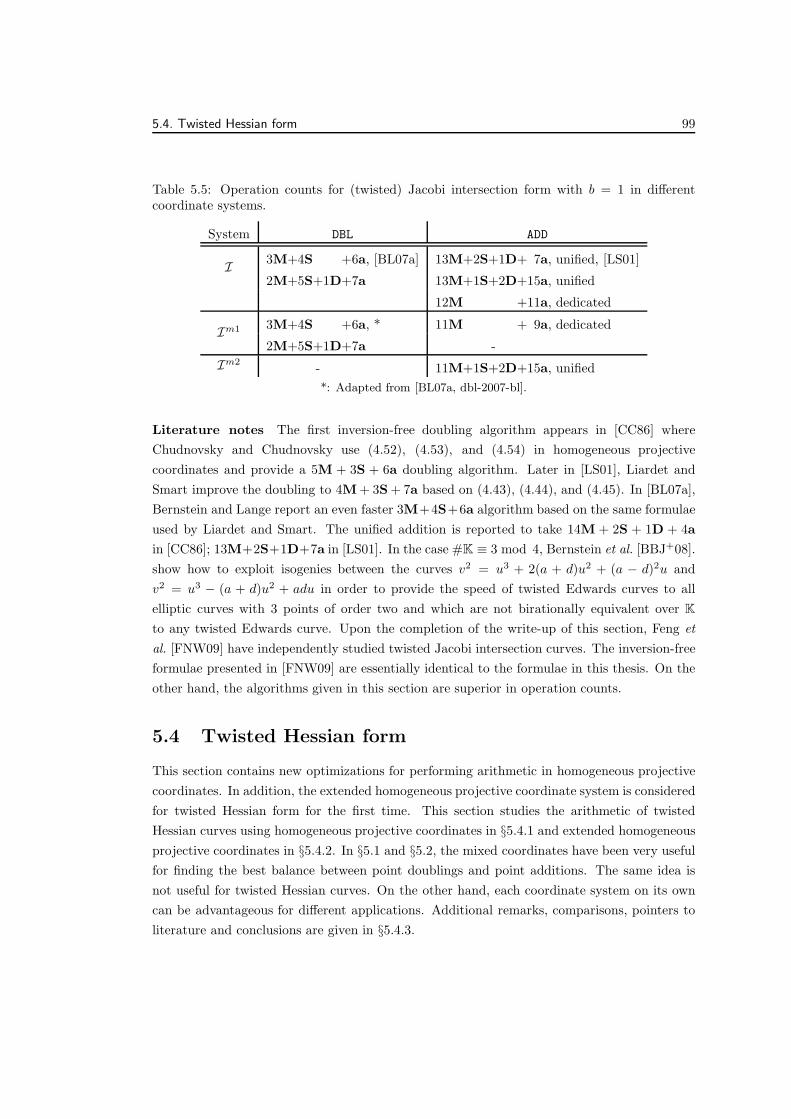
5.4. Twisted Hessian form 99
Table 5.5: Operation counts for (twisted) Jacobi intersection form with b = 1 in differentcoordinate systems.
System DBL ADD
I 3M+4S +6a, [BL07a] 13M+2S+1D+ 7a, unified, [LS01]
2M+5S+1D+7a 13M+1S+2D+15a, unified
12M +11a, dedicated
Im1 3M+4S +6a, * 11M + 9a, dedicated
2M+5S+1D+7a -
Im2- 11M+1S+2D+15a, unified
*: Adapted from [BL07a, dbl-2007-bl].
Literature notes The first inversion-free doubling algorithm appears in [CC86] where
Chudnovsky and Chudnovsky use (4.52), (4.53), and (4.54) in homogeneous projective
coordinates and provide a 5M + 3S + 6a doubling algorithm. Later in [LS01], Liardet and
Smart improve the doubling to 4M + 3S + 7a based on (4.43), (4.44), and (4.45). In [BL07a],
Bernstein and Lange report an even faster 3M+4S+6a algorithm based on the same formulae
used by Liardet and Smart. The unified addition is reported to take 14M + 2S + 1D + 4a
in [CC86]; 13M+2S+1D+7a in [LS01]. In the case #K ≡ 3 mod 4, Bernstein et al. [BBJ+08].
show how to exploit isogenies between the curves v2 = u3 + 2(a + d)u2 + (a − d)2u and
v2 = u3 − (a + d)u2 + adu in order to provide the speed of twisted Edwards curves to all
elliptic curves with 3 points of order two and which are not birationally equivalent over K
to any twisted Edwards curve. Upon the completion of the write-up of this section, Feng et
al. [FNW09] have independently studied twisted Jacobi intersection curves. The inversion-free
formulae presented in [FNW09] are essentially identical to the formulae in this thesis. On the
other hand, the algorithms given in this section are superior in operation counts.
5.4 Twisted Hessian form
This section contains new optimizations for performing arithmetic in homogeneous projective
coordinates. In addition, the extended homogeneous projective coordinate system is considered
for twisted Hessian form for the first time. This section studies the arithmetic of twisted
Hessian curves using homogeneous projective coordinates in §5.4.1 and extended homogeneous
projective coordinates in §5.4.2. In §5.1 and §5.2, the mixed coordinates have been very useful
for finding the best balance between point doublings and point additions. The same idea is
not useful for twisted Hessian curves. On the other hand, each coordinate system on its own
can be advantageous for different applications. Additional remarks, comparisons, pointers to
literature and conclusions are given in §5.4.3.

100 Chapter 5. Group law in projective coordinates
5.4.1 Homogeneous projective coordinates, HIn this system, each point (x, y) on ax3+y3+1 = dxy is represented with the triplet (X : Y : Z)
which corresponds to the affine point (X/Z, Y/Z) with Z 6= 0. These triplets satisfy the
homogeneous projective equation aX3+Y 3+Z3 = dXY Z. For all nonzero λ ∈ K, (X : Y : Z) =
(λX : λY : λZ). The identity element is represented by (0 : −1: 1). The negative of (X : Y : Z)
is (X : Z : Y ). This coordinate system is denoted by H throughout the text.
Doubling in H Let (X1 : Y1 : Z1) with Z1 6= 0 satisfy aX3 + Y 3 + Z3 = dXY Z. Then
[2](X1 : Y1 : Z1) = (X3 : Y3 : Z3) where
X3 = X1(Z31 − Y 3
1 ),
Y3 = Z1(Y31 − aX3
1 ),
Z3 = Y1(aX31 − Z3
1 ) (5.24)
assuming Z3 6= 0. These formulae are obtained from (4.25) and (4.26). It was pointed out
in [Ber06a] that Z3 is always nonzero if a is a non-cube in K. Also by Lemma 4.3.7, Z3 is
always nonzero if (X1 : Y1 : Z1) is of order r such that 3 ∤ r, regardless of the assumption on a
and d (of course, a(27a− d3) 6= 0).
These formulae do not depend on d. Therefore keeping d arbitrary has no effect on the cost
of (5.24). Evaluating (5.24) takes 6M + 3S + 1D + 3a in [BL07a];
A← X21 , B ← Y 2
1 , C ← Z21 , D← X1 ·A, E ← Y1 ·B, F ← Z1 · C,
G← aD, X3 ← X1 · (E − F ), Y3 ← Z1 · (G− E), Z3 ← Y1 · (F −G).
If a = 1 then the algorithm takes 6M + 3S + 3a. For this case, it is also possible to
exploit further optimizations. First of all, it is easy to see that X3 can be written as (X1Z1 −X1Y1)(Y
21 + Y1Z1 + Z2
1 ). If a = 1 then the same strategy also applies to Y3 and Z3. Based on
this observation it is possible to trade 3 multiplications with 3 squarings and several additions
if desired. The following 3M + 6S + 18a doubling algorithm exploits this idea;
A← X21 , B ← Y 2
1 , C ← Z21 , D ← A+B, E ← A+ C, F ← B +C,
G← ((X1 + Y1)2 −D)/2, H ← ((X1 + Z1)
2 − E)/2, J ← ((Y1 + Z1)2 − F )/2,
X3 ← (H −G) · (F + J), Y3 ← (J −H) · (D +G), Z3 ← (G− J) · (E +H).
Similar ideas apply to the case a = −1.
The previous doubling algorithms spend too much effort in squaring each of the input
coordinates. As an alternative optimization idea the following algorithm squares only Y1 and
takes 7M + 1S + 8a assuming that a = 1;
A← Y 21 , B ← (Z1 − Y1) · (A+ (Y1 + Z1) · Z1),
C ← (Y1 −X1) · (X1 · (X1 + Y1) +A), X3 ← X1 · B, Y3 ← Z1 · C,Z3 ← Y1 · (−B − C).
Similar ideas apply to the case a = −1.
For simplicity assume a = 1. So, D = 0. Note that the formulae do not depend on
d. The ratios S/M and a/M then determine the fastest of these three doubling algorithms.
The 3M + 6S + 15a algorithm is the fastest if a is very negligible and if S is cheaper than
M. Specifically, this algorithm takes over the 6M + 3S + 3a algorithm if M − S > 4a. The

5.4. Twisted Hessian form 101
7M + 1S + 8a algorithm takes over the 6M + 3S + 3a algorithm if 2S −M > 5a and takes
over the 3M+6S+15a algorithm if 4M− 5S < 7a. For instance, in an implementation where
S = 0.8M and a = 0.1M, these algorithms cost 8.7M, 9.3M, and 8.6M (in the respective
order the algorithms are introduced).
Dedicated addition in H Further let (X2 : Y2 : Z2) with Z2 6= 0 satisfy aX3 + Y 3 + Z3 =
dXY Z. Then, (X1 : Y1 : Z1) + (X2 : Y2 : Z2) = (X3 : Y3 : Z3) where
X3 = X21Y2Z2 − Y1Z1X
22 ,
Y3 = Z21X2Y2 −X1Y1Z
22 ,
Z3 = Y 21 X2Z2 −X1Z1Y
22 (5.25)
assuming Z3 6= 0. By Lemma 4.4.4, Z3 6= 0 if (X1 : Y1 : Z1) 6= (X2 : Y2 : Z2) and both summands
are of order r such that 3 ∤ r.
The addition law (5.25) is in fact the same law which was attributed to Cauchy and Sylvester
in [CC86]. The only difference is that the identity element is moved from a point at infinity to
(0 : − 1: 1) and remarkably (5.25) works for all twisted Hessian curves.
Evaluating (5.25) which is obtained from (4.29) and (4.30), takes 12M + 3a;
A← X1 · Z2, B ← Y1 · Z2, C ← Z1 ·X2, D ← Z1 · Y2, E ← X1 · Y2,
F ← Y1 ·X2, X3 ← A ·E − C · F, Y3 ← C ·D − A · B, Z3 ← B · F −D ·E.
Additionally, if Z2 = 1 then it takes 10M + 3a.
Alternatively, evaluating (5.25) takes 11M + 17a;
A← X1 · Z2, B ← Y1 · Z2, C ← Z1 ·X2, D ← Z1 · Y2, E ← X1 · Y2,
F ← Y1 ·X2, G← (C +E) · (A− F ), H ← (C − E) · (A+ F ),
J ← (C +B) · (A−D), K ← (C −B) · (A+D), X3 ← G−H, Y3 ← K − J,Z3 ← J +K −G−H − 2(E −B) · (F +D).
Here note that all coordinates are multiplied by 2. This algorithm is better than the
conventional 12M + 3a approach when 14a < 1M.
Unified addition in H Alternatively, (X1 : Y1 : Z1) + (X2 : Y2 : Z2) = (X3 : Y3 : Z3) where
X3 = X1Z1Z22 − Y 2
1 X2Y2,
Y3 = Y1Z1Y22 − aX2
1X2Z2,
Z3 = aX1Y1X22 − Z2
1Z2Y2 (5.26)
assuming Z3 6= 0. It was pointed out in [Ber06a] that Z3 6= 0 if a is a non-cube in K. Also by
Lemma 4.3.7, Z3 6= 0 if (X1 : Y1 : Z1) and (X2 : Y2 : Z2) are of order r such that 3 ∤ r.
Evaluating (5.26) which is obtained from (4.31) and (4.32), takes 12M+1D+3a in [BKL09];
A← X1 · Z2, B ← Z1 · Z2, C ← Y1 ·X2, D← Y1 · Y2, E ← Z1 · Y2,
F ← aX1 ·X2, X3 ← A · B − C ·D, Y3 ← D · E − F ·A, Z3 ← F · C −B ·E.
Additionally, if Z2 = 1 then it takes 10M + 1D + 3a.
Using the same optimization that removes a multiplication from the dedicated addition
algorithm, evaluating (5.26) takes 11M + 1D + 17a;
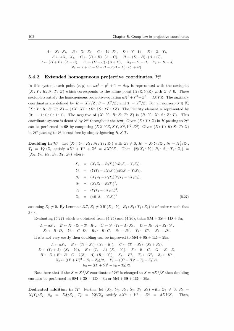
102 Chapter 5. Group law in projective coordinates
A← X1 · Z2, B ← Z1 · Z2, C ← Y1 ·X2, D ← Y1 · Y2, E ← Z1 · Y2,
F ← aX1 ·X2, G← (D +B) · (A− C), H ← (D −B) · (A+ C),
J ← (D + F ) · (A− E), K ← (D − F ) · (A+ E), X3 ← G−H, Y3 ← K − J,Z3 ← J +K −G−H − 2(B − F ) · (C +E).
5.4.2 Extended homogeneous projective coordinates, He
In this system, each point (x, y) on ax3 + y3 + 1 = dxy is represented with the sextuplet
(X : Y : R : S : T : Z) which corresponds to the affine point (X/Z, Y/Z) with Z 6= 0. These
sextuplets satisfy the homogeneous projective equation aX3+Y 3+Z3 = dXY Z. The auxiliary
coordinates are defined by R = XY/Z, S = X2/Z, and T = Y 2/Z. For all nonzero λ ∈ K,
(X : Y : R : S : T : Z) = (λX : λY : λR : λS : λT : λZ). The identity element is represented by
(0 : − 1: 0 : 0 : 1 : 1). The negative of (X : Y : R : S : T : Z) is (R : Y : X : S : Z : T ). This
coordinate system is denoted by He throughout the text. Given (X : Y : Z) in H passing to He
can be performed in 6S by computing (XZ, Y Z,XY,X2, Y 2, Z2). Given (X : Y : R : S : T : Z)
in He passing to H is cost-free by simply ignoring R,S, T .
Doubling in He Let (X1 : Y1 : R1 : S1 : T1 : Z1) with Z1 6= 0, R1 = X1Y1/Z1, S1 = X21/Z1,
T1 = Y 21 /Z1 satisfy aX3 + Y 3 + Z3 = dXY Z. Then, [2](X1 : Y1 : R1 : S1 : T1 : Z1) =
(X3 : Y3 : R3 : S3 : T3 : Z3) where
X3 = (X1Z1 −R1T1)(aR1S1 − Y1Z1),
Y3 = (Y1T1 − aX1S1)(aR1S1 − Y1Z1),
R3 = (X1Z1 −R1T1)(Y1T1 − aX1S1),
S3 = (X1Z1 −R1T1)2,
T3 = (Y1T1 − aX1S1)2,
Z3 = (aR1S1 − Y1Z1)2 (5.27)
assuming Z3 6= 0. By Lemma 4.3.7, Z3 6= 0 if (X1 : Y1 : R1 : S1 : T1 : Z1) is of order r such that
3 ∤ r.
Evaluating (5.27) which is obtained from (4.25) and (4.26), takes 9M + 3S + 1D + 3a;
A← aS1, B ← X1 · Z1 − T1 ·R1, C ← Y1 · T1 − A ·X1, D ← R1 · A− Z1 · Y1,
X3 ← B ·D, Y3 ← C ·D, R3 ← B · C, S3 ← B2, T3 ← C2, Z3 ← D2.
If a is not very costly then doubling can be improved to 5M + 6S + 1D + 29a;
A← aS1, B ← (T1 + Z1) · (X1 −R1), C ← (T1 − Z1) · (X1 +R1),
D← (T1 + A) · (X1 − Y1), E ← (T1 −A) · (X1 + Y1), F ← B − C, G← E −D,H ← D + E −B − C − 2(Z1 − A) · (R1 + Y1), S3 ← F 2, T3 ← G2, Z3 ← H2,
X3 ← ((F +H)2 − S3 − Z3)/2, Y3 ← ((G+H)2 − T3 − Z3)/2,
R3 ← ((F +G)2 − S3 − T3)/2.
Note here that if the S = X2/Z-coordinate of He is changed to S = aX2/Z then doubling
can also be performed in 9M + 3S + 1D + 3a or 5M + 6S + 1D + 29a.
Dedicated addition in He Further let (X2 : Y2 : R2 : S2 : T2 : Z2) with Z2 6= 0, R2 =
X2Y2/Z2, S2 = X22/Z2, T2 = Y 2
2 /Z2 satisfy aX3 + Y 3 + Z3 = dXY Z. Then,

5.4. Twisted Hessian form 103
(X1 : Y1 : R1 : S1 : T1 : Z1) + (X2 : Y2 : R2 : S2 : T2 : Z2) = (X3 : Y3 : R3 : S3 : T3 : Z3) where
X3 = (S1Y2 − Y1S2)(T1X2 −X1T2),
Y3 = (Z1R2 −R1Z2)(T1X2 −X1T2),
R3 = (S1Y2 − Y1S2)(Z1R2 −R1Z2),
S3 = (S1Y2 − Y1S2)2,
T3 = (Z1R2 −R1Z2)2,
Z3 = (T1X2 −X1T2)2 (5.28)
assuming Z3 6= 0. By Lemma 4.3.3, Z3 6= 0 if (X1 : Y1 : R1 : S1 : T1 : Z1) 6=(X2 : Y2 : R2 : S2 : T2 : Z2) and both summands are of order r such that 3 ∤ r.
Evaluating (5.28) which is obtained from (4.29) and (4.30), takes 9M + 3S + 3a;
A← S1 · Y2 − Y1 · S2, B ← Z1 ·R2 −R1 · Z2, C ← T1 ·X2 −X1 · T2, X3 ← A · C,Y3 ← B · C, R3 ← A ·B, S3 ← A2, T3 ← B2, Z3 ← C2.
Additionally, if Z2 = 1 then it takes 8M + 3S + 3a.
In addition, three multiplications can be traded with three squarings and several additions
if desired. The alternative evaluation takes 6M + 6S + 15a;
A← S1 · Y2 − Y1 · S2, B ← Z1 · R2 −R1 · Z2, C ← T1 ·X2 −X1 · T2, S3 ← A2,
T3 ← B2, Z3 ← C2, X3 ← ((A+ C)2 − S3 − Z3)/2,
Y3 ← ((B + C)2 − T3 − Z3)/2, R3 ← ((A+B)2 − S3 − T3)/2.
Additionally, if Z2 = 1 then it takes 5M + 6S + 15a.
Unified addition in He Alternatively, (X1 : Y1 : R1 : S1 : T1 : Z1) +
(X2 : Y2 : R2 : S2 : T2 : Z2) = (X3 : Y3 : R3 : S3 : T3 : Z3) where
X3 = (X1Z2 − T1R2)(aR1S2 − Z1Y2),
Y3 = (Y1T2 − aS1X2)(aR1S2 − Z1Y2),
R3 = (X1Z2 − T1R2)(Y1T2 − aS1X2),
S3 = (X1Z2 − T1R2)2,
T3 = (Y1T2 − aS1X2)2,
Z3 = (aR1S2 − Z1Y2)2 (5.29)
assuming Z3 6= 0. It can be deduced from [BBJ+08] that Z3 6= 0 if a is a square in K
and d is not a square in K. Also by Lemma 4.3.7, Z3 6= 0 if (X1 : Y1 : R1 : S1 : T1 : Z1) and
(X2 : Y2 : R2 : S2 : T2 : Z2) are of order r such that 3 ∤ r.
Evaluating (5.29) which is obtained from (4.31) and (4.32), takes 9M + 3S + 2D + 3a;
A← X1 · Z2 − T1 ·R2, B ← Y1 · T2 − aS1 ·X2, C ← aR1 · S2 − Z1 · Y2,
X3 ← A · C, Y3 ← B · C, R3 ← A ·B, S3 ← A2, T3 ← B2, Z3 ← C2.
Additionally, if Z2 = 1 then it takes 8M + 3S + 2D + 3a.
In addition, three multiplications can be traded with 3 squarings and several additions if
desired. The alternative evaluation takes 6M + 6S + 2D + 15a;

104 Chapter 5. Group law in projective coordinates
A← X1 · Z2 − T1 ·R2, B ← Y1 · T2 − aS1 ·X2, C ← aR1 · S2 − Z1 · Y2, S3 ← A2,
T3 ← B2, Z3 ← C2, X3 ← ((A+ C)2 − S3 − Z3)/2,
Y3 ← ((B + C)2 − T3 − Z3)/2, R3 ← ((A+B)2 − S3 − T3)/2.
Additionally, if Z2 = 1 then it takes 5M + 6S + 2D + 15a.
Note here that if the S = X2/Z-coordinate of He is changed to S = aX2/Z then the
unified addition naturally takes 9M + 3S + 1D + 3a or 6M + 6S + 1D + 15a eliminating one
multiplication by a.
5.4.3 Comparison and remarks
In 5.4.1, inversion-free arithmetic for twisted Hessian form is studied in homogeneous projective
coordinates, H. This subsection reviewed the previous results and has added new and
potentially more efficient results to the current body of knowledge. In particular, the proposed
unified addition algorithm takes 11M+ 1D+ 17a where an earlier algorithm in [BKL09] takes
12M + 1D + 3a. The new algorithm is faster when 1M > 14a. As well, dedicated addition
formulae are derived which eliminate multiplication by a. The proposed dedicated addition
algorithms take 12M + 3a and 11M + 17a. Moreover, in the case a = 1, it is shown that the
6M + 3S + 1D + 3a doubling algorithm in [BKL09] can be performed in 3M + 6S + 15a or
even 7M + 1S + 8a.
In §5.4.2, three additional coordinates are integrated into H. The new system is denoted
by He. In this system, it is shown that the additions can benefit from three M/S trade-offs
without any additional cost. In particular, the new unified addition takes 9M + 3S + 2D+ 3a
which can be further improved to 9M + 3S + 1D + 3a, see §5.4.2. This is an improvement
over the 12M + 1D + 3a algorithm in H. In the case a is practically negligible, a 6M + 6S +
1D + 15a unified addition algorithm is proposed. This algorithm is faster than the proposed
11M + 1D + 17a unified addition algorithm in H. Similar arguments apply to the proposed
dedicated addition.
Various operation counts in H and He are summarized in Table 5.6. Table 5.7 provides
operation counts for the case a = 1.
The determination of the optimum system and algorithms for Hessian form is very sensitive
to the changes in S/M, a/M and target applications.
Clearly, the doublings in He are quite inefficient in comparison to H and switching between
H and He is costly. Therefore, He is not suitable for speed oriented applications. On the
other hand, the unified addition in He for arbitrary non-cube a is still interesting if just unified
additions are being accessed, the cost of a and D are negligible, and S is much cheaper than M.
Other than these situations, H is better in performance. In addition, H needs three coordinates
rather than six. If 7M+1S+8a or 3M+6S+15a doubling algorithms in Table 5.7 are desired
for efficient implementation then parameter a should be rescaled to or selected as 1. In this
case, the completeness will always be lost. On the other hand, possible incorrect outputs can
be prevented by selecting the inputs from a suitable subgroup, see §5.4.1.
Literature notes The inversion-free arithmetic on Hessian curves x3+y3+1 = dxy was first
studied by Chudnovsky and Chudnosky [CC86] with the addition laws attributed to Cauchy

5.5. Short Weierstrass form 105
Table 5.6: Operation counts for twisted Hessian form in different coordinate systems.
System DBL ADD
H 6M+3S+1D+ 3a, [BKL09]
12M +1D+ 3a, unified, [BKL09]
11M +1D+17a, unified
12M + 3a, dedicated
11M +17a, dedicated
He
9M+3S+1D+ 3a9M+3S+2D+ 3a, unified
9M+3S + 3a, dedicated
5M+6S+1D+29a6M+6S+2D+15a, unified
6M+6S +15a, dedicated
Table 5.7: Operation counts for (twisted) Hessian form with a = 1 in different coordinatesystems.
System DBL ADD
H
6M+3S+ 3a, [BKL09] 12M + 3a, unified, [BKL09]
7M+1S+ 8a 11M +17a, unified
3M+6S+18a 12M + 3a, dedicated
11M +17a, dedicated
He
9M+3S+ 3a9M+3S+ 3a, unified
9M+3S+ 3a, dedicated
5M+6S+29a6M+6S+15a, unified
6M+6S+15a, dedicated
and Sylvester. Smart [Sma01] presented a 3-way parallel implementation of the dedicated
addition on the curve X3 + Y 3 + Z3 = dXY Z. Joye and Quisquater [JQ01] showed how to
use the dedicated addition formulae for point doubling by a permutation of coordinates and
suggested using these curves for side channel resistant applications. At that time addition
on Hessian curves was the fastest among all studied curve models. In all of these papers the
identity element is a point other than (0 : − 1: 1). In this section, [BKL09] was followed
in order to benefit from a simplified concept of complete additions on the twisted Hessian
curve aX3 + Y 3 + Z3 = dXY Z. Therefore, in all algorithms the identity element is moved to
(0 : − 1: 1).
5.5 Short Weierstrass form
In this section, short Weierstrass curves are reviewed with three coordinate systems. Most of
the results are directly taken from the literature for the completeness of the discussion. The
proposed improvements appear in unified addition.

106 Chapter 5. Group law in projective coordinates
5.5.1 Homogeneous projective coordinates, PIn this system, each point (x, y) on y2 = x3 + ax+ b is represented with the triplet (X : Y : Z)
which corresponds to the affine point (X/Z, Y/Z) with Z 6= 0. These triplets satisfy the
homogeneous projective equation Y 2Z = X3+aXZ2+bZ3. The identity element is represented
by (0 : 1 : 0). The negative of (X : Y : Z) is (X : −Y : Z). For all nonzero λ ∈ K, (X : Y : Z) =
(λX : λY : λZ). This coordinate system is denoted by P throughout the text.
Doubling in P Let (X1 : Y1 : Z1) with Z1 6= 0 satisfy Y 2Z = X3 + aXZ2 + bZ3. Then
[2](X1 : Y1 : Z1) = (X3 : Y3 : Z3) where
X3 = 2Y1Z1((3X21 + aZ2
1 )2 − 8Y 21 X1Z1),
Y3 = (3X21 + aZ2
1)(12Y 21 X1Z1 − (3X2
1 + aZ21 )2)− 8Y 4
1 Z21 ,
Z3 = 8Y 31 Z
31 (5.30)
assuming Z3 6= 0.
Evaluating (5.30) which is obtained from (4.1) and (4.2), takes 5M + 6S + 1D + 11a
in [BL07a, dbl-2007-bl];
A← 2Y1 · Z1, B ← Z21 , C ← X2
1 , D ← 4C + aB, E ← Y1 · A, F ← E2,
G← (X1 + E)2 − C − F, H ← D2 − 2G, X3 ← H ·A, Y3 ← D · (G−H)− 2F,
Z3 ← A ·A2.
If a = −3 then it takes 7M + 3S + 10a in [BL07a, dbl-2007-bl-2];
A← 3(X1 − Z1) · (X1 + Z1), B ← 2Y1 · Z1, C ← B2, D ← Y1 · B, E ← D2,
F ← 2X1 ·D, G← A2 − 2F, X3 ← B ·G, Y3 ← A · (F −G)− 2E, Z3 ← B · C.
Dedicated addition in P Further let (X2 : Y2 : Z2) with Z2 6= 0 satisfy Y 2Z = X3+aXZ2+
bZ3. Then, (X1 : Y1 : Z1) + (X2 : Y2 : Z2) = (X3 : Y3 : Z3) where
X3 = (X1Z2 − Z1X2)(Z1Z2(Y1Z2 − Z1Y2)2 − (X1Z2 + Z1X2)(X1Z2 − Z1X2)
2),
Y3 = (Y1Z2 − Z1Y2)((2X1Z2 + Z1X2)(X1Z2 − Z1X2)2 − Z1Z2(Y1Z2 − Z1Y2)
2)−Y1Z2(X1Z2 − Z1X2)
3,
Z3 = Z1Z2(X1Z2 − Z1X2)3 (5.31)
assuming Z3 6= 0.
Evaluating (5.31) which is obtained from (4.3) and (4.4), takes 12M+2S+7a in [CMO98];
A← Z1 · Z2, B ← X1 · Z2, C ← Y1 · Z2, D← B − Z1 ·X2, E ← C − Z1 · Y2,
F ← D2, G← D · F, H ← F ·B, J ← E2 · A+G− 2H, X3 ← D · J,Y3 ← E · (H − J)−G · C, Z3 ← A ·G.
Additionally, if Z2 = 1 then it takes 9M + 2S + 7a, see [CMO98].

5.5. Short Weierstrass form 107
Unified addition in P Alternatively, (X1 : Y1 : Z1) + (X2 : Y2 : Z2) = (X3 : Y3 : Z3) where
X3 = Z1Z2(Y1Z2 + Z1Y2)(2((X1Z2 + Z1X2)2 − Z1Z2(X1X2 − aZ1Z2))
2 −2Z1Z2(X1Z2 + Z1X2)(Y1Z2 + Z1Y2)
2),
Y3 = ((X1Z2 + Z1X2)2 − Z1Z2(X1X2 − aZ1Z2))(3Z1Z2(X1Z2 + Z1X2)(Y1Z2 + Z1Y2)
2 −2((X1Z2 + Z1X2)
2 − Z1Z2(X1X2 − aZ1Z2))2)− Z2
1Z22 (Y1Z2 + Z1Y2)
4,
Z3 = 2Z31Z
32 (Y1Z2 + Z1Y2)
3 (5.32)
assuming Z3 6= 0.
Evaluating (5.32) which is obtained from (4.5) and (4.6), takes 11M + 5S + 1D + 16a;
A← X1 ·X2, B ← Z1 · Z2, C ← (X1 + Z1) · (X2 + Z2)− A−B,D ← Y1 · Z2 + Z1 · Y2, E ← B ·D, F ← E ·D, G← C2, H ← F 2,
J ← G−B · (A− aB), K ← ((C + F )2 −G−H)/2, L← 2(J2 −K),
X3 ← E · L, Y3 ← J · (K − L)−H, Z3 ← 2E ·E2.
Additionally, if Z2 = 1 then it takes 9M + 5S + 1D + 16a.
5.5.2 Jacobian coordinates, JIn this system, each point (x, y) on y2 = x3 + ax+ b is represented with the triplet (X : Y : Z)
which corresponds to the affine point (X/Z2, Y/Z3) with Z 6= 0. These triplets satisfy the
weighted projective equation Y 2 = X3 + aXZ4 + bZ6. The identity element is represented by
(1 : 1 : 0). The negative of (X : Y : Z) is (X : − Y : Z). For all nonzero λ ∈ K, (X : Y : Z) =
(λ2X : λ3Y : λZ). This coordinate system is denoted by J throughout the text.
Doubling in J Let (X1 : Y1 : Z1) with Z1 6= 0 satisfy Y 2 = X3 + aXZ4 + bZ6. Then
[2](X1 : Y1 : Z1) = (X3 : Y3 : Z3) where
X3 = (3X21 + aZ4
1 )2 − 8X1Y21 ,
Y3 = (3X21 + aZ4
1 )(4X1Y21 −X3)− 8Y 4
1 ,
Z3 = 2Y1Z1 (5.33)
assuming Z3 6= 0.
Evaluating (5.33) which is obtained from (4.1) and (4.2), takes 1M + 8S + 1D + 14a
in [BL07a, dbl-2007-bl];
A← Z21 , B ← Y 2
1 , C ← X21 , D ← B2, E ← 2((X1 +B)2 − C −D),
F ← 3C + aA2, X3 ← F 2 − 2E, Y3 ← F · (E −X3)− 8D,
Z3 ← (Y1 + Z1)2 −B − A.
If a = −3 then it takes 3M + 5S + 12a in [BL07a, dbl-2001-b];
A← Z21 , B ← Y 2
1 , C ← X1 · B, D ← 3(X1 − A) · (X1 + A), X3 ← D2 − 8C,
Y3 ← D · (4C −X3)− 8B2, Z3 ← (Y1 + Z1)2 −B −A.

108 Chapter 5. Group law in projective coordinates
Dedicated addition in J Further let (X2 : Y2 : Z2) with Z2 6= 0 satisfy Y 2 = X3 +aXZ4 +
bZ6. Then, (X1 : Y1 : Z1) + (X2 : Y2 : Z2) = (X3 : Y3 : Z3) where
X3 = (Y1Z32 − Z3
1Y2)2 − (X1Z
22 + Z2
1X2)(X1Z22 − Z2
1X2)2,
Y3 = (Y1Z32 − Z3
1Y2)(Z21X2(X1Z
22 − Z2
1X2)2 −X3)− Z3
1Y2(X1Z22 − Z2
1X2)3,
Z3 = Z1Z2(X1Z22 − Z2
1X2) (5.34)
assuming Z3 6= 0.
Evaluating (5.34) which is obtained from (4.3) and (4.4), takes 11M+ 5S+ 11a in [BL07a,
add-2007-bl];
U2 ← Z22 , V2 ← U2 · Z2, U1 ← Z2
1 , V1 ← U1 · Z1, A← U1 ·X2, B ← V1 · Y2,
C ← X1 · U2 − A, D ← Y1 · V2 −B, E ← C2, F ← C ·E, G← A ·E,X3 ← D2 − F − 2G, Y3 ← D · (G−X3)−B · F,
Z3 ← C · ((Z1 + Z2)2 − U1 − U2)/2.
A 7M + 4S + 11a algorithm is provided in [BL07a, madd-2007-bl] for the case Z2 = 1.
Unified addition in J Alternatively, (X1 : Y1 : Z1) + (X2 : Y2 : Z2) = (X3 : Y3 : Z3) where
X3 = ((X1Z22 + Z2
1X2)2 − Z2
1Z22 (X1X2 − aZ2
1Z22 ))2 − (X1Z
22 + Z2
1X2)(Y1Z32 + Z3
1Y2)2,
Y3 =1
2(((X1Z
22 + Z2
1X2)2 − Z2
1Z22 (X1X2 − aZ2
1Z22 )) ·
((X1Z22 + Z2
1X2)(Y1Z32 + Z3
1Y2)2 − 2X3)− (Y1Z
32 + Z3
1Y2)4),
Z3 = Z1Z2(Y1Z32 + Z3
1Y2) (5.35)
assuming Z3 6= 0.
Evaluating (5.35) which is obtained from (4.5) and (4.6), takes 8M + 10S + 1D + 24a;
U2 ← Z22 , V2 ← U2 · Z2, U1 ← Z2
1 , V1 ← U1 · Z1, A← X1 ·X2,
B ← ((Z1 + Z2)2 − U1 − U2)/2, C ← B2, D ← (X1 + U1) · (X2 + U2)− A−C,
E ← Y1 · V2 + V1 · Y2, F ← E2, G← D2, H ← F 2, J ← G− C · (A− aC),
K ← ((F +D)2 −G−H)/2, X3 ← J2 −K, Y3 ← (J · (K − 2X3)−H)/2,
Z3 ← ((B + E)2 − C − F )/2.
Additionally, if Z2 = 1 then it takes 6M + 8S + 1D + 24a by deleteing B ← ((Z1 + Z2)2 −
U1 − U2)/2 and by replacing C ← B2 with C ← Z21 .
Chudnovsky Jacobian coordinates, J c This system was introduced by Chudnovsky and
Chudnovsky in [CC86]. In this system, each triplet in J is represented as (X : Y : Z : Z2 : Z3).
which saves time in additions however doublings are much slower. See [BL07b, §5] for further
explanations and simplification of the concept by using re-additions. Further details are omitted
here.
It is interesting to note that the proposed unified addition algorithm for Jacobian
coordinates takes only 7M + 9S + 1D + 24a in Chudnovsky Jacobian coordinates.
Modified Jacobian coordinates, Jm This system was introduced by Cohen et al. in
[CMO98]. In this system, each triplet in J is represented as (X : Y : Z : aZ4). This
5.5. Short Weierstrass form 109
representation saves time for arbitrary a in repeated doublings. On the other hand, the
performance is identical to J when a = −3. Therefore, further details are omitted here.
Mixed coordinates, J x Cohen et al. also suggest mixing different variants of Jacobian
coordinates to obtain the optimum performance. See [CMO98] for details.
5.5.3 Comparison and remarks
Short Weierstrass curves are the most studied curve model in cryptology. There are several
reasons for this:
• The short Weierstrass form, y2 = x3 + ax + b, covers all elliptic curves of large
characteristic.
• The proposal of ECC was made using the short Weierstrass form, see [Mil86] and [Kob87].
• Several standards recommend (some even enforce) the use of short Weierstrass form in
ECC applications.
• In affine coordinates, this form has the fastest point addition and point doubling formulae
to date.
• Mixed Jacobian coordinates had been the fastest system in carrying out inversion-
free point addition and point doubling for decades (ignoring the Montgomery ladder
algorithm). The situation, however, changed after a sequence of results between 2007
and 2009. See §5.1, §5.2, §5.3, §5.4 in this chapter for details.
In this section, the most efficient formulae are brought together. EFD [BL07a] also displays
all of these formulae. The contributions from this work appear in the case of unified addition.
Previously, unified additions were only considered in homogeneous project coordinates, P . In
particular, Brier/Joye unified addition algorithm proposed in [BJ02] takes 12M+5S+1D+10a.
Bernstein and Lange announced 11M + 6S + 1D + 15a variant of the same algorithm in
[BL07a]. The proposed unified addition algorithm in §5.5.1 takes 11M + 5S + 1D + 16a.
The new algorithm overtakes Brier/Joye algorithm when M > 6a and is always faster than
Bernstein/Lange algorithm.
Unified addition was never previously studied in Jacobian coordinates. In §5.5.1, a new
unified addition algorithm is proposed in J which takes 8M+10S+1D+24a. This algorithm
takes 7M+ 9S+ 1D+ 24a in Chudnovsky Jacobian coordinates. If the extra space for storing
Z2 and Z3 coordinates of Chudnovsky Jacobian coordinates is not an issue then the new unified
addition algorithm is faster than unified addition in homogeneous projective coordinates by
several M/S trade-offs.
Various operation counts including the present contributions are summarized in Table 5.8
and Table 5.9.
It is already concluded in many works that the optimum system is J x for arbitrary a in
speed implementations. In the case a = −3, it is better to stay in J and use re-additions which
correspond to addition timings in J c.

110 Chapter 5. Group law in projective coordinates
Table 5.8: Operation counts for short Weierstrass form in different coordinate systems.
System DBL ADD
P , [CC86] 5M+6S+1D+11a, [BL07a]
12M+ 5S+1D+10a, unified, [BJ02]
11M+ 6S+1D+15a, unified, [BL07a]
11M+ 5S+1D+16a, unified
12M+ 2S + 7a, dedicated, [CMO98]
J , [CC86]3M+6S+1D+ 9a, [HNM98]
8M+10S+1D+24a, unified
1M+8S+1D+14a, [BL07a]12M+ 4S + 7a, dedicated, [CMO98]
11M+ 5S +11a, dedicated, [BL07a]
J c, [CC86] 4M+6S+1D+ 4a, [CMO98]
7M+ 9S+1D+24a, unified
11M+ 3S + 7a, dedicated, [CMO98]
10M+ 4S +13a, dedicated, [BL07a]
Jm, [CMO98]4M+4S +10a, [CMO98] 12M+ 6S+1D+ 7a, dedicated, [CMO98]
3M+5S +13a, [BL07a] 11M+ 7S+1D+13a, dedicated, [BL07a]
J x, [CMO98]4M+4S +10a, [CMO98] 10M+ 5S+1D+ 7a, dedicated, *
3M+5S +13a, [BL07a] 8M+ 7S+1D+14a, dedicated, *
* Effective
Table 5.9: Operation counts for short Weierstrass form with a = −3 in different coordinatesystems.
System DBL ADD
P , [CC86] 7M+3S+10a, [BL07a]
12M+ 5S+1D+10a, unified, [BJ02]
11M+ 6S+1D+15a, unified, [BL07a]
11M+ 5S+1D+16a, unified
12M+ 2S + 7a, dedicated, [CMO98]
J , [CC86]4M+4S+ 9a, [HMV03]
8M+10S+1D+24a, unified
3M+5S+12a, [BL07a]12M+ 4S + 7a, dedicated, [CMO98]
11M+ 5S +11a, dedicated, [BL07a]
J c, [CC86] 4M+6S+ 4a, [CMO98]
7M+ 9S+1D+24a, unified
11M+ 3S + 7a, dedicated, [CMO98]
10M+ 4S +13a, dedicated, [BL07a]
Jm, [CMO98]4M+4S+10a, [CMO98] 12M+ 6S+1D+ 7a, dedicated, [CMO98]
3M+5S+13a, [BL07a] 11M+ 7S+1D+13a, dedicated, [BL07a]
J x, [CMO98]4M+4S+10a, [CMO98] 10M+ 5S+1D+ 7a, dedicated, *
3M+5S+13a, [BL07a] 8M+ 7S+1D+14a, dedicated, *
* Effective
If just unified additions are being accessed then the proposed algorithms are faster than
previous results in the literature. Selecting between P and J c depends on the S/M value. If
S < M then J c will be the optimum choice.

5.6. Conclusion 111
5.6 Conclusion
This chapter studied the inversion-free arithmetic in five forms of elliptic curves using
various point representations, alternative addition laws, and algorithms to obtain faster group
operations. In the literature, only dedicated addition laws were known for some forms while
only unified addition laws were known for some other forms. In this chapter, the gaps
are closed by equipping each form with low-degree dedicated addition formulae, low-degree
unified addition formulae, and low-degree doubling formulae. This chapter also reviewed many
addition laws from the literature. Each set of formulae was further investigated for the best
operations counts with optimized algorithms in various point representations. Moreover, this
chapter discussed practical ways of preventing incorrect summands when a particular law is
used, also see §4.6 of Chapter 4.
Bernstein et al.’s introduction of Edwards curves [BL07b] at Asiacrypt 2007 has focused a
lot of attention for efficient elliptic curve based implementations on Edwards form. In §5.1, the
speed of this form and its extended version twisted Edwards form is further improved in many
different ways. For instance, the proposed dedicated addition algorithm is shown to take less
effort for adding two distinct points, one of them given in homogeneous projective coordinates
and the other in affine coordinates. With the proposal of extended coordinates, dedicated
addition and unified addition are significantly sped up. The proposed mixed coordinate system
for twisted Edwards form allows the use of new faster additions together with the fast doubling
formulae by Bernstein et al. from [BBJ+08]. For technical details see §5.1.
In §5.2, the arithmetic of extended Jacobi quartic form is substantially improved. In
particular, the homogeneous projective coordinate system was shown to allow a very efficient
point doubling. The proposed optimizations in §5.1 also perfectly matched with this quartic
model. Exploiting the analogies between two quartic models, the speed of extended Jacobi
quartic form is brought quite close to the speed of twisted Edwards curves. Noting that
extended Jacobi quartic form covers all twisted Edwards curve plus all other curves of even
order, the arithmetic of extended Jacobi quartic form is still very interesting for many curves
which are not 1 or 2 isogenous to twisted Edwards curves. For technical details, see §5.2.
In §5.3 the speed of Jacobi intersection form has been improved for many D/M, S/M,
and a/M values. After proposed optimizations the speed of Jacobi intersection form has been
brought close to extended Jacobi quartic form. However, every Jacobi intersection form elliptic
curve is either 1 or 2 isogenous to a twisted Edwards curve, see [BBJ+08, §5]. Therefore, twisted
Edwards curves become more suitable representations for all elliptic curve which can be written
in Jacobi intersection form once the proposed improvements from §5.1 are applied.
In §5.4 the arithmetic of twisted Hessian curves has been improved for some a/M, D/M,
and S/M values which can be exploited in a wide range of applications. For instance, one
multiplication has been removed from both dedicated and unified addition algorithms at the
expense of some more additions in K. Note that in some implementations additions in K
are practically negligible. With the proposed improvements for some elliptic curves, (twisted)
Hessian form becomes a faster representation than short Weierstrass form.
A preliminary speed ranking between studied coordinate systems of elliptic curves is
discussed next where plausible suggestions are provided for implementations.

112 Chapter 5. Group law in projective coordinates
Operation count based comparison The easiest way to get a speed ranking is to find a
suitable elliptic curve for each form and compare operation counts for doubling and additions.
Table 5.10 provides selected operation counts in M for selected coordinate systems under the
assumptions D ≈ 0.1M, a ≈ 0.05M, and S = 0.8M. The columns are sorted in descending
order with respect to the column DBL.
Table 5.10: Operation counts in selected coordinate systems for each form.
System DBL reADD ADD ADD,Z2 = 1
H with a = 1 8.20M 11.85M 11.85M 9.85M
J x with a = −3 7.60M 13.75M 15.55M 10.75M
Ex with a = −1 6.50M 8.30M 8.50M 7.50M
I with b = 1 6.45M 12.55M 11.00M 10.55M
Qx with a = −1/2 6.35M 10.35M 10.55M 9.55M
Table 5.11 provides cost estimations per bit of the scalar for a variable single scalar
multiplication with variable base point. The columns are sorted in descending order with
respect to the column NEW, i.e. scalar multiplication cost in terms of M. For simplicity, the
total cost is calculated as 0.98×DBL+ 0.18×reADD. Although this is a rough estimation, the
ranking between the systems does not change for a majority of plausible assumptions on the
cost of S, D, and a. For a more detailed cost analysis see [BL08].
Table 5.11: Cost estimate of SMUL per bit of scalar in M.
System OLD NEW
Twisted Hessian form, H with a = 1 10.58M 10.17M
Short Weierstrass form, J x with a = −3 9.92M -
Jacobi intersection form, I with a = 1 9.01M 8.43M
Extended Jacobi quartic form, Qx with a = −1/2 10.00M 8.07M
Twisted Edwards form, Ex with a = −1 8.31M 7.87M
This table highly benefits from the algorithms proposed in this chapter. For instance, if the
system Qw were considered for extended Jacobi quartic form with d = 1 using the doubling
and re-addition algorithms in [BL07a, dbl-2007-bl] then the cost estimation would have been
10.00M per bit after several cached values. This would put Qw even behind J with a = −3.
Similarly, if the system E were used for twisted Edwards form as in [BBJ+08] then the cost
estimation for twisted Edwards form with a = 1 would be 8.40M per bit. If the system E i were
used for twisted Edwards form as in [BBJ+08] then the cost estimation for twisted Edwards
form with a = 1 would be 8.31M per bit. Similarly, if the system H is used for twisted Hessian
form as described in [BKL09] then the cost estimation for twisted Hessian form with some
extremely small non-cube a would be 10.58M per bit. Similarly, if the system I is used for
Jacobi intersection form as described in [LS01] then the cost estimation for Jacobi intersection
form with some extremely small non-cube a would be 9.01M per bit.

5.6. Conclusion 113
An implementation based ranking will be provided later in Chapter 6 where the results of
this chapter are supported by experiments.
Curve based comparison This discussion gives a fairly satisfying idea of the speed ranking
between different forms when a suitable elliptic curve is selected for each form. On the other
hand, such a discussion leads to comparing speeds of elliptic curves which are possibly not
isomorphic (or not birational) or not isogenous. From an cryptographic point of view this is no
problem since over a large field, finding a suitable curve which resists attacks of concern (and
which has small curve constants if desired), is enough to satisfy the cryptographic interest.
From a mathematical point of view, however, it is better to determine the fastest form for a
fixed elliptic curve. The discussion is now focused on this aspect.
First of all, short Weierstrass form is always a fallback model for fairly efficient
implementation because any elliptic curve (of large characteristic) can be represented on the
curve EW,a4,a6, see Chapter 2. For arbitrary a4, the optimum system is the mixed coordinates
J x introduced by Cohen et al. in [CMO98] which is further discussed and improved in [BL08].
If a = −3 then J is the optimum system with cached Z2 for dedicated additions.
Now, fix an elliptic curve E of order r such that 2 | r. Then, the elliptic curve is isomorphic
(over the same field) to a Weierstrass curve y2 = x(x2 + a′2x + a′4) which is birationally
equivalent (over the same field) to the extended Jacobi quartic form elliptic curve given by
EQ,−a′
2/4,(a′2
2−4a′
4)/16, see §2.3 of Chapter 2. It is suitable here to note that every extended
Jacobi quartic curve EQ,d,a is birationally equivalent (over the same field) to a Weierstrass
curve given by y2 = x(x2 − 4ax + 4a2 − 4d). Performing the arithmetic on this curve in
extended Jacobi quartic form is always faster than performing the analogous operations on the
corresponding short Weierstrass form because even for arbitrary a and d both point doublings
and point additions in Qx are faster than in J with a4 = −3, (the fastest case in short
Weierstrass). In particular, doubling in Qx takes 2M + 5S + 1D + 7a where doubling in Jwith a4 = −3 takes 3M + 5S + 12a. But, even if D = M point doubling in Qx is still faster.
Similarly, a dedicated point addition in Qx takes an effective 6M + 4S + 3D + 17a where the
fastest dedicated point addition in J c with a4 = −3 takes 10M+4S+13a. So, even if D = M
point addition in Qx is still faster. In conclusion, for elliptic curves of even order extended
Jacobi quartic form becomes the new fallback curve model.
Now, further assume that 4 | r. Then, the curve is either 1 or 2 isogenous to a twisted
Edwards curve. Performing the arithmetic on this curve in twisted Edwards form is always
faster than performing the analogous operations in the corresponding short Weierstrass form.
In particular, a dedicated point addition in Ex takes an effective 9M+1D+7a where the fastest
dedicated point re-addition in J c with a4 = −3 takes 10M + 4S + 13a. So, even if D = M
point addition in Ex is faster by more than 4S. Point doubling in Ex takes 3M+4S+1D+6a
where doubling in J with a = −3 takes 3M + 5S + 12a. It is ideal to rescale the constant a
of a twisted curve to −1 for maximum performance. This requires −a to be a square in the
underlying field. Even if this is not possible it is always possible to rescale a to a very small
constant. So, it makes sense to assume D < S. So, even if D = S point doubling in Ex is
faster than point doubling in J with a4 = −3. In conclusion, for elliptic curves whose order
is divisible by four, twisted Edwards form becomes a fallback curve model (using an isogenous

114 Chapter 5. Group law in projective coordinates
curve if necessary).
Since every twisted Edwards curve is isomorphic (over the same field) to an extended Jacobi
quartic curve, it is also reasonable to make a speed comparison between these two models. An
investigation of the worst case scenario for the twisted Edwards form is done first. The curve
parameter a of the twisted Edwards curve can always be rescaled to a very small value so that
D ≤ a and consequently a dedicated point addition in Ex takes at most an effective 9M + 8a.
In the best case a dedicated addition in Qx will take an effective 6M+ 4S + 17a which can be
faster than point addition in Ex for which the worst case rules apply. Plus, point doubling inQx
is always faster than point doubling in Ex for the worst case scenario for the twisted Edwards
curve. Therefore, for some twisted Edwards curves, the corresponding extended Jacobi quartic
curve can be faster. Now, the worst case scenario for the extended Jacobi quartic form is
investigated. Since 4 | r the extended Jacobi quartic curve is 1 or 2 isogenous to a twisted
Edwards curve. The curve parameter a of the extended Jacobi quartic can always be rescaled
to a very small value so that D ≤ a and consequently a dedicated point addition in Qx takes
at most an effective 6M+4S+2D+17a. In the best case a dedicated addition in Ex will take
an effective 8M + 10a which is always faster than point addition in Qx for which the worst
case rules apply. Point doubling in Qx takes 2M + 5S + 7a in the worst case which can only
be as fast as point doubling in Ex if M = S. Therefore, keeping in mind the assumption 4 | r,for some extended Jacobi quartic curves, the corresponding 1 or 2 isogenous twisted Edwards
curve can be faster. In conclusion, extended Jacobi quartic curves and twisted Edwards curves
are not fallback curve models for each other in every situation.
Every Jacobi intersection curve is 1 or 2 isogenous to a twisted Edwards curve. After a
suitable rescaling of constants, it is easy to conclude after similar discussions that twisted
Edwards form is a faster alternative to Jacobi intersection form.
Now, assume that 3 | r but 6 ∤ r. Such curves can be written in Weierstrass form or twisted
Hessian form. It is easy to conclude after similar discussions that twisted Hessian form and
short Weierstrass form are not fallback curve models for each other in every situation. On the
other hand, if 6 | r then both extended Jacobi quartic form and twisted Edwards form become
faster for such elliptic curves.

Chapter 6
Experimental results
This chapter provides details on the implementation of elliptic curve scalar multiplication in the
light of new results from this work. The aim is to show that ECC applications can practically
benefit from the proposed algorithms. To achieve this aim, one has to face an enormous number
of design choices. These choices are investigated by categorizing different components of the
implementation as follows:
- hardware,
- finite field and its construction,
- elliptic curve, its representation, doubling and addition algorithms,
- scalar multiplication algorithm
where each item has intrinsic interactions with the others. These interactions are briefly
explained in the following sections. In particular, §6.1 is about the preferred programming
languages and the hardware where the scalar multiplications are computed. §6.2 contains
details about how the finite field arithmetic is developed. §6.3 makes an overview of best
operation counts for each of the five forms studied in this thesis. §6.4 presents experimental
results of the implemented scalar multiplication algorithms. The conclusions of this chapter
are drawn and final remarks are provided in §6.5.
6.1 Hardware and programming environment
Features and restrictions of hardware influence strongly the code to be designed. Some
hardware is so restricted that the programmer has to keep the compiled-code size to a minimum.
Smart Cards and wireless sensor network gadgets are examples of this kind. On such hardware,
the built-in word size tends to be small. Therefore inlining or loop-unrolling techniques are
most likely to generate a large compiled-code. In addition, only very small lookup tables
are practical. On the other hand, contemporary desktop processors come with large and fast
115

116 Chapter 6. Experimental results
internal cache memories, multi-level pipelining mechanisms, specialized SIMD instruction sets
and the like. This time the programmer’s challenge is to eliminate branches and minimize
the memory access by wisely using the internal registers and the available cache. Yet in some
other cases (such as military applications) it is important to hide the side channel information
leakage. As a consequence of these, the ratios I/M, S/M, D/M, and a/M are affected by the
way the underlying field arithmetic is implemented.
Due to ease of access, the experiments in this chapter are optimized for a desktop processor:
a single core of an 64-bit Intel Core 2 Duo (E6550) processor. The finite field layer of the
code is time-critical. Therefore, an assembly optimized finite field layer is an indispensable
component of the implementation. This layer was written in assembly language using the
x86-64 instruction set excluding the SIMD instructions. All higher level operations were
written in plain C language. For efficiency purposes, dynamic memory allocations were
prevented. Therefore, the stack was used to store all points, look-up tables, etc. The code was
compiled with the GCC compiler (the -O2 flag set). The executables were run on an Ubuntu 9
platform.
6.2 Finite field arithmetic
The implementation of finite field arithmetic is a crucial step in developing efficient ECC
applications. Although this thesis does not concentrate on improving finite field arithmetic, an
optimized finite field layer is needed in order to test the performance of the proposed algorithms.
Every finite field L contains (up to isomorphism) a unique subfield K ∼= Z/pZ. In the
case where p is large, it is reasonable to implement the arithmetic of K using multiprecision
integers since p typically does not fit into a single computer word. See [HMV03, §2.2] and
[CF05, §10,§11] for details. With modular integer arithmetic, the field operations in K such
as addition, multiplication, and inversion, can be built up. See [BZ09] for details on modular
and multiprecision arithmetic. If L = K then there is nothing more to do. If L ⊃ K then an
efficient field towering technique can be adapted to perform operations in L. For mathematical
details of field constructions see [LN96]. For efficiency related discussions see [BS09]. The
simplest and the most efficient finite field implementations have L = K and p of extremely low
or extremely high Hamming weight. Selecting p in this fashion, however, is not always possible.
For instance, the latest techniques for generating pairing friendly elliptic curves often yield an
arbitrary p. For arbitrary p, one of the best methods to follow is Montgomery’s n-residue
arithmetic, see [Mon85].
The code is designed to serve for other prime fields with characteristic p of the form p =
2256 − c where c is a suitable positive integer with at most 64-bits. On a 64-bit processor
each field element fits into only 4 computer words. Consequently, the assembly codes for basic
field operations such as addition and multiplication are not very long. However, accurately
measuring the cycle counts of each operation is practically hard due to high levels of the
pipelining in a Core 2 processor. Each of these operations is partially overlapped in the
execution by the preceding and the following operations. Plus compiler optimizations can
change the position and the number of instructions. As a rough but consistent way of estimating
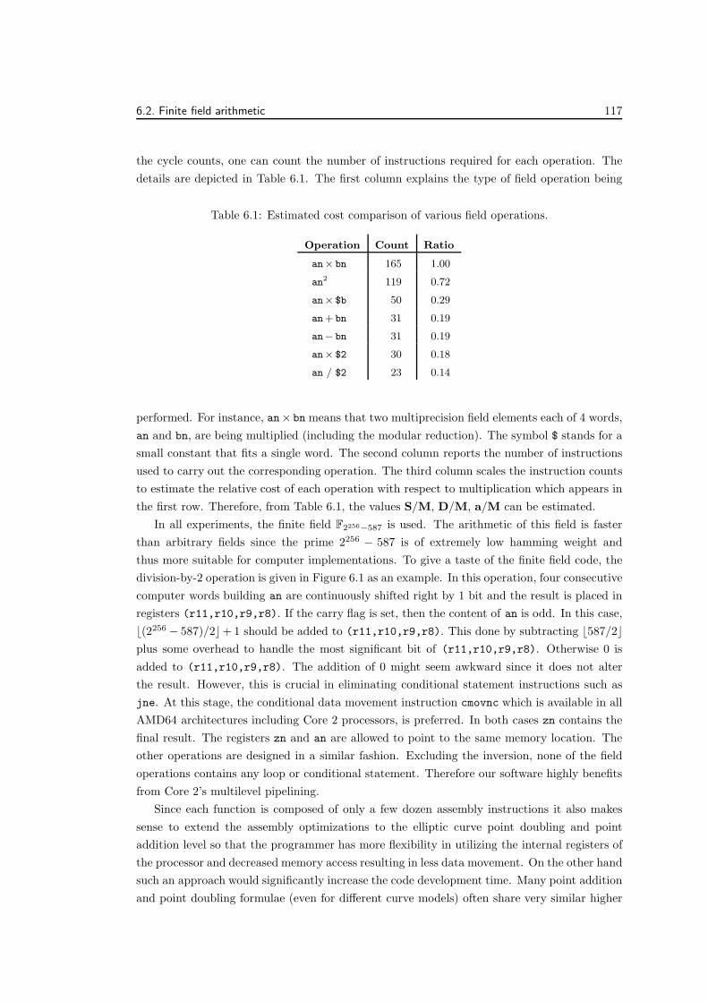
6.2. Finite field arithmetic 117
the cycle counts, one can count the number of instructions required for each operation. The
details are depicted in Table 6.1. The first column explains the type of field operation being
Table 6.1: Estimated cost comparison of various field operations.
Operation Count Ratio
an× bn 165 1.00
an2 119 0.72
an× $b 50 0.29
an+ bn 31 0.19
an− bn 31 0.19
an× $2 30 0.18
an / $2 23 0.14
performed. For instance, an× bn means that two multiprecision field elements each of 4 words,
an and bn, are being multiplied (including the modular reduction). The symbol $ stands for a
small constant that fits a single word. The second column reports the number of instructions
used to carry out the corresponding operation. The third column scales the instruction counts
to estimate the relative cost of each operation with respect to multiplication which appears in
the first row. Therefore, from Table 6.1, the values S/M, D/M, a/M can be estimated.
In all experiments, the finite field F2256−587 is used. The arithmetic of this field is faster
than arbitrary fields since the prime 2256 − 587 is of extremely low hamming weight and
thus more suitable for computer implementations. To give a taste of the finite field code, the
division-by-2 operation is given in Figure 6.1 as an example. In this operation, four consecutive
computer words building an are continuously shifted right by 1 bit and the result is placed in
registers (r11,r10,r9,r8). If the carry flag is set, then the content of an is odd. In this case,
⌊(2256 − 587)/2⌋+ 1 should be added to (r11,r10,r9,r8). This done by subtracting ⌊587/2⌋plus some overhead to handle the most significant bit of (r11,r10,r9,r8). Otherwise 0 is
added to (r11,r10,r9,r8). The addition of 0 might seem awkward since it does not alter
the result. However, this is crucial in eliminating conditional statement instructions such as
jne. At this stage, the conditional data movement instruction cmovnc which is available in all
AMD64 architectures including Core 2 processors, is preferred. In both cases zn contains the
final result. The registers zn and an are allowed to point to the same memory location. The
other operations are designed in a similar fashion. Excluding the inversion, none of the field
operations contains any loop or conditional statement. Therefore our software highly benefits
from Core 2’s multilevel pipelining.
Since each function is composed of only a few dozen assembly instructions it also makes
sense to extend the assembly optimizations to the elliptic curve point doubling and point
addition level so that the programmer has more flexibility in utilizing the internal registers of
the processor and decreased memory access resulting in less data movement. On the other hand
such an approach would significantly increase the code development time. Many point addition
and point doubling formulae (even for different curve models) often share very similar higher

118 Chapter 6. Experimental results
static INLINE void dv2(unsigned long *zn, unsigned long *an)
__asm__ VOLATILE (
"movq %2,%%rax; movq 8*3(%%rax),%%r11; shrq $0x1,%%r11; movq 8*2(%%rax),%%r10;
rcrq $0x1,%%r10; movq 8*1(%%rax),%%r9; rcrq $0x1,%%r9; movq 8*0(%%rax),%%r8;
rcrq $0x1,%%r8; movq %1,%%rax; movq %0,%%r12; movq $0x0,%%rdx; cmovnc %%rdx,%%r12;
movq $0x8000000000000000,%%rbx; cmovnc %%rdx,%%rbx; subq %%r12,%%r8;
movq %%r8,8*0(%%rax); sbbq $0x0,%%r9; movq %%r9,8*1(%%rax); sbbq $0x0,%%r10;
movq %%r10,8*2(%%rax); sbbq %%rbx,%%r11; movq %%r11,8*3(%%rax);"
: : "n" (587>>1), "m" (zn), "m" (an)
: "%rax", "%rbx", "%rdx", "%r8", "%r9", "%r10", "%r11", "%r12", "memory"
);
Figure 6.1: Sample F2256−587 operation: Divide-by-2 with no conditional statement.
level operations e.g. (an± bn)2, (an± bn)2-an2-bn2, an× bn± cn and an× bn± cn× dn.
These operations when implemented properly can eliminate several instructions resulting in a
slight speed-up. Therefore, it would be of interest implementing these additional functions as
a future study.
6.3 Elliptic curve operations
The tools of Chapter 3 have led to a discovery of many new affine formulae which are presented
together with the existing results in Chapter 4. In Chapter 5, several coordinate systems are
reviewed/studied to find the best operation counts. In this section, the aim is to determine
the best choice of those coordinate systems and algorithms that facilitate the fastest scalar
multiplication on suitable elliptic curves.
Selecting the curve In the experiments, five curves are used. Each curve is selected in a
way to contain a large prime order subgroup. The curve constants are small enough to fit
a computer word so that multiplication with curve constants can be performed faster than
a general multiplication. Table 6.2 shows the selected curves. The first column specifies the
elliptic curve. The second shows the co-factor of the curve.
Table 6.2: Sample elliptic curves over F2256−587.
Curve Equation h
Short Weierstrass, ES y2 = x3 − 3x+ 2582 1
Extended Jacobi quartic, EQ y2 = 25629x4 − x2 + 1 2
(Twisted) Hessian, EH x3 + y3 + 1 = 53010xy 3
Twisted Edwards, EE −x2 + y2 = 1 + 3763x2y2 4
(Twisted) Jacobi intersection, EI s2 + c2 = 1, 3764s2 + d2 = 1 4
The curves in the last two entries are birationally equivalent. For the convenience of the
reader, the number of points on each of the sample curves are given in the respective order as
they appear in Table 6.2 as follows expressed as a product of prime powers:

6.3. Elliptic curve operations 119
115792089237316195423570985008687907852860720292049485254475170270783237989437,
2x57896044618658097711785492504343953926355150900196614082809808174325972796687,
3x38597363079105398474523661669562635951141196656339482509250363382136009746847,
4x28948022309329048855892746252171976963455976009569136404907647803823651929949,
4x28948022309329048855892746252171976963455976009569136404907647803823651929949.
All of these curves can resist all known attacks which are summarized in Appendix B.
These curves are of negative trace and the number of points on each curve has fewer bits than
256. Therefore, any scalar (modulo the group order) also fits into a 256-bit string.
Selecting the coordinate system Finding the most efficient coordinate system depends
on several factors. The values I/M, S/M, D/M, a/M affect how the most efficient point
doubling and addition algorithms are determined. The frequency of point doubling and
addition operations affect how the most efficient coordinate system is determined. To simplify
this process, Table 6.3 provides a summary of operation counts for the most frequently accessed
operations in scalar multiplication. This table contains only the selected coordinate systems
and selected operation counts. For more alternatives and comparisons see Chapter 5.
Table 6.3: Selected operation counts for the most frequently accessed operations.
Curve Cond. Coordinate System DBL reADD
ShortWeierstrass
a = −1 P , (X : Y : Z) 7M + 3S 12M + 2S
a = −3 J , (X : Y : Z) 3M + 5S 10M + 4S
(Twisted)Hessian
a = 1 H, (X : Y : Z)7M + 1S or
11M3M + 6S
(Twisted)Jacobiintersection
b = 1 Im1, (S : C : D : Z : U : V )3M + 4S or
11M2M + 5S + 1D
ExtendedJacobiquartic
d = 1 Qw, (X : Y : Z) 2M + 6S + 1D 10M + 3S + 1D
a = −1/2 Q, (X : Y : Z) 2M + 5S 10M + 5S + 2D
a = −1/2 Qe, (X : Y : T : Z) 8S 7M + 3S + 2D
a = −1/2 Qx 2M + 5S 6M + 4S + 2D*
TwistedEdwards
a = −1 E , (X : Y : Z) 3M + 4S 10M + 1S + 1D
a = −1 E i, (X : Y : Z) 3M + 4S + 1D 9M + 1S + 1D
a = −1 Ee, (X : Y : T : Z) 4M + 4S 8M
a = −1 Ex 3M + 4S 8M*
*Effective, see §5.2.3 and §5.1.4 in Chapter 5.
In Table 6.3, two systems are more efficient than the other entries in terms of operation
counts regardless of S/M, D/M, a/M values or the frequencies of doublings and additions.
These systems are Qx and Ex; both are outcomes of this thesis. In the experiments, Qx is
used for the extended Jacobi quartic curve y2 = 25629x4 − x2 + 1 and Ex is used for the
twisted Edwards curve −x2 + y2 = 1 + 3763x2y2. For the twisted Hessian curve x3 + y3 +
1 = 53010xy, the coordinate system H is used. Similarly, for the Jacobi intersection curve
s2 + c2 = 1, 3764s2 + d2 = 1, the coordinate system Im1 is used. For the Weierstrass curve

120 Chapter 6. Experimental results
y2 = x3−3x+2582 Jacobian coordinate system J is known to be more efficient than projective
coordinate system P . Therefore, Jacobian coordinates are used for the Weierstrass curve.
6.4 Scalar multiplication
The highest level task is to put the pieces of a scalar multiplication together. As in lower
level operations, there are so many design issues such as the selection of a scalar recoding
algorithm, powering algorithm, determining the optimal size of lookup tables, the elimination of
unnecessary conditional statements, etc. Studying all possible scenarios would only complicate
the experiments without changing most conclusions that can be derived from the results. To
keep design alternatives to a minimum, two experiments are conducted. These experiments
involve single-variable-point-single-variable-scalar multiplication and single-fixed-point-single-
variable-scalar multiplication which are presented in §6.4.1 and §6.4.2, respectively.
6.4.1 Experiment1: Scalar multiplication with variable base-point
This section provides implementation timings for elliptic curve single-variable-point-single-
variable-scalar multiplication. Algorithm 3.38 in [HMV03] is implemented for this pupose. As
for the integer recoding part of the scalar multiplication, w-LtoR algorithm in [Ava05] is used.
This part of the implementation runs on-the-fly as the main loop of the scalar multiplication
is performed. The scalar multiplication algorithm starts with building a look-up table. To
accommodate this computation 3P, 5P, . . . , 15P are precomputed by the sequence of operations
2P, 2P + P, 2P + 3P, . . . , 2P + 13P . In this implementation I/M ≈ 121. Therefore, the
precomputed values are not normalized (i.e. conversion to affine form) following the analysis
in [BL08]. Also following the same reference, double-and-add algorithms with Z = 1 are
also used to obtain speed-ups of the scalar multiplication. Table 6.4 summarizes measured
average clock cycles for a single-variable-point-single-variable-scalar multiplication on different
representations of elliptic curves. The reverse-order of the entries in Table 6.4 was used to sort
the main sections of Chapter 5.
Table 6.4: Cycle-counts (rounded to the nearest one thousand) for 256-bit scalar multiplicationwith variable base-point
Curve & coordinate system w Approximate operation counts Cycles
Short Weierstrass (a = −3), J x 5 I+1598M+1156S+ 0D+2896a 468,000
(Twisted) Hessian (a = 1), H 5 I+2093M+ 757S+ 0D+1177a 447,000
(Twisted) Jacobi intersection (b = 1), Im1 5 I+1295M+1011S+ 0D+2009a 383,000
Extended Jacobi quartic (a = −1/2), Qx 5 I+1162M+1110S+102D+1796a 376,000
Twisted Edwards (a = −1), Ex 6 I+1202M+ 969S+ 0D+2025a 362,000
The implementation is developed only for the most efficient formulae for each form. For
instance, weighted projective Jacobi quartic coordinates or homogeneous projective twisted
Edwards coordinates are not implemented in these experiments. Therefore, the comparisons
are made relative to the Jacobian coordinates.

6.4. Scalar multiplication 121
For J x, a 4M + 4S point doubling algorithm is used from [HMV03], also see [BL07a, dbl-
2004-hmv]. As for the additions, a 12M+4S algorithm from [CMO98] is used. For readditions
this algorithm needs 11M + 3S. The M/S trade-offs in Table 6.3 are not helpful for this
implementation. The situation may be different in other implementations. For H, only the
classic algorithms are implemented. The proposed algorithms in this thesis are slightly slower
in this implementation because a is not negligible. On the other hand, other implementations
may still benefit from the proposed algorithms. For Im1, the 3M + 4S doubling algorithm
is preferred, see [BL07a, dbl-2007-bl]. Point additions are implemented as proposed in this
thesis, see Table 6.3 and §5.3.2 of Chapter 5. For Qx and Ex, the operation counts from
Table 6.3 apply except for a few M/S trade-offs which are not used in order to limit the
number of a’s.
Using several coordinates to represent points might raise the belief that there will be a
significant overhead of handling extra coordinates. It was empirically observed that these
overheads are negligible. If they were non-negligible then there would be a speed problem with
twisted Jacobi intersection implementation. In fact, once the field operations are removed,
the remaining code including the integer recoding part of the scalar multiplication takes less
than 3% of the execution time. With the integer recoding excluded, it takes less than 1%
of the execution time. Furthermore, the extra coordinates also serve as local variables when
performing point doubling and point additions. Therefore, having more than 3 coordinates
does not constitute an efficiency issue in the case of modern desktop processors. If the scalar
multiplication needs fewer field multiplications with the extra coordinates then it is always
worth using the extended coordinate systems.
6.4.2 Experiment2: Scalar multiplication with fixed base-point
In the case where the base-point is fixed the timings can be dramatically improved by using
Algorithm 3.44 or Algorithm 3.45 in [HMV03]. These algorithms are reported to be special
cases of the exponentiation techniques in [LL94]. Both algorithms are point addition intensive,
i.e. the point doublings are less important in overall efficiency.
So far the most efficient point addition algorithm among existing point addition algorithms1
is an outcome of this thesis. This algorithm requires only 8M for each point addition on
a twisted Edwards curve. It is reasonable to implement Algorithm 3.45 in [HMV03] by
incorporating this new algorithm and compare it to the efficiency of J .
Table 6.5 provides measured cycles on Core 2. The first column specifies the coordinate
system. The second column is the window length w of the Algorithm 3.45 in [HMV03]. This
algorithm uses two look-up tables by default. Within this implementation, this was generalized
to an arbitrary number of tables. The third column s tells how many look-up tables are used.
For instance, w = 8 and s = 4 means that s × 2w = 4 × 28 = 1024 precomputed points are
stored in look-up tables. Each coordinate fits into 32 bytes. So, an affine point (x, y) needs 64
bytes. Therefore, the look-up tables take 64 KB (kilobyte). The space consumption is reflected
in the fourth column. The fifth column contains the averaged cycle counts on a single core of
Core 2.
1Excluding differential point additions.

122 Chapter 6. Experimental results
Table 6.5: Cycle-counts (rounded to the nearest one thousand) for 256-bit scalar multiplicationwith fixed base-point
Curve & coordinate system w s Look-up Cycles
Short Weierstrass (a = −3), J
4 4 2 KB× 2 138,000
8 1 8 KB× 2 121,000
8 2 16 KB× 2 102,000
8 4 32 KB× 2 92,000
8 8 64 KB× 2 86,000
Twisted Edwards (a = −1), Ex,precomputed t
4 4 2 KB× 3 131,000
8 1 8 KB× 3 115,000
8 2 16 KB× 3 96,000
8 4 32 KB× 3 87,000
8 8 64 KB× 3 79,000
Twisted Edwards (a = −1), Ee,precomputed t
4 4 2 KB× 3 122,000
8 1 8 KB× 3 107,000
8 2 16 KB× 3 90,000
8 4 32 KB× 3 81,000
8 8 64 KB× 3 79,000
Twisted Edwards (a = −1), Ee,on-the-fly t
4 4 2 KB× 2 124,000
8 1 8 KB× 2 109,000
8 2 16 KB× 2 92,000
8 4 32 KB× 2 82,000
8 8 64 KB× 2 79,000
Since the operations are point addition intensive, there is a little performance difference
between Ee and Ex. This can be observed from Table 6.5. The extra coordinate t = xy can
be computed on-the-fly to reduce the size of the look-up table. The additional computation
for t only marginally increases the overall cycle counts. As expected, all implementations with
twisted Edwards form are faster than Weierstrass form. Note that as the size of the look-up
table increases, the overhead of memory access also increases. It is emprically observed that
in all entries of Table 6.5, the cost of memory access is far less than the cost of performing
arithmetic on the underlying field. For simplicity, w = 8 is selected to be a factor of 256.
Better theoretic speed-ups are possible for higher values of w < 16 however such values will
require a more complicated implementation and speed-ups may not be practically achieved.
This is left as a future investigation.
6.5 Conclusion
This chapter introduced software implementation of elliptic curve scalar multiplication using
different forms of elliptic curves. For each form the best algorithms proposed in Chapter 5 and
also the best existing algorithms in the literature are used. These experiments show that the

6.5. Conclusion 123
proposed algorithms are practically useful in efficient implementations in most cases.
To the best of the author’s knowledge, the implementation introduced in §6.4.1 is the
first software realization of a left-to-right on-the-fly scalar recoding based on Avanzi’s LtoR
algorithm, see [Ava05]. The implementation is also the first attempt to compare the speeds of
different forms in a software implementation.
The code is developed without an intention of a new speed record. On the other hand, the
speeds obtained in §6.4.2 are better than the corresponding record in [GLS09a].
Additional experiments such as multi-scalar multiplication and a repeat of all experiments
incorporating the GLV [GLV01] and GLS [GLS09a] homomorphisms are left as future work. A
multi-scalar multiplication is an important ingredient of efficient digital signature verifications,
see Appendix B. The algorithms from this thesis can be used to practically speed-up such
kinds of computations. The fractional windowing technique [Mol03] is not incorporated in this
implementation and left as a future work. In addition, a new precomputation strategy in [LG09]
is of interest for implementation. This approach is not implemented since an adaptation of
this technique requires more formulae derivation which has not been done to date. Note that
none of these choices affect the main outcomes of this section.
All of these experiments exclude comparison with Montgomery-ladder type scalar
multiplications based on differential addition chains, see [Mon87], [JY03], [Gau06], [Ber06b],
[GT07], and [GL09]. In some instances, Montgomery ladder can be advantageous especially
when the base point is of the form (X : 1) where X and the curve constant(s) are extremely
small. In the general case, the algorithms from this work are theoretically faster. Further
experimental investigation is left as future work. Note also that none of the standardized
NIST curves benefit from the proposed speed-ups. On the other many standards recommend
elliptic curves with cofactor smaller or equal to 4. In this case, the proposed techniques can
be applied to get the desired speed-ups.

124 Chapter 6. Experimental results

Chapter 7
A case study on pairing
computation
In this chapter, the j-invariant zero curve y2 = cx3+1 is studied for a faster pairing computation
in conjuction with the techniques from this thesis. An overview of pairing computation
and the relevant notation can be found in Appendix B.3. For a comprehensive survey on
cryptographic pairings, the reader can consult with [Gal05]. The most efficient method of
computing pairings is Miller’s algorithm [Mil04]. Each iteration of this process requires three
significant computations: (i) point operations, i.e. point doubling and/or point addition; (ii)
Miller line function computations and (iii) updating the Miller function value. This chapter
targets stage (ii) in order to decrease the number of computationally expensive field operations
encountered in (ii).
For pairing computations with even embedding degree k, it will be shown in this chapter
that the curve y2 = cx3 + 1 allows the Miller doubling stage to be computed in (k + 3)M +
5S + 1Me + 1Se, where M and S denote the costs of multiplication and squaring in the base
field while Me and Se denote the costs of multiplication and squaring in the extension field of
degree k. For the more general j-invariant zero curve y2 = x3 + b, the fastest Miller doubling
operation count recorded to date is (k + 3)M + 8S + 1Me + 1Se [ALNR09], meaning that the
special curve y2 = cx3 + 1 offers an advantage of 3S at the doubling stage.
In addition, practically useful examples of the curve y2 = cx3 + 1 are provided for different
embedding degrees using the curve generation technique “Construction 6.6” from [FST06].
Comparisons are drawn between the curve y2 = cx3+1 and other special curves and discussions
on where this curve model would be optimal in practice are presented.
The remainder of this chapter is organised as follows. §7.1 explains the search for a faster
Weierstrass model and efficient group operations. §7.2 presents the optimization of the new
formulae for the computation of the Tate pairing. §7.3 discusses curve generation and provides
some practical examples. §7.4 summarizes the contributions and compares them with the
literature. In the appendices, scripts that verify the main claims of §7.1 and §7.2 are presented.
125

126 Chapter 7. A case study on pairing computation
Appendix C.6 also provides more intrinsic details on the realization of the proposed formulae.
7.1 Choice of curve and the group law
In this section the choice of curve which facilitates an efficient iteration of the Miller loop is
specified.
Let E be a Weierstrass form elliptic curve y2 = x3 + ax + b. Let (x1, y1) be a point in
E(Fq)\O. Then, (x1, y1)+(x1,−y1) = O. Further let (x2, y2) be a point in E(Fq)\O such
that y2 6= 0 and (x2, y2) 6= (x1,−y1). Then, (x1, y1) + (x2, y2) = (x3, y3) where
x3 = λ2 − x1 − x2, (7.1)
y3 = λ(x1 − x3)− y1 (7.2)
with
λ =
8
>
<
>
:
(y1 − y2)/(x1 − x2) if (x1, y1) 6= (x2, y2)
(3x21 + a)/(2y1) if (x1, y1) = (x2, y2)
,
see also Algorithm 2.2.1 in Chapter 2.
In §4.1 of Chapter 4, it has been observed that it is possible to rewrite the doubling formulae
as [2](x1, y1) = (x3, y3) where
x3 = x1(µ− µ2) + aσ, (7.3)
y3 = (y1 − c)µ3 + aδ − c (7.4)
with µ = (y1 +3c)/(2y1), σ = (a−3x21)/(2y1)
2, δ = (3x1(y1−3c)(y1 +3c)−a(9x21 +a))/(2y1)
3
provided that b 6= 0 is a square in Fq such that c2 = b. Computer-aided proofs of the correctness
of formulae (7.3) and (7.4) are provided in Appendix C.6.
In the derivation of these formulae the Monagan/Pearce minimal total degree algorithm
was used, see [MP06] and Chapter 3. The total degrees1 of x3 and y3 are less than those
of the original point doubling formulae. Furthermore the total degrees of the new formulae
are minimal. In particular, the total degree of x3 and y3 drops from 6 to 5 and from 9 to 7,
respectively.
The evaluation of lower degree functions often requires fewer field operations. However,
it seems that the original point doubling formulae are faster in affine coordinates. On the
other hand, homogeneous projective or Jacobian coordinates will be used in most applications
to prevent costly inversions. Therefore it is worthwhile to check operation counts on these
coordinates. These results are delayed until §7.2.
On the elliptic curve y2 = x3 + c2, i.e. a = 0, the formulae (7.3) and (7.4) become much
simpler. In addition, in order to prevent the computational disadvantage of field operations
with c in doubling formulae it is better to work with another representation of the same curve
given by y2 = cx3 + 1. This curve is isomorphic over Fq to the Weierstrass curve v2 = u3 + c2.
The isomorphism from y2 = cx3 + 1 to v2 = u3 + c2 is given by σ : (x, y) 7→ (u, v) = (cx, cy)
with the inverse σ−1 : (u, v) 7→ (x, y) = (u/c, v/c).
1The total degree is defined as the sum of the degrees of the numerator and denominator of a rationalfunction.

7.2. Line computations for Tate pairing 127
Again, the identity on y2 = cx3 +1 is the point at infinity denoted by O and point negation
is performed by negating the y coordinate. Using the same notation as in the original formulae,
the doubling formulae become [2](x1, y1) = (x3, y3) where
x3 = x1(µ− µ2), (7.5)
y3 = (y1 − 1)µ3 − 1 (7.6)
with µ = (y1 + 3)/(2y1) and thus (x1, y1) + (x2, y2) = (x3, y3) where
x3 = c−1λ2 − x1 − x2, (7.7)
y3 = λ(x1 − x3)− y1 (7.8)
with λ = (y1 − y2)/(x1 − x2). The point (0, 1) is of order 3. Computer-aided proofs of the
correctness of formulae (7.5), (7.6), (7.7), and (7.8) are provided in Appendix C.6.
7.2 Line computations for Tate pairing
In this section, the arithmetic of y2 = cx3 + 1 is further investigated in order to assist efficient
computation of the Tate pairing. First, suitable line equations are derived to compute the
Miller value at both the doubling and addition stages. Then, unnecessary computations are
eliminated before converting all computations to projective representation to avoid inversions.
For the relevant notation and definitions of constants and variables, see Appendix B.3.
Barreto et al. [BLS04a] show that it is possible to eliminate costly operations in Miller’s
algorithm provided the point where the Miller function is evaluated is chosen suitably. In the
Tate pairing, the vertical line functions v (vdbl and vadd) in Algorithm B.3.1 are evaluated
at the point Q = (xQ, yQ). These vertical line functions take the form v = xR − xQ, where
R = (xR, yR) is the intermediate point in Algorithm B.3.1. The computations in Miller’s
algorithm can be simplified if v takes a value in a proper subfield Fqd ⊂ Fqk . When computing
the Tate pairing on curves with even embedding degrees k = 2d, Q is chosen to enable this
simplification by choosing a point Q′ on the quadratic twist E′ of E and mapping Q′ to Q
under the twisting isomorphism, meaning that xQ ∈ Fqd and yQ = yQ√ν, where yQ ∈ Fqd and
ν is some quadratic non-residue in Fqd .
7.2.1 The Miller values
The line equations arising from the addition of (x1, y1) and (x2, y2) are given by
gadd = cλ(x2 − xQ)− y2 + yQ
c(x1 + x2 + xQ)− λ2(7.9)
where λ = (y1−y2)/(x1−x2) and gadd = ladd(Q)/vadd(Q) (refer to Line 9 of Algorithm B.3.1).
This formula shares several common subexpressions with (7.7) and (7.8).
Next, a new formula for the line computation which uses several shared common
subexpressions with the new point doubling formulae (7.5) and (7.6) is proposed. The new

128 Chapter 7. A case study on pairing computation
formula is given by
gdbl =2cy1(x1 − xQ)2
x21(3cxQ)− y2
1 + 3 + 2y1yQ
, (7.10)
where gdbl = ldbl(Q)/vdbl(Q) (refer to Line 5 of Algorithm B.3.1). Furthermore, if (x1, y1) =
−(x2, y2) we have
gvert = −c(x1 − xQ). (7.11)
Computer aided proofs of the correctness of the formulae are provided in Appendix C.6.
Irrelevant factors Some of the terms in equations (7.9) and (7.10) can be eliminated by
adopting the denominator elimination technique in [BLS04b]. Recall that yQ is the only element
that appears in (7.9) and (7.10)2 that is in the full extension field Fqk . The denominator of
gadd in equation (7.9) is completely contained in Fqd and can therefore be eliminated, to give
g′add = (y1 − y2)(x2 − xQ)− (x1 − x2)(y2 − yQ). (7.12)
With identical reasoning the numerator of gdbl in equation (7.10) can be omitted. These
eliminations are standard. Now, observe that since yQ is of the form yQ = yQ√ν, the
denominator can be written as 1/(t1 + t2√ν) where t1 = x2
1(3cxQ)− y21 + 3 and t2 = 2y1yQ. If
the Miller value is computed in this fashion there will be an inversion at the end of the Miller
loop. Even worse, both the numerator and the denominator of fvar would have to be updated
at each iteration of the Miller loop since the addition step produces a non-trivial numerator.
To prevent this the numerator and the denominator of 1/(t1 + t2√ν) are multiplied by the
conjugate expression t1 − t2√ν to give (t1 − t2
√ν)/(t21 − t22ν). Since t21 − t22ν ∈ Fqd , the
denominator can be simply omitted to give
g′dbl = x21(3cxQ)− y2
1 + 3− 2y1yQ. (7.13)
It also follows that if (x1, y1) = −(x2, y2) then g′vert = 1. If r is odd, the Miller loop always
finishes in this fashion so the point addition in the final iteration is ignored.
All of the formulae presented in this section can be obtained with geometric approaches.
However, because of their relevance to the topic this thesis they were derived and verified by
computer algebra tools, see Chapter 3.
Next, point doubling and point addition formulae are presented together with their
associated line formulae in homogeneous projective coordinates. The experiments showed that
the best results are obtained in homogeneous coordinates rather than Jacobian coordinates for
doubling and additions. While additions generally favour projective coordinates it is interesting
to note that doublings on this curve are also faster in projective coordinates. In particular the
number of field operations for the doubling is 4M+3S while the best known doubling speeds so
far are 2M+5S but in Jacobian coordinates. So this representation achieves the best addition
speed and the best doubling speed (up to some M/S trade-offs) in the same coordinate system.
2The point (x2, y2) represents P ∈ E(Fq) and the point (x1, y1) represents R ∈ E(Fq) in Algorithm B.3.1,a multiple of P , so that x1, x2, y1, y2 ∈ Fq.

7.2. Line computations for Tate pairing 129
7.2.2 Encapsulated computations in homogeneous projective coordi-
nates
In homogeneous projective coordinates each point (x, y) is represented by the triplet (X : Y : Z)
which satisfies the projective equation Y 2Z = cX3 + Z3 and corresponds to the affine point
(X/Z, Y/Z) with Z 6= 0. The identity element is represented by (0 : 1 : 0). The negative of
(X : Y : Z) is (X : − Y : Z).
Point doubling with line computation Given (X1 : Y1 : Z1) with Z1 6= 0 the point
doubling can be performed as [2](X1 : Y1 : Z1) = (X3 : Y3 : Z3) where
X3 = 2X1Y1(Y21 − 9Z2
1 ),
Y3 = (Y1 − Z1)(Y1 + 3Z1)3 − 8Y 3
1 Z1,
Z3 = 8Y 31 Z1. (7.14)
These formulae are derived from (7.5) and (7.6) in §7.1. Point doubling without line
computation needs 4M + 3S using the following sequence of operations.
A = Y 21 , B = Z2
1 , C = (Y1 + Z1)2 − A−B, Z3 = 4A · C,
X3 = 2X1 · Y1 · (A− 9B), Y3 = (A− 3B + C) · (A+ 9B + 3C) − Z3.
The line formula derived from (7.13) is given by
g′′dbl = X21 (3cxQ)− Y 2
1 + 3Z21 − 2Y1Z1yQ (7.15)
= E · (3cxQ)− A+ 3B − 2C · yQ
where E = X21 .
Assume that 3cxQ is precomputed. If Q is chosen according to the discussion at the start of
this section, then multiplication with 3cxQ or with yQ counts as (k/2)M. The point doubling
with line computation needs (k+ 3)M + 5S if k is even. In this operation count an additional
M/S trade-off is exploited when calculating 2X1Y1 in the point doubling formulae, which can
now be computed as (X1 + Y1)2 − E −A.
See Appendix C.6 for further justifications and details of the operation scheduling.
Point addition with line computation Given (X1 : Y1 : Z1) and (X2 : Y2 : Z2) with Z1 6= 0
and Z2 6= 0 and (X1 : Y1 : Z1) 6= (X2 : Y2 : Z2), an addition can be performed as (X1 : Y1 : Z1)
+ (X2 : Y2 : Z2) = (X3 : Y3 : Z3) where
X3 = (X1Z2 − Z1X2)(Z1Z2(Y1Z2 − Z1Y2)2 − c(X1Z2 + Z1X2)(X1Z2 − Z1X2)
2),
Y3 = (Y1Z2 − Z1Y2)(c(2X1Z2 + Z1X2)(X1Z2 − Z1X2)2 − Z1Z2(Y1Z2 − Z1Y2)
2)−cY1Z2(X1Z2 − Z1X2)
3,
Z3 = cZ1Z2(X1Z2 − Z1X2)3. (7.16)
These formulae are derived from (7.1) and (7.2) in §7.1. Point addition without line
computation needs 12M + 2S + 1D if Z2 is arbitrary and 9M + 2S + 1D if Z2 = 1. Note
that D stands for a multiplication with c.

130 Chapter 7. A case study on pairing computation
The line formula derived from (7.12) is given by
g′′add = (Y1Z2 − Z1Y2)(X2 − xQZ2)−(X1Z2 − Z1X2)Y2 + (X1Z2 − Z1X2)Z2yQ. (7.17)
Assuming that Q is chosen according to the discussion at the start of this section,
multiplication with (X2−xQZ2) or with Z2yQ counts as (k/2)M each. Assuming that Z2 = 1,
point addition with line computation needs (k+10)M+2S+1D if k is even. Assume that Z2
is arbitrary. Assume that (X2 − xQZ2) and Z2yQ are precomputed. The point addition with
line computation needs (k + 13)M + 2S + 1D if k is even.
The algorithm that is used for the point addition part is a slightly modified version of the
Cohen/Miyaji/Ono algorithm [CMO98]. The details are omitted here. Refer to Appendix C.6
for justifications and details of the operation scheduling.
7.3 Curve generation
This section discusses generating pairing-friendly curves of the form y2 = cx3 + 1. A minor
adjustment to the pairing definition is also given when employing this curve in the supersingular
setting.
Implementing the Tate pairing on the curve y2 = cx3 + 1 requires the construction of the
j-invariant zero curve y2 = x3 + b where b = c2 for c ∈ Fq. All j-invariant zero curves have a
special endomorphism ring and such curves have CM discriminant3 D = 3. In Construction
6.6 of [FST06], Freeman et al. extend the results of Barreto et al. [BLS03] and Brezing and
Weng [BW05] to efficiently construct D = 3 curves for all values of k where 18 ∤ k. This
technique is suitable to generate curves of the form that are of interest to this chapter. The
details of Construction 6.6 are omitted here. Freeman et al. state that this construction
achieves the best ρ-value4 curve families for the majority of embedding degrees k ≤ 50.
For most embedding degrees, this method of construction efficiently produces a curve of
the desired form with the best ρ-value, however the extra condition on the curve constant is
restrictive. For instance, a k = 8 curve with b as a square using this construction was unable
to be obtained. For k = 12, constructing the curve y2 = cx3 + 1 gives ρ ≈ 3/2, which is
significantly larger than what can be obtained for Barreto-Naehrig (BN) curves [BW05] where
b is non-square, for which D is also 3 but which have the optimal ρ-value of ρ = 1.
Nevertheless, there is a wide range of useful embedding degrees that would welcome the
speedups offered on the curve y2 = cx3 + 1. Two pairing-friendly examples of the curve using
Construction 6.6 of [FST06] are given by,
3Complex multiplication discriminant4The ratio of the base field size (in bits) and the size of the prime-order subgroup on the curve.

7.4. Comparison and conclusion 131
k = 12, ρ ≈ 3/2, c = 1,
q = 0x55555583E6AAB5415B22F364648CF7D4A1A9716C687F053\39126A5FC2A09 (239 bits),
r = 0x10000005D24000CB530E5C544B4E84E5B34F41BD1 (161 bits),
t = 0x1000000174A = q + 1−#E(Fq) (41 bits).
k = 24, ρ ≈ 5/4, c = 3,
q = 0x577380D96AF284FCF9200C2CC966EC756D86B4CBF2A3AAD\3C1 (199 bits),
r = 0x105121CA61CB6CAF9EF3A835A4442784FFF816AF1 (161 bits),
t = 0x100A0F = q + 1−#E(Fq) (21 bits).
Supersingular curves When the characteristic of the underlying field is p ≡ 2 mod 3, the
curve y2 = cx3+1 is supersingular with k = 2. One would usually define the symmetric pairing
as e : G×G→ GT where e(P,Q) = e(P, φ(Q)) and φ is the distortion map φ(x, y) = (ξx, y) for
some non-trivial cube root of unity ξ ∈ Fp2 . However, using the distortion map in this manner
would not allow the use of the formulae derived in §7.2, since these formulae were derived
under the assumption that it was the y-coordinate of the second argument in the pairing that
was in the extension field. To solve this problem, Scott’s technique [Sco04] is followed and
the supersingular pairing is defined as e : G × G → GT where e(P,Q) = e(P, θ(Q)) and θ
is defined as θ(Q) = φ(Q) − πp(φ(Q)), where πp is the p-power Frobenius endomorphism.
Then, πp(φ(Q)) = πp(ξxQ, yQ) = (ξ2xQ, yQ) for Q = (xQ, yQ) and θ(Q) becomes θ(xQ, yQ) =
(ξxQ, yQ)−(ξ2xQ, yQ). The map θ is an isomorphism from the base field subgroup to the trace
zero subgroup [Sco04], where the x-coordinates lie in the base field and the y-coordinates are
in the extension field. Therefore, the formulae from §7.2 can be applied. The inverse map from
the trace zero subgroup to the base field subgroup is defined as θ−1(Q) = Tr(φ(Q)), where Tr
is the trace map.
7.4 Comparison and conclusion
In this chapter pairing computations on a non-standard Weierstrass curve of the form y2 =
cx3 + 1 are studied. This is the most specific curve model studied so far since there are only 3
isomorphism classes of curves for this shape in the general case where p ≡ 1 mod 3. The main
contribution of this chapter is a faster computation of the Tate pairing on this special curve.
Practical examples of such curves can be achieved using Construction 6.6 of [FST06]. There
are many examples of embedding degrees for which this construction gives the best known ρ-
value [FST06], however it remains an open question to find suitable curves of this form having
ρ-values very close to 1 with practically interesting embedding degrees, e.g. k = 8.
The following table summarizes the advantage of employing this new curve in the Tate
pairing by comparing results from this work with the fastest results achieved on other j-
invariant zero curves documented prior to this work. The formulae given by Arene et al.

132 Chapter 7. A case study on pairing computation
[ALNR09] for j-invariant zero curves give an operation count that improves the operation count
originally presented in [HSV06], so comparisons are drawn against these improved formulae.
The trend of presenting the operation count for even k [KM05] is followed, since this is generally
preferred in practice [BKLS02], [BLS04b]. The multiplications and squarings that take place
in the extension field Fqk are excluded, since these are common to all operation counts (see
lines 5 and 9 of Algorithm B.3.1).
Tate pairing DBL mADD ADD
Arene et al. [ALNR09] (k + 3)M + 8S (k + 6)M + 6S (k + 12)M + 5S
This work (k + 3)M + 5S (k + 10)M + 2S + 1D (k + 13)M + 2S + 1D
As k increases in the Tate pairing, the overall speed up that is achieved through using the
curve y2 = cx3 + 1 becomes less, since the more difficult operations in Fqk consume more
computation relative to those operations in the base field.
Lastly, note that the EFD [BL07a] reports 2M + 5S point doubling formulae in Jacobian
coordinates for j-invariant zero curves. Therefore a protocol requiring scalar multiplications
should use Jacobian coordinates and should only switch to this proposal when the pairing is
being computed. This conversion comes at the cost of 2M + 1S + 1D by taking (X : Y : Z)
in Jacobian coordinates to (XZ : Y : cZ3) in homogeneous projective coordinates on the curve
y2 = cx3 + 1.
Incremental results with applications to Ate pairing can be found in a recent preprint by
Costello et al. [CLN09].

Chapter 8
Conclusion
Elliptic curve cryptography (ECC) is a main branch in public-key cryptography, based on
the algebraic structure of elliptic curves over finite fields. The discovery of ECC is due to
independent works of Miller [Mil86] and Koblitz [Kob87], see Appendix B.1. This thesis has
focused on the group law on elliptic curves with an emphasis on efficiency issues. ECC-
related high speed applications require high speed implementation of elliptic curve group laws.
In this context, a systematic and automated method of finding cryptographically interesting
point negation/doubling/addition formulae are described. Five forms of elliptic curves are
revisited and many missed low-degree formulae are detected. With these new formulae a
complete description of the group law is made in affine coordinates. The efficiency of these
formulae are then investigated in suitable coordinate systems and comparisons are made in
between. Theoretic results are supported with pratical applications on assembly-optimized
computer programs. These contributions are summarized in §8.1 and new research directions
are explained in §8.2.
8.1 Summary of research and outcomes
Chapter 2 reviewed the elliptic curve group law on Weierstrass curves together with definitions
of frequently used technical terms. B Birational equivalences between selected curves and
suitable Weierstrass curves were demonstrated using literature results and computer algebra.
Chapter 2 also compared the estimated coverage of each studied form of elliptic curves.
Chapter 3 brought together several computational tools using fundamental results in
algebraic geometry: the Riemann-Roch theorem and products of curves, and in arithmetic of
function fields: Grobner basis computations and rational simplifications. The final product is a
toolbox for optimizing the group law arising from elliptic curves given in some particular form.
The first tool is capable of finding group laws on elliptic curves using computer algebra. This
is a high-level tool which produces massive and inefficient formulae. This tool uses birational
maps between curves and symbolically deduces the group law for some form of an elliptic
133

134 Chapter 8. Conclusion
curve. The second tool is responsible for rational simplification for finding lowest-degree point
addition/doubling formulae. The notion of finding the lowest-degree rational expression modulo
a prime ideal was developed in [MP06]. To the best of the author’s knowledge, combining these
two stages and systematically finding the lowest-degree group laws is an outcome of this thesis.
The third tool contains isolated subalgorithms from the literature which naturally arise in
low-degree group laws. These subalgorithms are named brain teasers in this work. A new
subalgorithm has also been contributed to the current body of knowledge. This subalgorithm
helps trading a multiplication with additions in the underlying field for twisted Hessian curves.
The same chapter recommended the following steps when optimizing the group law on an
elliptic curve.
1. Fix a curve of genus 1 with a rational point lying in a suitable affine or projective space.
2. Derive the group law using Riemann-Roch computations.
3. Simplify the negation, doubling, and addition formulae of the group law.
4. Make a collection of several equivalent low degree formulae and ensure the equivalence.
5. Find algorithms to carry out operations efficiently for each of the collected formulae.
Chapter 4 presented low-degree point addition formulae, some of which are outcomes of this
thesis. The most important new formulae include dedicated addition formulae for extended
Jacobi quartic, twisted Edwards, and twisted Jacobi intersection forms and a set of minimal-
degree doubling formulae for extended Jacobi quartic form. A complete statement of the
group law in affine coordinates was presented for each of the studied forms. These complete
descriptions in affine coordinates cannot be found in the literature except for the Weierstrass
and short Weierstrass forms which have been studied extensively in the past. The algorithms
contributed are Algorithm 4.2.1 in §4.2, Algorithm 4.3.1 in §4.3, Algorithm 4.4.1 in §4.4,
and Algorithm 4.5.1 in §4.5. In order to justify these algorithms each section contains a
series of lemmas to systematically investigate exceptional situations that might appear in
the computation. All of the proposed algorithms contain several conditional branches. In
an optimized implementation these branches are best eliminated. This is achieved with two
methods. The first method was initiated by Bernstein and Lange in [BL07b] for Edwards curves
and was extended to suitable classes of elliptic curves in twisted Edwards form in [BBJ+08] and
to twisted Hessian form in [BL07a]. This technique forces the point(s) at infinity to be defined
over a proper extension of K but not defined over K. Therefore, all points on the selected
curve are affine points. The rest of the method is composed of finding a single set of addition
formulae with a denominator which cannot vanish for any pair of summands. This chapter
has extended the same idea for suitable classes of elliptic curves in extended Jacobi quartic
and twisted Jacobi intersection forms, see §4.2 and §4.5 respectively. The second method
selects a suitable subgroup of points which does not contain any points at infinity. The rest of
the method is again composed of finding a single set of addition formulae with denominators
which cannot vanish for any pair of summands. Using this method, it was shown how to prevent
all exceptions of dedicated addition formulae for distinct inputs. This latter contribution is

8.2. Future research ideas 135
perfectly suited to the context of fast scalar multiplications, since dedicated additions are more
efficient than unified additions in almost all cases.
Chapter 5 proposed inversion-free point doubling and point addition algorithms using affine
formulae presented in Chapter 4. Many sets of addition/doubling formulae were investigated
for the best operation counts with optimized algorithms in various point representations. In
particular the formulae (5.2), (5.5), (5.7), (5.8), (5.9) in §5.1; (5.12), (5.13), (5.14), (5.15),
(5.16), (5.17), (5.18), (5.19) in §5.2; (5.21), (5.22) in §5.3; (5.27), (5.28), (5.29) in §5.4 are
contributions of this thesis. All algorithms following these formulae are also new contributions.
In the majority of cases the proposed algorithms are more efficient than the alternatives in the
literature. For other formulae which are revisited from the literature, some improved operation
counts are also achieved. For full details and comparison to previous results see §5.6. The same
chapter has also contributed to overturning a common belief that the group laws arising from
quartic forms are less efficient than that of cubic forms. Most notably, the latest results for the
quartic forms, extended Jacobi quartic and twisted Edwards forms, were further improved by
removal of several multiplications in suitable coordinate systems. Similar improvements were
also obtained for twisted Jacobi intersection form. For the cubic forms –twisted Hessian and
short Weierstrass forms–, conditional speed improvements were achieved. See Table 5.11 in
§5.6 for a theoretical comparison of the efficiency of each form.
Chapter 6 showed that the proposed algorithms can practically speed up the scalar
multiplications and thus the ECC applications. The details of these algorithms can be extracted
from Appendix C. The efficiency of using different elliptic curve forms are compared. In this
context, the best speeds are achieved with twisted Edwards form and extended Jacobi quartic
form for variable-single-point variable-single-scalar multiplication. Twisted Edwards is fastest
for addition intensive operations such as fixed-single-point variable-single-scalar multiplication.
Other generalizations of scalar multiplications are left as future work. However, similar
outcomes can be expected.
Chapter 7 considered, as a case study, the relevance of the techniques in this thesis to
efficient Tate pairing computations. In particular, a non-standard Weierstrass curve y2 = cx3+
1 is studied together with new minimal-degree doubling formulae which resulted in best-so-far
operation counts for frequently accessed encapsulated point-doubling and line-computations.
The techniques used in Chapter 5 are applied to derive these new formulae with an extension
to the derivation of line formula. Computer implemention of these formulae is left as future
work. On the other hand, it is natural to expect pratical speed-ups building on the the results
of Chapter 6.
8.2 Future research ideas
This thesis answered many efficiency-related questions about elliptic curve group laws and
made contributions to the current body of knowledge. In doing so, several research issues have
arisen. These are summarized as follows.

136 Chapter 8. Conclusion
Higher degree, higher genus, abelian varieties, embeddings to higher dimensional
spaces, small characteristic The scope of this thesis is limited to five forms of elliptic
curves over fields of large characteristic. It is possible to extend this work to elliptic curves
over fields of characteristic 2 and 3. Similarly, other forms of elliptic curves are also open to
the same treatment. Note that these other forms can be plane curves or embedding of a plane
curve into a higher dimensional space. Yet another direction of research is studying higher
genus curves or arbitrary abelian varieties.
More formulae/algorithms This thesis has focused on point doubling and point addition
formulae. The emphasis has been on finding lowest degree rational expressions and on
developing algorithms with the best operation counts. However, obtaining minimal degree
formulae is not a concrete proof for the most efficient way of computation. Higher degree
formulae in some specific cases may turn out to be more efficient. Therefore, further
investigation of more formulae will be valuable.
Hybrid group laws The group law is usually interpreted as a mapping from E×E to E for
an elliptic curve E. However, no efficiency-related work has been considered for the mappings of
the form E1×E2 → E3 where E1, E2, and E3 are birationally-equivalent/isogenous curves but
not necessarily equal. It is worth extending the current research towards this idea. Moreover,
like the point doublings, point tripling, point quintupling, etc. can also be of interest in some
higher level computations. This is a big gap in the literature to be filled.
More experiments The experiments of Chapter 6 are limited to single-scalar multiplications
with variable or fixed base-points. Further implementations for multi-scalar multiplication with
variable or fixed base-points is left as future work. Chapter 6 does not make any comparisons
with Montgomery ladder technique and recent advances in that area. A further implementation
with a fair efficiency comparison is missing in the literature.
Assembly support for other processors The implementation introduced in Chapter 6,
has a C-only mode where the project can be compiled for any processors using a suitable C
compiler. On the other hand, assembly support for the finite field layer can significantly improve
the throughput for some specific processors. This support is only provided for processors which
can execute generic x86-64 instructions and this part of the implementation was specifically
optimized for Core 2 processors. Optimized support for other types of processors will shed
more light on the usefulness of the algorithms proposed in this thesis, e.g. lightweight smart
card applications or wireless sensor network devices.

Appendix A
Mathematical definitions
This appendix provides definitions for background concepts which are mainly used in
Chapters 2, see §A.1, §A.2, and §A.3. In particular, the most important objects of study
in this thesis –elliptic curves– are formally defined. In addition, basic results of the Grobner
basis theory are summarized in the context of the arithmetic of polynomial ideals, see §A.5.
A.1 Preliminaries
This section makes a formal definition of a curve. The relevant information is extracted from
standard books [Ful69], [Har77], [Sil94], [Sti93], [CF05], and [CLO07]. The notation is adapted
from [Sil94], [Sti93], and [CF05]. It is assumed that the reader is familiar with sets, groups,
(polynomial) rings, ideals, quotient algebras, vector spaces, affine (projective) spaces and their
topologies, fields, field extensions for which one can always consult the aforementioned books.
Throughout this chapter assume that K is a perfect field, K its algebraic closure, L an
extension of K contained in K. An affine (resp. projective) n-space over K will be denoted
by An (resp. by Pn). The “resp. ” part in the previous sentence will be omitted for brevity
hereafter. It is useful to keep in mind that a point of an n-space over K has coordinates in K.
The L-rational points of An (Pn) will be denoted by An(L)(Pn(L)
). The projective closure
of an algebraic set V will be denoted by V . The ideal of an affine (projective) algebraic set
V will be denoted by I(V ) or by I for shorthand. Note that I(V ) is an ideal of K[x1, . . . , xn](K[X0, . . . , Xn]
)for which the variables x1, . . . , xn (X0, . . . , Xn) will sometimes be abbreviated
as “.” when clear from the context. It is useful to keep in mind that V defined over K means
I(V ) is an ideal of K[ . ]. An algebraic set V defined over K will be denoted by V/K. The set
of L-rational points of V/K will be denoted by V (L).
Definition A.1.1. An irreducible affine (projective) algebraic set V (with respect to the
Zariski topology), is called an affine (projective) variety.
For an explanation of open and closed sets defining the Zariski topology of affine and
projective n-spaces see [CF05, §4.1.1]. An affine (projective) algebraic set V is an affine
137

138 Appendix A. Mathematical definitions
(projective) variety if and only if I(V ) is a (homogeneous) prime ideal of K[ . ], see [CF05,
Proposition 4.11].
Definition A.1.2. An affine (projective) variety V defined over K is called absolutely
irreducible.
Definition A.1.3. Let V/K be a variety and I its ideal. The quotient ring K[V ]def
= K[ . ]/I is
called the coordinate ring of V . An element of K[V ] is called a polynomial function on
V .
Let V/L be a variety. The coordinate ring K[V ] is an integral domain (i.e. a commutative
ring with unity containing no zero divisors) since I is a prime ideal in K[ . ]. Note that K[V ] is
not an integral domain unless V is absolutely irreducible.
Definition A.1.4. The set of all fractions r/s such that r, s ∈ K[V ] and s 6= 0 form the
function field of K[V ], denoted by K(V ). An element of K(V ) is called a rational function
on V .
Definition A.1.5. The transcendence degree of K(V ) over K is called the dimension of V .
The dimension of V is denoted by dimV .
For a definition of transcendence degree consult [Hun74, VI.1.10] or [BGM+93, §9.5].
Definition A.1.6. An affine (projective) variety V with dim V = 1 is called an affine
(projective) curve.
A.2 Birational equivalence and isomorphism
Definition A.2.1. Let m and n be positive integers. Let C1 ⊂ Am(K) and C2 ⊂ An(K) be
affine curves. A rational map φ from C1 to C2 is a fraction of two polynomial functions given
by
φ : C1 → C2, (x1, . . . , xm) 7→(f1(x1, . . . , xm)
g1(x1, . . . , xm), . . . ,
fn(x1, . . . , xm)
gn(x1, . . . , xm)
)
where the fi/gi ∈ K(x1, . . . , xm) satisfy:
(i) each φ is defined at some point of C1.
(ii) For every (α1, . . . , αm) ∈ C1 where φ is defined, φ(α1, . . . , αm) ∈ C2.
The notion φ(x1, . . . , xm) will be abbreviated as φ when x1, . . . , xm is implicit in the
meaning. The notation for rational maps is borrowed from [Sil94].
Definition A.2.2. A rational map
φ : C1 → C2, (.) 7→ (f0(.), f1(.), . . . , fn(.))
is regular (or defined) at P ∈ C1 if there is a function g ∈ K(C1) such that

A.3. Riemann-Roch theorem 139
(i) each gfi is regular at P ;
(ii) there is some i for which (gfi)(P ) 6= 0.
If such a g exists then φ is given by
φ(P ) = [(gf0)(P ), . . . , (gfn)(P )].
It may be necessary to take different g’s for different points.
Definition A.2.3. A rational map that is regular at every point is called a morphism.
The rational maps are used for defining birational equivalence between affine curves in
Chapter 4. Therefore, Definitions A.2.1 and A.2.2 are not extended for projective curves. For
relevant definitions see [Sti93], [CF05].
Definition A.2.4. Let m and n be positive integers. Let C1 ⊂ Am(K) and C2 ⊂ An(K) be
curves. Let φ : C1 → C2 and ψ : C2 → C1 be rational maps defined over K such that ψ φand φ ψ are equal to the identity maps on C1 and C2, respectively. The identity maps are
typically denoted by id. Then, C1 and C2 are said to be birationally equivalent over K or
simply birational.
Note that alternative notations g ∗ f or f(g) or fg are preferred in some other resources
for the very same composition f g.
Definition A.2.5. Let C1, C2, φ, ψ be defined as in Definition A.2.4. Then C1 and C2 are said
to be isomorphic over K provided that both φ and ψ are morphisms.
A.3 Riemann-Roch theorem
This section makes a formal definition of an elliptic curve with the help of Riemann-Roch
theorem (for curves) which has several applications in algebraic geometry. The role of Riemann-
Roch theorem in this chapter is limited to finding the Weierstrass form of elliptic curves. Details
of the topic can be found in standard references [Ful69], [Sil94], and [CF05]. General treatments
can be found in [Har77] and [Sti93]. Before stating the theorem some definitions are required.
Let P be a point on a curve C. A subring of K(C) defined by
K[C]Pdef
= f ∈ K(C) | f =r
sfor some r, s ∈ K[C] with s(P ) 6= 0
is a (local) ring with a maximal ideal mPdef
= f ∈ K[C]P | f(P ) = 0, see [Sti93, Definition I.1.8]
and [Sil94].
Definition A.3.1. A point P having K[C]P as a discrete valuation ring is called non-singular.
A curve C having no singular point is non-singular.
For a definition of discrete valuation consult [Sti93, Definition I.1.9]. Let C be a curve. A
point P on C is non-singular if and only if dimK
mP /m2P = 1, see [Har77, §I.5.1].

140 Appendix A. Mathematical definitions
Definition A.3.2. Let C be a curve, P ∈ C a non-singular point, and f a rational function
on C. The integer defined by
ordP : K[C]P → 0, 1, 2, . . . ∪ ∞, f 7→ maxi ∈ Z | f ∈ miP ,
is the valuation of f at P .
Note that the elements of K[C]P are rational functions. Let f ′ = r/s ∈ K(C) such that
r, s ∈ K[C]. It is convenient to redefine ordP by defining
ordP : K(C)→ Z ∪ ∞, f ′ 7→ ordP (r) − ordP (s).
Definition A.3.3. Let C be a curve. The free abelian group generated by the points of a
smooth curve C, is called the divisor group of C. The divisor group of C is denoted by
Div(C). An element of Div(C) defined by the formal sum
Ddef
=∑
P∈C
nPP
where np ∈ Z and nP = 0 for all but finitely many P , is called a divisor on C. The integer
defined by deg(D)def
=∑nP is called the degree of D. A divisor D =
∑P∈C nPP such that
nP ≥ 0 for every P ∈ C is called effective. An effective divisor is denoted by
D ≥ 0.
Let D1, D2 ∈ Div(C). The meaning of D1 −D2 being effective is implied by D1 ≥ D2. Let f
be a rational function in K(C)\0. The divisor defined by
div(f)def
=∑
P∈C
ordP (f)(P ),
is called the divisor of f .
Definition A.3.4. Let D be divisor in Div(C). The set of functions on C defined by
L(D)def
= f ∈ K(C)\0 | div(f) ≥ −D ∪ ∞,
is called the Riemann-Roch space of D.
L(D) is a finite dimensional K-vector space, see [Ful69, §8.1].
Definition A.3.5. Let D be divisor in Div(C). The integer ℓ(D) defined by the dimension of
L(D) as
ℓ(D)def
= dimKL(D),
is called the dimension of L(D).
For a definition of the dimension of a vector space consult [Fra76, §8.2].

A.4. Divisor class group 141
Theorem A.3.6 (Riemann-Roch). Let C/K be a curve with function field K(C). There exists
a non-negative integer g such that
ℓ(D) ≥ deg(D)− g + 1
for every divisor D ∈ Div(C). Furthermore, if D ∈ Div(C) and deg(D) ≥ 2g − 2 then
ℓ(D) = deg(D)− g + 1.
Several books contain the full version of Theorem A.3.6, cf. [Har77] or [Sti93]. This is
a shortened version from [CF05]. Practical applications of this theorem are used to state
birational maps between curves in §2.3 of Chapter 2 and to state group laws in Chapter 3. For
computational aspects of the theorem see [Hes02].
Definition A.3.7. The positive integer g in Theorem A.3.6 is called the genus of C.
The chief object of study can now be defined as follows.
Definition A.3.8. A curve C/K which
(i) is projective,
(iii) is absolutely irreducible,
(ii) is of genus 1,
(iv) is non-singular,
(v) contains at least one K-rational point,
is called an elliptic curve.
Example A.3.9. The plane curve C : y2 = dx4 + 2ax2y2 + y4 over Q is of genus 1 and is
absolutely irreducible. The point (0, 1) is a Q-rational point. The point (0, 0) is singular. The
desingularization C of the projective closure C is an elliptic curve.
Note that C in Example A.3.9 is not a plane curve (emphasizing that the projection is
homogeneous), cf. see [CF05, §4.4.1].
A.4 Divisor class group
Throughout this section C/K denotes a smooth curve, f a rational function in K(C)\0.
Definition A.4.1. Let C/K be a smooth curve, f a rational function in K(C)\0. A
principal divisor D ∈ Div(C) is a divisor of the form D = div(f). Two divisors D1, D2
are called linearly equivalent provided that D1 −D2 is a principal ideal.
Two linearly equivalent divisors are denoted by D1 ∼ D2. The divisors of degree 0 form a
subgroup of Div(C), denoted by Div0(C). The set of all principal divisors on C is denoted by
Prin(C). If two divisors are principal so is their sum. Prin(C) is a subgroup of Div(C), where
each principal divisor is of degree 0. Therefore Prin(C) is also a subgroup of Div0(C).
Definition A.4.2. The divisor class group (Picard group) of C is the quotient group
Pic(C)def
= Div(C)/Prin(C). The degree zero part of Pic(C) is the subgroup Pic0(C)def
=
Div0(C)/Prin(C).

142 Appendix A. Mathematical definitions
Theorem A.4.3. Let EW be an elliptic curve with a fixed K-rational point O. Pic0(EW) is
isomorphic over L to EW(L).
See [Sil94, Proposition 3.4(a,b,c,d)] for a proof.
Since E(L) is a group by Theorem A.4.3, it is natural to ask how to perform negation
—i.e. inversion in multiplicative groups— and addition —i.e. multiplication in multiplicative
groups— in E(L). A succinct way of describing this group law in terms of the coordinates of
points is presented in §2.2 of Chapter 2. See [Sil94, Proposition 3.4(e)] for backtracking the
connection between the group law and the Picard group.
A.5 Arithmetic of ideals
This section initially defines polynomial division then provides well-known results for the
arithmetic of polynomial ideals. The reader is assumed to be familiar with polynomial rings
and monomial orders. For a comprehensive background, standard references are [BW93]
and [CLO07]. Throughout this section K denotes a field and K[x1, . . . , xn] denotes a polynomial
ideal over K in n variables.
Definition A.5.1. Fix a monomial order >. Let f =∑
i aixi be a nonzero polynomial in
K[x1, . . . , xn].
(i) The multi-degree of f is MD(f)def
= maxi ∈ 0, 1, 2, . . . | ai 6= 0 where the maximum
is taken with respect to >.
(ii) The leading coefficient of f is LC(f)def
= aMD(f).
(iii) The leading monomial of f is LM(f)def
= xMD(f) with coefficient 1.
(iv) The leading term of f is LT(f)def
= LC(f) · LM(f).
Theorem A.5.2 (Division in a polynomial ring). Fix a monomial order. Let (f1, . . . , fs) be an
ordered s-tuple of polynomials in K[x1, . . . , xn]. Then every f ∈ K[x1, . . . , xn] can be written
as
f = a1f1 + . . .+ asfs + r
where ai, r ∈ K[x1, . . . , xn] and either r = 0 or r is a linear combination of monomials (with
coefficients in K) none of which is divisible by any of 〈LT(f1), . . . ,LT(fs)〉. Furthermore, if
aifi 6= 0 then MD(f) ≥ MD(aifi).
See [CLO07, Theorem 3, §2.3] for the proof.
Definition A.5.3. The polynomial r is called a remainder of f on division by (f1, . . . , fs).
An exact division is the division which produces r = 0.
Theorem A.5.4 (Hilbert basis). Every ideal I ⊂ K[x1, . . . , xn] is finitely generated.
See [CLO07, Theorem 4, §2.5] for the proof.
Definition A.5.5. Fix a monomial order. A Grobner basis is a finite subset G = g1, . . . , gtof an ideal I with 〈LT(g1), . . . ,LT(gt)〉 = 〈LT(I)〉.

A.5. Arithmetic of ideals 143
Theorem A.5.6 (Existence of a Grobner basis). Fix a monomial order. Every ideal I ⊂K[x1, . . . , xn] other than 0 has at least one Grobner basis. Any Grobner basis for an ideal I
is a basis of I.
See [CLO07, Corollary 6, §2.5] for the proof.
Definition A.5.7. A reduced Grobner basis for a polynomial I is a Grobner basis G for
I such that for all g ∈ G, LC(g) = 1 and for all g ∈ G, no monomial of g lies in 〈LT(G\g)〉.
Theorem A.5.8 (Uniqueness of the reduced Grobner basis). Let I 6= 0 be a polynomial
ideal. Then, for a given monomial ordering, I has a unique reduced Grobner basis.
See [CLO07, Proposition 6, §2.7] for the proof. A reduced Grobner basis can be computed
by Buchberger’s algorithm [Buc65] or its variants.
Definition A.5.9. The normal form of a polynomial f is the remainder of f on division by
a Grobner basis.
The following definitions will be used in Chapter 3. Not all operations are given here. For
details see [BW93] and [CLO07].
Definition A.5.10. If I and J are ideals in K[x1, . . . , xn] then I ∩ J is the set
f ∈ K[x1, . . . , xn] : f ∈ I and f ∈ J
and is called the intersection of I and J .
If I and J are ideals in K[x1, . . . , xn] then I ∩J is also an ideal, see [CLO07, Proposition 9,
§4.3].
Theorem A.5.11 (Computing intersections of ideals). Let I, J be ideals in K[x1, . . . , xn].
Then I ∩ J = (tI + (1 − t)J) ∩K[x1, . . . , xn].
See [CLO07, Theorem 11, §4.3] for the proof.
Definition A.5.12. If I and J are ideals in K[x1, . . . , xn] then I : J is the set
f ∈ K[x1, . . . , xn] : fg ∈ I for all g ∈ J
and is called the colon ideal of I by J .
Theorem A.5.13 (Computing colon ideals). Let I be an ideal and g an element of
K[x1, . . . , xn]. If h1, . . . , hm is a basis of the ideal I ∩ 〈g〉 then h1/g, . . . , hm/g is a basis
of I : 〈g〉. Each operation hi/g is an exact division.
See [CLO07, Theorem 11, §4.4] for the proof.
Definition A.5.14. Let K be a perfect field, V/K a variety, I the ideal of V . The dimension
of I is the dimension of V , see §A.1.

144 Appendix A. Mathematical definitions

Appendix B
Elliptic Curve Cryptography
The need for information security has been emerging as an indispensable component of
communication between parties through public channels. An ancient science, cryptography,
plays a central role in this context since its main concerns are hiding the meaning of messages,
signing messages, providing message authentication, non-repudiation and integrity. Thus, much
attention has been focused on cryptography as an important asset in providing information
security.
The boundaries of cryptography grew considerably after Diffie and Hellman [DH76]
introduced the concept of public-key (asymmetric-key) cryptography in 1976 as an alternative
to secret-key (symmetric-key) cryptography. Public-key cryptography drew attention quickly
since it provided a solution to the key distribution problem1 which is the most serious
disadvantage of secret-key cryptography. The idea behind public-key cryptography is to use
two different (but mathematically related) keys where one of the keys is used as an input
in a cryptographic function (e.g. encrypt, sign) and the other key contains the necessary
information to invert the steps carried out previously. These functions are also called one-way
trapdoor functions which are easy2 to compute but hard3 to invert. However, they can be
easily inverted with the trapdoor information.
The security of asymmetric cryptosystems is based on the intractability of one-way
functions. The discrete logarithm problem (DLP) is one of the most promising instances
of such functions that are used in cryptography. The use of DLP over elliptic curves was
proposed independently by Miller [Mil86] and Koblitz [Kob87] in 1986. Starting from the early
1990’s Elliptic Curve Cryptography (ECC) has received great interest from cryptologists and
has been enhanced in theoretical and practical ways.
1The secret key which is to be used by two parties, must be kept secret. However, one of the two partiesneeds a new secret key to transfer the secret key to the other party as a cipher-text. This results in a chicken-eggproblem.
2Easy means the function can be evaluated in polynomial time (in the input size) by some algorithm.3Hard means no probabilistic polynomial-time algorithm exists.
145

146 Appendix B. Elliptic Curve Cryptography
B.1 Elliptic curve cryptosystems
A one-way function f is called a trapdoor one-way function if there exists trapdoor information
under which f is easily inverted. Without the knowledge of the trapdoor information it should
be computationally hard to perform the inversion. Elliptic Curve Discrete Logarithm Problem
(ECDLP) satisfies these requirements. Thus, it is a good candidate to be embedded into the
well known public key schemes (which are based on cyclic groups). This section contains the
description of common schemes that make use of elliptic curves.
Diffie and Hellman [DH76] initiated so-called Public Key Cryptography by showing how two
independent parties can define a shared secret key over a public channel. Section B.1.2 discusses
the ECC analogue of the Diffie-Hellman Key Exchange. ElGamal [ElG85] used the discrete
logarithm problem in a cyclic subgroup, which is generated by a primitive element, to build
an alternative encryption-decryption-signature scheme to Rivest-Shamir-Adleman [RSA78]
(RSA) cryptosystem. The elliptic curve analogue of the ElGamal cryptosystem is given in
Section B.1.3. Section B.1.4 gives the basics of the Elliptic Curve Digital Signature Algorithm
(ECDSA) which is the elliptic curve analogue of the Digital Signature Algorithm (DSA)4. The
protocol attacks are omitted in this appendix since the main interest is efficient computation.
B.1.1 Key-pair generation
Public key systems require the selection of a public key and a private key as inputs to
the encryption and decryption schemes respectively. The public and the private keys are
algebraically related to each other by Q = [m]P where Q is the public key, m is the private
key and P is the primitive (base) point of 〈P 〉. The order of 〈P 〉 is denoted by |〈P 〉|.Algorithm B.1.1 shows the steps.
Algorithm B.1.1: Elliptic Curve Key-pair Generation.
input : All necessary parameters for P ∈ E(Fq).
output : Public key Q and private key m.
Select a random m, 0 < m < |〈P 〉|.1
Compute Q = [m]P .2
return (Q,m).3
The random selection of m is of crucial importance to the security of the whole system.
However, generating selections scientifically at random is not possible with the contemporary
architecture. The notion of randomness goes much deeper. Nevertheless, a pseudo-random
selection is suitable for cryptographic use. Such a selection can be performed with the help of
a secret seed and a random bit-generation function (see Wagstaff [Wag02, Chapter 15]).
4DSA is a United States Federal Government standard for digital signatures (FIPS 186). It was proposedby the National Institute of Standards and Technology (NIST) in August 1991.

B.1. Elliptic curve cryptosystems 147
B.1.2 Diffie-Hellman key exchange
Suppose that Alice and Bob (the security protocols’ common figures) want to share a key which
will be used later for some secret key scheme. This can be achieved over an authenticated public
communication environment by following the steps of Algorithm B.1.2.
Algorithm B.1.2: Elliptic Curve Diffie-Hellman Key Exchange Scheme.
input : All necessary parameters for P ∈ E(Fq).
Alice selects a random mA, 0 < mA < |〈P 〉|, the order of 〈P 〉.1
Alice sends QA = [mA]P to Bob.2
Bob selects a random mB , 0 < mB < |〈P 〉|.3
Bob sends QB = [mB ]P to Alice.4
Alice computes [mA]QB.5
Bob computes [mB ]QA.6
Now both have [mAmB]P as the shared secret key.7
An intruder (Eve) who copies the transmitted data only has E(Fq), P,QA, QB which is not
enough to feasibly compute [mAmB]P . To perform an algebraic attack, Eve needs to solve one
of the elliptic curve discrete logarithm problem instances QA = [mA]P or QB = [mB]P for
mA and mB, respectively. Note that this is the best known approach but it is not known to
be equivalent to ECDLP.
B.1.3 ElGamal cryptosystem
The original work of ElGamal [ElG85] is built on the use of the cyclic group F∗p. One can
replace this group by other groups in which group operations are easy to apply and discrete
logarithms are hard to compute. Candidates other than the group of points on an elliptic curve
are
• the class group of an imaginary quadratic field [BW88],
• the group of units in Z/Zn for composite n [McC88],
• the group of nonsingular matrices over a finite field [OVS84], and
• the Jacobian of an hyperelliptic curve [Kob89].
The elliptic curve analogues of ElGamal encryption and decryption schemes are given in
Algorithm B.1.3 and Algorithm B.1.4 respectively.

148 Appendix B. Elliptic Curve Cryptography
Algorithm B.1.3: Elliptic Curve ElGamal Encryption.
input : All necessary parameters for P ∈ E(Fq), public key Q, and plaintext M .
output : Ciphertext C0, C1.
Embed M into a point T ∈ E(Fq).1
Select a random m, 0 < m < |〈P 〉|.2
Compute C0 = [m]P .3
Compute C1 = T + [m]Q.4
return (C0, C1).5
Algorithm B.1.4: Elliptic Curve ElGamal Decryption.
input : All necessary parameters for P ∈ E(Fq), private key k, and ciphertext C0, C1.
output : Plaintext M .
Compute T = C1 − [k]C0.1
Lookup M from T .2
return (M).3
Like the Diffie-Hellman key exchange scheme, the security of the elliptic curve ElGamal
cryptosystem is also based on the hardness of the ECDLP. See Section B.2.4 for further
discussion.
B.1.4 Elliptic curve digital signature algorithm
The definitions of a digital signature and other related concepts are given by Menezes [MOV96]
in detail. The elliptic curve analogues of ElGamal digital signature generation and verification
schemes are given in Algorithm B.1.5 and Algorithm B.1.6 respectively. Variations of these
algorithms are standardized in ANSI X9.62, FIPS 186-2, IEEE 1363-2000, and ISO/IEC 15946-
2.
Algorithm B.1.5: Elliptic Curve Digital Signature Generation.
input : All necessary parameters for P ∈ E(Fq), private key k, message M , a suitable hash
function H .
output : Signature (s0, s1).
Select a random m, 0 < m < |〈P 〉|.1
Compute [m]P and treat the x-coordinate as an integer im.2
Set s0 ≡ im (mod |〈P 〉|). If s0 = 0 go to step 1.3
Compute s1 = k−1(H(M) + ks0) (mod |〈P 〉|). If s1 = 0 go to step 1.4
return (s0, s1).5

B.2. Discrete Logarithms 149
Algorithm B.1.6: Elliptic Curve Digital Signature Verification.
input : All necessary parameters for P ∈ E(Fq), public key Q, signature (s0, s1), the
message M , the hash function H .
output : r =True, False for the acceptance or the rejection of (s0, s1), respectively.
Set r =False.1
if 0 < s0, s1 < |〈P 〉| is satisfied then2
Compute t0 = s−11 s0 (mod |〈P 〉|), t1 = s−1
1 H(M) (mod |〈P 〉|).3
Compute T = [t0]P + [t1]Q.4
if T 6= O then5
Treat the x-coordinate of T as an integer iT .6
if s0 ≡ iT (mod |〈P 〉|) then7
r =True.8
end9
end10
end11
return r.12
The selected hash function H is assumed to be cryptographically secure (preimage resistant
and collision resistant).
B.2 Discrete Logarithms
The complexity of computing logarithms in an arbitrary group, G, depends on the structural
properties of G. In particular, computing logarithms takes only linear time in some groups
(e.g. G = Z+p ). Nechaev [Nec94] and Shoup [Sho97] introduced the generic group model for
proving lower bounds on the discrete logarithm problem. They concluded that the discrete
logarithm problem requires O(√p) group operations.
The security of ECC is based on the intractability of Elliptic Curve Discrete Logarithm
Problem (ECDLP). It is believed that computing logarithms in the group generated by a
rational point on an elliptic curve over a finite field is highly intractable under some reasonable
assumptions. These situations are going to be made clear throughout the section.
Given P ∈ E(K) and Q ∈ 〈P 〉, the problem is to find the smallest positive value of m ∈ Z
such that [m]P = Q. This can be carried out naıvely by trying every possible value for
0 < m < #E(K). This method is called exhaustive search which obviously requires O(n) steps
with n = |〈P 〉|. For commonly used curves, n = 2160 ≈ 1048, thus exhaustive search is clearly
infeasible.

150 Appendix B. Elliptic Curve Cryptography
B.2.1 Growth of order
Let ǫ > 0 such that ǫ does not depend on n. An algorithm which halts in O(ǫn) steps is of
exponential complexity5. It is convenient to form categories for the classification of algorithms
as follows. Note c is a constant number dependent on the details of the algorithm.
Linear ⇐⇒ O(1)
Polynomial ⇐⇒ O(n)
Superpolynomial ⇐⇒ O((log n)c log log logn)
Subexponential ⇐⇒ O(nc√
log logn/ logn)
Exponential ⇐⇒ O(ǫn)
These categories were developed largely by Knuth [Knu97] and are contained in his books
on computer science. Subexponential time algorithms are at the heart of cryptanalytic interest.
Therefore, its definition6 is extended as in (B.1).
Ln(γ, c)def
= ec√
(lnn)γ(ln lnn)1−γ(B.1)
In the following sections, the algorithms are discussed in elliptic curve discrete logarithm
notation instead of their classical interpretations.
B.2.2 Shanks’ baby-step/giant-step attack
Let k =⌈√n⌉. The logarithm m can be written uniquely in the form m = kj + i where
0 ≤ m < n and 0 ≤ i, j < k. Then, Q− [i]P = [kj]P . The left side of this equation is called the
baby-steps and the right side is called the giant-steps. This scheme provides a space-time trade
off. This idea belongs to Shanks according to Odlyzko [Odl85]. Excluding the precomputation
overheads, the algorithm needs O(√n) time and O(
√n) space. The space requirement of this
algorithm makes it impractical provided that n is sufficiently large, say 2160.
B.2.3 Random walks and Pollard’s rho attack
Algorithms based on random walks remedy the space requirement of Shank’s algorithm
preserving the worst-case running time. It should be noted that these algorithms are
probabilistic and have a (practically negligible) probability of failure. Pollard [Pol78] introduced
algorithms achieving these criteria. Pollard’s rho method depends on finding two integer pairs
(a, b) and (c, d) such that [a]P + [b]Q = [c]P + [d]Q so that the desired logarithm corresponds
to l = (a − c)(d − b)−1 (modn). To satisfy the asymptotic bound requirements, the variables
a, b, c, d must be selected at random. This is computationally modeled with iterating functions.
If P0 is the base point and f is the iterating function, then the sequence is defined by
5Big-Oh notation is convenient to be used for brevity. Other notations can be followed to make more precisetime and space estimations.
6Notice that ncp
log log n/ log n = ecp
log n log log n.

B.2. Discrete Logarithms 151
X0
X1
X2
Xt-1
X t
X t+1 X t+2
X t+3
X t+4
X t+s-2
X t+s-1
X t+s
Figure B.1: Pollard’s rho illustration: a rho-like shape where t ≈√πn/8 is the tail length and
s ≈√πn/8 is the cycle length.
Pi = f(Pi−1) with 0 < i. The points on the sequence collide after approximately√πn/2
iterations. This situation is depicted in Figure B.1.
Flajolet and Odlyzko [FO90] showed how the characteristics of random functions, their
expected tail length and the expected cycle length of sequences can be computed for random
functions.
Pollard’s iterating function defines a partition with three cosets. Depending on the
experimental data, Teske [Tes98], [Tes01] pointed out that Pollard’s iterating function does
not satisfy optimal random characteristics. Teske introduced a new iterating function using
multi-cosets which are close models of a random function.
Brent [Bre80] replaced Floyd’s cycle in Pollard’s rho algorithm with a new strategy which
provides a constant speed-up of 3/2. An asymptotically faster method was proposed by
Sedgewick and Szymanski [SS79] but this method requires impractical amounts of memory.
Van Oorschot and Wiener [vOW99] developed the parallelized version of Pollard’s rho
algorithm that achieves M times speed-up over M processors. The use of automorphisms
was discovered by Gallant et al. [GLV00] and Wiener and Zuccherato [WZ99]. The use of
automorphisms was generalized to hyperelliptic curves by Duursma et al. [DGM99]. The
notion of distinguished points was suggested by Silverman as a contribution to the ANSI X9F1
working group in 1997 (as reported in [HMV03]).
B.2.4 Pohlig-Hellman attack
Based on Pohlig and Hellman’s [PH78] approach, it can be to shown that the ECDLP is solved
more easily when the logarithms are computed in the subgroups of 〈P 〉. Let p1, p2, . . . , pi the
prime divisors of n, the order of P . The algorithm is based on solving the ECDLP in smaller
subgroups of order pj by a square root attack (i.e. Pollard’s rho method), then using this result
to solve the same logarithm in the target group 〈P 〉. In the final step, the solutions with respect

152 Appendix B. Elliptic Curve Cryptography
to different prime power order subgroups are merged by the Chinese remainder theorem. The
algorithm is very efficient when the group order is smooth. Therefore, the group order must
contain at least one large prime factor to avoid this attack. If t = max(p0, p1, . . . , pk), then the
algorithm takes O(√p) group operations to halt. Thus, one should not use a composite integer
which is a product of small primes for #E(Fq) to prevent the Pohlig-Hellman attack. #E(Fq)
can be obtained by a deterministic polynomial time algorithm of Schoof [Sch85], [Sch95]. (see
also [LL03] and [Dew98]).
B.2.5 Isomorphism attacks
Before Menezes et al. [MVO91] introduced the MOV attack, ECDLP was considered an
intractable problem in all cases. Thus, it was believed that any attack on any specific instance
of the problem was fully exponential. The MOV attack is based on the Weil pairing [Wei29].
If gcd(n, q) = 1 where n is the the prime order of P ∈ E(Fq) and k is the multiplicative order
of q modulo n, then E(F∗qk) has a unique subgroup G of order n. The Weil pairing constructs
an isomorphism from 〈P 〉 to G. This pairing is defined when n ∤ (q − 1). Using this idea,
Menezes et al. [MVO91] were able to reduce the elliptic curve discrete logarithm problem on
a curve E over a finite field Fq to the discrete logarithm problem on a suitable extension field
Fqk of Fq. The integer k is called the embedding degree. Their attack applies to supersingular
curves which are now avoided in ECC standards. Frey and Ruck [FR94] described a generalized
method of this approach based on the Weil descent.
The independent results of Satoh and Araki [SA98], Semaev [Sem98], and Smart [Sma99]
showed that anomalous curves are vulnerable to a kind of isomorphism attack where it is
possible to solve ECDLP in linear time. Ruck [Ruc99] extended Semaev’s approach to the
Jacobians of arbitrary curves.
The Tate pairing attacks construct an isomorphism between 〈P 〉 and G without the
restriction of n ∤ (q − 1) in the Weil pairing. Balasubramanian and Koblitz [BK98] proved
that a large proportion of elliptic curves of prime order defined over prime fields have a large
embedding degree. Thus, they are immune to pairing attacks.
Galbraith [Gal01] and Rubin and Silverberg [RS02] showed the upper bounds for k for
supersingular abelian varieties of dimension g over finite fields. Frey [Fre01] explained why
Jacobian varieties of hyperelliptic curves of genus≤ 4 are candidates for cryptographically good
abelian varieties. Silverman [Sil88], [Sil90], [Sil97] showed efficient computation algorithms for
point heights.
Frey pointed to the use of the Weil descent for attacking elliptic curve cryptosystems in
his public talk in the ECC’98 conference. Galbraith and Smart [GS99] provided a concrete
explanation of the Weil descent methodology. Gaudry et al. [GHS02b] proposed the GHS
attack which utilizes the Weil descent attack and makes some specific family of curves, widely
in use, inappropriate for cryptographic use. A detailed analysis of the GHS attack is given
in [MQ01]. The GHS attack was further extended by Hess [Hes03], [Hes04]. Menezes and
Teske [MT06] analyzed characteristic two finite fields F2n for weakness under the generalized
GHS attack of Hess. It was claimed that the fields Fq7 are potentially partially weak and the
other fields F2N where 3, 5, 6, 7 or 8 ∤ N are not weak under Hess’ generalized GHS attack.

B.2. Discrete Logarithms 153
Maurer et al. [MMT01] analyzed the GHS attack with possible isomorphisms for elliptic curves
over F2k having composite k, 160 ≤ k ≤ 600 and determined the curves vulnerable to the GHS
attack. Menezes et al. [MTW04] showed that the fields F25k , 37 ≤ k ≤ 120 are vulnerable
to the GHS attack. Galbraith et al. [GHS02a] extended Weil descent over isogenous curves.
Arita [Ari00] and Arita et al. [AMNS06] provided evidence that there are cases when curves
over finite fields F3m may also be vulnerable to the Weil descent attack. Diem [Die01], [Die03]
has shown that the GHS attack can be extended to elliptic curves over Fpm for p = 3, 5, 7.
B.2.6 Index calculus method
Index calculus is a subexponential technique for solving discrete logarithms in some groups.
The method is attributed to Adleman in a detailed review by Schirokauer et al. [SWD96].
Miller [Mil86] showed that elliptic curve cryptosystems are immune to index calculus
attacks. In this sense, the same level of security is believed to be provided with smaller
key sizes. This property of Elliptic Curve Cryptography makes it one of the most promising
asymmetric solutions among numerous alternatives. Miller’s comments were supported by
Silverman and Suzuki [SS98] and by Huang et al. [HKT00]. Enge and Gaudry [EG02] and
Gaudry [Gau00] proposed subexponential-time index calculus variants for groups of known
order in which a smoothness concept is available.
Silverman [Sil00] introduced the xedni calculus attack. Jacobson et al. [JKS+00] proved
that xedni calculus is ineffective asymptotically and also provided convincing experimental
evidence that it is extremely inefficient for primes p of the sizes used in cryptography.
Gaudry [Gau04] proposed an index calculus algorithm which does not make use of any
embedding into the Jacobian of a well-suited curve. The algorithm applies to general abelian
varieties. Gaudry investigated the algorithm on the Weil restriction of elliptic curves and
hyperelliptic curves over small degree extension fields. Gaudry showed that the attack can
solve all ECDLPs defined over Fq3 in time O(q10/7), with a small constant and an ECDLP
over Fq4 or a genus 2 problem over Fp2 in O(q14/9) time with a larger constant.
B.2.7 Fixed versus random curves
The task of searching for secure curves consists of several inspections which are related to
known attacks. (see Blake [BSS99, VI.5]) Generating random curves for cryptographic use is
assumed to be superior to using fixed curves in the context of security. However, it takes a
computational effort bounded by O(log8 p), where p is the characteristic of the underlying finite
field, to generate a cryptographically secure random curve. Therefore, some standards (i.e.
ANSI X9.63, FIPS 186-2) enforce the use of fixed curves7 which are said to be immune to known
attacks. Fixed curves have many users with each user associated to a unique ECDLP. Given
that a fixed curve will be in the public domain for extensive periods of time and consequently
a target for attackers, and the fact that there will be multiple users, a natural question to ask
is: “How hard is it to solve subsequent ECDLPs after the first one is solved?”. This is known
as Multi-ECDLP. It is proved by Kuhn and Struik [KS01] that the best strategy for solving k
7These curves are defined over specific fields in which arithmetic is performed faster than arbitrary fields.NIST also recommends fixed parameters in selecting random curves.

154 Appendix B. Elliptic Curve Cryptography
ECDLPs is to devote all efforts to solving a randomly selected instance. It is claimed by Li et
al. [LLX05] that the knowledge gained through computing many logarithms does not make it
easier to find any other logarithm. This lead to the conclusion that it is safe for many users
to share the same curve having different private keys. A security comparison of fixed versus
random elliptic curves over Fp is provided by Hitchcock et al. [HMCD04]. The security analysis
is performed under the assumption that Pollard’s rho method is the fastest method for solving
ECDLP in accordance with real life scenarios. The conclusion of [HMCD04] is that adding
four bits to the order of a fixed curve avoids general software attacks and an additional six bits
avoids attacks on curves with special properties, giving security similar to that of a randomly
generated curve.
B.3 Cryptographic pairings
Bilinear pairings have found many applications in cryptography, such as the identity-based
encryption scheme of Boneh and Franklin [BF03], the one-round tripartite key agreement
scheme of Joux [Jou04] and the short signature scheme of Boneh et al., see [BLS04c]. Galbraith
gives a comprehensive survey on cryptographic pairings, see [Gal05].
Let Fq be a finite field with q = pn elements where p ≥ 5 is prime and let E be an
elliptic curve defined over Fq. Let O denote the identity on E. Let r be a large prime that
is coprime to q such that r|#E(Fq) and let k be the embedding degree of E with respect to
r. For practical purposes only k > 1 is considered. The base field is denoted by Fq and the
extension field is denoted by Fqk . Let fi,P ∈ Fq(E) be a function with divisor div(fi,P ) =
i(P )− ([i]P )− (i− 1)(O).
The Tate pairing Choose a point P ∈ E(Fq)[r]. This implies div(fr,P ) = r(P )− r(O). Let
Q ∈ E(Fqk)/rE(Fqk) and let µr denote the group of r-th roots of unity in F∗qk . The reduced
Tate pairing er [BKLS02] is defined as
er : (P,Q) 7→ fr,P (Q)(qk−1)/r ∈ µr.
Miller’s algorithm [Mil04] computes the paired value iteratively by taking advantage of the
fact that fi+j,P can be written as fi+j,P = fi · fj · l/v, where l and v are the lines used in the
computation of [i]P + [j]P = [i+ j]P . That is, l is the line that intersects E at [i]P , [j]P and
−[i + j]P , and v is the vertical line that intersects E at both [i + j]P and −[i + j]P . This
enables the computation of the function f2i,P from fi,P directly by evaluating the lines that
are used in point doubling of P . Similarly, function fi+1,P can be computed from fi,P so that
fr,P can be computed in log2 r steps, as summarised in Algorithm B.3.1.
There are many other optimizations which speed up the computation of the Miller loop
(i.e. the loop in Algorithm B.3.1) in certain settings, including the denominator elimination
technique [BKLS02], the use of efficiently computable endomorphisms [Sco05], [GS08], and loop
shortening techniques [BGHS04], [HSV06], [BGHS07], [MKHO07], [ZZH07], [LLP08], [Ver08].

B.3. Cryptographic pairings 155
Algorithm B.3.1: Miller’s algorithm
input : P ∈ E(Fqk)[r], Q ∈ E(Fqk), r = (rm−1 . . . r1r0)2 with rm−1 = 1.
output: fr,P (Q)← fvar.
R← P , fvar ← 1.1
for i = m− 2 to 0 do2
Compute lines ldbl and vdbl for doubling R.3
R← 2R.4
fvar ← f2var · ldbl(Q)/vdbl(Q).5
if ri = 1 then6
Compute lines ladd and vadd for adding R and P .7
R← R+ P .8
fvar ← fvar · ladd(Q)/vadd(Q).9
end10
end11
return fvar.12

156 Appendix B. Elliptic Curve Cryptography

Appendix C
Computer algebra scripts
This appendix verifies all formulae used in this thesis. Each section contains Maple scripts
which check the correctness of birational maps and affine/projective formulae, algorithms, and
register allocations.
C.1 Short Weierstrass form
> C:=(x,y)->(y^2-(x^3+a*x+b)):
> a1:=0: a3:=0: a2:=0: a4:=a: a6:=b:
> W:=(u,v)->(v^2+a1*u*v+a3*v-(u^3+a2*u^2+a4*u+a6)):
> CtoW:=(x,y)->(x,y):
> WtoC:=(u,v)->(u,v):
> simplify([W(CtoW(x1,y1))],[C(x1,y1)]); #Check CtoW.
> simplify([C(WtoC(u1,v1))],[W(u1,v1)]); #Check WtoC.
> simplify([(x1,y1)-WtoC(CtoW(x1,y1))],[C(x1,y1)]); #Check CtoW(WtoC).
> simplify([(u1,v1)-CtoW(WtoC(u1,v1))],[W(u1,v1)]); #Check WtoC(CtoW).
> ut,vt:=CtoW(x1,y1): simplify([(x1,-y1)-WtoC(ut,-vt-a1*ut-a3)],[C(x1,y1)]); #Check the negation.
> # Doubling formulae.
> unassign(’x1’,’y1’): u1,v1:=CtoW(x1,y1):
> L:=(3*u1^2+2*a2*u1+a4-a1*v1)/(2*v1+a1*u1+a3): u3:=L^2+a1*L-a2-2*u1: v3:=L*(u1-u3)-v1-a1*u3-a3:
> simplify([W(u3,v3)],[C(x1,y1)]); x3std,y3std:=WtoC(u3,v3):
>
> x3:=x1*(mu-mu^2)+a*sigma: simplify([x3std-x3],[C(x1,y1),mu=(y1+3*c)/(2*y1),sigma=(a-3*x1^2)/(2*y1)^2,delta=
((3*x1*(y1-3*c)*(y1+3*c)-a*(9*x1^2+a))/(2*y1)^3),c^2-b]);
> x3:=x1/4-(9*b*x1)/(4*y1^2)-a*(3*x1^2-a)/(4*y1^2): simplify([x3std-x3],[C(x1,y1)]);
> x3:=(3*x1^2+a)^2/(2*y1)^2-2*x1: simplify([x3std-x3],[C(x1,y1)]);
> y3:=(y1-c)*mu^3+a*delta-c: simplify([y3std-y3],[C(x1,y1),mu=(y1+3*c)/(2*y1),sigma=(a-3*x1^2)/(2*y1)^2,delta
=((3*x1*(y1-3*c)*(y1+3*c)-a*(9*x1^2+a))/(2*y1)^3),c^2-b]);
> y3:=y1/2-(3*b+2*a*x1)/(2*y1)-x3*(3*x1^2+a)/(2*y1): simplify([y3std-y3],[C(x1,y1)]);
> y3:=(3*x1^2+a)/(2*y1)*(x1-x3)-y1: simplify([y3std-y3],[C(x1,y1)]);
> # Addition formulae.
> unassign(’x1’,’y1’,’x2’,’y2’): u1,v1:=CtoW(x1,y1): u2,v2:=CtoW(x2,y2):
> L:=(v2-v1)/(u2-u1): u3:=L^2+a1*L-a2-u1-u2: v3:=L*(u1-u3)-v1-a1*u3-a3:
> simplify([W(u3,v3)],[C(x1,y1),C(x2,y2)]); x3std,y3std:=WtoC(u3,v3):
>
> x3:=(x1^2+x1*x2+x2^2+a)^2/(y1+y2)^2-x1-x2: simplify([x3std-x3],[C(x1,y1),C(x2,y2)]);
> x3:=(y1-y2)^2/(x1-x2)^2-x1-x2: simplify([x3std-x3],[C(x1,y1),C(x2,y2)]);
> x3:=(x1^2+x1*x2+x2^2+a)^2/(y1+y2)^2-x1-x2: simplify([x3std-x3],[C(x1,y1),C(x2,y2)]);
157

158 Appendix C. Computer algebra scripts
> x3:=((x1+x2)*(x1*x2+a)-2*(y1*y2-b))/(x1-x2)^2: simplify([x3std-x3],[C(x1,y1),C(x2,y2)]);
> y3:=1/2*((x1^2+x1*x2+x2^2+a)/(y1+y2)*(x1+x2-2*x3)-y1-y2): simplify([y3std-y3],[C(x1,y1),C(x2,y2)]);
> y3:=(y1-y2)/(x1-x2)*(x1-x3)-y1: simplify([y3std-y3],[C(x1,y1),C(x2,y2)]);
> y3:=1/2*((x1^2+x1*x2+x2^2+a)/(y1+y2)*(x1+x2-2*x3)-y1-y2): simplify([y3std-y3],[C(x1,y1),C(x2,y2)]);
> y3:=(y1-y2)/(x1-x2)*(x1-x3)-y1: simplify([y3std-y3],[C(x1,y1),C(x2,y2)]);
# DBL S a00.
> x1:=X1/Z1: y1:=Y1/Z1:
> x3:=x1/4-(9*b*x1)/(4*y1^2)-a*(3*x1^2-a)/(4*y1^2):
> y3:=y1/2-(3*b+2*a*x1)/(2*y1)-x3*(3*x1^2+a)/(2*y1):
>
> DBL_S_a00:=proc(X1,Y1,Z1) local X3,Y3,Z3:
> X3:=2*Y1*Z1*((3*X1^2+a*Z1^2)^2-8*Y1^2*X1*Z1):
> Y3:=(3*X1^2+a*Z1^2)*(12*Y1^2*X1*Z1-(3*X1^2+a*Z1^2)^2)-8*Y1^4*Z1^2:
> Z3:=8*Y1^3*Z1^3:
> return X3,Y3,Z3:
> end proc:
> X3,Y3,Z3:=DBL_S_a00(X1,Y1,Z1):
> simplify([x3-X3/Z3,y3-Y3/Z3],[(C(x1,y1))]); #Check.
>
# DBL S a01, 5M + 6S + 1D + 11a.
> DBL_S_a01_opr:=proc(X1,Y1,Z1) local X3,Y3,Z3,A,B,C,D,E,F,G,H:
> A:=2*Y1*Z1: B:=Z1^2: C:=X1^2: D:=3*C+a*B: E:=Y1*A: F:=E^2: G:=(X1+E)^2-C-F: H:=D^2-2*G: X3:=H*A: Y3:=D*
(G-H)-2*F: Z3:=A*A^2:
> return X3,Y3,Z3:
> end proc:
> X3,Y3,Z3:=DBL_S_a01_opr(X1,Y1,Z1):
> simplify([x3-X3/Z3,y3-Y3/Z3],[(C(x1,y1))]); #Check.
>
# DBL S a02, 7M + 3S + 10a, assumes a = −3.
> DBL_S_a02_opr:=proc(X1,Y1,Z1) local X3,Y3,Z3,A,B,C,D,E,F,G:
> A:=3*(X1-Z1)*(X1+Z1): B:=2*Y1*Z1: C:=B^2: D:=Y1*B: E:=D^2: F:=2*X1*D: G:=A^2-2*F: X3:=B*G: Y3:=A*(F-G)-
2*E: Z3:=B*C:
> return X3,Y3,Z3:
> end proc:
> X3,Y3,Z3:=DBL_S_a02_opr(X1,Y1,Z1):
> simplify([x3-X3/Z3,y3-Y3/Z3],[(C(x1,y1)),a+3]); #Check.
>
# ADD S a00.
> x1:=X1/Z1: y1:=Y1/Z1: x2:=X2/Z2: y2:=Y2/Z2:
> x3:=(x1^2+x1*x2+x2^2+a)^2/(y1+y2)^2-x1-x2:
> y3:=1/2*((x1^2+x1*x2+x2^2+a)/(y1+y2)*(x1+x2-2*x3)-y1-y2):
>
> ADD_S_a00:=proc(X1,Y1,Z1,X2,Y2,Z2) local X3,Y3,Z3:
> X3:=(X1*Z2-Z1*X2)*(Z1*Z2*(Y1*Z2-Z1*Y2)^2-(X1*Z2+Z1*X2)*(X1*Z2-Z1*X2)^2):
> Y3:=(Y1*Z2-Z1*Y2)*((2*X1*Z2+Z1*X2)*(X1*Z2-Z1*X2)^2-Z1*Z2*(Y1*Z2-Z1*Y2)^2)-Y1*Z2*(X1*Z2-Z1*X2)^3:
> Z3:=Z1*Z2*(X1*Z2-Z1*X2)^3:
> return X3,Y3,Z3:
> end proc:
> X3,Y3,Z3:=ADD_S_a00(X1,Y1,Z1,X2,Y2,Z2):
> simplify([x3-X3/Z3,y3-Y3/Z3],[(C(x1,y1)),(C(x2,y2))]); #Check.
>
# ADD S a01, 12M + 2S + 7a.

C.1. Short Weierstrass form 159
> ADD_S_a01_opr:=proc(X1,Y1,Z1,X2,Y2,Z2) local X3,Y3,Z3,A,B,C,D,E,F,G,H,J:
> A:=Z1*Z2: B:=X1*Z2: C:=Y1*Z2: D:=B-Z1*X2: E:=C-Z1*Y2: F:=D^2: G:=D*F: H:=F*B: J:=E^2*A+G-2*H: X3:=D*J:
Y3:=E*(H-J)-G*C: Z3:=A*G:
> return X3,Y3,Z3:
> end proc:
> X3,Y3,Z3:=ADD_S_a01_opr(X1,Y1,Z1,X2,Y2,Z2):
> simplify([x3-X3/Z3,y3-Y3/Z3],[(C(x1,y1)),(C(x2,y2))]); #Check.
>
# UADD S a00.
> x1:=X1/Z1: y1:=Y1/Z1: x2:=X2/Z2: y2:=Y2/Z2:
> x3:=(x1^2+x1*x2+x2^2+a)^2/(y1+y2)^2-x1-x2:
> y3:=1/2*((x1^2+x1*x2+x2^2+a)/(y1+y2)*(x1+x2-2*x3)-y1-y2):
>
> UADD_S_a00:=proc(X1,Y1,Z1,X2,Y2,Z2) local X3,Y3,Z3:
> X3:=Z1*Z2*(Y1*Z2+Z1*Y2)*(2*((X1*Z2+Z1*X2)^2-Z1*Z2*(X1*X2-a*Z1*Z2))^2-2*Z1*Z2*(X1*Z2+Z1*X2)*(Y1*Z2+Z1*Y2
)^2):
> Y3:=((X1*Z2+Z1*X2)^2-Z1*Z2*(X1*X2-a*Z1*Z2))*(3*Z1*Z2*(X1*Z2+Z1*X2)*(Y1*Z2+Z1*Y2)^2-2*((X1*Z2+Z1*X2)^2-Z
1*Z2*(X1*X2-a*Z1*Z2))^2)-Z1^2*Z2^2*(Y1*Z2+Z1*Y2)^4:
> Z3:=2*Z1^3*Z2^3*(Y1*Z2+Z1*Y2)^3:
> return X3,Y3,Z3:
> end proc:
> X3,Y3,Z3:=UADD_S_a00(X1,Y1,Z1,X2,Y2,Z2):
> simplify([x3-X3/Z3,y3-Y3/Z3],[(C(x1,y1)),(C(x2,y2))]); #Check.
>
# UADD S a01, 11M + 5S + 1D + 16a.
> UADD_S_a01_opr:=proc(X1,Y1,Z1,X2,Y2,Z2) local X3,Y3,Z3,A,B,C,D,E,F,G,H,J,K,L:
> A:=X1*X2: B:=Z1*Z2: C:=(X1+Z1)*(X2+Z2)-A-B: D:=Y1*Z2+Z1*Y2: E:=B*D: F:=E*D: G:=C^2: H:=F^2: J:=G-B*(A-a
*B): K:=((C+F)^2-G-H)/2: L:=2*(J^2-K): X3:=E*L: Y3:=J*(K-L)-H: Z3:=2*E*E^2:
> return X3,Y3,Z3:
> end proc:
> X3,Y3,Z3:=UADD_S_a01_opr(X1,Y1,Z1,X2,Y2,Z2):
> simplify([x3-X3/Z3,y3-Y3/Z3],[(C(x1,y1)),(C(x2,y2))]); #Check.
>
# DBL Sw a00.
> x1:=X1/Z1^2: y1:=Y1/Z1^3:
> x3:=x1/4-(9*b*x1)/(4*y1^2)-a*(3*x1^2-a)/(4*y1^2):
> y3:=y1/2-(3*b+2*a*x1)/(2*y1)-x3*(3*x1^2+a)/(2*y1):
>
> DBL_Sw_a00:=proc(X1,Y1,Z1) local X3,Y3,Z3:
> X3:=(3*X1^2+a*Z1^4)^2-8*X1*Y1^2:
> Y3:=(3*X1^2+a*Z1^4)*(4*X1*Y1^2-X3)-8*Y1^4:
> Z3:=2*Y1*Z1:
> return X3,Y3,Z3:
> end proc:
> X3,Y3,Z3:=DBL_Sw_a00(X1,Y1,Z1):
> simplify([x3-X3/Z3^2,y3-Y3/Z3^3],[(C(x1,y1))]); #Check.
>
# DBL Sw a01, 1M + 8S + 1D + 14a.
> DBL_Sw_a01_opr:=proc(X1,Y1,Z1) local X3,Y3,Z3,A,B,C,D,E,F:
> A:=Z1^2: B:=Y1^2: C:=X1^2: D:=B^2: E:=2*((X1+B)^2-C-D): F:=3*C+a*A^2: X3:=F^2-2*E: Y3:=F*(E-X3)-8*D: Z3
:=(Y1+Z1)^2-B-A:
> return X3,Y3,Z3:
> end proc:
> X3,Y3,Z3:=DBL_Sw_a01_opr(X1,Y1,Z1):
> simplify([x3-X3/Z3^2,y3-Y3/Z3^3],[(C(x1,y1))]); #Check.
>

160 Appendix C. Computer algebra scripts
# DBL Sw a02, 3M + 5S + 12a, assumes a = −3.
> DBL_Sw_a02_opr:=proc(X1,Y1,Z1) local X3,Y3,Z3,A,B,C,D:
> A:=Z1^2: B:=Y1^2: C:=X1*B: D:= 3*(X1-A)*(X1+A): X3:=D^2-8*C: Y3:=D*(4*C-X3)-8*B^2: Z3:=(Y1+Z1)^2-B-A:
> return X3,Y3,Z3:
> end proc:
> X3,Y3,Z3:=DBL_Sw_a02_opr(X1,Y1,Z1):
> simplify([x3-X3/Z3^2,y3-Y3/Z3^3],[(C(x1,y1)),a+3]); #Check.
>
# ADD Sw a00.
> x1:=X1/Z1^2: y1:=Y1/Z1^3: x2:=X2/Z2^2: y2:=Y2/Z2^3:
> x3:=(x1^2+x1*x2+x2^2+a)^2/(y1+y2)^2-x1-x2:
> y3:=1/2*((x1^2+x1*x2+x2^2+a)/(y1+y2)*(x1+x2-2*x3)-y1-y2):
>
> ADD_Sw_a00:=proc(X1,Y1,Z1,X2,Y2,Z2) local X3,Y3,Z3:
> X3:=(Y1*Z2^3-Z1^3*Y2)^2-(X1*Z2^2+Z1^2*X2)*(X1*Z2^2-Z1^2*X2)^2:
> Y3:=(Y1*Z2^3-Z1^3*Y2)*(Z1^2*X2*(X1*Z2^2-Z1^2*X2)^2-X3)-Z1^3*Y2*(X1*Z2^2-Z1^2*X2)^3:
> Z3:=Z1*Z2*(X1*Z2^2-Z1^2*X2):
> return X3,Y3,Z3:
> end proc:
> X3,Y3,Z3:=ADD_Sw_a00(X1,Y1,Z1,X2,Y2,Z2):
> simplify([x3-X3/Z3^2,y3-Y3/Z3^3],[(C(x1,y1)),(C(x2,y2))]); #Check.
>
# ADD Sw a01, 11M + 5S + 11a.
> ADD_Sw_a01_opr:=proc(X1,Y1,Z1,X2,Y2,Z2) local X3,Y3,Z3,U1,V1,U2,V2,A,B,C,D,E,F,G:
> U2:=Z2^2: V2:=U2*Z2: U1:=Z1^2: V1:=U1*Z1: A:=U1*X2: B:=V1*Y2: C:=X1*U2-A: D:=Y1*V2-B: E:=C^2: F:=C*E: G
:=A*E: X3:=D^2-F-2*G: Y3:=D*(G-X3)-B*F: Z3:=C*((Z1+Z2)^2-U1-U2)/2:
> return X3,Y3,Z3:
> end proc:
> X3,Y3,Z3:=ADD_Sw_a01_opr(X1,Y1,Z1,X2,Y2,Z2):
> simplify([x3-X3/Z3^2,y3-Y3/Z3^3],[(C(x1,y1)),(C(x2,y2))]); #Check.
>
# UADD Sw a00.
> x1:=X1/Z1^2: y1:=Y1/Z1^3: x2:=X2/Z2^2: y2:=Y2/Z2^3:
> x3:=(x1^2+x1*x2+x2^2+a)^2/(y1+y2)^2-x1-x2:
> y3:=1/2*((x1^2+x1*x2+x2^2+a)/(y1+y2)*(x1+x2-2*x3)-y1-y2):
>
> UADD_Sw_a00:=proc(X1,Y1,Z1,X2,Y2,Z2) local X3,Y3,Z3:
> X3:=((X1*Z2^2+Z1^2*X2)^2-Z1^2*Z2^2*(X1*X2-a*Z1^2*Z2^2))^2-(X1*Z2^2+Z1^2*X2)*(Y1*Z2^3+Z1^3*Y2)^2:
> Y3:=(((X1*Z2^2+Z1^2*X2)^2-Z1^2*Z2^2*(X1*X2-a*Z1^2*Z2^2))*((X1*Z2^2+Z1^2*X2)*(Y1*Z2^3+Z1^3*Y2)^2-2*X3)-(
Y1*Z2^3+Z1^3*Y2)^4)/2:
> Z3:=Z1*Z2*(Y1*Z2^3+Z1^3*Y2):
> return X3,Y3,Z3:
> end proc:
> X3,Y3,Z3:=UADD_Sw_a00(X1,Y1,Z1,X2,Y2,Z2):
> simplify([x3-X3/Z3^2,y3-Y3/Z3^3],[(C(x1,y1)),(C(x2,y2))]); #Check.
>
# UADD Sw a01, 8M + 10S + 1D + 24a.
> UADD_Sw_a01_opr:=proc(X1,Y1,Z1,X2,Y2,Z2) local X3,Y3,Z3,U1,V1,U2,V2,A,B,C,D,E,F,G,H,J,K:
> U2:=Z2^2: V2:=U2*Z2: U1:=Z1^2: V1:=U1*Z1: A:=X1*X2: B:=((Z1+Z2)^2-U1-U2)/2: C:=B^2: D:=(X1+U1)*(X2+U2)-
A-C: E:=Y1*V2+V1*Y2: F:=E^2: G:=D^2: H:=F^2: J:=G-C*(A-a*C): K:=((F+D)^2-G-H)/2: X3:=J^2-K: Y3:=(J*(K-2*X3)-H)
/2: Z3:=((B+E)^2-C-F)/2:
> return X3,Y3,Z3:
> end proc:
> X3,Y3,Z3:=UADD_Sw_a01_opr(X1,Y1,Z1,X2,Y2,Z2):
> simplify([x3-X3/Z3^2,y3-Y3/Z3^3],[(C(x1,y1)),(C(x2,y2))]); #Check.
>

C.2. Extended Jacobi quartic form 161
C.2 Extended Jacobi quartic form
> C:=(x,y)->(y^2-(d*x^4+2*a*x^2+1)):
> a1:=0: a3:=0: a6:=0: a2:=-4*a: a4:=4*(a^2-d):
> W:=(u,v)->(v^2+a1*u*v+a3*v-(u^3+a2*u^2+a4*u+a6)):
> CtoW:=(x,y)->((2*y+2)/x^2+2*a,(4*y+4)/x^3+4*a/x):
> WtoC:=(u,v)->(2*u/v,(2*u-4*a)*u^2/v^2-1):
> simplify([W(CtoW(x1,y1))],[C(x1,y1)]); #Check CtoW.
> simplify([C(WtoC(u1,v1))],[W(u1,v1)]); #Check WtoC.
> simplify([(x1,y1)-WtoC(CtoW(x1,y1))],[C(x1,y1)]); #Check CtoW(WtoC).
> simplify([(u1,v1)-CtoW(WtoC(u1,v1))],[W(u1,v1)]); #Check WtoC(CtoW).
> ut,vt:=CtoW(x1,y1): simplify([(-x1,y1)-WtoC(ut,-vt-a1*ut-a3)],[C(x1,y1)]); #Check the negation.
> # Doubling formulae.
> unassign(’x1’,’y1’): u1,v1:=CtoW(x1,y1):
> L:=(3*u1^2+2*a2*u1+a4-a1*v1)/(2*v1+a1*u1+a3): u3:=L^2+a1*L-a2-2*u1: v3:=L*(u1-u3)-v1-a1*u3-a3:
> simplify([W(u3,v3)],[C(x1,y1)]); x3std,y3std:=WtoC(u3,v3):
>
> x3:=(2*y1/(2-y1^2+2*a*x1^2))*x1: simplify([x3std-x3],[C(x1,y1)]);
> x3:=2*x1*y1/(1-d*x1^4): simplify([x3std-x3],[C(x1,y1)]);
> y3:=(2*y1/(2-y1^2+2*a*x1^2))*((2*y1/(2-y1^2+2*a*x1^2))-y1)-1: simplify([y3std-y3],[C(x1,y1)]);
> y3:=2*y1^4/(1-d*x1^4)^2-a*x3^2-1: simplify([y3std-y3],[C(x1,y1)]);
> y3:=2*y1^2*(d*x1^4+2*x1^2+1)/(1-d*x1^4)^2-x3^2-1: simplify([y3std-y3],[C(x1,y1)]);
> # Addition formulae.
> unassign(’x1’,’y1’,’x2’,’y2’): u1,v1:=CtoW(x1,y1): u2,v2:=CtoW(x2,y2):
> L:=(v2-v1)/(u2-u1): u3:=L^2+a1*L-a2-u1-u2: v3:=L*(u1-u3)-v1-a1*u3-a3:
> simplify([W(u3,v3)],[C(x1,y1),C(x2,y2)]); x3std,y3std:=WtoC(u3,v3):
>
> x3:=(x1^2-x2^2)/(x1*y2-y1*x2): simplify([x3std-x3],[C(x1,y1),C(x2,y2)]);
> x3:=(x1*y2+y1*x2)/(1-d*x1^2*x2^2): simplify([x3std-x3],[C(x1,y1),C(x2,y2)]);
> y3:=(y1*y2+2*a*x1*x2+s*x1^2+s*x2^2)/(1-s*x1*x2)^2-s*x3^2: simplify([y3std-y3],[C(x1,y1),C(x2,y2),d-s^2]);
> y3:=((y1*y2+2*a*x1*x2)*(1+d*x1^2*x2^2)+2*d*x1*x2*(x1^2+x2^2))/(1-d*x1^2*x2^2)^2: simplify([y3std-y3],[C(x1,
y1),C(x2,y2)]);
> y3:=((x1^2-x2^2)^2-(x1*y2-y1*x2)*(x1^3*y2-y1*x2^3))/(x1*x2*(x1*y2-y1*x2)^2): simplify([y3std-y3],[C(x1,y1),
C(x2,y2)]);
> y3:=(x1-x2)*(1+s*x1*x2)*(y1+y2+s*x1^2*y2+s*y1*x2^2)/((x1*y2-y1*x2)*(1-d*x1^2*x2^2))-s*x3^2-1: simplify([y3s
td-y3],[C(x1,y1),C(x2,y2),d-s^2]);
> y3:=(1+s*x1*x2)*(x1*y1-y2*x2+s*x1^3*y2-s*y1*x2^3)/((x1*y2-y1*x2)*(1-d*x1^2*x2^2))-s*x3^2: simplify([y3std-y
3],[C(x1,y1),C(x2,y2),d-s^2]);
> y3:=(x1-x2)*(y1+y2+d*x1*x2*(x1^2*y2+y1*x2^2))/((x1*y2-y1*x2)*(1-d*x1^2*x2^2))-1: simplify([y3std-y3],[C(x1,
y1),C(x2,y2)]);
> y3:=(2*(x1*y1-x2*y2)-(x1*y2-y1*x2)*(y1*y2+2*a*x1*x2))/((x1*y2-y1*x2)*(1-d*x1^2*x2^2)): simplify([y3std-y3],
[C(x1,y1),C(x2,y2)]);
> y3:=(x1-x2)^2/(x1*y2-y1*x2)^2*(y1*y2-2*a*x1*x2+1+d*x1^2*x2^2)-1: simplify([y3std-y3],[C(x1,y1),C(x2,y2)]);
> y3:=((x1^2+x2^2)*(y1*y2-2*a*x1*x2)-2*x1*x2*(1+d*x1^2*x2^2))/(x1*y2-y1*x2)^2: simplify([y3std-y3],[C(x1,y1),
C(x2,y2)]);
# DBL Q a00.
> x1:=X1/Z1: y1:=Y1/Z1:
> x3:=(2*y1/(2-y1^2+2*a*x1^2))*x1:
> y3:=(2*y1/(2-y1^2+2*a*x1^2))*((2*y1/(2-y1^2+2*a*x1^2))-y1)-1:
>
> DBL_Q_a00:=proc(X1,Y1,Z1) local X3,Y3,Z3:
> X3:=2*X1*Y1*(2*Z1^2-Y1^2+2*a*X1^2):
> Y3:=2*Y1^2*(Y1^2-2*a*X1^2)-(2*Z1^2-Y1^2+2*a*X1^2)^2:
> Z3:=(2*Z1^2-Y1^2+2*a*X1^2)^2:
> return X3,Y3,Z3:
> end proc:
> X3,Y3,Z3:=DBL_Q_a00(X1,Y1,Z1):
> simplify([x3-X3/Z3,y3-Y3/Z3],[(C(x1,y1))]); #Check.
>

162 Appendix C. Computer algebra scripts
# DBL Q a01, 2M + 5S + 7a, assumes a = −1/2.
> DBL_Q_a01_opr:=proc(X1,Y1,Z1) local X3,Y3,Z3,A,B,C,D,E,F:
> A:=2*Z1^2: B:=X1^2: C:=Y1^2: D:=B+C: E:=(X1+Y1)^2-D: F:=A-D: Z3:=F^2: X3:=E*F: Y3:=2*C*D-Z3:
> return X3,Y3,Z3:
> end proc:
> X3,Y3,Z3:=DBL_Q_a01_opr(X1,Y1,Z1):
> simplify([x3-X3/Z3,y3-Y3/Z3],[(C(x1,y1)),a+1/2]); #Check.
>
> DBL_Q_a01_reg:=proc(X1,Y1,Z1) local X3,Y3,Z3,t1:
> t1:=X1+Y1: X3:=X1^2: Y3:=Y1^2: Z3:=Z1^2: t1:=t1^2: X3:=X3+Y3: t1:=t1-X3: Z3:=2*Z3: Y3:=X3*Y3: Y3:=2*Y3:
Z3:=Z3-X3: X3:=t1*Z3: Z3:=Z3^2: Y3:=Y3-Z3:
> return X3,Y3,Z3:
> end proc:
> X3,Y3,Z3:=DBL_Q_a01_reg(X1,Y1,Z1):
> simplify([x3-X3/Z3,y3-Y3/Z3],[(C(x1,y1)),a+1/2]); #Check.
>
# DBL Q a02, 3M + 4S + 4a, assumes a = −1/2.
> DBL_Q_a02_opr:=proc(X1,Y1,Z1) local X3,Y3,Z3,A,B,C,D,E,F:
> A:=Z1^2: B:=X1^2: C:=Y1^2: D:=(C+B)/2: E:=A-D: Z3:=E^2: X3:=X1*Y1*E: Y3:=C*D-Z3:
> return X3,Y3,Z3:
> end proc:
> X3,Y3,Z3:=DBL_Q_a02_opr(X1,Y1,Z1):
> simplify([x3-X3/Z3,y3-Y3/Z3],[(C(x1,y1)),a+1/2]); #Check.
>
> DBL_Q_a02_reg:=proc(X1,Y1,Z1) local X3,Y3,Z3,t1:
> t1:=X1*Y1: X3:=X1^2: Y3:=Y1^2: Z3:=Z1^2: X3:=X3+Y3: X3:=X3/2: Y3:=Y3*X3: X3:=Z3-X3: Z3:=X3^2: Y3:=Y3-Z3
: X3:=t1*X3:
> return X3,Y3,Z3:
> end proc:
> X3,Y3,Z3:=DBL_Q_a02_reg(X1,Y1,Z1):
> simplify([x3-X3/Z3,y3-Y3/Z3],[(C(x1,y1)),a+1/2]); #Check.
>
# DBL Q a03, 2M + 5S + 1D + 8a, assumes k = −2a.
> DBL_Q_a03_opr:=proc(X1,Y1,Z1) local X3,Y3,Z3,A,B,C,D,E,F,G,H:
> A:=2*Z1^2: B:=X1^2: C:=Y1^2: D:=B+C: E:=(X1+Y1)^2-D: F:=2*a*B: G:=C-F: H:=A-G: Z3:=H^2: X3:=E*H: Y3:=2*
C*G-Z3:
> return X3,Y3,Z3:
> end proc:
> X3,Y3,Z3:=DBL_Q_a03_opr(X1,Y1,Z1):
> simplify([x3-X3/Z3,y3-Y3/Z3],[(C(x1,y1)),k+2*a]); #Check.
>
> DBL_Q_a03_reg:=proc(X1,Y1,Z1) local X3,Y3,Z3,t1:
> t1:=X1+Y1: X3:=X1^2: Y3:=Y1^2: Z3:=Z1^2: t1:=t1^2: t1:=t1-X3: t1:=t1-Y3: X3:=k*X3: X3:=Y3+X3: Z3:=2*Z3:
Y3:=X3*Y3: Y3:=2*Y3: Z3:=Z3-X3: X3:=t1*Z3: Z3:=Z3^2: Y3:=Y3-Z3:
> return X3,Y3,Z3:
> end proc:
> X3,Y3,Z3:=DBL_Q_a03_reg(X1,Y1,Z1):
> simplify([x3-X3/Z3,y3-Y3/Z3],[(C(x1,y1)),k+2*a]); #Check.
>
# DBL Q a04, 3M + 4S + 1D + 4a, assumes k = −2a.
> DBL_Q_a04_opr:=proc(X1,Y1,Z1) local X3,Y3,Z3,A,B,C,D,E,F,G,H:
> A:=Z1^2: B:=X1^2: C:=Y1^2: D:=(C-2*a*B)/2: E:=A-D: Z3:=E^2: X3:=X1*Y1*E: Y3:=C*D-Z3:
> return X3,Y3,Z3:
> end proc:
> X3,Y3,Z3:=DBL_Q_a04_opr(X1,Y1,Z1):
> simplify([x3-X3/Z3,y3-Y3/Z3],[(C(x1,y1)),k+2*a]); #Check.
>
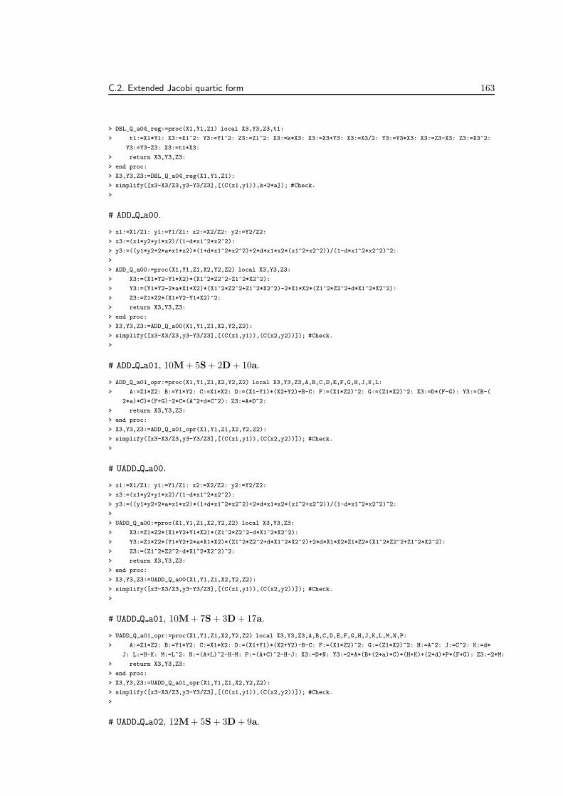
C.2. Extended Jacobi quartic form 163
> DBL_Q_a04_reg:=proc(X1,Y1,Z1) local X3,Y3,Z3,t1:
> t1:=X1*Y1: X3:=X1^2: Y3:=Y1^2: Z3:=Z1^2: X3:=k*X3: X3:=X3+Y3: X3:=X3/2: Y3:=Y3*X3: X3:=Z3-X3: Z3:=X3^2:
Y3:=Y3-Z3: X3:=t1*X3:
> return X3,Y3,Z3:
> end proc:
> X3,Y3,Z3:=DBL_Q_a04_reg(X1,Y1,Z1):
> simplify([x3-X3/Z3,y3-Y3/Z3],[(C(x1,y1)),k+2*a]); #Check.
>
# ADD Q a00.
> x1:=X1/Z1: y1:=Y1/Z1: x2:=X2/Z2: y2:=Y2/Z2:
> x3:=(x1*y2+y1*x2)/(1-d*x1^2*x2^2):
> y3:=((y1*y2+2*a*x1*x2)*(1+d*x1^2*x2^2)+2*d*x1*x2*(x1^2+x2^2))/(1-d*x1^2*x2^2)^2:
>
> ADD_Q_a00:=proc(X1,Y1,Z1,X2,Y2,Z2) local X3,Y3,Z3:
> X3:=(X1*Y2-Y1*X2)*(X1^2*Z2^2-Z1^2*X2^2):
> Y3:=(Y1*Y2-2*a*X1*X2)*(X1^2*Z2^2+Z1^2*X2^2)-2*X1*X2*(Z1^2*Z2^2+d*X1^2*X2^2):
> Z3:=Z1*Z2*(X1*Y2-Y1*X2)^2:
> return X3,Y3,Z3:
> end proc:
> X3,Y3,Z3:=ADD_Q_a00(X1,Y1,Z1,X2,Y2,Z2):
> simplify([x3-X3/Z3,y3-Y3/Z3],[(C(x1,y1)),(C(x2,y2))]); #Check.
>
# ADD Q a01, 10M + 5S + 2D + 10a.
> ADD_Q_a01_opr:=proc(X1,Y1,Z1,X2,Y2,Z2) local X3,Y3,Z3,A,B,C,D,E,F,G,H,J,K,L:
> A:=Z1*Z2: B:=Y1*Y2: C:=X1*X2: D:=(X1-Y1)*(X2+Y2)+B-C: F:=(X1*Z2)^2: G:=(Z1*X2)^2: X3:=D*(F-G): Y3:=(B-(
2*a)*C)*(F+G)-2*C*(A^2+d*C^2): Z3:=A*D^2:
> return X3,Y3,Z3:
> end proc:
> X3,Y3,Z3:=ADD_Q_a01_opr(X1,Y1,Z1,X2,Y2,Z2):
> simplify([x3-X3/Z3,y3-Y3/Z3],[(C(x1,y1)),(C(x2,y2))]); #Check.
>
# UADD Q a00.
> x1:=X1/Z1: y1:=Y1/Z1: x2:=X2/Z2: y2:=Y2/Z2:
> x3:=(x1*y2+y1*x2)/(1-d*x1^2*x2^2):
> y3:=((y1*y2+2*a*x1*x2)*(1+d*x1^2*x2^2)+2*d*x1*x2*(x1^2+x2^2))/(1-d*x1^2*x2^2)^2:
>
> UADD_Q_a00:=proc(X1,Y1,Z1,X2,Y2,Z2) local X3,Y3,Z3:
> X3:=Z1*Z2*(X1*Y2+Y1*X2)*(Z1^2*Z2^2-d*X1^2*X2^2):
> Y3:=Z1*Z2*(Y1*Y2+2*a*X1*X2)*(Z1^2*Z2^2+d*X1^2*X2^2)+2*d*X1*X2*Z1*Z2*(X1^2*Z2^2+Z1^2*X2^2):
> Z3:=(Z1^2*Z2^2-d*X1^2*X2^2)^2:
> return X3,Y3,Z3:
> end proc:
> X3,Y3,Z3:=UADD_Q_a00(X1,Y1,Z1,X2,Y2,Z2):
> simplify([x3-X3/Z3,y3-Y3/Z3],[(C(x1,y1)),(C(x2,y2))]); #Check.
>
# UADD Q a01, 10M + 7S + 3D + 17a.
> UADD_Q_a01_opr:=proc(X1,Y1,Z1,X2,Y2,Z2) local X3,Y3,Z3,A,B,C,D,E,F,G,H,J,K,L,M,N,P:
> A:=Z1*Z2: B:=Y1*Y2: C:=X1*X2: D:=(X1+Y1)*(X2+Y2)-B-C: F:=(X1*Z2)^2: G:=(Z1*X2)^2: H:=A^2: J:=C^2: K:=d*
J: L:=H-K: M:=L^2: N:=(A+L)^2-H-M: P:=(A+C)^2-H-J: X3:=D*N: Y3:=2*A*(B+(2*a)*C)*(H+K)+(2*d)*P*(F+G): Z3:=2*M:
> return X3,Y3,Z3:
> end proc:
> X3,Y3,Z3:=UADD_Q_a01_opr(X1,Y1,Z1,X2,Y2,Z2):
> simplify([x3-X3/Z3,y3-Y3/Z3],[(C(x1,y1)),(C(x2,y2))]); #Check.
>
# UADD Q a02, 12M + 5S + 3D + 9a.

164 Appendix C. Computer algebra scripts
> UADD_Q_a02_opr:=proc(X1,Y1,Z1,X2,Y2,Z2) local X3,Y3,Z3,A,B,C,D,E,F,G,H,J,K,L,M:
> A:=X1*Z2: B:=Y1*Z2: C:=Z1*X2: D:=Z1*Y2: E:=A*C: F:=B*D: G:=(A+B)*(C+D)-E-F: H:=Z1*Z2: J:=X1*X2: K:=H^2:
L:=d*J^2: M:=K-L: X3:=G*M: Z3:=M^2: Y3:=(K+L)*(F+(2*a)*E)+(2*d)*E*(A^2+C^2):
> return X3,Y3,Z3:
> end proc:
> X3,Y3,Z3:=UADD_Q_a02_opr(X1,Y1,Z1,X2,Y2,Z2):
> simplify([x3-X3/Z3,y3-Y3/Z3],[(C(x1,y1)),(C(x2,y2))]); #Check.
>
# DBL Qe a00.
> x1:=X1/Z1: y1:=Y1/Z1: T1:=X1^2/Z1:
> x3:=(2*y1/(2-y1^2+2*a*x1^2))*x1:
> y3:=(2*y1/(2-y1^2+2*a*x1^2))*((2*y1/(2-y1^2+2*a*x1^2))-y1)-1:
>
> DBL_Qe_a00:=proc(X1,Y1,Z1,T1) local X3,Y3,Z3,T3:
> X3:=2*X1*Y1*(2*Z1^2-Y1^2+2*a*X1^2):
> Y3:=2*Y1^2*(Y1^2-2*a*X1^2)-(2*Z1^2-Y1^2+2*a*X1^2)^2:
> T3:=(2*X1*Y1)^2:
> Z3:=(2*Z1^2-Y1^2+2*a*X1^2)^2:
> return X3,Y3,Z3,T3:
> end proc:
> X3,Y3,Z3,T3:=DBL_Qe_a00(X1,Y1,Z1,T1):
> simplify([x3-X3/Z3,y3-Y3/Z3,T3-X3^2/Z3],[(C(x1,y1))]); #Check.
>
# DBL Qe a01, 8S + 13a, assumes a = −1/2.
> DBL_Qe_a01_reg:=proc(X1,Y1,Z1,T1) local X3,Y3,Z3,T3,t1:
> T3:=X1+Y1: X3:=X1^2: Y3:=Y1^2: Z3:=Z1^2: T3:=T3^2: X3:=X3+Y3: T3:=T3-X3: Z3:=2*Z3: Z3:=Z3-X3: X3:=T3+Z3
: T3:=T3^2: Z3:=Z3^2: X3:=X3^2: X3:=X3-T3: X3:=X3-Z3: Z3:=2*Z3: Y3:=2*Y3: Y3:=Y3^2: Y3:=Y3+T3: Y3:=Y3-Z3: T3:=
2*T3:
> return X3,Y3,Z3,T3:
> end proc:
> X3,Y3,Z3,T3:=DBL_Qe_a01_reg(X1,Y1,Z1,T1):
> simplify([x3-X3/Z3,y3-Y3/Z3,T3-X3^2/Z3],[(C(x1,y1)),a+1/2]); #Check.
>
# DBL Qe a02, 1M + 7S + 9a, assumes a = −1/2.
> DBL_Qe_a02_reg:=proc(X1,Y1,Z1,T1) local X3,Y3,Z3,T3,t1:
> T3:=X1+Y1: X3:=X1^2: Y3:=Y1^2: Z3:=Z1^2: T3:=T3^2: X3:=X3+Y3: T3:=T3-X3: Z3:=2*Z3: Z3:=Z3-X3: X3:=T3*Z3
: Z3:=Z3^2: T3:=T3^2: Y3:=2*Y3: Y3:=Y3^2: Y3:=Y3+T3: Y3:=Y3/2: Y3:=Y3-Z3:
> return X3,Y3,Z3,T3:
> end proc:
> X3,Y3,Z3,T3:=DBL_Qe_a02_reg(X1,Y1,Z1,T1):
> simplify([x3-X3/Z3,y3-Y3/Z3,T3-X3^2/Z3],[(C(x1,y1)),a+1/2]); #Check.
>
# DBL Qe a03, 2M + 6S + 6a, assumes a = −1/2.
> DBL_Qe_a03_reg:=proc(X1,Y1,Z1,T1) local X3,Y3,Z3,T3,t1:
> T3:=X1*Y1: X3:=X1^2: Y3:=Y1^2: Z3:=Z1^2: X3:=X3+Y3: X3:=X3/2: Z3:=Z3-X3: X3:=T3*Z3: Z3:=Z3^2: T3:=T3^2:
Y3:=Y3^2: Y3:=Y3+T3: Y3:=Y3/2: Y3:=Y3-Z3:
> return X3,Y3,Z3,T3:
> end proc:
> X3,Y3,Z3,T3:=DBL_Qe_a03_reg(X1,Y1,Z1,T1):
> simplify([x3-X3/Z3,y3-Y3/Z3,T3-X3^2/Z3],[(C(x1,y1)),a+1/2]); #Check.
>
# DBL Qe a04, 3M + 5S + 4a, assumes a = −1/2.

C.2. Extended Jacobi quartic form 165
> DBL_Qe_a04_reg:=proc(X1,Y1,Z1,T1) local X3,Y3,Z3,T3,t1:
> T3:=X1*Y1: X3:=X1^2: Y3:=Y1^2: Z3:=Z1^2: X3:=X3+Y3: X3:=X3/2: Y3:=Y3*X3: X3:=Z3-X3: Z3:=X3^2: Y3:=Y3-Z3
: X3:=X3*T3: T3:=T3^2:
> return X3,Y3,Z3,T3:
> end proc:
> X3,Y3,Z3,T3:=DBL_Qe_a04_reg(X1,Y1,Z1,T1):
> simplify([x3-X3/Z3,y3-Y3/Z3,T3-X3^2/Z3],[(C(x1,y1)),a+1/2]); #Check.
>
# DBL Qe a05, 8S + 2D + 14a, assumes k = −2a.
> DBL_Qe_a05_opr:=proc(X1,Y1,Z1,T1) local X3,Y3,Z3,T3,A,B,C,D,E,F,G,H:
> A:=Z1^2: B:=Y1^2: C:=X1^2: D:=B+C: E:=(X1+Y1)^2-D: F:=2*A-B+(2*a)*C: G:=E^2: H:=F^2: X3:=(E+F)^2-G-H: T
3:=2*G: Z3:=2*H: Y3:=(2*B)^2-(2*a)*G-Z3:
> return X3,Y3,Z3,T3:
> end proc:
> X3,Y3,Z3,T3:=DBL_Qe_a05_opr(X1,Y1,Z1,T1):
> simplify([x3-X3/Z3,y3-Y3/Z3,T3-X3^2/Z3],[(C(x1,y1)),k+2*a]); #Check.
>
> DBL_Qe_a05_reg:=proc(X1,Y1,Z1,T1) local X3,Y3,Z3,T3,t1:
> T3:=X1+Y1: X3:=X1^2: Y3:=Y1^2: Z3:=Z1^2: T3:=T3^2: T3:=T3-X3: t1:=T3-Y3: X3:=k*X3: X3:=X3+Y3: Z3:=2*Z3:
Z3:=Z3-X3: T3:=t1^2: X3:=t1+Z3: X3:=X3^2: Z3:=Z3^2: X3:=X3-T3: X3:=X3-Z3: Z3:=2*Z3: t1:=k*T3: T3:=2*T3: Y3:=2
*Y3: Y3:=Y3^2: Y3:=Y3+t1: Y3:=Y3-Z3:
> return X3,Y3,Z3,T3:
> end proc:
> X3,Y3,Z3,T3:=DBL_Qe_a05_reg(X1,Y1,Z1,T1):
> simplify([x3-X3/Z3,y3-Y3/Z3,T3-X3^2/Z3],[(C(x1,y1)),k+2*a]); #Check.
>
# DBL Qe a06, 1M + 7S + 1D + 12a, assumes k = −2a.
> DBL_Qe_a06_reg:=proc(X1,Y1,Z1,T1) local X3,Y3,Z3,T3,t1:
> t1:=X1+Y1: X3:=X1^2: Y3:=Y1^2: Z3:=Z1^2: t1:=t1^2: t1:=t1-X3: t1:=t1-Y3: X3:=k*X3: X3:=X3+Y3: Z3:=2*Z3:
Y3:=X3*Y3: Z3:=Z3-X3: T3:=t1^2: X3:=t1+Z3: Z3:=Z3^2: Y3:=2*Y3: Y3:=Y3-Z3: X3:=X3^2: X3:=X3-T3: X3:=X3-Z3: X3:
=X3/2:
> return X3,Y3,Z3,T3:
> end proc:
> X3,Y3,Z3,T3:=DBL_Qe_a06_reg(X1,Y1,Z1,T1):
> simplify([x3-X3/Z3,y3-Y3/Z3,T3-X3^2/Z3],[(C(x1,y1)),k+2*a]); #Check.
>
# DBL Qe a07, 1M + 7S + 2D + 10a, assumes k = −2a.
> DBL_Qe_a07_reg:=proc(X1,Y1,Z1,T1) local X3,Y3,Z3,T3,t1:
> t1:=X1+Y1: X3:=X1^2: Y3:=Y1^2: Z3:=Z1^2: t1:=t1^2: t1:=t1-X3: t1:=t1-Y3: X3:=k*X3: X3:=X3+Y3: Z3:=2*Z3:
Z3:=Z3-X3: X3:=t1*Z3: T3:=t1^2: Z3:=Z3^2: Y3:=2*Y3: Y3:=Y3^2: t1:=k*T3: Y3:=Y3+t1: Y3:=Y3/2: Y3:=Y3-Z3:
> return X3,Y3,Z3,T3:
> end proc:
> X3,Y3,Z3,T3:=DBL_Qe_a07_reg(X1,Y1,Z1,T1):
> simplify([x3-X3/Z3,y3-Y3/Z3,T3-X3^2/Z3],[(C(x1,y1)),k+2*a]); #Check.
>
# DBL Qe a08, 2M + 6S + 1D + 8a, assumes k = −2a.
> DBL_Qe_a08_reg:=proc(X1,Y1,Z1,T1) local X3,Y3,Z3,T3,t1:
> T3:=X1+Y1: X3:=X1^2: Y3:=Y1^2: Z3:=Z1^2: T3:=T3^2: T3:=T3-X3: T3:=T3-Y3: X3:=k*X3: X3:=Y3+X3: Z3:=2*Z3:
Y3:=X3*Y3: Y3:=2*Y3: Z3:=Z3-X3: X3:=T3*Z3: Z3:=Z3^2: Y3:=Y3-Z3: T3:=T3^2:
> return X3,Y3,Z3,T3:
> end proc:
> X3,Y3,Z3,T3:=DBL_Qe_a08_reg(X1,Y1,Z1,T1):
> simplify([x3-X3/Z3,y3-Y3/Z3,T3-X3^2/Z3],[(C(x1,y1)),k+2*a]); #Check.
>
# DBL Qe a09, 2M + 6S + 2D + 6a, assumes k = −2a.

166 Appendix C. Computer algebra scripts
> DBL_Qe_a09_reg:=proc(X1,Y1,Z1,T1) local X3,Y3,Z3,T3,t1:
> t1:=X1*Y1: X3:=X1^2: Y3:=Y1^2: Z3:=Z1^2: X3:=k*X3: X3:=X3+Y3: X3:=X3/2: Z3:=Z3-X3: X3:=t1*Z3: Z3:=Z3^2:
T3:=t1^2: Y3:=Y3^2: t1:=k*T3: Y3:=Y3+t1: Y3:=Y3/2: Y3:=Y3-Z3:
> return X3,Y3,Z3,T3:
> end proc:
> X3,Y3,Z3,T3:=DBL_Qe_a09_reg(X1,Y1,Z1,T1):
> simplify([x3-X3/Z3,y3-Y3/Z3,T3-X3^2/Z3],[(C(x1,y1)),k+2*a]); #Check.
>
# DBL Qe a10, 3M + 5S + 1D + 4a, assumes k = −2a.
> DBL_Qe_a10_opr:=proc(X1,Y1,Z1,T1) local X3,Y3,Z3,T3,A,B,C,D,E,F:
> A:=Z1^2: B:=Y1^2: C:=X1^2: D:=X1*Y1: E:=(B-(2*a)*C)/2: F:=A-E: T3:=D^2: Z3:=F^2: X3:=D*F: Y3:=B*E-Z3:
> return X3,Y3,Z3,T3:
> end proc:
> X3,Y3,Z3,T3:=DBL_Qe_a10_opr(X1,Y1,Z1,T1):
> simplify([x3-X3/Z3,y3-Y3/Z3,T3-X3^2/Z3],[(C(x1,y1)),k+2*a]); #Check.
>
> DBL_Qe_a10_reg:=proc(X1,Y1,Z1,T1) local X3,Y3,Z3,T3,t1:
> T3:=X1*Y1: X3:=X1^2:Y3:=Y1^2: Z3:=Z1^2: X3:=k*X3: X3:=X3+Y3: X3:=X3/2: Y3:=Y3*X3: X3:=Z3-X3: Z3:=X3^2:
Y3:=Y3-Z3: X3:=T3*X3: T3:=T3^2:
> return X3,Y3,Z3,T3:
> end proc:
> X3,Y3,Z3,T3:=DBL_Qe_a10_reg(X1,Y1,Z1,T1):
> simplify([x3-X3/Z3,y3-Y3/Z3,T3-X3^2/Z3],[(C(x1,y1)),k+2*a]); #Check.
>
# ADD Qe a00.
> x1:=X1/Z1: y1:=Y1/Z1: T1:=X1^2/Z1: x2:=X2/Z2: y2:=Y2/Z2: T2:=X2^2/Z2:
> x3:=(x1*y2+y1*x2)/(1-d*x1^2*x2^2):
> y3:=((y1*y2+2*a*x1*x2)*(1+d*x1^2*x2^2)+2*d*x1*x2*(x1^2+x2^2))/(1-d*x1^2*x2^2)^2:
>
> ADD_Qe_a00:=proc(X1,Y1,Z1,T1,X2,Y2,Z2,T2) local X3,Y3,Z3,T3:
> X3:=(X1*Y2-Y1*X2)*(T1*Z2-Z1*T2):
> Y3:=(Y1*Y2-2*a*X1*X2)*(T1*Z2+Z1*T2)-2*X1*X2*(Z1*Z2+d*T1*T2):
> T3:=(T1*Z2-Z1*T2)^2:
> Z3:=(X1*Y2-Y1*X2)^2:
> return X3,Y3,Z3,T3:
> end proc:
> X3,Y3,Z3,T3:=ADD_Qe_a00(X1,Y1,Z1,T1,X2,Y2,Z2,T2):
> simplify([x3-X3/Z3,y3-Y3/Z3,T3-X3^2/Z3],[(C(x1,y1)),(C(x2,y2))]); #Check.
>
# ADD Qe b00.
> x1:=X1/Z1: y1:=Y1/Z1: T1:=X1^2/Z1: x2:=X2/Z2: y2:=Y2/Z2: T2:=X2^2/Z2:
> x3:=(x1*y2+y1*x2)/(1-d*x1^2*x2^2):
> y3:=((y1*y2+2*a*x1*x2)*(1+d*x1^2*x2^2)+2*d*x1*x2*(x1^2+x2^2))/(1-d*x1^2*x2^2)^2:
>
> ADD_Qe_b00:=proc(X1,Y1,Z1,T1,X2,Y2,Z2,T2) local X3,Y3,Z3,T3:
> X3:=(X1*Y2-Y1*X2)*(T1*Z2-Z1*T2):
> Y3:=(T1*Z2+Z1*T2-2*X1*X2)*(Y1*Y2-2*a*X1*X2+Z1*Z2+d*T1*T2)-(X1*Y2-Y1*X2)^2:
> T3:=(T1*Z2-Z1*T2)^2:
> Z3:=(X1*Y2-Y1*X2)^2:
> return X3,Y3,Z3,T3:
> end proc:
> X3,Y3,Z3,T3:=ADD_Qe_b00(X1,Y1,Z1,T1,X2,Y2,Z2,T2):
> simplify([x3-X3/Z3,y3-Y3/Z3,T3-X3^2/Z3],[(C(x1,y1)),(C(x2,y2))]); #Check.
>
# ADD Qe b01, 7M + 3S + 2D + 19a, assumes a = −1/2.

C.2. Extended Jacobi quartic form 167
> ADD_Qe_b01_reg:=proc(X1,Y1,Z1,T1,X2,Y2,Z2,T2) local X3,Y3,Z3,T3,t1,t2,t3:
> t1:=T1+Z1: t2:=d*T2: t2:=t2+Z2: t1:=t1*t2: t2:=Z1*T2: T3:=T1*Z2: t1:=t1-T3: t3:=d*t2: t1:=t1-t3: t3:=T3
+t2: T3:=T3-t2: Z3:=X1-Y1: t2:=X2+Y2: Z3:=Z3*t2: t2:=X1*X2: Y3:=Y1*Y2: Z3:=Z3-t2: Z3:=Z3+Y3: Y3:=Y3+t1: t1:=2*
t2: t1:=t3-t1: Y3:=Y3+t2: Y3:=t1*Y3: X3:=Z3+T3: X3:=X3^2: Z3:=Z3^2: Y3:=Y3-Z3: X3:=X3-Z3: T3:=T3^2: X3:=X3-T3:
X3:=X3/2:
> return X3,Y3,Z3,T3:
> end proc:
> X3,Y3,Z3,T3:=ADD_Qe_b01_reg(X1,Y1,Z1,T1,X2,Y2,Z2,T2):
> simplify([x3-X3/Z3,y3-Y3/Z3,T3-X3^2/Z3],[(C(x1,y1)),(C(x2,y2)),a+1/2]); #Check.
>
# ADD Qe b02, 8M + 2S + 2D + 15a, assumes a = −1/2.
> ADD_Qe_b02_reg:=proc(X1,Y1,Z1,T1,X2,Y2,Z2,T2) local X3,Y3,Z3,T3,t1,t2,t3:
> t1:=T1+Z1: t2:=d*T2: t2:=t2+Z2: t1:=t1*t2: t2:=Z1*T2: T3:=T1*Z2: t1:=t1-T3: t3:=d*t2: t1:=t1-t3: t3:=T3
+t2: T3:=T3-t2: Z3:=X1-Y1: t2:=X2+Y2: Z3:=Z3*t2: t2:=X1*X2: Y3:=Y1*Y2: Z3:=Z3-t2: Z3:=Z3+Y3: Y3:=Y3+t1: t1:=2*
t2: t1:=t3-t1: Y3:=Y3+t2: Y3:=t1*Y3: X3:=Z3*T3: Z3:=Z3^2: Y3:=Y3-Z3: T3:=T3^2:
> return X3,Y3,Z3,T3:
> end proc:
> X3,Y3,Z3,T3:=ADD_Qe_b02_reg(X1,Y1,Z1,T1,X2,Y2,Z2,T2):
> simplify([x3-X3/Z3,y3-Y3/Z3,T3-X3^2/Z3],[(C(x1,y1)),(C(x2,y2)),a+1/2]); #Check.
>
# ADD Qe b03, 7M + 3S + 3D + 19a, assumes k = −2a.
> ADD_Qe_b03_opr:=proc(X1,Y1,Z1,T1,X2,Y2,Z2,T2) local X3,Y3,Z3,T3,A,B,C,D,E,F:
> A:=T1*Z2: B:=Z1*T2: C:=X1*X2: D:=Y1*Y2: E:=(X1-Y1)*(X2+Y2)-C+D: F:=A-B: Z3:=E^2: T3:=F^2: X3:=((E+F)^2-
T3-Z3)/2: Y3:=(A+B-2*C)*(D-(2*a)*C+(Z1+T1)*(Z2+d*T2)-A-d*B)-Z3:
> return X3,Y3,Z3,T3:
> end proc:
> X3,Y3,Z3,T3:=ADD_Qe_b03_opr(X1,Y1,Z1,T1,X2,Y2,Z2,T2):
> simplify([x3-X3/Z3,y3-Y3/Z3,T3-X3^2/Z3],[(C(x1,y1)),(C(x2,y2)),k+2*a]); #Check.
>
> ADD_Qe_b03_reg:=proc(X1,Y1,Z1,T1,X2,Y2,Z2,T2) local X3,Y3,Z3,T3,t1,t2,t3:
> t1:=T1+Z1: t2:=d*T2: t2:=t2+Z2: t1:=t1*t2: t2:=Z1*T2: T3:=T1*Z2: t1:=t1-T3: t3:=d*t2: t1:=t1-t3: t3:=T3
+t2: T3:=T3-t2: Z3:=X1-Y1: t2:=X2+Y2: Z3:=Z3*t2: t2:=X1*X2: Y3:=Y1*Y2: Z3:=Z3-t2: Z3:=Z3+Y3: Y3:=Y3+t1: t1:=2*
t2: t1:=t3-t1: t2:=k*t2: Y3:=Y3+t2: Y3:=t1*Y3: X3:=Z3+T3: X3:=X3^2: Z3:=Z3^2: Y3:=Y3-Z3: X3:=X3-Z3: T3:=T3^2:
X3:=X3-T3: X3:=X3/2:
> return X3,Y3,Z3,T3:
> end proc:
> X3,Y3,Z3,T3:=ADD_Qe_b03_reg(X1,Y1,Z1,T1,X2,Y2,Z2,T2):
> simplify([x3-X3/Z3,y3-Y3/Z3,T3-X3^2/Z3],[(C(x1,y1)),(C(x2,y2)),k+2*a]); #Check.
>
# ADD Qe b04, 8M + 2S + 3D + 15a, assumes k = −2a.
> ADD_Qe_b04_opr:=proc(X1,Y1,Z1,T1,X2,Y2,Z2,T2) local X3,Y3,Z3,T3,A,B,C,D,E,F:
> A:=T1*Z2: B:=Z1*T2: C:=X1*X2: D:=Y1*Y2: E:=(X1-Y1)*(X2+Y2)-C+D: F:=A-B: Z3:=E^2: T3:=F^2: X3:=E*F: Y3:=
(A+B-2*C)*(D-(2*a)*C+(Z1+T1)*(Z2+d*T2)-A-d*B)-Z3:
> return X3,Y3,Z3,T3:
> end proc:
> X3,Y3,Z3,T3:=ADD_Qe_b04_opr(X1,Y1,Z1,T1,X2,Y2,Z2,T2):
> simplify([x3-X3/Z3,y3-Y3/Z3,T3-X3^2/Z3],[(C(x1,y1)),(C(x2,y2)),k+2*a]); #Check.
>
> ADD_Qe_b04_reg:=proc(X1,Y1,Z1,T1,X2,Y2,Z2,T2) local X3,Y3,Z3,T3,t1,t2,t3:
> t1:=T1+Z1: t2:=d*T2: t2:=t2+Z2: t1:=t1*t2: t2:=Z1*T2: T3:=T1*Z2: t1:=t1-T3: t3:=d*t2: t1:=t1-t3: t3:=T3
+t2: T3:=T3-t2: Z3:=X1-Y1: t2:=X2+Y2: Z3:=Z3*t2: t2:=X1*X2: Y3:=Y1*Y2: Z3:=Z3-t2: Z3:=Z3+Y3: Y3:=Y3+t1: t1:=2*
t2: t1:=t3-t1: t2:=k*t2: Y3:=Y3+t2: Y3:=t1*Y3: X3:=Z3*T3: Z3:=Z3^2: Y3:=Y3-Z3: T3:=T3^2:
> return X3,Y3,Z3,T3:
> end proc:
> X3,Y3,Z3,T3:=ADD_Qe_b04_reg(X1,Y1,Z1,T1,X2,Y2,Z2,T2):
> simplify([x3-X3/Z3,y3-Y3/Z3,T3-X3^2/Z3],[(C(x1,y1)),(C(x2,y2)),k+2*a]); #Check.
>

168 Appendix C. Computer algebra scripts
# UADD Qe a00.
> x1:=X1/Z1: y1:=Y1/Z1: T1:=X1^2/Z1: x2:=X2/Z2: y2:=Y2/Z2: T2:=X2^2/Z2:
> x3:=(x1*y2+y1*x2)/(1-d*x1^2*x2^2):
> y3:=((y1*y2+2*a*x1*x2)*(1+d*x1^2*x2^2)+2*d*x1*x2*(x1^2+x2^2))/(1-d*x1^2*x2^2)^2:
>
> UADD_Qe_a00:=proc(X1,Y1,Z1,T1,X2,Y2,Z2,T2) local X3,Y3,Z3,T3:
> X3:=(X1*Y2+Y1*X2)*(Z1*Z2-d*T1*T2):
> Y3:=(Y1*Y2+2*a*X1*X2)*(Z1*Z2+d*T1*T2)+2*d*X1*X2*(T1*Z2+Z1*T2):
> T3:=(X1*Y2+Y1*X2)^2:
> Z3:=(Z1*Z2-d*T1*T2)^2:
> return X3,Y3,Z3,T3:
> end proc:
> X3,Y3,Z3,T3:=UADD_Qe_a00(X1,Y1,Z1,T1,X2,Y2,Z2,T2):
> simplify([x3-X3/Z3,y3-Y3/Z3,T3-X3^2/Z3],[(C(x1,y1)),(C(x2,y2))]); #Check.
>
# UADD Qe a01, 8M + 3S + 2D + 17a, assumes a = −1/2, h = 2d.
> UADD_Qe_a01_reg:=proc(X1,Y1,Z1,T1,X2,Y2,Z2,T2) local X3,Y3,Z3,T3,t1,t2,t3:
> t1:=T1+Z1: t2:=T2+Z2: T3:=T1*T2: Z3:=Z1*Z2: t1:=t1*t2: t1:=t1-T3: t1:=t1-Z3: T3:=d*T3: t2:=Z3+T3: Z3:=Z
3-T3: T3:=X1+Y1: t3:=X2+Y2: X3:=X1*X2: Y3:=Y1*Y2: T3:=T3*t3: T3:=T3-X3: T3:=T3-Y3: t1:=h*t1: t1:=t1*X3: Y3:=Y3
-X3: Y3:=Y3*t2: Y3:=Y3+t1: X3:=Z3+T3: X3:=X3^2: T3:=T3^2: Z3:=Z3^2: X3:=X3-T3: X3:=X3-Z3: X3:=X3/2:
> return X3,Y3,Z3,T3:
> end proc:
> X3,Y3,Z3,T3:=UADD_Qe_a01_reg(X1,Y1,Z1,T1,X2,Y2,Z2,T2):
> simplify([x3-X3/Z3,y3-Y3/Z3,T3-X3^2/Z3],[(C(x1,y1)),(C(x2,y2)),a+1/2, h-2*d]); #Check.
>
# UADD Qe a02, 9M + 2S + 2D + 13a, assumes a = −1/2, h = 2d.
> UADD_Qe_a02_reg:=proc(X1,Y1,Z1,T1,X2,Y2,Z2,T2) local X3,Y3,Z3,T3,t1,t2,t3:
> t1:=T1+Z1: t2:=T2+Z2: T3:=T1*T2: Z3:=Z1*Z2: t1:=t1*t2: t1:=t1-T3: t1:=t1-Z3: T3:=d*T3: t2:=Z3+T3: Z3:=Z
3-T3: T3:=X1+Y1: t3:=X2+Y2: X3:=X1*X2: Y3:=Y1*Y2: T3:=T3*t3: T3:=T3-X3: T3:=T3-Y3: t1:=h*t1: t1:=t1*X3: Y3:=Y3
-X3: Y3:=Y3*t2: Y3:=Y3+t1: X3:=Z3*T3: T3:=T3^2: Z3:=Z3^2:
> return X3,Y3,Z3,T3:
> end proc:
> X3,Y3,Z3,T3:=UADD_Qe_a02_reg(X1,Y1,Z1,T1,X2,Y2,Z2,T2):
> simplify([x3-X3/Z3,y3-Y3/Z3,T3-X3^2/Z3],[(C(x1,y1)),(C(x2,y2)),a+1/2, h-2*d]); #Check.
>
# UADD Qe a03, 8M + 3S + 3D + 17a, assumes k = −2a, h = 2d.
> UADD_Qe_a03_opr:=proc(X1,Y1,Z1,T1,X2,Y2,Z2,T2) local X3,Y3,Z3,T3,A,B,C,D,E,F,G:
> A:=Z1*Z2: B:=T1*T2: C:=X1*X2: D:=Y1*Y2: E:=d*B: F:=(X1+Y1)*(X2+Y2)-C-D: G:=A-E: Z3:=G^2: T3:=F^2: X3:=(
(F+G)^2-T3-Z3)/2: Y3:=(D+(2*a)*C)*(A+E)+(2*d)*C*((T1+Z1)*(T2+Z2)-A-B):
> return X3,Y3,Z3,T3:
> end proc:
> X3,Y3,Z3,T3:=UADD_Qe_a03_opr(X1,Y1,Z1,T1,X2,Y2,Z2,T2):
> simplify([x3-X3/Z3,y3-Y3/Z3,T3-X3^2/Z3],[(C(x1,y1)),(C(x2,y2)),k+2*a, h-2*d]); #Check.
>
> UADD_Qe_a03_reg:=proc(X1,Y1,Z1,T1,X2,Y2,Z2,T2) local X3,Y3,Z3,T3,t1,t2,t3:
> t1:=T1+Z1: t2:=T2+Z2: T3:=T1*T2: Z3:=Z1*Z2: t1:=t1*t2: t1:=t1-T3: t1:=t1-Z3: T3:=d*T3: t2:=Z3+T3: Z3:=
Z3-T3: T3:=X1+Y1: t3:=X2+Y2: X3:=X1*X2: Y3:=Y1*Y2: T3:=T3*t3: T3:=T3-X3: T3:=T3-Y3: t1:=h*t1: t1:=t1*X3: X3:=k
*X3: Y3:=Y3-X3: Y3:=Y3*t2: Y3:=Y3+t1: X3:=Z3+T3: X3:=X3^2: T3:=T3^2: Z3:=Z3^2: X3:=X3-T3: X3:=X3-Z3: X3:=X3/2:
> return X3,Y3,Z3,T3:
> end proc:
> X3,Y3,Z3,T3:=UADD_Qe_a03_reg(X1,Y1,Z1,T1,X2,Y2,Z2,T2):
> simplify([x3-X3/Z3,y3-Y3/Z3,T3-X3^2/Z3],[(C(x1,y1)),(C(x2,y2)),k+2*a, h-2*d]); #Check.
>
# UADD Qe a04, 9M + 2S + 3D + 13a, assumes k = −2a, h = 2d.

C.2. Extended Jacobi quartic form 169
> UADD_Qe_a04_opr:=proc(X1,Y1,Z1,T1,X2,Y2,Z2,T2) local X3,Y3,Z3,T3,A,B,C,D,E,F,G:
> A:=Z1*Z2: B:=T1*T2: C:=X1*X2: D:=Y1*Y2: E:=d*B: F:=(X1+Y1)*(X2+Y2)-C-D: G:=A-E: Z3:=G^2: T3:=F^2: X3:=F
*G: Y3:=(D+(2*a)*C)*(A+E)+(2*d)*C*((T1+Z1)*(T2+Z2)-A-B):
> return X3,Y3,Z3,T3:
> end proc:
> X3,Y3,Z3,T3:=UADD_Qe_a04_opr(X1,Y1,Z1,T1,X2,Y2,Z2,T2):
> simplify([x3-X3/Z3,y3-Y3/Z3,T3-X3^2/Z3],[(C(x1,y1)),(C(x2,y2)),k+2*a, h-2*d]); #Check.
>
> UADD_Qe_a04_reg:=proc(X1,Y1,Z1,T1,X2,Y2,Z2,T2) local X3,Y3,Z3,T3,t1,t2,t3:
> t1:=T1+Z1: t2:=T2+Z2: T3:=T1*T2: Z3:=Z1*Z2: t1:=t1*t2: t1:=t1-T3: t1:=t1-Z3: T3:=d*T3: t2:=Z3+T3: Z3:=Z
3-T3: T3:=X1+Y1: t3:=X2+Y2: X3:=X1*X2: Y3:=Y1*Y2: T3:=T3*t3: T3:=T3-X3: T3:=T3-Y3: t1:=d*t1: t1:=t1*X3: t1:=2*
t1: X3:=k*X3: Y3:=Y3-X3: Y3:=Y3*t2: Y3:=Y3+t1: X3:=Z3*T3: T3:=T3^2: Z3:=Z3^2:
> return X3,Y3,Z3,T3:
> end proc:
> X3,Y3,Z3,T3:=UADD_Qe_a04_reg(X1,Y1,Z1,T1,X2,Y2,Z2,T2):
> simplify([x3-X3/Z3,y3-Y3/Z3,T3-X3^2/Z3],[(C(x1,y1)),(C(x2,y2)),k+2*a, h-2*d]); #Check.
>
# UADD Qe b00.
> x1:=X1/Z1: y1:=Y1/Z1: T1:=X1^2/Z1: x2:=X2/Z2: y2:=Y2/Z2: T2:=X2^2/Z2:
> x3:=(x1*y2+y1*x2)/(1-d*x1^2*x2^2):
> y3:=((y1*y2+2*a*x1*x2)*(1+d*x1^2*x2^2)+2*d*x1*x2*(x1^2+x2^2))/(1-d*x1^2*x2^2)^2:
>
> UADD_Qe_b00:=proc(X1,Y1,Z1,T1,X2,Y2,Z2,T2) local X3,Y3,Z3,T3:
> X3:=(X1*Y2+Y1*X2)*(Z1*Z2-d*T1*T2):
> Y3:=(Z1*Z2+d*T1*T2+2*s*X1*X2)*(Y1*Y2+2*a*X1*X2+s*T1*Z2+s*Z1*T2)-s*(X1*Y2+Y1*X2)^2:
> T3:=(X1*Y2+Y1*X2)^2:
> Z3:=(Z1*Z2-d*T1*T2)^2:
> return X3,Y3,Z3,T3:
> end proc:
> X3,Y3,Z3,T3:=UADD_Qe_b00(X1,Y1,Z1,T1,X2,Y2,Z2,T2):
> simplify([x3-X3/Z3,y3-Y3/Z3,T3-X3^2/Z3],[(C(x1,y1)),(C(x2,y2)),d-s^2]); #Check.
>
# UADD Qe b01, 7M + 3S + 1D + 18a, assumes k = −2a, d = 1.
> UADD_Qe_b01_reg:=proc(X1,Y1,Z1,T1,X2,Y2,Z2,T2) local X3,Y3,Z3,T3,t1,t2,t3:
> t1:=T1+Z1: t2:=T2+Z2: T3:=T1*T2: Z3:=Z1*Z2: t1:=t1*t2: t2:=Z3+T3: Z3:=Z3-T3: t1:=t1-t2: T3:=X1+Y1: t3:=
X2+Y2: X3:=X1*X2: Y3:=Y1*Y2: T3:=T3*t3: t3:=T3-X3: t3:=t3-Y3: T3:=t3^2: Y3:=Y3+t1: t1:=2*X3: t1:=t1+t2: t2:=k*
X3: Y3:=Y3-t2: Y3:=Y3*t1: Y3:=Y3-T3: X3:=t3+Z3: X3:=X3^2: Z3:=Z3^2: X3:=X3-Z3: X3:=X3-T3: X3:=X3/2:
> return X3,Y3,Z3,T3:
> end proc:
> X3,Y3,Z3,T3:=UADD_Qe_b01_reg(X1,Y1,Z1,T1,X2,Y2,Z2,T2):
> simplify([x3-X3/Z3,y3-Y3/Z3,T3-X3^2/Z3],[(C(x1,y1)),(C(x2,y2)),k+2*a,s-1,d-1]); #Check.
>
# UADD Qe b02, 8M + 2S + 1D + 14a, assumes k = −2a, d = 1.
> UADD_Qe_b02_reg:=proc(X1,Y1,Z1,T1,X2,Y2,Z2,T2) local X3,Y3,Z3,T3,t1,t2,t3:
> t1:=T1+Z1: t2:=T2+Z2: T3:=T1*T2: Z3:=Z1*Z2: t1:=t1*t2: t2:=Z3+T3: Z3:=Z3-T3: t1:=t1-t2: T3:=X1+Y1: t3:=
X2+Y2: X3:=X1*X2: Y3:=Y1*Y2: T3:=T3*t3: t3:=T3-X3: t3:=t3-Y3: T3:=t3^2: Y3:=Y3+t1: t1:=2*X3: t1:=t1+t2: t2:=k*
X3: Y3:=Y3-t2: Y3:=Y3*t1: Y3:=Y3-T3: X3:=t3*Z3: Z3:=Z3^2:
> return X3,Y3,Z3,T3:
> end proc:
> X3,Y3,Z3,T3:=UADD_Qe_b02_reg(X1,Y1,Z1,T1,X2,Y2,Z2,T2):
> simplify([x3-X3/Z3,y3-Y3/Z3,T3-X3^2/Z3],[(C(x1,y1)),(C(x2,y2)),k+2*a,s-1,d-1]); #Check.
>
# UADD Qe b03, 7M + 3S + 5D + 18a, assumes k = −2a, d = s2.
> UADD_Qe_b03_opr:=proc(X1,Y1,Z1,T1,X2,Y2,Z2,T2) local X3,Y3,Z3,T3,A,B,C,D,E,F,G:
> A:=Z1*Z2: B:=T1*T2: C:=X1*X2: D:=Y1*Y2: E:=d*B: F:=(X1+Y1)*(X2+Y2)-C-D: G:=A-E: Z3:=G^2: T3:=F^2: X3:=(
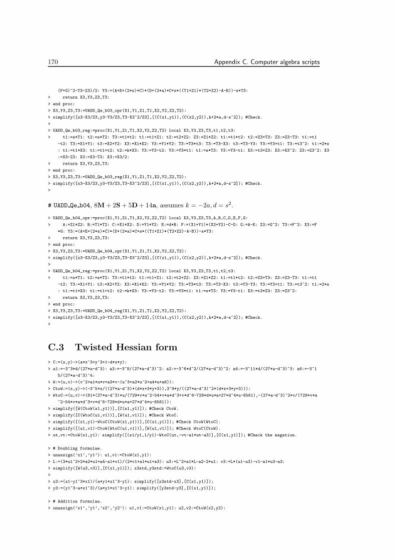
170 Appendix C. Computer algebra scripts
(F+G)^2-T3-Z3)/2: Y3:=(A+E+(2*s)*C)*(D+(2*a)*C+s*((T1+Z1)*(T2+Z2)-A-B))-s*T3:
> return X3,Y3,Z3,T3:
> end proc:
> X3,Y3,Z3,T3:=UADD_Qe_b03_opr(X1,Y1,Z1,T1,X2,Y2,Z2,T2):
> simplify([x3-X3/Z3,y3-Y3/Z3,T3-X3^2/Z3],[(C(x1,y1)),(C(x2,y2)),k+2*a,d-s^2]); #Check.
>
> UADD_Qe_b03_reg:=proc(X1,Y1,Z1,T1,X2,Y2,Z2,T2) local X3,Y3,Z3,T3,t1,t2,t3:
> t1:=s*T1: t2:=s*T2: T3:=t1*t2: t1:=t1+Z1: t2:=t2+Z2: Z3:=Z1*Z2: t1:=t1*t2: t2:=Z3+T3: Z3:=Z3-T3: t1:=t1
-t2: T3:=X1+Y1: t3:=X2+Y2: X3:=X1*X2: Y3:=Y1*Y2: T3:=T3*t3: T3:=T3-X3: t3:=T3-Y3: Y3:=Y3+t1: T3:=t3^2: t1:=2*s
: t1:=t1*X3: t1:=t1+t2: t2:=k*X3: Y3:=Y3-t2: Y3:=Y3*t1: t1:=s*T3: Y3:=Y3-t1: X3:=t3+Z3: X3:=X3^2: Z3:=Z3^2: X3
:=X3-Z3: X3:=X3-T3: X3:=X3/2:
> return X3,Y3,Z3,T3:
> end proc:
> X3,Y3,Z3,T3:=UADD_Qe_b03_reg(X1,Y1,Z1,T1,X2,Y2,Z2,T2):
> simplify([x3-X3/Z3,y3-Y3/Z3,T3-X3^2/Z3],[(C(x1,y1)),(C(x2,y2)),k+2*a,d-s^2]); #Check.
>
# UADD Qe b04, 8M + 2S + 5D + 14a, assumes k = −2a, d = s2.
> UADD_Qe_b04_opr:=proc(X1,Y1,Z1,T1,X2,Y2,Z2,T2) local X3,Y3,Z3,T3,A,B,C,D,E,F,G:
> A:=Z1*Z2: B:=T1*T2: C:=X1*X2: D:=Y1*Y2: E:=d*B: F:=(X1+Y1)*(X2+Y2)-C-D: G:=A-E: Z3:=G^2: T3:=F^2: X3:=F
*G: Y3:=(A+E+(2*s)*C)*(D+(2*a)*C+s*((T1+Z1)*(T2+Z2)-A-B))-s*T3:
> return X3,Y3,Z3,T3:
> end proc:
> X3,Y3,Z3,T3:=UADD_Qe_b04_opr(X1,Y1,Z1,T1,X2,Y2,Z2,T2):
> simplify([x3-X3/Z3,y3-Y3/Z3,T3-X3^2/Z3],[(C(x1,y1)),(C(x2,y2)),k+2*a,d-s^2]); #Check.
>
> UADD_Qe_b04_reg:=proc(X1,Y1,Z1,T1,X2,Y2,Z2,T2) local X3,Y3,Z3,T3,t1,t2,t3:
> t1:=s*T1: t2:=s*T2: T3:=t1*t2: t1:=t1+Z1: t2:=t2+Z2: Z3:=Z1*Z2: t1:=t1*t2: t2:=Z3+T3: Z3:=Z3-T3: t1:=t1
-t2: T3:=X1+Y1: t3:=X2+Y2: X3:=X1*X2: Y3:=Y1*Y2: T3:=T3*t3: T3:=T3-X3: t3:=T3-Y3: Y3:=Y3+t1: T3:=t3^2: t1:=2*s
: t1:=t1*X3: t1:=t1+t2: t2:=k*X3: Y3:=Y3-t2: Y3:=Y3*t1: t1:=s*T3: Y3:=Y3-t1: X3:=t3*Z3: Z3:=Z3^2:
> return X3,Y3,Z3,T3:
> end proc:
> X3,Y3,Z3,T3:=UADD_Qe_b04_reg(X1,Y1,Z1,T1,X2,Y2,Z2,T2):
> simplify([x3-X3/Z3,y3-Y3/Z3,T3-X3^2/Z3],[(C(x1,y1)),(C(x2,y2)),k+2*a,d-s^2]); #Check.
>
C.3 Twisted Hessian form
> C:=(x,y)->(a*x^3+y^3+1-d*x*y):
> a1:=-3^3*d/(27*a-d^3): a3:=-3^8/(27*a-d^3)^2: a2:=-3^6*d^2/(27*a-d^3)^2: a4:=-3^11*d/(27*a-d^3)^3: a6:=-3^1
5/(27*a-d^3)^4:
> W:=(u,v)->(v^2+a1*u*v+a3*v-(u^3+a2*u^2+a4*u+a6)):
> CtoW:=(x,y)->(-3^5*x/((27*a-d^3)*(d*x+3*y+3)),3^9*y/((27*a-d^3)^2*(d*x+3*y+3))):
> WtoC:=(u,v)->(81*(27*a-d^3)*u/(729*v*a^2-54*v*a*d^3+v*d^6-729*d*u*a+27*d^4*u-6561),-(27*a-d^3)^2*v/(729*v*a
^2-54*v*a*d^3+v*d^6-729*d*u*a+27*d^4*u-6561)):
> simplify([W(CtoW(x1,y1))],[C(x1,y1)]); #Check CtoW.
> simplify([C(WtoC(u1,v1))],[W(u1,v1)]); #Check WtoC.
> simplify([(x1,y1)-WtoC(CtoW(x1,y1))],[C(x1,y1)]); #Check CtoW(WtoC).
> simplify([(u1,v1)-CtoW(WtoC(u1,v1))],[W(u1,v1)]); #Check WtoC(CtoW).
> ut,vt:=CtoW(x1,y1): simplify([(x1/y1,1/y1)-WtoC(ut,-vt-a1*ut-a3)],[C(x1,y1)]); #Check the negation.
> # Doubling formulae.
> unassign(’x1’,’y1’): u1,v1:=CtoW(x1,y1):
> L:=(3*u1^2+2*a2*u1+a4-a1*v1)/(2*v1+a1*u1+a3): u3:=L^2+a1*L-a2-2*u1: v3:=L*(u1-u3)-v1-a1*u3-a3:
> simplify([W(u3,v3)],[C(x1,y1)]); x3std,y3std:=WtoC(u3,v3):
>
> x3:=(x1-y1^3*x1)/(a*y1*x1^3-y1): simplify([x3std-x3],[C(x1,y1)]);
> y3:=(y1^3-a*x1^3)/(a*y1*x1^3-y1): simplify([y3std-y3],[C(x1,y1)]);
> # Addition formulae.
> unassign(’x1’,’y1’,’x2’,’y2’): u1,v1:=CtoW(x1,y1): u2,v2:=CtoW(x2,y2):

C.3. Twisted Hessian form 171
> L:=(v2-v1)/(u2-u1): u3:=L^2+a1*L-a2-u1-u2: v3:=L*(u1-u3)-v1-a1*u3-a3:
> simplify([W(u3,v3)],[C(x1,y1),C(x2,y2)]); x3std,y3std:=WtoC(u3,v3):
>
> x3:=(y1*x2^2-x1^2*y2)/(x1*y2^2-y1^2*x2): simplify([x3std-x3],[C(x1,y1),C(x2,y2)]);
> x3:=(x1+x2-y1*y2*(x1*y2+y1*x2))/(a*x1*x2*(x1*y2+y1*x2)-y1-y2): simplify([x3std-x3],[C(x1,y1),C(x2,y2)]);
> x3:=(x1-y1^2*x2*y2)/(a*x1*y1*x2^2-y2): simplify([x3std-x3],[C(x1,y1),C(x2,y2)]);
> y3:=(x1*y1-x2*y2)/(x1*y2^2-y1^2*x2): simplify([y3std-y3],[C(x1,y1),C(x2,y2)]);
> y3:=(y1*y2*(y1+y2)-a*x1*x2*(x1+x2))/(a*x1*x2*(x1*y2+y1*x2)-y1-y2): simplify([y3std-y3],[C(x1,y1),C(x2,y2)])
;
> y3:=(y1*y2^2-a*x1^2*x2)/(a*x1*y1*x2^2-y2): simplify([y3std-y3],[C(x1,y1),C(x2,y2)]);
# DBL H a00.
> x1:=X1/Z1: y1:=Y1/Z1:
> x3:=(x1-y1^3*x1)/(a*y1*x1^3-y1):
> y3:=(y1^3-a*x1^3)/(a*y1*x1^3-y1):
>
> DBL_H_a00:=proc(X1,Y1,Z1) local X3,Y3,Z3:
> X3:=X1*(Z1^3-Y1^3):
> Y3:=Z1*(Y1^3-a*X1^3):
> Z3:=Y1*(a*X1^3-Z1^3):
> return X3,Y3,Z3:
> end proc:
> X3,Y3,Z3:=DBL_H_a00(X1,Y1,Z1):
> simplify([x3-X3/Z3,y3-Y3/Z3],[(C(x1,y1))]); #Check.
>
# DBL H a01, 6M + 3S + 1D + 3a.
> DBL_H_a01_opr:=proc(X1,Y1,Z1) local X3,Y3,Z3,A,B,C,D,E,F,G:
> A:=X1^2: B:=Y1^2: C:=Z1^2: D:=X1*A: E:=Y1*B: F:=Z1*C: G:=a*D: X3:=X1*(E-F): Y3:=Z1*(G-E): Z3:=Y1*(F-G):
> return X3,Y3,Z3:
> end proc:
> X3,Y3,Z3:=DBL_H_a01_opr(X1,Y1,Z1):
> simplify([x3-X3/Z3,y3-Y3/Z3],[(C(x1,y1))]); #Check.
>
> DBL_H_a01_reg:=proc(X1,Y1,Z1) local X3,Y3,Z3,t1,t2,t3,t4,t:
> t1:=Z1^2: t1:=Z1*t1: t2:=Y1^2: t2:=Y1*t2: t3:=X1^2: t3:=X1*t3: t3:=a*t3: t4:=t2-t1: X3:=X1*t4: t2:=t3-t
2: Z3:=Z1*t2: t1:=t1-t3: Y3:=Y1*t1: t:=Y3: Y3:=Z3: Z3:=t:
> return X3,Y3,Z3:
> end proc:
> X3,Y3,Z3:=DBL_H_a01_reg(X1,Y1,Z1):
> simplify([x3-X3/Z3,y3-Y3/Z3],[(C(x1,y1))]); #Check.
>
# DBL H a02, 3M + 6S + 18a, assumes a = 1.
> DBL_H_a02_opr:=proc(X1,Y1,Z1) local X3,Y3,Z3,A,B,C,D,E,F,G,H,J:
> A:=X1^2: B:=Y1^2: C:=Z1^2: D:=A+B: E:=A+C: F:=B+C: G:=((X1+Y1)^2-D)/2: H:=((X1+Z1)^2-E)/2: J:=((Y1+Z1)^
2-F)/2: X3:=(H-G)*(F+J): Y3:=(J-H)*(D+G): Z3:=(G-J)*(E+H):
> return X3,Y3,Z3:
> end proc:
> X3,Y3,Z3:=DBL_H_a02_opr(X1,Y1,Z1):
> simplify([x3-X3/Z3,y3-Y3/Z3],[(C(x1,y1)),a-1]); #Check.
>
> DBL_H_a02_reg:=proc(X1,Y1,Z1) local X3,Y3,Z3,t1,t2,t3,t4,t5,t6:
> t1:=X1^2: t2:=Y1^2: t3:=Z1^2: t4:=t1+t2: t5:=t1+t3: t6:=t2+t3: t1:=X1+Y1: t1:=t1^2: t1:=t1-t4: t1:=t1/2
: t2:=X1+Z1: t2:=t2^2: t2:=t2-t5: t2:=t2/2: t3:=Y1+Z1: t3:=t3^2: t3:=t3-t6: t3:=t3/2: X3:=t2-t1: Y3:=t3-t2: Z3
:=t1-t3: t3:=t6+t3: X3:=X3*t3: t1:=t4+t1: Y3:=Y3*t1: t2:=t5+t2: Z3:=Z3*t2:
> return X3,Y3,Z3:
> end proc:
> X3,Y3,Z3:=DBL_H_a02_reg(X1,Y1,Z1):
> simplify([x3-X3/Z3,y3-Y3/Z3],[(C(x1,y1)),a-1]); #Check.
>

172 Appendix C. Computer algebra scripts
# DBL H a03, 7M + 1S + 8a, assumes a = 1.
> DBL_H_a03_opr:=proc(X1,Y1,Z1) local X3,Y3,Z3,A,B,C:
> A:=Y1^2: B:=(Z1-Y1)*(A+(Y1+Z1)*Z1): C:=(Y1-X1)*(X1*(X1+Y1)+A): X3:=X1*B: Y3:=Z1*C: Z3:=Y1*(-B-C):
> return X3,Y3,Z3:
> end proc:
> X3,Y3,Z3:=DBL_H_a03_opr(X1,Y1,Z1):
> simplify([x3-X3/Z3,y3-Y3/Z3],[(C(x1,y1)),a-1]); #Check.
>
> DBL_H_a03_reg:=proc(X1,Y1,Z1) local X3,Y3,Z3,t1,t2,t3,t:
> t1:=Y1^2: t2:=Y1+Z1: t2:=t2*Z1: t2:=t1+t2: t3:=Z1-Y1: t2:=t3*t2: t3:=X1+Y1: t3:=X1*t3: t3:=t3+t1: t1:=Y
1-X1: t1:=t1*t3: X3:=X1*t2: Z3:=Z1*t1: t1:=-t1: t1:=t1-t2: Y3:=Y1*t1: t:=Y3: Y3:=Z3: Z3:=t:
> return X3,Y3,Z3:
> end proc:
> X3,Y3,Z3:=DBL_H_a03_reg(X1,Y1,Z1):
> simplify([x3-X3/Z3,y3-Y3/Z3],[(C(x1,y1)),a-1]); #Check.
>
# ADD H a00.
> x1:=X1/Z1: y1:=Y1/Z1: x2:=X2/Z2: y2:=Y2/Z2:
> x3:=(x1-y1^2*x2*y2)/(a*x1*y1*x2^2-y2):
> y3:=(y1*y2^2-a*x1^2*x2)/(a*x1*y1*x2^2-y2):
>
> ADD_H_a00:=proc(X1,Y1,Z1,X2,Y2,Z2) local X3,Y3,Z3:
> X3:=X1^2*Y2*Z2-Y1*Z1*X2^2:
> Y3:=Z1^2*X2*Y2-X1*Y1*Z2^2:
> Z3:=Y1^2*X2*Z2-X1*Z1*Y2^2:
> return X3,Y3,Z3:
> end proc:
> X3,Y3,Z3:=ADD_H_a00(X1,Y1,Z1,X2,Y2,Z2):
> simplify([x3-X3/Z3,y3-Y3/Z3],[(C(x1,y1)),(C(x2,y2))]); #Check.
>
# ADD H a01, 12M + 3a.
> ADD_H_a01_opr:=proc(X1,Y1,Z1,X2,Y2,Z2) local X3,Y3,Z3,A,B,C,D,E,F:
> A:=X1*Z2: B:=Y1*Z2: C:=Z1*X2: D:=Z1*Y2: E:=X1*Y2: F:=Y1*X2: X3:=E*A-F*C: Y3:=C*D-A*B: Z3:=F*B-E*D:
> return X3,Y3,Z3:
> end proc:
> X3,Y3,Z3:=ADD_H_a01_opr(X1,Y1,Z1,X2,Y2,Z2):
> simplify([x3-X3/Z3,y3-Y3/Z3],[(C(x1,y1)),(C(x2,y2))]); #Check.
>
> ADD_H_a01_reg:=proc(X1,Y1,Z1,X2,Y2,Z2) local X3,Y3,Z3,t1,t2,t3,t4,t5,t6:
> t1:=X1*Z2: t2:=Y1*Z2: t3:=Z1*X2: t4:=Z1*Y2: t5:=X1*Y2: t6:=Y1*X2: X3:=t5*t1: Y3:=t3*t4: Z3:=t6*t2: t3:=
t6*t3: X3:=X3-t3: t1:=t1*t2: Y3:=Y3-t1: t4:=t5*t4: Z3:=Z3-t4:
> return X3,Y3,Z3:
> end proc:
> X3,Y3,Z3:=ADD_H_a01_reg(X1,Y1,Z1,X2,Y2,Z2):
> simplify([x3-X3/Z3,y3-Y3/Z3],[(C(x1,y1)),(C(x2,y2))]); #Check.
>
# ADD H a02, 11M + 17a.
> ADD_H_a02_opr:=proc(X1,Y1,Z1,X2,Y2,Z2) local X3,Y3,Z3,A,B,C,D,E,F,G,H,J,K:
> A:=X1*Z2: B:=Y1*Z2: C:=Z1*X2: D:=Z1*Y2: E:=X1*Y2: F:=Y1*X2: G:=(C+E)*(A-F): H:=(C-E)*(A+F): J:=(C+B)*(A
-D): K:=(C-B)*(A+D): X3:=G-H: Y3:=K-J: Z3:=J+K-G-H-2*(E-B)*(F+D):
> return X3,Y3,Z3:
> end proc:
> X3,Y3,Z3:=ADD_H_a02_opr(X1,Y1,Z1,X2,Y2,Z2):
> simplify([x3-X3/Z3,y3-Y3/Z3],[(C(x1,y1)),(C(x2,y2))]); #Check.
>
> ADD_H_a02_reg:=proc(X1,Y1,Z1,X2,Y2,Z2) local X3,Y3,Z3,t1,t2,t3,t4,t5,t6:
> t1:=X1*Z2: t2:=Y1*Z2: t3:=Z1*X2: t4:=Z1*Y2: t5:=X1*Y2: t6:=Y1*X2: X3:=t3+t5: Y3:=t1-t6: X3:=X3*Y3: Y3:=
C.3. Twisted Hessian form 173
t5-t2: Z3:=t6+t4: Z3:=Y3*Z3: Z3:=2*Z3: Z3:=X3+Z3: t5:=t3-t5: t6:=t1+t6: t5:=t5*t6: X3:=X3-t5: t6:=t3+t2: Y3:=t
1-t4: Y3:=t6*Y3: t2:=t3-t2: t1:=t1+t4: t1:=t2*t1: t2:=t1-t5: t2:=Y3+t2: Z3:=t2-Z3: Y3:=t1-Y3:
> return X3,Y3,Z3:
> end proc:
> X3,Y3,Z3:=ADD_H_a02_reg(X1,Y1,Z1,X2,Y2,Z2):
> simplify([x3-X3/Z3,y3-Y3/Z3],[(C(x1,y1)),(C(x2,y2))]); #Check.
>
# UADD H a00.
> x1:=X1/Z1: y1:=Y1/Z1: x2:=X2/Z2: y2:=Y2/Z2:
> x3:=(x1-y1^2*x2*y2)/(a*x1*y1*x2^2-y2):
> y3:=(y1*y2^2-a*x1^2*x2)/(a*x1*y1*x2^2-y2):
>
> UADD_H_a00:=proc(X1,Y1,Z1,X2,Y2,Z2) local X3,Y3,Z3:
> X3:=X1*Z1*Z2^2-Y1^2*X2*Y2:
> Y3:=Y1*Z1*Y2^2-a*X1^2*X2*Z2:
> Z3:=a*X1*Y1*X2^2-Z1^2*Z2*Y2:
> return X3,Y3,Z3:
> end proc:
> X3,Y3,Z3:=UADD_H_a00(X1,Y1,Z1,X2,Y2,Z2):
> simplify([x3-X3/Z3,y3-Y3/Z3],[(C(x1,y1)),(C(x2,y2))]); #Check.
>
# UADD H a01, 12M + 3a.
> UADD_H_a01_opr:=proc(X1,Y1,Z1,X2,Y2,Z2) local X3,Y3,Z3,A,B,C,D,E,F:
> A:=X1*Z2: B:=Z1*Z2: C:=Y1*X2: D:=Y1*Y2: E:=Z1*Y2: F:=a*X1*X2: X3:=A*B-C*D: Y3:=D*E-F*A: Z3:=F*C-B*E:
> return X3,Y3,Z3:
> end proc:
> X3,Y3,Z3:=UADD_H_a01_opr(X1,Y1,Z1,X2,Y2,Z2):
> simplify([x3-X3/Z3,y3-Y3/Z3],[(C(x1,y1)),(C(x2,y2))]); #Check.
>
> UADD_H_a01_reg:=proc(X1,Y1,Z1,X2,Y2,Z2) local X3,Y3,Z3,t1,t2,t3,t4,t5,t6:
> t1:=X1*Z2: t2:=Z1*Z2: t3:=Y1*X2: t4:=Y1*Y2: t5:=Z1*Y2: t6:=X1*X2: t6:=a*t6: X3:=t1*t2: Y3:=t4*t5: Z3:=t
6*t3: t3:=t3*t4: t1:=t6*t1: t2:=t2*t5: X3:=X3-t3: Y3:=Y3-t1: Z3:=Z3-t2:
> return X3,Y3,Z3:
> end proc:
> X3,Y3,Z3:=UADD_H_a01_reg(X1,Y1,Z1,X2,Y2,Z2):
> simplify([x3-X3/Z3,y3-Y3/Z3],[(C(x1,y1)),(C(x2,y2))]); #Check.
>
# UADD H a02, 11M + 17a.
> UADD_H_a02_opr:=proc(X1,Y1,Z1,X2,Y2,Z2) local X3,Y3,Z3,A,B,C,D,E,F,G,H,J,K:
> A:=X1*Z2: B:=Z1*Z2: C:=Y1*X2: D:=Y1*Y2: E:=Z1*Y2: F:=a*X1*X2: G:=(D+B)*(A-C): H:=(D-B)*(A+C): J:=(D+F)*
(A-E): K:=(D-F)*(A+E): X3:=G-H: Y3:=K-J: Z3:=J+K-G-H-2*(B-F)*(C+E):
> return X3,Y3,Z3:
> end proc:
> X3,Y3,Z3:=UADD_H_a02_opr(X1,Y1,Z1,X2,Y2,Z2):
> simplify([x3-X3/Z3,y3-Y3/Z3],[(C(x1,y1)),(C(x2,y2))]); #Check.
>
> UADD_H_a02_reg:=proc(X1,Y1,Z1,X2,Y2,Z2) local X3,Y3,Z3,t1,t2,t3,t4,t5,t6:
> t1:=X1*Z2: t2:=Z1*Z2: t3:=Y1*X2: t4:=Y1*Y2: Z3:=Z1*Y2: X3:=X1*X2: X3:=a*X3: Y3:=t2-X3: Y3:=2*Y3: t5:=t3
+Z3: Y3:=Y3*t5: t5:=t4+t2: t2:=t4-t2: t6:=t1-t3: t3:=t1+t3: t2:=t2*t3: t3:=t5*t6: t5:=t4+X3: t4:=t4-X3: X3:=t3
-t2: Y3:=Y3+t2: t2:=t1-Z3: t2:=t5*t2: Y3:=Y3-t2: t1:=t1+Z3: t1:=t4*t1: Y3:=t1-Y3: Z3:=Y3-t3: Y3:=t1-t2:
> return X3,Y3,Z3:
> end proc:
> X3,Y3,Z3:=UADD_H_a02_reg(X1,Y1,Z1,X2,Y2,Z2):
> simplify([x3-X3/Z3,y3-Y3/Z3],[(C(x1,y1)),(C(x2,y2))]); #Check.
>
# DBL He a00.
174 Appendix C. Computer algebra scripts
> x1:=X1/Z1: y1:=Y1/Z1: R1:=X1*Y1/Z1: S1:=X1^2/Z1: T1:=Y1^2/Z1:
> x3:=(x1-y1^3*x1)/(a*y1*x1^3-y1):
> y3:=(y1^3-a*x1^3)/(a*y1*x1^3-y1):
>
> DBL_He_a00:=proc(X1,Y1,Z1,R1,S1,T1) local X3,Y3,Z3,R3,S3,T3:
> X3:=(X1*Z1-R1*T1)*(a*R1*S1-Y1*Z1):
> Y3:=(Y1*T1-a*X1*S1)*(a*R1*S1-Y1*Z1):
> R3:=(X1*Z1-R1*T1)*(Y1*T1-a*X1*S1):
> S3:=(X1*Z1-R1*T1)^2:
> T3:=(Y1*T1-a*X1*S1)^2:
> Z3:=(a*R1*S1-Y1*Z1)^2:
> return X3,Y3,Z3,R3,S3,T3:
> end proc:
> X3,Y3,Z3,R3,S3,T3:=DBL_He_a00(X1,Y1,Z1,R1,S1,T1):
> simplify([x3-X3/Z3,y3-Y3/Z3,R3-X3*Y3/Z3,S3-X3^2/Z3,T3-Y3^2/Z3],[(C(x1,y1))]); #Check.
>
# DBL He a01, 9M + 3S + 1D + 3a.
> DBL_He_a01_opr:=proc(X1,Y1,Z1,R1,S1,T1) local X3,Y3,Z3,R3,S3,T3,A,B,C,D:
> A:=a*S1: B:=X1*Z1-T1*R1: C:=Y1*T1-A*X1: D:=R1*A-Z1*Y1: X3:=B*D: Y3:=C*D: R3:=B*C: S3:=B^2: T3:=C^2: Z3:
=D^2:
> return X3,Y3,Z3,R3,S3,T3:
> end proc:
> X3,Y3,Z3,R3,S3,T3:=DBL_He_a01_opr(X1,Y1,Z1,R1,S1,T1):
> simplify([x3-X3/Z3,y3-Y3/Z3,R3-X3*Y3/Z3,S3-X3^2/Z3,T3-Y3^2/Z3],[(C(x1,y1))]); #Check.
>
> DBL_He_a01_reg:=proc(X1,Y1,Z1,R1,S1,T1) local X3,Y3,Z3,R3,S3,T3,t1:
> t1:=X1*Z1: S3:=a*S1: X3:=S3*X1: S3:=R1*S3: R3:=T1*R1: T3:=Y1*T1: Y3:=Z1*Y1: R3:=t1-R3: t1:=T3-X3: Y3:=S
3-Y3: S3:=R3^2: T3:=t1^2: Z3:=Y3^2: X3:=R3*Y3: Y3:=t1*Y3: R3:=R3*t1:
> return X3,Y3,Z3,R3,S3,T3:
> end proc:
> X3,Y3,Z3,R3,S3,T3:=DBL_He_a01_reg(X1,Y1,Z1,R1,S1,T1):
> simplify([x3-X3/Z3,y3-Y3/Z3,R3-X3*Y3/Z3,S3-X3^2/Z3,T3-Y3^2/Z3],[(C(x1,y1))]); #Check.
>
# DBL He a02, 5M + 6S + 1D + 29a.
> DBL_He_a02_opr:=proc(X1,Y1,Z1,R1,S1,T1) local X3,Y3,Z3,R3,S3,T3,A,B,C,D,E,F,G,H:
> A:=a*S1: B:=(T1+Z1)*(X1-R1): C:=(T1-Z1)*(X1+R1): D:=(T1+A)*(X1-Y1): E:=(T1-A)*(X1+Y1): F:=B-C: G:=E-D:
H:=D+E-B-C-2*(Z1-A)*(R1+Y1): S3:=F^2: T3:=G^2: Z3:=H^2: X3:=((F+H)^2-S3-Z3)/2: Y3:=((G+H)^2-T3-Z3)/2: R3:=((F+
G)^2-S3-T3)/2:
> return X3,Y3,Z3,R3,S3,T3:
> end proc:
> X3,Y3,Z3,R3,S3,T3:=DBL_He_a02_opr(X1,Y1,Z1,R1,S1,T1):
> simplify([x3-X3/Z3,y3-Y3/Z3,R3-X3*Y3/Z3,S3-X3^2/Z3,T3-Y3^2/Z3],[(C(x1,y1))]); #Check.
>
> DBL_He_a02_reg:=proc(X1,Y1,Z1,R1,S1,T1) local X3,Y3,Z3,R3,S3,T3,t1,t2,t3:
> S3:=a*S1: t1:=Z1-S3: t1:=2*t1: t2:=R1+Y1: t1:=t1*t2: t2:=X1-Y1: Y3:=X1+Y1: t3:=T1+S3: t2:=t3*t2: t1:=t2
-t1: t3:=T1-S3: t3:=t3*Y3: t1:=t1+t3: t2:=t3-t2: t3:=T1+Z1: Y3:=X1-R1: t3:=t3*Y3: t1:=t1-t3: Z3:=T1-Z1: X3:=X1
+R1: X3:=Z3*X3: t3:=t3-X3: t1:=t1-X3: S3:=t3^2: T3:=t2^2: Z3:=t1^2: X3:=t3+t1: X3:=X3^2: X3:=X3-S3: X3:=X3-Z3:
X3:=X3/2: Y3:=t2+t1: Y3:=Y3^2: Y3:=Y3-T3: Y3:=Y3-Z3: Y3:=Y3/2: R3:=t3+t2: R3:=R3^2: R3:=R3-S3: R3:=R3-T3: R3:
=R3/2:
> return X3,Y3,Z3,R3,S3,T3:
> end proc:
> X3,Y3,Z3,R3,S3,T3:=DBL_He_a02_reg(X1,Y1,Z1,R1,S1,T1):
> simplify([x3-X3/Z3,y3-Y3/Z3,R3-X3*Y3/Z3,S3-X3^2/Z3,T3-Y3^2/Z3],[(C(x1,y1))]); #Check.
>
# ADD He a00.
> x1:=X1/Z1: y1:=Y1/Z1: R1:=X1*Y1/Z1: S1:=X1^2/Z1: T1:=Y1^2/Z1: x2:=X2/Z2: y2:=Y2/Z2: R2:=X2*Y2/Z2: S2:=X2^2/
Z2: T2:=Y2^2/Z2:

C.3. Twisted Hessian form 175
> x3:=(x1-y1^2*x2*y2)/(a*x1*y1*x2^2-y2):
> y3:=(y1*y2^2-a*x1^2*x2)/(a*x1*y1*x2^2-y2):
>
> ADD_He_a00:=proc(X1,Y1,Z1,R1,S1,T1,X2,Y2,Z2,R2,S2,T2) local X3,Y3,Z3,R3,S3,T3:
> X3:=(S1*Y2-Y1*S2)*(T1*X2-X1*T2):
> Y3:=(Z1*R2-R1*Z2)*(T1*X2-X1*T2):
> R3:=(S1*Y2-Y1*S2)*(Z1*R2-R1*Z2):
> S3:=(S1*Y2-Y1*S2)^2:
> T3:=(Z1*R2-R1*Z2)^2:
> Z3:=(T1*X2-X1*T2)^2:
> return X3,Y3,Z3,R3,S3,T3:
> end proc:
> X3,Y3,Z3,R3,S3,T3:=ADD_He_a00(X1,Y1,Z1,R1,S1,T1,X2,Y2,Z2,R2,S2,T2):
> simplify([x3-X3/Z3,y3-Y3/Z3,R3-X3*Y3/Z3,S3-X3^2/Z3,T3-Y3^2/Z3],[(C(x1,y1)),(C(x2,y2))]); #Check.
>
# ADD He a01, 9M + 3S + 3a.
> ADD_He_a01_opr:=proc(X1,Y1,Z1,R1,S1,T1,X2,Y2,Z2,R2,S2,T2) local X3,Y3,Z3,R3,S3,T3,A,B,C:
> A:=S1*Y2-Y1*S2: B:=Z1*R2-R1*Z2: C:=T1*X2-X1*T2: X3:=A*C: Y3:=B*C: R3:=A*B: S3:=A^2: T3:=B^2: Z3:=C^2:
> return X3,Y3,Z3,R3,S3,T3:
> end proc:
> X3,Y3,Z3,R3,S3,T3:=ADD_He_a01_opr(X1,Y1,Z1,R1,S1,T1,X2,Y2,Z2,R2,S2,T2):
> simplify([x3-X3/Z3,y3-Y3/Z3,R3-X3*Y3/Z3,S3-X3^2/Z3,T3-Y3^2/Z3],[(C(x1,y1)),(C(x2,y2))]); #Check.
>
> ADD_He_a01_reg:=proc(X1,Y1,Z1,R1,S1,T1,X2,Y2,Z2,R2,S2,T2) local X3,Y3,Z3,R3,S3,T3,t1:
> t1:=R1*Z2: Z3:=Z1*R2: Z3:=Z3-t1: t1:=Y1*S2: S3:=S1*Y2: S3:=S3-t1: t1:=T1*X2: X3:=X1*T2: t1:=t1-X3: X3:=
S3*t1: Y3:=Z3*t1: R3:=S3*Z3: S3:=S3^2: T3:=Z3^2: Z3:=t1^2:
> return X3,Y3,Z3,R3,S3,T3:
> end proc:
> X3,Y3,Z3,R3,S3,T3:=ADD_He_a01_reg(X1,Y1,Z1,R1,S1,T1,X2,Y2,Z2,R2,S2,T2):
> simplify([x3-X3/Z3,y3-Y3/Z3,R3-X3*Y3/Z3,S3-X3^2/Z3,T3-Y3^2/Z3],[(C(x1,y1)),(C(x2,y2))]); #Check.
>
# ADD He a02, 6M + 6S + 15a.
> ADD_He_a02_opr:=proc(X1,Y1,Z1,R1,S1,T1,X2,Y2,Z2,R2,S2,T2) local X3,Y3,Z3,R3,S3,T3,A,B,C:
> A:=S1*Y2-Y1*S2: B:=Z1*R2-R1*Z2: C:=T1*X2-X1*T2: S3:=A^2: T3:=B^2: Z3:=C^2: X3:=((A+C)^2-S3-Z3)/2: Y3:=(
(B+C)^2-T3-Z3)/2: R3:=((A+B)^2-S3-T3)/2:
> return X3,Y3,Z3,R3,S3,T3:
> end proc:
> X3,Y3,Z3,R3,S3,T3:=ADD_He_a02_opr(X1,Y1,Z1,R1,S1,T1,X2,Y2,Z2,R2,S2,T2):
> simplify([x3-X3/Z3,y3-Y3/Z3,R3-X3*Y3/Z3,S3-X3^2/Z3,T3-Y3^2/Z3],[(C(x1,y1)),(C(x2,y2))]); #Check.
>
> ADD_He_a02_reg:=proc(X1,Y1,Z1,R1,S1,T1,X2,Y2,Z2,R2,S2,T2) local X3,Y3,Z3,R3,S3,T3,t1:
> t1:=R1*Z2: R3:=Z1*R2: R3:=R3-t1: t1:=X1*T2: X3:=T1*X2: X3:=X3-t1: t1:=Y1*S2: Y3:=S1*Y2: t1:=Y3-t1: S3:=
t1^2: T3:=R3^2: Z3:=X3^2: Y3:=R3+X3: Y3:=Y3^2: Y3:=Y3-T3: Y3:=Y3-Z3: Y3:=Y3/2: X3:=t1+X3: X3:=X3^2: X3:=X3-S3:
X3:=X3-Z3: X3:=X3/2: R3:=t1+R3: R3:=R3^2: R3:=R3-S3: R3:=R3-T3: R3:=R3/2:
> return X3,Y3,Z3,R3,S3,T3:
> end proc:
> X3,Y3,Z3,R3,S3,T3:=ADD_He_a02_reg(X1,Y1,Z1,R1,S1,T1,X2,Y2,Z2,R2,S2,T2):
> simplify([x3-X3/Z3,y3-Y3/Z3,R3-X3*Y3/Z3,S3-X3^2/Z3,T3-Y3^2/Z3],[(C(x1,y1)),(C(x2,y2))]); #Check.
>
# UADD He a00.
> x1:=X1/Z1: y1:=Y1/Z1: R1:=X1*Y1/Z1: S1:=X1^2/Z1: T1:=Y1^2/Z1: x2:=X2/Z2: y2:=Y2/Z2: R2:=X2*Y2/Z2: S2:=X2^2/
Z2: T2:=Y2^2/Z2:
> x3:=(x1-y1^2*x2*y2)/(a*x1*y1*x2^2-y2):
> y3:=(y1*y2^2-a*x1^2*x2)/(a*x1*y1*x2^2-y2):
>
> UADD_He_a00:=proc(X1,Y1,Z1,R1,S1,T1,X2,Y2,Z2,R2,S2,T2) local X3,Y3,Z3,R3,S3,T3:
> X3:=(X1*Z2-T1*R2)*(a*R1*S2-Z1*Y2):

176 Appendix C. Computer algebra scripts
> Y3:=(Y1*T2-a*S1*X2)*(a*R1*S2-Z1*Y2):
> R3:=(X1*Z2-T1*R2)*(Y1*T2-a*S1*X2):
> S3:=(X1*Z2-T1*R2)^2:
> T3:=(Y1*T2-a*S1*X2)^2:
> Z3:=(a*R1*S2-Z1*Y2)^2:
> return X3,Y3,Z3,R3,S3,T3:
> end proc:
> X3,Y3,Z3,R3,S3,T3:=UADD_He_a00(X1,Y1,Z1,R1,S1,T1,X2,Y2,Z2,R2,S2,T2):
> simplify([x3-X3/Z3,y3-Y3/Z3,R3-X3*Y3/Z3,S3-X3^2/Z3,T3-Y3^2/Z3],[(C(x1,y1)),(C(x2,y2))]); #Check.
>
# UADD He a01, 9M + 3S + 2D + 3a.
> UADD_He_a01_opr:=proc(X1,Y1,Z1,R1,S1,T1,X2,Y2,Z2,R2,S2,T2) local X3,Y3,Z3,R3,S3,T3,A,B,C:
> A:=X1*Z2-T1*R2: B:=Y1*T2-a*S1*X2: C:=a*R1*S2-Z1*Y2: X3:=A*C: Y3:=B*C: R3:=A*B: S3:=A^2: T3:=B^2: Z3:=C^
2:
> return X3,Y3,Z3,R3,S3,T3:
> end proc:
> X3,Y3,Z3,R3,S3,T3:=UADD_He_a01_opr(X1,Y1,Z1,R1,S1,T1,X2,Y2,Z2,R2,S2,T2):
> simplify([x3-X3/Z3,y3-Y3/Z3,R3-X3*Y3/Z3,S3-X3^2/Z3,T3-Y3^2/Z3],[(C(x1,y1)),(C(x2,y2))]); #Check.
>
> UADD_He_a01_reg:=proc(X1,Y1,Z1,R1,S1,T1,X2,Y2,Z2,R2,S2,T2) local X3,Y3,Z3,R3,S3,T3,t1:
> t1:=X1*Z2: Z3:=Z1*Y2: Y3:=Y1*T2: T3:=T1*R2: R3:=R1*S2: S3:=S1*X2: S3:=a*S3: R3:=a*R3: t1:=t1-T3: Y3:=Y3
-S3: Z3:=R3-Z3: X3:=t1*Z3: R3:=t1*Y3: S3:=t1^2: T3:=Y3^2: Y3:=Y3*Z3: Z3:=Z3^2:
> return X3,Y3,Z3,R3,S3,T3:
> end proc:
> X3,Y3,Z3,R3,S3,T3:=UADD_He_a01_reg(X1,Y1,Z1,R1,S1,T1,X2,Y2,Z2,R2,S2,T2):
> simplify([x3-X3/Z3,y3-Y3/Z3,R3-X3*Y3/Z3,S3-X3^2/Z3,T3-Y3^2/Z3],[(C(x1,y1)),(C(x2,y2))]); #Check.
>
# UADD He a02, 6M + 6S + 2D + 15a.
> UADD_He_a02_opr:=proc(X1,Y1,Z1,R1,S1,T1,X2,Y2,Z2,R2,S2,T2) local X3,Y3,Z3,R3,S3,T3,A,B,C:
> A:=X1*Z2-T1*R2: B:=Y1*T2-a*S1*X2: C:=a*R1*S2-Z1*Y2: S3:=A^2: T3:=B^2: Z3:=C^2: X3:=((A+C)^2-S3-Z3)/2: Y
3:=((B+C)^2-T3-Z3)/2: R3:=((A+B)^2-S3-T3)/2:
> return X3,Y3,Z3,R3,S3,T3:
> end proc:
> X3,Y3,Z3,R3,S3,T3:=UADD_He_a02_opr(X1,Y1,Z1,R1,S1,T1,X2,Y2,Z2,R2,S2,T2):
> simplify([x3-X3/Z3,y3-Y3/Z3,R3-X3*Y3/Z3,S3-X3^2/Z3,T3-Y3^2/Z3],[(C(x1,y1)),(C(x2,y2))]); #Check.
>
> UADD_He_a02_reg:=proc(X1,Y1,Z1,R1,S1,T1,X2,Y2,Z2,R2,S2,T2) local X3,Y3,Z3,R3,S3,T3,t1:
> t1:=X1*Z2: Z3:=Z1*Y2: Y3:=Y1*T2: T3:=T1*R2: R3:=R1*S2: S3:=S1*X2: S3:=a*S3: R3:=a*R3: t1:=t1-T3: Y3:=Y3
-S3: X3:=R3-Z3: S3:=t1^2: T3:=Y3^2: Z3:=X3^2: R3:=t1+Y3: R3:=R3^2: R3:=R3-S3: R3:=R3-T3: R3:=R3/2: Y3:=Y3+X3:
Y3:=Y3^2: Y3:=Y3-T3: Y3:=Y3-Z3: Y3:=Y3/2: X3:=t1+X3: X3:=X3^2: X3:=X3-S3: X3:=X3-Z3: X3:=X3/2:
> return X3,Y3,Z3,R3,S3,T3:
> end proc:
> X3,Y3,Z3,R3,S3,T3:=UADD_He_a02_reg(X1,Y1,Z1,R1,S1,T1,X2,Y2,Z2,R2,S2,T2):
> simplify([x3-X3/Z3,y3-Y3/Z3,R3-X3*Y3/Z3,S3-X3^2/Z3,T3-Y3^2/Z3],[(C(x1,y1)),(C(x2,y2))]); #Check.
>
C.4 Twisted Edwards form
> C:=(x,y)->(a*x^2+y^2-(1+d*x^2*y^2)):
> a1:=0: a3:=0: a6:=0: a2:=2*(a+d): a4:=(a-d)^2:
> W:=(u,v)->(v^2+a1*u*v+a3*v-(u^3+a2*u^2+a4*u+a6)):
> CtoW:=(x,y)->((1+y)^2*(1-d*x^2)/x^2,2*(2-(a+d)*x^2+2*(1-d*x^2)*y)/x^3):
> WtoC:=(u,v)->(2*u/v,(u-a+d)/(u+a-d)):
> simplify([W(CtoW(x1,y1))],[C(x1,y1)]); #Check CtoW.
> simplify([C(WtoC(u1,v1))],[W(u1,v1)]); #Check WtoC.
> simplify([(x1,y1)-WtoC(CtoW(x1,y1))],[C(x1,y1)]); #Check CtoW(WtoC).
> simplify([(u1,v1)-CtoW(WtoC(u1,v1))],[W(u1,v1)]); #Check WtoC(CtoW).
> ut,vt:=CtoW(x1,y1): simplify([(-x1,y1)-WtoC(ut,-vt-a1*ut-a3)],[C(x1,y1)]); #Check the negation.

C.4. Twisted Edwards form 177
> # Doubling formulae.
> unassign(’x1’,’y1’): u1,v1:=CtoW(x1,y1):
> L:=(3*u1^2+2*a2*u1+a4-a1*v1)/(2*v1+a1*u1+a3): u3:=L^2+a1*L-a2-2*u1: v3:=L*(u1-u3)-v1-a1*u3-a3:
> simplify([W(u3,v3)],[C(x1,y1)]); x3std,y3std:=WtoC(u3,v3):
>
> x3:=2*x1*y1/(y1^2+a*x1^2): simplify([x3std-x3],[C(x1,y1)]);
> x3:=2*x1*y1/(1+d*x1^2*y1^2): simplify([x3std-x3],[C(x1,y1)]);
> y3:=(y1^2-a*x1^2)/(2-y1^2-a*x1^2): simplify([y3std-y3],[C(x1,y1)]);
> y3:=(y1^2-a*x1^2)/(1-d*x1^2*y1^2): simplify([y3std-y3],[C(x1,y1)]);
> # Addition formulae.
> unassign(’x1’,’y1’,’x2’,’y2’): u1,v1:=CtoW(x1,y1): u2,v2:=CtoW(x2,y2):
> L:=(v2-v1)/(u2-u1): u3:=L^2+a1*L-a2-u1-u2: v3:=L*(u1-u3)-v1-a1*u3-a3:
> simplify([W(u3,v3)],[C(x1,y1),C(x2,y2)]); x3std,y3std:=WtoC(u3,v3):
>
> x3:=(x1*y1+x2*y2)/(y1*y2+a*x1*x2): simplify([x3std-x3],[C(x1,y1),C(x2,y2)]);
> x3:=(e*(y1*x1+y2*x2)+f*(x1*y2+y1*x2))/(e*(y1*y2+a*x1*x2)+f*(1+d*x1*x2*y1*y2)): simplify([x3std-x3],[C(x1,y1
),C(x2,y2)]);
> x3:=(x1*y2+y1*x2)/(1+d*x1*x2*y1*y2): simplify([x3std-x3],[C(x1,y1),C(x2,y2)]);
> y3:=(x1*y1-x2*y2)/(x1*y2-y1*x2): simplify([y3std-y3],[C(x1,y1),C(x2,y2)]);
> y3:=(g*(y1*x1-y2*x2)+h*(y1*y2-a*x1*x2))/(g*(x1*y2-y1*x2)+h*(1-d*x1*x2*y1*y2)): simplify([y3std-y3],[C(x1,y1
),C(x2,y2)]);
> y3:=(y1*y2-a*x1*x2)/(1-d*x1*x2*y1*y2): simplify([y3std-y3],[C(x1,y1),C(x2,y2)]);
# DBL E a00.
> x1:=X1/Z1: y1:=Y1/Z1:
> x3:=2*x1*y1/(y1^2+a*x1^2):
> y3:=(y1^2-a*x1^2)/(2-y1^2-a*x1^2):
>
> DBL_E_a00:=proc(X1,Y1,Z1) local X3,Y3,Z3:
> X3:=2*X1*Y1*(2*Z1^2-Y1^2-a*X1^2):
> Y3:=(Y1^2-a*X1^2)*(Y1^2+a*X1^2):
> Z3:=(Y1^2+a*X1^2)*(2*Z1^2-Y1^2-a*X1^2):
> return X3,Y3,Z3:
> end proc:
> X3,Y3,Z3:=DBL_E_a00(X1,Y1,Z1):
> simplify([x3-X3/Z3,y3-Y3/Z3],[(C(x1,y1))]); #Check.
>
# DBL E a01, 3M + 4S + 1D + 7a.
> DBL_E_a01_opr:=proc(X1,Y1,Z1) local X3,Y3,Z3,B,C,D,E,F,G,H,J:
> B:=(X1+Y1)^2: C:=X1^2: D:=Y1^2: E:=a*C: F:=E+D: H:=Z1^2: J:=F-2*H: X3:=(B-C-D)*J: Y3:=F*(E-D): Z3:=F*J:
> return X3,Y3,Z3:
> end proc:
> X3,Y3,Z3:=DBL_E_a01_opr(X1,Y1,Z1):
> simplify([x3-X3/Z3,y3-Y3/Z3],[(C(x1,y1))]); #Check.
>
# ADD E a00.
> x1:=X1/Z1: y1:=Y1/Z1: x2:=X2/Z2: y2:=Y2/Z2:
> x3:=(x1*y2+y1*x2)/(1+d*x1*x2*y1*y2):
> y3:=(y1*y2-a*x1*x2)/(1-d*x1*x2*y1*y2):
>
> ADD_E_a00:=proc(X1,Y1,Z1,X2,Y2,Z2) local X3,Y3,Z3:
> X3:=(X1*Y2-Y1*X2)*(X1*Y1*Z2^2+X2*Y2*Z1^2):
> Y3:=(Y1*Y2+a*X1*X2)*(X1*Y1*Z2^2-X2*Y2*Z1^2):
> Z3:=Z1*Z2*(X1*Y2-Y1*X2)*(Y1*Y2+a*X1*X2):
> return X3,Y3,Z3:
> end proc:
> X3,Y3,Z3:=ADD_E_a00(X1,Y1,Z1,X2,Y2,Z2):
> simplify([x3-X3/Z3,y3-Y3/Z3],[(C(x1,y1)),(C(x2,y2))]); #Check.
>
178 Appendix C. Computer algebra scripts
# ADD E a01, 11M + 2D + 9a.
> ADD_E_a01_opr:=proc(X1,Y1,Z1,X2,Y2,Z2) local X3,Y3,Z3,A,B,C,D,E,F,G,H,J,K:
> A:=X1*Z2: B:=Y1*Z2: C:=Z1*X2: D:=Z1*Y2: E:=A*B: F:=C*D: G:=E+F: H:=E-F: J:=(A-C)*(B+D)-H: K:=(A+D)*(B+a
*C)-E-a*F: X3:=G*J: Y3:=H*K: Z3:=J*K:
> return X3,Y3,Z3:
> end proc:
> X3,Y3,Z3:=ADD_E_a01_opr(X1,Y1,Z1,X2,Y2,Z2):
> simplify([x3-X3/Z3,y3-Y3/Z3],[(C(x1,y1)),(C(x2,y2))]); #Check.
>
# UADD E a00.
> x1:=X1/Z1: y1:=Y1/Z1: x2:=X2/Z2: y2:=Y2/Z2:
> x3:=(x1*y2+y1*x2)/(1+d*x1*x2*y1*y2):
> y3:=(y1*y2-a*x1*x2)/(1-d*x1*x2*y1*y2):
>
> UADD_E_a00:=proc(X1,Y1,Z1,X2,Y2,Z2) local X3,Y3,Z3:
> X3:=Z1*Z2*(X1*Y2+Y1*X2)*(Z1^2*Z2^2-d*X1*X2*Y1*Y2):
> Y3:=Z1*Z2*(Y1*Y2-a*X1*X2)*(Z1^2*Z2^2+d*X1*X2*Y1*Y2):
> Z3:=(Z1^2*Z2^2-d*X1*X2*Y1*Y2)*(Z1^2*Z2^2+d*X1*X2*Y1*Y2):
> return X3,Y3,Z3:
> end proc:
> X3,Y3,Z3:=UADD_E_a00(X1,Y1,Z1,X2,Y2,Z2):
> simplify([x3-X3/Z3,y3-Y3/Z3],[(C(x1,y1)),(C(x2,y2))]); #Check.
>
# UADD E a01, 10M + 1S + 2D + 7a.
> UADD_E_a01_opr:=proc(X1,Y1,Z1,X2,Y2,Z2) local X3,Y3,Z3,A,B,C,D,E,F,G:
> A:=Z1*Z2: B:=A^2: C:=X1*X2: D:=Y1*Y2: E:=d*C*D: F:=B-E: G:=B+E: X3:=A*F*((X1+Y1)*(X2+Y2)-C-D): Y3:=A*G*
(D-a*C): Z3:=F*G:
> return X3,Y3,Z3:
> end proc:
> X3,Y3,Z3:=UADD_E_a01_opr(X1,Y1,Z1,X2,Y2,Z2):
> simplify([x3-X3/Z3,y3-Y3/Z3],[(C(x1,y1)),(C(x2,y2))]); #Check.
>
# DBL E a01, 3M + 4S + 2D + 6a.
> DBL_E_a01_opr:=proc(X1,Y1,Z1) local X3,Y3,Z3,A,B,C,D,E,U:
> A:=X1^2: B:=Y1^2: U:=a*B: C:=A+U: D:=A-U: E:=(X1+Y1)^2-A-B: X3:=C*D: Y3:=E*(C-2*d*Z1^2): Z3:=D*E:
> return X3,Y3,Z3:
> end proc:
> X3,Y3,Z3:=DBL_E_a01_opr(X1,Y1,Z1):
> simplify([x3-Z3/X3,y3-Z3/Y3],[(C(x1,y1))]); #Check.
>
# DBL Ei a00.
> x1:=Z1/X1: y1:=Z1/Y1:
> x3:=2*x1*y1/(y1^2+a*x1^2):
> y3:=(y1^2-a*x1^2)/(2-y1^2-a*x1^2):
>
> DBL_Ei_a00:=proc(X1,Y1,Z1) local X3,Y3,Z3:
> X3:=(X1^2-a*Y1^2)*(X1^2+a*Y1^2):
> Y3:=2*X1*Y1*(X1^2+a*Y1^2-2*d*Z1^2):
> Z3:=2*X1*Y1*(X1^2-a*Y1^2):
> return X3,Y3,Z3:
> end proc:
> X3,Y3,Z3:=DBL_Ei_a00(X1,Y1,Z1):
> simplify([x3-Z3/X3,y3-Z3/Y3],[(C(x1,y1))]); #Check.
>

C.4. Twisted Edwards form 179
# ADD Ei a00.
> x1:=Z1/X1: y1:=Z1/Y1: x2:=Z2/X2: y2:=Z2/Y2:
> x3:=(x1*y2+y1*x2)/(1+d*x1*x2*y1*y2):
> y3:=(y1*y2-a*x1*x2)/(1-d*x1*x2*y1*y2):
>
> ADD_Ei_a00:=proc(X1,Y1,Z1,X2,Y2,Z2) local X3,Y3,Z3:
> X3:=Z1*Z2*(X1*X2+a*Y1*Y2)*(X1*Y1*Z2^2-Z1^2*X2*Y2):
> Y3:=Z1*Z2*(X1*Y2-Y1*X2)*(X1*Y1*Z2^2+Z1^2*X2*Y2):
> Z3:=(X1*Y1*Z2^2-Z1^2*X2*Y2)*(X1*Y1*Z2^2+Z1^2*X2*Y2):
> return X3,Y3,Z3:
> end proc:
> X3,Y3,Z3:=ADD_Ei_a00(X1,Y1,Z1,X2,Y2,Z2):
> simplify([x3-Z3/X3,y3-Z3/Y3],[(C(x1,y1)),(C(x2,y2))]); #Check.
>
# ADD Ei a01, 11M + 2D + 9a.
> ADD_Ei_a01_opr:=proc(X1,Y1,Z1,X2,Y2,Z2) local X3,Y3,Z3,A,B,C,D,E,F,G,H,J,K:
> A:=X1*Z2: B:=Y1*Z2: C:=Z1*X2: D:=Z1*Y2: E:=A*B: F:=C*D: G:=E+F: H:=E-F: X3 := ((A+a*D)*(B+C)-E-a*F)*H:
Y3 := ((A-C)*(B+D)-H)*G: Z3 := G*H:
> return X3,Y3,Z3:
> end proc:
> X3,Y3,Z3:=ADD_Ei_a01_opr(X1,Y1,Z1,X2,Y2,Z2):
> simplify([x3-Z3/X3,y3-Z3/Y3],[(C(x1,y1)),(C(x2,y2))]); #Check.
>
# UADD Ei a00.
> x1:=Z1/X1: y1:=Z1/Y1: x2:=Z2/X2: y2:=Z2/Y2:
> x3:=(x1*y2+y1*x2)/(1+d*x1*x2*y1*y2):
> y3:=(y1*y2-a*x1*x2)/(1-d*x1*x2*y1*y2):
>
> UADD_Ei_a00:=proc(X1,Y1,Z1,X2,Y2,Z2) local X3,Y3,Z3:
> X3:=(X1*X2-a*Y1*Y2)*(X1*Y1*X2*Y2+d*Z1^2*Z2^2):
> Y3:=(X1*Y2+Y1*X2)*(X1*Y1*X2*Y2-d*Z1^2*Z2^2):
> Z3:=Z1*Z2*(X1*Y2+Y1*X2)*(X1*X2-a*Y1*Y2):
> return X3,Y3,Z3:
> end proc:
> X3,Y3,Z3:=UADD_Ei_a00(X1,Y1,Z1,X2,Y2,Z2):
> simplify([x3-Z3/X3,y3-Z3/Y3],[(C(x1,y1)),(C(x2,y2))]); #Check.
>
# UADD Ei a01, 9M + 1S + 2D + 7a.
> UADD_Ei_a01_opr:=proc(X1,Y1,Z1,X2,Y2,Z2) local X3,Y3,Z3,A,B,C,D,E,F,H:
> A:=Z1*Z2: B:=d*A^2: C:=X1*X2: D:=Y1*Y2: E:=C*D: F:=(X1+Y1)*(X2+Y2)-C-D: H:=C-a*D: X3:=(E+B)*H: Y3:=(E-B
)*F: Z3:=A*H*F:
> return X3,Y3,Z3:
> end proc:
> X3,Y3,Z3:=UADD_Ei_a01_opr(X1,Y1,Z1,X2,Y2,Z2):
> simplify([x3-Z3/X3,y3-Z3/Y3],[(C(x1,y1)),(C(x2,y2))]); #Check.
>
# DBL Ee a00.
> x1:=X1/Z1: y1:=Y1/Z1: T1:=X1*Y1/Z1:
> x3:=2*x1*y1/(y1^2+a*x1^2):
> y3:=(y1^2-a*x1^2)/(2-y1^2-a*x1^2):
>
> DBL_Ee_a00:=proc(X1,Y1,T1,Z1) local X3,Y3,T3,Z3:
> X3:=2*X1*Y1*(2*Z1^2-Y1^2-a*X1^2):
> Y3:=(Y1^2-a*X1^2)*(Y1^2+a*X1^2):
> T3:=2*X1*Y1*(Y1^2-a*X1^2):

180 Appendix C. Computer algebra scripts
> Z3:=(Y1^2+a*X1^2)*(2*Z1^2-Y1^2-a*X1^2):
> return X3,Y3,T3,Z3:
> end proc:
> X3,Y3,T3,Z3:=DBL_Ee_a00(X1,Y1,T1,Z1):
> simplify([x3-X3/Z3,y3-Y3/Z3,T3-X3*Y3/Z3],[(C(x1,y1))]); #Check.
>
# DBL Ee a01, 4M + 4S + 1D + 7a.
> DBL_Ee_a01_opr:=proc(X1,Y1,T1,Z1) local X3,Y3,T3,Z3,A,B,C,D,E,F,G,H,J:
> A:=X1^2: B:=Y1^2: C:=2*Z1^2: D:=A+B: E:=(X1+Y1)^2-D: F:=a*A: G:=B+F: H:=B-F: J:=C-G: X3:=E*J: Y3:=H*G:
T3:=E*H: Z3:=G*J:
> return X3,Y3,T3,Z3:
> end proc:
> X3,Y3,T3,Z3:=DBL_Ee_a01_opr(X1,Y1,T1,Z1):
> simplify([x3-X3/Z3,y3-Y3/Z3,T3-X3*Y3/Z3],[(C(x1,y1))]); #Check.
>
# ADD Ee a00.
> x1:=X1/Z1: y1:=Y1/Z1: T1:=X1*Y1/Z1: x2:=X2/Z2: y2:=Y2/Z2: T2:=X2*Y2/Z2:
> x3:=(x1*y2+y1*x2)/(1+d*x1*x2*y1*y2):
> y3:=(y1*y2-a*x1*x2)/(1-d*x1*x2*y1*y2):
>
> ADD_Ee_a00:=proc(X1,Y1,T1,Z1,X2,Y2,T2,Z2) local X3,Y3,T3,Z3:
> X3:=(X1*Y2-Y1*X2)*(T1*Z2+Z1*T2):
> Y3:=(Y1*Y2+a*X1*X2)*(T1*Z2-Z1*T2):
> T3:=(T1*Z2-Z1*T2)*(T1*Z2+Z1*T2):
> Z3:=(X1*Y2-Y1*X2)*(Y1*Y2+a*X1*X2):
> return X3,Y3,T3,Z3:
> end proc:
> X3,Y3,T3,Z3:=ADD_Ee_a00(X1,Y1,T1,Z1,X2,Y2,T2,Z2):
> simplify([x3-X3/Z3,y3-Y3/Z3,T3-X3*Y3/Z3],[(C(x1,y1)),(C(x2,y2))]); #Check.
>
# ADD Ee a01, 9M + 1D + 7a.
> ADD_Ee_a01_opr:=proc(X1,Y1,T1,Z1,X2,Y2,T2,Z2) local X3,Y3,T3,Z3,A,B,C,D,E,F,G,H:
> A:=X1*X2: B:=Y1*Y2: C:=Z1*T2: D:=T1*Z2: E:=D+C: F:=(X1-Y1)*(X2+Y2)+B-A: G:=B+a*A: H:=D-C: X3:=E*F: Y3:=
G*H: Z3:=F*G: T3:=E*H:
> return X3,Y3,T3,Z3:
> end proc:
> X3,Y3,T3,Z3:=ADD_Ee_a01_opr(X1,Y1,T1,Z1,X2,Y2,T2,Z2):
> simplify([x3-X3/Z3,y3-Y3/Z3,T3-X3*Y3/Z3],[(C(x1,y1)),(C(x2,y2))]); #Check.
>
# ADD Ee a02, 8M + 10a, assumes a = −1.
> ADD_Ee_a02_opr:=proc(X1,Y1,T1,Z1,X2,Y2,T2,Z2) local X3,Y3,T3,Z3,A,B,C,D,E,F,G,H:
> A:=(Y1-X1)*(Y2+X2): B:=(Y1+X1)*(Y2-X2): C:=2*Z1*T2: D:=2*T1*Z2: E:=D+C: F:=B-A: G:=B+A: H:=D-C: X3:=E*F
: Y3:=G*H: T3:=E*H: Z3:=F*G:
> return X3,Y3,T3,Z3:
> end proc:
> X3,Y3,T3,Z3:=ADD_Ee_a02_opr(X1,Y1,T1,Z1,X2,Y2,T2,Z2):
> simplify([x3-X3/Z3,y3-Y3/Z3,T3-X3*Y3/Z3],[(C(x1,y1)),(C(x2,y2)),a+1]); #Check.
>
# UADD Ee a00.
> x1:=X1/Z1: y1:=Y1/Z1: T1:=X1*Y1/Z1: x2:=X2/Z2: y2:=Y2/Z2: T2:=X2*Y2/Z2:
> x3:=(x1*y2+y1*x2)/(1+d*x1*x2*y1*y2):
> y3:=(y1*y2-a*x1*x2)/(1-d*x1*x2*y1*y2):
>

C.5. Twisted Jacobi intersection form 181
> UADD_Ee_a00:=proc(X1,Y1,T1,Z1,X2,Y2,T2,Z2) local X3,Y3,T3,Z3:
> X3:=(X1*Y2+Y1*X2)*(Z1*Z2-d*T1*T2):
> Y3:=(Y1*Y2-a*X1*X2)*(Z1*Z2+d*T1*T2):
> T3:=(X1*Y2+Y1*X2)*(Y1*Y2-a*X1*X2):
> Z3:=(Z1*Z2-d*T1*T2)*(Z1*Z2+d*T1*T2):
> return X3,Y3,T3,Z3:
> end proc:
> X3,Y3,T3,Z3:=UADD_Ee_a00(X1,Y1,T1,Z1,X2,Y2,T2,Z2):
> simplify([x3-X3/Z3,y3-Y3/Z3,T3-X3*Y3/Z3],[(C(x1,y1)),(C(x2,y2))]); #Check.
>
# UADD Ee a01, 9M + 2D + 7a.
> UADD_Ee_a01_opr:=proc(X1,Y1,T1,Z1,X2,Y2,T2,Z2) local X3,Y3,T3,Z3,A,B,C,D,E,F,G,H:
> A:=X1*X2: B:=Y1*Y2: C:=d*T1*T2: D:=Z1*Z2: E:=(X1+Y1)*(X2+Y2)-A-B: F:=D-C: G:=D+C: H:=B-a*A: X3:=E*F: Y3
:=G*H: Z3:=F*G: T3:=E*H:
> return X3,Y3,T3,Z3:
> end proc:
> X3,Y3,T3,Z3:=UADD_Ee_a01_opr(X1,Y1,T1,Z1,X2,Y2,T2,Z2):
> simplify([x3-X3/Z3,y3-Y3/Z3,T3-X3*Y3/Z3],[(C(x1,y1)),(C(x2,y2))]); #Check.
>
# UADD Ee a02, 8M + 1D + 9a, assumes a = −1.
> UADD_Ee_a02_opr:=proc(X1,Y1,T1,Z1,X2,Y2,T2,Z2) local X3,Y3,T3,Z3,A,B,C,D,E,F,G,H:
> A:=(Y1-X1)*(Y2-X2): B:=(Y1+X1)*(Y2+X2): C:=(2*d)*T1*T2: D:=2*Z1*Z2: E:=B-A: F:=D-C: G:=D+C: H:=B+A: X3:
=E*F: Y3:=G*H: Z3:=F*G: T3:=E*H:
> return X3,Y3,T3,Z3:
> end proc:
> X3,Y3,T3,Z3:=UADD_Ee_a02_opr(X1,Y1,T1,Z1,X2,Y2,T2,Z2):
> simplify([x3-X3/Z3,y3-Y3/Z3,T3-X3*Y3/Z3],[(C(x1,y1)),(C(x2,y2)),a+1]); #Check.
>
C.5 Twisted Jacobi intersection form
> C:=(s,c,d)->(b*s^2+c^2-1,a*s^2+d^2-1):
> a1:=0: a3:=0: a2:=-a-b: a4:=a*b: a6:=0:
> W:=(u,v)->(v^2+a1*u*v+a3*v-(u^3+a2*u^2+a4*u+a6)):
> CtoW:=(s,c,d)->((1+c)*(1+d)/s^2,-(1+c)*(1+d)*(c+d)/s^3):
> WtoC:=(u,v)->(2*v/(a*b-u^2),2*u*(b-u)/(a*b-u^2)-1,2*u*(a-u)/(a*b-u^2)-1):
> simplify([W(CtoW(s1,c1,d1))],[C(s1,c1,d1)]); #Check CtoW.
> simplify([C(WtoC(u1,v1))],[W(u1,v1)]); #Check WtoC.
> simplify([(s1,c1,d1)-WtoC(CtoW(s1,c1,d1))],[C(s1,c1,d1)]); #Check CtoW(WtoC).
> simplify([(u1,v1)-CtoW(WtoC(u1,v1))],[W(u1,v1)]); #Check WtoC(CtoW).
> ut,vt:=CtoW(s1,c1,d1): simplify([(-s1,c1,d1)-WtoC(ut,-vt-a1*ut-a3)],[C(s1,c1,d1)]); #Check the negation.
> # Doubling formulae.
> unassign(’s1’,’c1’,’d1’): u1,v1:=CtoW(s1,c1,d1):
> L:=(3*u1^2+2*a2*u1+a4-a1*v1)/(2*v1+a1*u1+a3): u3:=L^2+a1*L-a2-2*u1: v3:=L*(u1-u3)-v1-a1*u3-a3:
> simplify([W(u3,v3)],[C(s1,c1,d1)]); s3std,c3std,d3std:=WtoC(u3,v3):
>
> s3:=2*s1*c1*d1/(d1^2+a*s1^2*c1^2): simplify([s3std-s3],[C(s1,c1,d1)]);
> s3:=2*s1*c1*d1/(c1^2+b*s1^2*d1^2): simplify([s3std-s3],[C(s1,c1,d1)]);
> s3:=2*s1*c1*d1/(c1^2+d1^2-c1^2*d1^2): simplify([s3std-s3],[C(s1,c1,d1)]);
> s3:=2*s1*c1*d1/(1-a*b*s1^4): simplify([s3std-s3],[C(s1,c1,d1)]);
> c3:=(2*(c1^4+b*s1^2*c1^2)-d1^2-a*s1^2*c1^2)/(d1^2+a*s1^2*c1^2): simplify([c3std-c3],[C(s1,c1,d1)]);
> c3:=(2*c1^2-d1^2-a*s1^2*c1^2)/(d1^2+a*s1^2*c1^2): simplify([c3std-c3],[C(s1,c1,d1)]);
> c3:=(c1^2-b*s1^2*d1^2)/(c1^2+b*s1^2*d1^2): simplify([c3std-c3],[C(s1,c1,d1)]);
> c3:=(c1^2-d1^2+c1^2*d1^2)/(c1^2+d1^2-c1^2*d1^2): simplify([c3std-c3],[C(s1,c1,d1)]);
> c3:=(c1^2-b*s1^2*d1^2)/(1-a*b*s1^4): simplify([c3std-c3],[C(s1,c1,d1)]);
> d3:=(d1^2-a*s1^2*c1^2)/(d1^2+a*s1^2*c1^2): simplify([d3std-d3],[C(s1,c1,d1)]);
> d3:=(2*d1^2-c1^2-b*s1^2*d1^2)/(c1^2+b*s1^2*d1^2): simplify([d3std-d3],[C(s1,c1,d1)]);

182 Appendix C. Computer algebra scripts
> d3:=(d1^2-c1^2+c1^2*d1^2)/(c1^2+d1^2-c1^2*d1^2): simplify([d3std-d3],[C(s1,c1,d1)]);
> d3:=(d1^2-a*s1^2*c1^2)/(1-a*b*s1^4): simplify([d3std-d3],[C(s1,c1,d1)]);
> d3:=(2*(d1^4+a*s1^2*d1^2)-c1^2-b*s1^2*d1^2)/(c1^2+b*s1^2*d1^2): simplify([d3std-d3],[C(s1,c1,d1)]);
> # Addition formulae.
> unassign(’s1’,’c1’,’d1’,’s2’,’c2’,’d2’): u1,v1:=CtoW(s1,c1,d1): u2,v2:=CtoW(s2,c2,d2):
> L:=(v2-v1)/(u2-u1): u3:=L^2+a1*L-a2-u1-u2: v3:=L*(u1-u3)-v1-a1*u3-a3:
> simplify([W(u3,v3)],[C(s1,c1,d1),C(s2,c2,d2)]); s3std,c3std,d3std:=WtoC(u3,v3):
>
> s3:=(s1^2-s2^2)/(s1*c2*d2-c1*d1*s2): simplify([s3std-s3],[C(s1,c1,d1),C(s2,c2,d2)]);
> s3:=(s1*c2*d2+c1*d1*s2)/(c1^2+b*s1^2*d2^2): simplify([s3std-s3],[C(s1,c1,d1),C(s2,c2,d2)]);
> s3:=(s1*c2*d2+c1*d1*s2)/(1-a*b*s1^2*s2^2): simplify([s3std-s3],[C(s1,c1,d1),C(s2,c2,d2)]);
> c3:=(s1*c1*d2-d1*s2*c2)/(s1*c2*d2-c1*d1*s2): simplify([c3std-c3],[C(s1,c1,d1),C(s2,c2,d2)]);
> c3:=(c1*c2-b*s1*d1*s2*d2)/(c1^2+b*s1^2*d2^2): simplify([c3std-c3],[C(s1,c1,d1),C(s2,c2,d2)]);
> c3:=(c1*c2-b*s1*d1*s2*d2)/(1-a*b*s1^2*s2^2): simplify([c3std-c3],[C(s1,c1,d1),C(s2,c2,d2)]);
> d3:=(s1*d1*c2-c1*s2*d2)/(s1*c2*d2-c1*d1*s2): simplify([d3std-d3],[C(s1,c1,d1),C(s2,c2,d2)]);
> d3:=(d1*d2-a*s1*c1*s2*c2)/(c1^2+b*s1^2*d2^2): simplify([d3std-d3],[C(s1,c1,d1),C(s2,c2,d2)]);
> d3:=(d1*d2-a*s1*c1*s2*c2)/(1-a*b*s1^2*s2^2): simplify([d3std-d3],[C(s1,c1,d1),C(s2,c2,d2)]);
# DBL I a00.
> s1:=S1/Z1: c1:=C1/Z1: d1:=D1/Z1:
> s3:=2*s1*c1*d1/(1-a*b*s1^4):
> c3:=(c1^2-b*s1^2*d1^2)/(1-a*b*s1^4):
> d3:=(d1^2-a*s1^2*c1^2)/(1-a*b*s1^4):
>
> DBL_I_a00:=proc(S1,C1,D1,Z1) local S3,C3,D3,Z3:
> S3:=2*S1*C1*D1*Z1:
> C3:=C1^2*Z1^2-b*S1^2*D1^2:
> D3:=-C1^2*Z1^2-b*S1^2*D1^2+2*D1^2*Z1^2:
> Z3:=C1^2*Z1^2+b*S1^2*D1^2:
> return S3,C3,D3,Z3:
> end proc:
> S3,C3,D3,Z3:=DBL_I_a00(S1,C1,D1,Z1):
> simplify([s3-S3/Z3,c3-C3/Z3,d3-D3/Z3],[(C(s1,c1,d1))]); #Check.
>
# DBL I a01, 3M + 4S + 1D + 7a.
> DBL_I_a01_opr:=proc(S1,C1,D1,Z1) local S3,C3,D3,Z3,U1,V1,E,F,G,H:
> U1:=S1*D1: V1:=C1*Z1: E:=D1*Z1: F:=U1^2: G:=V1^2: S3:=(U1+V1)^2-G-F: H:=b*F: C3:=G-H: Z3:=G+H: D3:=2*E^
2-Z3:
> return S3,C3,D3,Z3:
> end proc:
> S3,C3,D3,Z3:=DBL_I_a01_opr(S1,C1,D1,Z1):
> simplify([s3-S3/Z3,c3-C3/Z3,d3-D3/Z3],[(C(s1,c1,d1))]); #Check.
>
> DBL_I_a01_reg:=proc(S1,C1,D1,Z1) local S3,C3,D3,Z3,t1:
> S3:=S1*D1: C3:=C1*Z1: D3:=D1*Z1: Z3:=S3+C3: S3:=S3^2: C3:=C3^2: D3:=D3^2: Z3:=Z3^2: D3:=2*D3: t1:=b*S3:
S3:=S3+C3: S3:=Z3-S3: Z3:=t1+C3: C3:=C3-t1: D3:=D3-Z3:
> return S3,C3,D3,Z3:
> end proc:
> S3,C3,D3,Z3:=DBL_I_a01_reg(S1,C1,D1,Z1):
> simplify([s3-S3/Z3,c3-C3/Z3,d3-D3/Z3],[(C(s1,c1,d1))]); #Check.
>
# DBL I a02, 3M + 4S + 6a, assumes b = 1.
> DBL_I_a02_opr:=proc(S1,C1,D1,Z1) local S3,C3,D3,Z3,U1,V1,E,F,G,H:
> U1:=S1*D1: V1:=C1*Z1: E:=D1*Z1: F:=U1^2: G:=V1^2: Z3:=G+F: S3:=(U1+V1)^2-Z3: C3:=G-F: D3:=2*E^2-Z3:
> return S3,C3,D3,Z3:
> end proc:
> S3,C3,D3,Z3:=DBL_I_a02_opr(S1,C1,D1,Z1):

C.5. Twisted Jacobi intersection form 183
> simplify([s3-S3/Z3,c3-C3/Z3,d3-D3/Z3],[(C(s1,c1,d1)),b-1]); #Check.
>
> DBL_I_a02_reg:=proc(S1,C1,D1,Z1) local S3,C3,D3,Z3,t1:
> S3:=S1*D1: C3:=C1*Z1: D3:=D1*Z1: t1:=S3+C3: t1:=t1^2: S3:=S3^2: C3:=C3^2: D3:=D3^2: Z3:=C3+S3: C3:=C3-S
3: D3:=2*D3: D3:=D3-Z3: S3:=t1-Z3:
> return S3,C3,D3,Z3:
> end proc:
> S3,C3,D3,Z3:=DBL_I_a02_reg(S1,C1,D1,Z1):
> simplify([s3-S3/Z3,c3-C3/Z3,d3-D3/Z3],[(C(s1,c1,d1)),b-1]); #Check.
>
# DBL I b00.
> s1:=S1/Z1: c1:=C1/Z1: d1:=D1/Z1:
> s3:=2*s1*c1*d1/(1-a*b*s1^4):
> c3:=(c1^2-b*s1^2*d1^2)/(1-a*b*s1^4):
> d3:=(d1^2-a*s1^2*c1^2)/(1-a*b*s1^4):
>
> DBL_I_b00:=proc(S1,C1,D1,Z1) local S3,C3,D3,Z3:
> S3:=2*S1*C1*D1*Z1:
> C3:=C1^2*Z1^2-b*S1^2*D1^2:
> D3:=-C1^2*Z1^2-b*S1^2*D1^2+2*a*S1^2*D1^2+2*D1^4:
> Z3:=C1^2*Z1^2+b*S1^2*D1^2:
> return S3,C3,D3,Z3:
> end proc:
> S3,C3,D3,Z3:=DBL_I_b00(S1,C1,D1,Z1):
> simplify([s3-S3/Z3,c3-C3/Z3,d3-D3/Z3],[(C(s1,c1,d1))]); #Check.
>
# DBL I b01, 2M + 5S + 2D + 8a.
> DBL_I_b01_opr:=proc(S1,C1,D1,Z1) local S3,C3,D3,Z3,U1,V1,F,G,H:
> U1:=S1*D1: V1:=C1*Z1: F:=U1^2: G:=V1^2: H:=b*F: C3:=G-H: Z3:=G+H: S3:=(U1+V1)^2-F-G: D3:=2*(a*F+D1^4)-Z
3:
> return S3,C3,D3,Z3:
> end proc:
> S3,C3,D3,Z3:=DBL_I_b01_opr(S1,C1,D1,Z1):
> simplify([s3-S3/Z3,c3-C3/Z3,d3-D3/Z3],[(C(s1,c1,d1))]); #Check.
>
> DBL_I_b01_reg:=proc(S1,C1,D1,Z1) local S3,C3,D3,Z3,t1:
> S3:=S1*D1: C3:=C1*Z1: D3:=D1^2: Z3:=S3+C3: S3:=S3^2: C3:=C3^2: D3:=D3^2: Z3:=Z3^2: t1:=a*S3: D3:=t1+D3:
D3:=2*D3: t1:=b*S3: S3:=S3+C3: S3:=Z3-S3: Z3:=C3+t1: C3:=C3-t1: D3:=D3-Z3:
> return S3,C3,D3,Z3:
> end proc:
> S3,C3,D3,Z3:=DBL_I_b01_reg(S1,C1,D1,Z1):
> simplify([s3-S3/Z3,c3-C3/Z3,d3-D3/Z3],[(C(s1,c1,d1))]); #Check.
>
# DBL I b02, 2M + 5S + 1D + 7a, assumes b = 1.
> DBL_I_b02_opr:=proc(S1,C1,D1,Z1) local S3,C3,D3,Z3,U1,V1,F,G:
> U1:=S1*D1: V1:=C1*Z1: F:=U1^2: G:=V1^2: C3:=G-F: Z3:=G+F: S3:=(U1+V1)^2-Z3: D3:=2*(a*F+D1^4)-Z3:
> return S3,C3,D3,Z3:
> end proc:
> S3,C3,D3,Z3:=DBL_I_b02_opr(S1,C1,D1,Z1):
> simplify([s3-S3/Z3,c3-C3/Z3,d3-D3/Z3],[(C(s1,c1,d1)),b-1]); #Check.
>
> DBL_I_b02_reg:=proc(S1,C1,D1,Z1) local S3,C3,D3,Z3,t1:
> S3:=S1*D1: C3:=C1*Z1: D3:=D1^2: D3:=D3^2: t1:=S3^2: S3:=S3+C3: S3:=S3^2: C3:=C3^2: Z3:=C3+t1: S3:=S3-Z3
: C3:=C3-t1: t1:=a*t1: D3:=D3+t1: D3:=2*D3: D3:=D3-Z3:
> return S3,C3,D3,Z3:
> end proc:
> S3,C3,D3,Z3:=DBL_I_b02_reg(S1,C1,D1,Z1):
> simplify([s3-S3/Z3,c3-C3/Z3,d3-D3/Z3],[(C(s1,c1,d1)),b-1]); #Check.
>

184 Appendix C. Computer algebra scripts
# ADD I a00.
> s1:=S1/Z1: c1:=C1/Z1: d1:=D1/Z1: s2:=S2/Z2: c2:=C2/Z2: d2:=D2/Z2:
> s3:=(s1*c2*d2+c1*d1*s2)/(1-a*b*s1^2*s2^2):
> c3:=(c1*c2-b*s1*d1*s2*d2)/(1-a*b*s1^2*s2^2):
> d3:=(d1*d2-a*s1*c1*s2*c2)/(1-a*b*s1^2*s2^2):
>
> ADD_I_a00:=proc(S1,C1,D1,Z1,S2,C2,D2,Z2) local S3,C3,D3,Z3:
> S3:=S1^2*Z2^2-Z1^2*S2^2:
> C3:=S1*C1*D2*Z2-D1*Z1*S2*C2:
> D3:=S1*D1*C2*Z2-C1*Z1*S2*D2:
> Z3:=S1*Z1*C2*D2-C1*D1*S2*Z2:
> return S3,C3,D3,Z3:
> end proc:
> S3,C3,D3,Z3:=ADD_I_a00(S1,C1,D1,Z1,S2,C2,D2,Z2):
> simplify([s3-S3/Z3,c3-C3/Z3,d3-D3/Z3],[(C(s1,c1,d1)),(C(s2,c2,d2))]); #Check.
>
# ADD I a01, 12M + 11a.
> ADD_I_a01_opr:=proc(S1,C1,D1,Z1,S2,C2,D2,Z2) local S3,C3,D3,Z3,E,F,G,H,J,K,L,M,N,P:
> E:=S1*Z2: F:=Z1*S2: G:=C1*D2: H:=D1*C2: J:=E-F: K:=E+F: L:=G-H: M:=G+H: N:=K*L: P:=J*M: S3:=J*K: C3:=(N
+P)/2: D3:=(P-N)/2: Z3:=(D1*Z2+Z1*D2)*(S1*C2-C1*S2)-D3:
> return S3,C3,D3,Z3:
> end proc:
> S3,C3,D3,Z3:=ADD_I_a01_opr(S1,C1,D1,Z1,S2,C2,D2,Z2):
> simplify([s3-S3/Z3,c3-C3/Z3,d3-D3/Z3],[(C(s1,c1,d1)),(C(s2,c2,d2))]); #Check.
>
# ADD I b00.
> s1:=S1/Z1: c1:=C1/Z1: d1:=D1/Z1: s2:=S2/Z2: c2:=C2/Z2: d2:=D2/Z2:
> s3:=(s1*c2*d2+c1*d1*s2)/(1-a*b*s1^2*s2^2):
> c3:=(c1*c2-b*s1*d1*s2*d2)/(1-a*b*s1^2*s2^2):
> d3:=(d1*d2-a*s1*c1*s2*c2)/(1-a*b*s1^2*s2^2):
>
> ADD_I_b00:=proc(S1,C1,D1,Z1,S2,C2,D2,Z2) local S3,C3,D3,Z3:
> S3:=(1/b)*(Z1^2*C2^2-C1^2*Z2^2):
> C3:=S1*C1*D2*Z2-D1*Z1*S2*C2:
> D3:=S1*D1*C2*Z2-C1*Z1*S2*D2:
> Z3:=S1*Z1*C2*D2-C1*D1*S2*Z2:
> return S3,C3,D3,Z3:
> end proc:
> S3,C3,D3,Z3:=ADD_I_b00(S1,C1,D1,Z1,S2,C2,D2,Z2):
> simplify([s3-S3/Z3,c3-C3/Z3,d3-D3/Z3],[(C(s1,c1,d1)),(C(s2,c2,d2))]); #Check.
>
# ADD I b01, 12M + 1D + 11a.
> ADD_I_b01_opr:=proc(S1,C1,D1,Z1,S2,C2,D2,Z2) local S3,C3,D3,Z3,E,F,G,H,J,K,L,M,N,P:
> E:=C1*Z2: F:=Z1*C2: G:=S1*D2: H:=D1*S2: J:=F-E: K:=F+E: L:=G-H: M:=G+H: N:=K*L: P:=J*M: S3:=(1/b)*J*K:
C3:=(N-P)/2: Z3:=(N+P)/2: D3:=(S1*Z2-Z1*S2)*(C1*D2+D1*C2)-C3:
> return S3,C3,D3,Z3:
> end proc:
> S3,C3,D3,Z3:=ADD_I_b01_opr(S1,C1,D1,Z1,S2,C2,D2,Z2):
> simplify([s3-S3/Z3,c3-C3/Z3,d3-D3/Z3],[(C(s1,c1,d1)),(C(s2,c2,d2))]); #Check.
>
# ADD I b02, 12M + 11a, assumes b = 1.
> ADD_I_b02_opr:=proc(S1,C1,D1,Z1,S2,C2,D2,Z2) local S3,C3,D3,Z3,E,F,G,H,J,K,L,M,N,P:
> E:=C1*Z2: F:=Z1*C2: G:=S1*D2: H:=D1*S2: J:=F-E: K:=F+E: L:=G-H: M:=G+H: N:=K*L: P:=J*M: S3:=J*K: C3:=(N
-P)/2: Z3:=(N+P)/2: D3:=(S1*Z2-Z1*S2)*(C1*D2+D1*C2)-C3:
> return S3,C3,D3,Z3:

C.5. Twisted Jacobi intersection form 185
> end proc:
> S3,C3,D3,Z3:=ADD_I_b02_opr(S1,C1,D1,Z1,S2,C2,D2,Z2):
> simplify([s3-S3/Z3,c3-C3/Z3,d3-D3/Z3],[(C(s1,c1,d1)),(C(s2,c2,d2)),b-1]); #Check.
>
# UADD I a00.
> s1:=S1/Z1: c1:=C1/Z1: d1:=D1/Z1: s2:=S2/Z2: c2:=C2/Z2: d2:=D2/Z2:
> s3:=(s1*c2*d2+c1*d1*s2)/(1-a*b*s1^2*s2^2):
> c3:=(c1*c2-b*s1*d1*s2*d2)/(1-a*b*s1^2*s2^2):
> d3:=(d1*d2-a*s1*c1*s2*c2)/(1-a*b*s1^2*s2^2):
>
> UADD_I_a00:=proc(S1,C1,D1,Z1,S2,C2,D2,Z2) local S3,C3,D3,Z3:
> S3:=S1*Z1*C2*D2+C1*D1*S2*Z2:
> C3:=C1*Z1*C2*Z2-b*S1*D1*S2*D2:
> D3:=D1*Z1*D2*Z2-a*S1*C1*S2*C2:
> Z3:=C1^2*Z2^2+b*S1^2*D2^2:
> return S3,C3,D3,Z3:
> end proc:
> S3,C3,D3,Z3:=UADD_I_a00(S1,C1,D1,Z1,S2,C2,D2,Z2):
> simplify([s3-S3/Z3,c3-C3/Z3,d3-D3/Z3],[(C(s1,c1,d1)),(C(s2,c2,d2))]); #Check.
>
# UADD I a01, 13M + 2S + 5D + 13a.
> UADD_I_a01_opr:=proc(S1,C1,D1,Z1,S2,C2,D2,Z2) local S3,C3,D3,Z3,U1,U2,V1,V2,E,F,G,H,J,K:
> E:=C1*Z2: F:=Z1*C2: G:=S1*D2: H:=D1*S2: J:=F*H: K:=E*G: S3:=(E+F)*(G+H)-J-K: C3:=(E-b*H)*(G+F)+b*J-K: D
3:=(D1*Z1-a*S1*C1)*(S2*C2+D2*Z2)-J+a*K: Z3:=E^2+b*G^2:
> return S3,C3,D3,Z3:
> end proc:
> S3,C3,D3,Z3:=UADD_I_a01_opr(S1,C1,D1,Z1,S2,C2,D2,Z2):
> simplify([s3-S3/Z3,c3-C3/Z3,d3-D3/Z3],[(C(s1,c1,d1)),(C(s2,c2,d2))]); #Check.
>
# UADD I a02, 13M + 1S + 2D + 15a, assumes b = 1.
> UADD_I_a02_opr:=proc(S1,C1,D1,Z1,S2,C2,D2,Z2) local S3,C3,D3,Z3,U1,U2,V1,V2,E,F,G,H,J,K,L,M,N,P:
> U1:=S1*C1: V1:=D1*Z1: U2:=S2*C2: V2:=D2*Z2: E:=S1*D2: F:=C1*Z2: G:=D1*S2: H:=Z1*C2: J:=U1*V2: K:=V1*U2:
S3:=(H+F)*(E+G)-J-K: C3:=(H+E)*(F-G)-J+K: D3:=(V1-a*U1)*(U2+V2)+a*J-K: Z3:=(H+G)^2-2*K:
> return S3,C3,D3,Z3:
> end proc:
> S3,C3,D3,Z3:=UADD_I_a02_opr(S1,C1,D1,Z1,S2,C2,D2,Z2):
> simplify([s3-S3/Z3,c3-C3/Z3,d3-D3/Z3],[(C(s1,c1,d1)),(C(s2,c2,d2)),b-1]); #Check.
>
# DBL Imd a00.
> s1:=S1/Z1: c1:=C1/Z1: d1:=D1/Z1: U1:=S1*D1: V1:=C1*Z1:
> s3:=2*s1*c1*d1/(1-a*b*s1^4):
> c3:=(c1^2-b*s1^2*d1^2)/(1-a*b*s1^4):
> d3:=(d1^2-a*s1^2*c1^2)/(1-a*b*s1^4):
>
> DBL_Imd_a00:=proc(S1,C1,D1,Z1,U1,V1) local S3,C3,D3,Z3,U3,V3:
> S3:=2*S1*C1*D1*Z1:
> C3:=C1^2*Z1^2-b*S1^2*D1^2:
> D3:=-C1^2*Z1^2-b*S1^2*D1^2+2*D1^2*Z1^2:
> Z3:=C1^2*Z1^2+b*S1^2*D1^2:
> U3:=S3*D3:
> V3:=C3*Z3:
> return S3,C3,D3,Z3,U3,V3:
> end proc:
> S3,C3,D3,Z3,U3,V3:=DBL_Imd_a00(S1,C1,D1,Z1,U1,V1):
> simplify([s3-S3/Z3,c3-C3/Z3,d3-D3/Z3,U3-S3*D3,V3-C3*Z3],[(C(s1,c1,d1))]); #Check.
>

186 Appendix C. Computer algebra scripts
# DBL Imd a01, 3M + 4S + 1D + 7a.
> DBL_Imd_a01_opr:=proc(S1,C1,D1,Z1,U1,V1) local S3,C3,D3,Z3,U3,V3,E,F,G,H:
> E:=D1*Z1: F:=U1^2: G:=V1^2: S3:=(U1+V1)^2-G-F: H:=b*F: C3:=G-H: Z3:=G+H: D3:=2*E^2-Z3: U3:=S3*D3: V3:=C
3*Z3:
> return S3,C3,D3,Z3,U3,V3:
> end proc:
> S3,C3,D3,Z3,U3,V3:=DBL_Imd_a01_opr(S1,C1,D1,Z1,U1,V1):
> simplify([s3-S3/Z3,c3-C3/Z3,d3-D3/Z3,U3-S3*D3,V3-C3*Z3],[(C(s1,c1,d1))]); #Check.
>
> DBL_Imd_a01_reg:=proc(S1,C1,D1,Z1,U1,V1) local S3,C3,D3,Z3,U3,V3,t1:
> D3:=D1*Z1: Z3:=U1+V1: S3:=U1^2: C3:=V1^2: D3:=D3^2: Z3:=Z3^2: D3:=2*D3: t1:=b*S3: S3:=S3+C3: S3:=Z3-S3:
Z3:=t1+C3: C3:=C3-t1: D3:=D3-Z3: U3:=S3*D3: V3:=C3*Z3:
> return S3,C3,D3,Z3,U3,V3:
> end proc:
> S3,C3,D3,Z3,U3,V3:=DBL_Imd_a01_reg(S1,C1,D1,Z1,U1,V1):
> simplify([s3-S3/Z3,c3-C3/Z3,d3-D3/Z3,U3-S3*D3,V3-C3*Z3],[(C(s1,c1,d1))]); #Check.
>
# DBL Imd a02, 3M + 4S + 6a, assumes b = 1.
> DBL_Imd_a02_opr:=proc(S1,C1,D1,Z1,U1,V1) local S3,C3,D3,Z3,U3,V3,E,F,G,H:
> E:=D1*Z1: F:=U1^2: G:=V1^2: Z3:=G+F: S3:=(U1+V1)^2-Z3: C3:=G-F: D3:=2*E^2-Z3: U3:=S3*D3: V3:=C3*Z3:
> return S3,C3,D3,Z3,U3,V3:
> end proc:
> S3,C3,D3,Z3,U3,V3:=DBL_Imd_a02_opr(S1,C1,D1,Z1,U1,V1):
> simplify([s3-S3/Z3,c3-C3/Z3,d3-D3/Z3,U3-S3*D3,V3-C3*Z3],[(C(s1,c1,d1)),b-1]); #Check.
>
> DBL_Imd_a02_reg:=proc(S1,C1,D1,Z1,U1,V1) local S3,C3,D3,Z3,U3,V3,t1:
> D3:=D1*Z1: t1:=U1+V1: t1:=t1^2: S3:=U1^2: C3:=V1^2: D3:=D3^2: Z3:=C3+S3: C3:=C3-S3: D3:=2*D3: D3:=D3-Z3
: S3:=t1-Z3: U3:=S3*D3: V3:=C3*Z3:
> return S3,C3,D3,Z3,U3,V3:
> end proc:
> S3,C3,D3,Z3,U3,V3:=DBL_Imd_a02_reg(S1,C1,D1,Z1,U1,V1):
> simplify([s3-S3/Z3,c3-C3/Z3,d3-D3/Z3,U3-S3*D3,V3-C3*Z3],[(C(s1,c1,d1)),b-1]); #Check.
>
# ADD Imd a00.
> s1:=S1/Z1: c1:=C1/Z1: d1:=D1/Z1: U1:=S1*D1: V1:=C1*Z1: s2:=S2/Z2: c2:=C2/Z2: d2:=D2/Z2: U2:=S2*D2: V2:=C2*Z
2:
> s3:=(s1*c2*d2+c1*d1*s2)/(1-a*b*s1^2*s2^2):
> c3:=(c1*c2-b*s1*d1*s2*d2)/(1-a*b*s1^2*s2^2):
> d3:=(d1*d2-a*s1*c1*s2*c2)/(1-a*b*s1^2*s2^2):
>
> ADD_Imd_a00:=proc(S1,C1,D1,Z1,U1,V1,S2,C2,D2,Z2,U2,V2) local S3,C3,D3,Z3,U3,V3:
> S3:=(1/b)*(Z1^2*C2^2-C1^2*Z2^2):
> C3:=S1*C1*D2*Z2-D1*Z1*S2*C2:
> D3:=S1*D1*C2*Z2-C1*Z1*S2*D2:
> Z3:=S1*Z1*C2*D2-C1*D1*S2*Z2:
> U3:=S3*D3:
> V3:=C3*Z3:
> return S3,C3,D3,Z3,U3,V3:
> end proc:
> S3,C3,D3,Z3,U3,V3:=ADD_Imd_a00(S1,C1,D1,Z1,U1,V1,S2,C2,D2,Z2,U2,V2):
> simplify([s3-S3/Z3,c3-C3/Z3,d3-D3/Z3,U3-S3*D3,V3-C3*Z3],[(C(s1,c1,d1)),(C(s2,c2,d2))]); #Check.
>
# ADD Imd a01, 11M + 1D + 9a.
> ADD_Imd_a01_opr:=proc(S1,C1,D1,Z1,U1,V1,S2,C2,D2,Z2,U2,V2) local S3,C3,D3,Z3,U3,V3,E,F,G,H,J,K,L,M,N,P:
> E:=C1*Z2: F:=Z1*C2: G:=S1*D2: H:=D1*S2: J:=F-E: K:=F+E: L:=G-H: M:=G+H: N:=K*L: P:=J*M: S3:=(1/b)*J*K:
C3:=(N-P)/2: Z3:=(N+P)/2: D3:=U1*V2-V1*U2: U3:=S3*D3: V3:=C3*Z3:
> return S3,C3,D3,Z3,U3,V3:

C.5. Twisted Jacobi intersection form 187
> end proc:
> S3,C3,D3,Z3,U3,V3:=ADD_Imd_a01_opr(S1,C1,D1,Z1,U1,V1,S2,C2,D2,Z2,U2,V2):
> simplify([s3-S3/Z3,c3-C3/Z3,d3-D3/Z3,U3-S3*D3,V3-C3*Z3],[(C(s1,c1,d1)),(C(s2,c2,d2))]); #Check.
>
# ADD Imd a02, 11M + 9a, assumes b = 1.
> ADD_Imd_a02_opr:=proc(S1,C1,D1,Z1,U1,V1,S2,C2,D2,Z2,U2,V2) local S3,C3,D3,Z3,U3,V3,E,F,G,H,J,K,L,M,N,P:
> E:=C1*Z2: F:=Z1*C2: G:=S1*D2: H:=D1*S2: J:=F-E: K:=F+E: L:=G-H: M:=G+H: N:=K*L: P:=J*M: S3:=J*K: C3:=(N
-P)/2: Z3:=(N+P)/2: D3:=U1*V2-V1*U2: U3:=S3*D3: V3:=C3*Z3:
> return S3,C3,D3,Z3,U3,V3:
> end proc:
> S3,C3,D3,Z3,U3,V3:=ADD_Imd_a02_opr(S1,C1,D1,Z1,U1,V1,S2,C2,D2,Z2,U2,V2):
> simplify([s3-S3/Z3,c3-C3/Z3,d3-D3/Z3,U3-S3*D3,V3-C3*Z3],[(C(s1,c1,d1)),(C(s2,c2,d2)),b-1]); #Check.
>
> ADD_Imd_a02_reg:=proc(S1,C1,D1,Z1,U1,V1,S2,C2,D2,Z2,U2,V2) local S3,C3,D3,Z3,U3,V3,t1,t2:
> t1:=C1*Z2: Z3:=Z1*C2: t2:=Z3-t1: C3:=Z3+t1: t1:=S1*D2: D3:=D1*S2: S3:=t1-D3: D3:=t1+D3: t1:=C3*S3: D3:=
t2*D3: S3:=t2*C3: C3:=t1-D3: C3:=C3/2: Z3:=t1+D3: Z3:=Z3/2: t1:=U1*V2: t2:=V1*U2: D3:=t1-t2: U3:=S3*D3: V3:=C3
*Z3:
> return S3,C3,D3,Z3,U3,V3:
> end proc:
> S3,C3,D3,Z3,U3,V3:=ADD_Imd_a02_reg(S1,C1,D1,Z1,U1,V1,S2,C2,D2,Z2,U2,V2):
> simplify([s3-S3/Z3,c3-C3/Z3,d3-D3/Z3,U3-S3*D3,V3-C3*Z3],[(C(s1,c1,d1)),(C(s2,c2,d2)),b-1]); #Check.
>
# ADD Imd a03, 10M + 9a, assumes b = 1, Z2 = 1.
> ADD_Imd_a03_opr:=proc(S1,C1,D1,Z1,U1,V1,S2,C2,D2,Z2,U2,V2) local S3,C3,D3,Z3,U3,V3,F,G,H,J,K,L,M,N,P:
> F:=Z1*C2: G:=S1*D2: H:=D1*S2: J:=F-C1: K:=F+C1: L:=G-H: M:=G+H: N:=K*L: P:=J*M: S3:=J*K: C3:=(N-P)/2: Z
3:=(N+P)/2: D3:=U1*V2-V1*U2: U3:=S3*D3: V3:=C3*Z3:
> return S3,C3,D3,Z3,U3,V3:
> end proc:
> S3,C3,D3,Z3,U3,V3:=ADD_Imd_a03_opr(S1,C1,D1,Z1,U1,V1,S2,C2,D2,Z2,U2,V2):
> simplify([s3-S3/Z3,c3-C3/Z3,d3-D3/Z3,U3-S3*D3,V3-C3*Z3],[(C(s1,c1,d1)),(C(s2,c2,d2)),b-1,Z2-1]); #Check.
>
> ADD_Imd_a03_reg:=proc(S1,C1,D1,Z1,U1,V1,S2,C2,D2,Z2,U2,V2) local S3,C3,D3,Z3,U3,V3,t1,t2:
> Z3:=Z1*C2: t2:=Z3-C1: C3:=Z3+C1: t1:=S1*D2: D3:=D1*S2: S3:=t1-D3: D3:=t1+D3: t1:=C3*S3: D3:=t2*D3: S3:=
t2*C3: C3:=t1-D3: C3:=C3/2: Z3:=t1+D3: Z3:=Z3/2: t1:=U1*V2: t2:=V1*U2: D3:=t1-t2: U3:=S3*D3: V3:=C3*Z3:
> return S3,C3,D3,Z3,U3,V3:
> end proc:
> S3,C3,D3,Z3,U3,V3:=ADD_Imd_a03_reg(S1,C1,D1,Z1,U1,V1,S2,C2,D2,Z2,U2,V2):
> simplify([s3-S3/Z3,c3-C3/Z3,d3-D3/Z3,U3-S3*D3,V3-C3*Z3],[(C(s1,c1,d1)),(C(s2,c2,d2)),b-1,Z2-1]); #Check.
>
# UADD Imu a00.
> s1:=S1/Z1: c1:=C1/Z1: d1:=D1/Z1: U1:=S1*C1: V1:=D1*Z1: s2:=S2/Z2: c2:=C2/Z2: d2:=D2/Z2: U2:=S2*C2: V2:=D2*Z
2:
> s3:=(s1*c2*d2+c1*d1*s2)/(1-a*b*s1^2*s2^2):
> c3:=(c1*c2-b*s1*d1*s2*d2)/(1-a*b*s1^2*s2^2):
> d3:=(d1*d2-a*s1*c1*s2*c2)/(1-a*b*s1^2*s2^2):
>
> UADD_Imu_a00:=proc(S1,C1,D1,Z1,U1,V1,S2,C2,D2,Z2,U2,V2) local S3,C3,D3,Z3,U3,V3:
> S3:=S1*Z1*C2*D2+C1*D1*S2*Z2:
> C3:=C1*Z1*C2*Z2-b*S1*D1*S2*D2:
> D3:=D1*Z1*D2*Z2-a*S1*C1*S2*C2:
> Z3:=C1^2*Z2^2+b*S1^2*D2^2:
> U3:=S3*C3:
> V3:=D3*Z3:
> return S3,C3,D3,Z3,U3,V3:
> end proc:
> S3,C3,D3,Z3,U3,V3:=UADD_Imu_a00(S1,C1,D1,Z1,U1,V1,S2,C2,D2,Z2,U2,V2):
> simplify([s3-S3/Z3,c3-C3/Z3,d3-D3/Z3,U3-S3*C3,V3-D3*Z3],[(C(s1,c1,d1)),(C(s2,c2,d2))]); #Check.
>

188 Appendix C. Computer algebra scripts
# UADD Imu a01, 11M + 2S + 5D + 13a.
> UADD_Imu_a01_opr:=proc(S1,C1,D1,Z1,U1,V1,S2,C2,D2,Z2,U2,V2) local S3,C3,D3,Z3,U3,V3,E,F,G,H,J,K:
> E:=C1*Z2: F:=Z1*C2: G:=S1*D2: H:=D1*S2: J:=F*H: K:=E*G: S3:=(E+F)*(G+H)-J-K: C3:=(E-b*H)*(G+F)+b*J-K: D
3:=(V1-a*U1)*(U2+V2)-J+a*K: Z3:=E^2+b*G^2: U3:=S3*C3: V3:=D3*Z3:
> return S3,C3,D3,Z3,U3,V3:
> end proc:
> S3,C3,D3,Z3,U3,V3:=UADD_Imu_a01_opr(S1,C1,D1,Z1,U1,V1,S2,C2,D2,Z2,U2,V2):
> simplify([s3-S3/Z3,c3-C3/Z3,d3-D3/Z3,U3-S3*C3,V3-D3*Z3],[(C(s1,c1,d1)),(C(s2,c2,d2))]); #Check.
>
# UADD Imu a02, 11M + 1S + 2D + 15a, assumes b = 1.
> UADD_Imu_a02_opr:=proc(S1,C1,D1,Z1,U1,V1,S2,C2,D2,Z2,U2,V2) local S3,C3,D3,Z3,U3,V3,E,F,G,H,J,K,L,M,N,P:
> E:=S1*D2: F:=C1*Z2: G:=D1*S2: H:=Z1*C2: J:=U1*V2: K:=V1*U2: S3:=(H+F)*(E+G)-J-K: C3:=(H+E)*(F-G)-J+K: D
3:=(V1-a*U1)*(U2+V2)+a*J-K: Z3:=(H+G)^2-2*K: U3:=S3*C3: V3:=D3*Z3:
> return S3,C3,D3,Z3,U3,V3:
> end proc:
> S3,C3,D3,Z3,U3,V3:=UADD_Imu_a02_opr(S1,C1,D1,Z1,U1,V1,S2,C2,D2,Z2,U2,V2):
> simplify([s3-S3/Z3,c3-C3/Z3,d3-D3/Z3,U3-S3*C3,V3-D3*Z3],[(C(s1,c1,d1)),(C(s2,c2,d2)),b-1]); #Check.
>
C.6 Scripts for Chapter 7
This Maple script verifies that (7.3) and (7.4) commute with the original point doublingformulas.
> b:=c^2: W:=(x,y)->y^2-(x^3+a*x+b): #The short Weierstrass curve, W.
> L:=(3*x1^2+a)/(2*y1): x3:=L^2-2*x1: y3:=L*(x1-x3)-y1: #Double on W.
> mu:=(y1+3*c)/(2*y1): sigma:=(a-3*x1^2)/(2*y1)^2: #Double on W with new formulas.
> delta:=(3*x1*(y1-3*c)*(y1+3*c)-a*(9*x1^2+a))/(2*y1)^3: #Double on W with new formulas.
> x3new:=x1*(mu-mu^2)+ a*sigma: y3new:=(y1-c)*mu^3+a*delta-c: #Double on W with new formulas.
> simplify(x3-x3new,[W(x1,y1)]); simplify(y3-y3new,[W(x1,y1)]); #Check.
This Maple script verifies that (7.5), (7.6), (7.7), and (7.8) commute with the original doublingand addition formulas.
> Q:=(x,y)->y^2-(c*x^3+1): #The curve considered in this work, Q.
> W:=(u,v)->v^2-(u^3+c^2): #The short Weierstrass curve, W.
> QtoW:=(x,y)->c*x,(x,y)->c*y: #The map from Q to W.
> WtoQ:=(u,v)->u/c,(u,v)->v/c: #The map from W to Q.
> ##Verify the correctness of point additon formulas.
> u1,v1:=QtoW(x1,y1): u2,v2:=QtoW(x2,y2): #Map the points (x1,y1) and (x2,y2) on Q to W.
> L:=(v1-v2)/(u1-u2): u3:=L^2-u1-u2: v3:=L*(u1-u3)-v1: #Add on W with the original formulas.
> x3,y3:=WtoQ(u3,v3): #Map the sum (u3,v3) on W to Q.
> simplify(W(u3,v3),[Q(x1,y1),Q(x2,y2)]); #Check.
> Lnew:=(y1-y2)/(x1-x2): x3new:=c^(-1)*Lnew^2-x1-x2: y3new:=Lnew*(x1-x3)-y1: ##Add on Q.
> simplify(x3-x3new,[Q(x1,y1),Q(x2,y2)]); simplify(y3-y3new,[Q(x1,y1),Q(x2,y2)]); #Check.
> unassign(’Lnew’,’L’,’u2’,’v2’,’u3’,’v3’,’x3’,’y3’,’x3new’,’y3new’);
> ##Verify the correctness of point doubling formulas.
> L:=3*u1^2/(2*v1): u3:=L^2-2*u1: v3:=L*(u1-u3)-v1: #Double on W with the original formulas.
> x3,y3:=WtoQ(u3,v3): #Map the sum (u3,v3) on W to Q.
> simplify(W(u3,v3),[Q(x1,y1)]); #Check.
> mu:=(y1+3)/(2*y1): x3new:=x1*(mu-mu^2): y3new:=(y1-1)*mu^3-1: #Double on Q.
> simplify(x3-x3new,[Q(x1,y1)]); simplify(y3-y3new,[Q(x1,y1)]); #Check.
This Maple script verifies the correctness of (7.9), (7.10), and (7.11).
> Q:=(x,y)->y^2-(c*x^3+1): #The curve considered in this work, Q.
> W:=(u,v)->v^2-(u^3+c^2): #The short Weierstrass curve, W.
> QtoW:=(x,y)->c*x,(x,y)->c*y: #The maps from Q to W.
> WtoQ:=(u,v)->u/c,(u,v)->v/c: #The maps from W to Q.
> ##Verify the correctness of the line formulas for addition.

C.6. Scripts for Chapter 7 189
> u1,v1:=QtoW(x1,y1): u2,v2:=QtoW(x2,y2): uQ,vQ:=QtoW(xQ,yQ): ##(xi,yi) on Q to (ui,vi) on W.
> L:=(v1-v2)/(u1-u2): l:=L*(u1-uQ)+vQ-v1: v:=uQ-(L^2-u1-u2): #Compute the addition-line on W.
> Lnew:=(y1-y2)/(x1-x2): gadd:=c*(Lnew*(x2-xQ)-y2+yQ)/(c*(x1+x2+xQ)-Lnew^2): #New line on Q.
> simplify(l/v-gadd,[Q(x1,y1),Q(x2,y2),Q(xQ,yQ)]); #Check.
> ##Verify the correctness of the line formulas for doubling.
> L:=3*u1^2/(2*v1): l:=L*(u1-uQ)+vQ-v1: v:=uQ-(L^2-2*u1): #Compute the doubling-line on W.
> gdbl:=2*c*y1*(x1-xQ)^2/(x1^2*(3*c*xQ)-y1^2+3+2*y1*yQ): #New line on Q.
> simplify(l/v-gdbl,[Q(x1,y1),Q(xQ,yQ)]); #Check.
> ##Verify the correctness of the line formulas for the sum of negatives.
> l:=uQ-u1: v:=1: #The vertical line on W.
> gvert:=-c*(x1-xQ): #The new line on Q.
> simplify(l/v-gvert,[Q(x1,y1),Q(x2,y2),Q(xQ,yQ)]); #Check.
This Maple script verifies the correctness of (7.14) and (7.15).
> Q:=(X,Y,Z)->Y^2*Z-(c*X^3+Z^3): x1:=X1/Z1: y1:=Y1/Z1:
> x3:=x1*(y1^2-9)/(2*y1)^2: y3:=(y1-1)*(y1+3)^3/(2*y1)^3-1:
> Line:=x1^2*(3*c*xQ)-y1^2+3-2*y1*yQ:
> ##Point doubling formulas in homogenous projective coordinates.
> X3:=2*X1*Y1*(Y1^2-9*Z1^2):
> Y3:=(Y1-Z1)*(Y1+3*Z1)^3-8*Z1*Y1^3:
> Z3:=(2*Y1*Z1)*(2*Y1)^2:
> gDBL:=X1^2*(3*c*xQ)-Y1^2+3*Z1^2-2*Y1*Z1*yQ: #Line formulas.
> simplify(x3-X3/Z3,[Q(X1,Y1,Z1)]); simplify(y3-Y3/Z3,[Q(X1,Y1,Z1)]); #Check.
> factor(Line-gDBL/Z1^2); #Check.
This Maple script shows how to schedule operations for (7.14). The point doubling withoutline computation needs 4M + 3S + 0D.
> Q:=(X,Y,Z)->Y^2*Z-(c*X^3+Z^3):
> ##Point doubling formulas with register allocations.
> X3:=2*X1: X3:=X3*Y1: Z3:=3*Z1: t1:=Y1+Z3: t1:=t1^2: Y3:=Y1^2: Z3:=Z3^2: t2:=Y3-Z3:
> t2:=3*t2: X3:=X3*t2: t2:=t2+Z3: t2:=t2+Z3: Z3:=Y3+Z3: Z3:=t1-Z3: t2:=t2+Z3: Z3:=Y3*Z3:
> Z3:=4*Z3: Y3:=t1*t2: Y3:=Y3-Z3:
> simplify(Q(X3,Y3,Z3),[Q(X1,Y1,Z1)]); #Check.
This Maple script shows how to schedule operations for (7.14) and (7.15). Multiplication withc1 or with yQ counts as (k/2)M. Assume that c1 is precomputed. The point doubling withline computation needs 5M + 5S if k = 2 or more generally (k + 3)M + 5S if k is even.
> Q:=(X,Y,Z)->Y^2*Z-(c*X^3+Z^3):
> Line:=X1^2*(3*c*xQ)-Y1^2+3*Z1^2-2*Y1*Z1*yQ:
> c1:=3*c*xQ: #Precomputed value.
> ##Point doubling formulas and line computation with register allocations.
> t1:=X1+Y1: t2:=Y1+Z1: t1:=t1^2: t2:=t2^2: X3:=X1^2: Y3:=Y1^2: Z3:=Z1^2: t1:=t1-X3:
> t1:=t1-Y3: t2:=t2-Y3: t2:=t2-Z3: Z3:=3*Z3: t3:=Y3-Z3: gDBL:=X3*c1-t3-t2*yQ:
> t3:=t3+t2: t4:=3*Z3: X3:=Y3-t4: X3:=t1*X3: t1:=3*t2: t2:=t1+t2: Z3:=t2*Y3:
> Y3:=Y3+t4: t1:=t1+Y3: Y3:=t3*t1: Y3:=Y3-Z3:
simplify(Q(X3,Y3,Z3),[Q(X1,Y1,Z1)]); simplify(Line-gDBL); #Check.
This Maple script verifies the correctness of (7.16) and (7.17).
> Q1:=(X,Y,Z)->Y^2*Z-(c*X^3+Z^3): x1:=X1/Z1: y1:=Y1/Z1: x2:=X2/Z2: y2:=Y2/Z2:
> L:=(y1-y2)/(x1-x2): x3:=c^(-1)*L^2-x1-x2: y3:=L*(x1-x3)-y1:
> Line:=(y1-y2)*(x2-xQ)-(x1-x2)*(y2-yQ):
> ##Point addition formulas in homogenous projective coordinates.
> X3:=(X1*Z2-Z1*X2)*(Z1*Z2*(Y1*Z2-Z1*Y2)^2-c*(X1*Z2+Z1*X2)*(X1*Z2-Z1*X2)^2):
> Y3:=(Y1*Z2-Z1*Y2)*(c*(2*X1*Z2+Z1*X2)*(X1*Z2-Z1*X2)^2-Z1*Z2*(Y1*Z2-Z1*Y2)^2) -
c*Y1*Z2*(X1*Z2-Z1*X2)^3:
> Z3:=c*Z1*Z2*(X1*Z2-Z1*X2)^3:
> gADD:=(Y1*Z2-Z1*Y2)*(X2-xQ*Z2)-(X1*Z2-Z1*X2)*Y2+(X1*Z2-Z1*X2)*Z2*yQ: #Line formulas.
> simplify(x3-X3/Z3,[Q1(X1,Y1,Z1),Q1(X2,Y2,Z2)]); #Check.
> simplify(y3-Y3/Z3,[Q1(X1,Y1,Z1),Q1(X2,Y2,Z2)]); factor(Line-gADD/Z1/Z2^2); #Check.

190 Appendix C. Computer algebra scripts
This Maple script shows how to schedule operations for (7.16) and (7.17) with Z2 = 1.
> Z2:=1: Q:=(X,Y,Z)->Y^2*Z-(c*X^3+Z^3):
> Line:=(Y1*Z2-Z1*Y2)*(X2-xQ*Z2)-(X1*Z2-Z1*X2)*(Y2-yQ*Z2):
> c1:=X2-xQ: c2:=Y2-yQ: #Precomputed values.
> ##Point addition formulas and line computation with register allocations.
> t1:=Z1*X2: t1:=X1-t1: t2:=Z1*Y2: t2:=Y1-t2: gADD:=c1*t2-t1*Y2+t1*yQ:
> t3:=t1^2: t3:=c*t3: X3:=t3*X1: t3:=t1*t3: t4:=t2^2: t4:=t4*Z1: t4:=t3+t4:
> t4:=t4-X3: t4:=t4-X3: X3:=X3-t4: t2:=t2*X3: Y3:=t3*Y1: Y3:=t2-Y3: X3:=t1*t4: Z3:=Z1*t3:
> simplify(Q(X3,Y3,Z3),[Q(X1,Y1,Z1),Q(X2,Y2,Z2)]); simplify(Line-gADD); #Check.
This Maple script shows how to schedule operations for (7.16) and (7.17).
> Q:=(X,Y,Z)->Y^2*Z-(c*X^3+Z^3):
> Line:=(Y1*Z2-Z1*Y2)*(X2-xQ*Z2)-(X1*Z2-Z1*X2)*(Y2-yQ*Z2):
> c1:=X2-xQ*Z2: c2:=Y2-yQ*Z2: #Precomputed values.
> ##Point addition formulas and line computation with register allocations.
> t1:=Z1*X2: X3:=X1*Z2: t1:=X3-t1: t2:=Z1*Y2: Y3:=Y1*Z2: t2:=Y3-t2:
> gADD:=c1*t2-t1*Y2+t1*Z2*yQ:
> Z3:=Z1*Z2: t3:=t1^2: t3:=c*t3: X3:=t3*X3: t3:=t1*t3: t4:=t2^2: t4:=t4*Z3: t4:=t3+t4:
> t4:=t4-X3: t4:=t4-X3: X3:=X3-t4: t2:=t2*X3: Y3:=t3*Y3: Y3:=t2-Y3: X3:=t1*t4: Z3:=Z3*t3:
> simplify(Q(X3,Y3,Z3),[Q(X1,Y1,Z1),Q(X2,Y2,Z2)]); simplify(Line-gADD); #Check.

Bibliography
[AL96] W. Adams and P. Loustaunau, An introduction to Grobner bases, American
Mathematical Society, 1996.
[ALNR09] Christophe Arene, Tanja Lange, Michael Naehrig, and Christophe Ritzenthaler,
Faster pairing computation, Cryptology ePrint Archive, 2009, http://eprint.
iacr.org/2009/155.
[Ame01] American National Standards Institute (ANSI), Public Key Cryptography for the
Financial Services Industry, Key Agreement and Key Transport Using Elliptic
Curve Cryptography, 2001.
[Ame05] , Public Key Cryptography for the Financial Services Industry, The
Elliptic Curve Digital Signature Algorithm (ECDSA), 2005.
[AMNS06] Seigo Arita, Kazuto Matsuo, Koh-ichi Nagao, and Mahoro Shimura, A Weil
descent attack against elliptic curve cryptosystems over quartic extension fields,
IEICE Trans Fundamentals E89-A (2006), no. 5, 1246–1254.
[Ari00] Seigo Arita, Weil descent of elliptic curves over finite fields of characteristic
three, ASIACRYPT 2000, LNCS, vol. 1976, Springer, Berlin / Heidelberg, 2000,
pp. 248–258.
[Ava05] Roberto M. Avanzi, A note on the signed sliding window integer recoding and its
left-to-right analogue, SAC 2004, LNCS, vol. 3357, Springer, 2005, pp. 130–143.
[BBJ+08] Daniel J. Bernstein, Peter Birkner, Marc Joye, Tanja Lange, and Christiane
Peters, Twisted Edwards curves, AFRICACRYPT 2008, LNCS, vol. 5023,
Springer, 2008, pp. 389–405.
[BBLP07] Daniel J. Bernstein, Peter Birkner, Tanja Lange, and Christiane Peters,
Optimizing double-base elliptic-curve single-scalar multiplication, INDOCRYPT
2007, LNCS, vol. 4859, Springer, 2007, pp. 167–182.
[BBLP08] , ECM using Edwards curves, Cryptology ePrint Archive, Report
2008/016, 2008, http://eprint.iacr.org/.
[BCC+09] Daniel J. Bernstein, Hsueh-Chung Chen, Ming-Shing Chen, Chen-Mou Cheng,
Chun-Hung Hsiao, Tanja Lange, Zong-Cing Lin, and Bo-Yin Yang, The billion-
mulmod-per-second PC, Workshop record of SHARCS’09, 2009.
191

192 BIBLIOGRAPHY
[BCP97] Wieb Bosma, John Cannon, and Catherine Playoust, The MAGMA algebra
system. I. The user language., Journal of Symbolic Computation 24 (1997),
no. 3-4, 235–265.
[Ber06a] Daniel J. Bernstein, Addition laws on elliptic curves, 2006, http://cr.yp.to/
talks/2009.09.22/slides.pdf.
[Ber06b] , Curve25519: New Diffie-Hellman speed records, PKC, LNCS, vol. 3958,
Springer, 2006, pp. 207–228.
[BF03] Dan Boneh and Matthew K. Franklin, Identity-based encryption from the Weil
pairing, SIAM J. Comput. 32 (2003), no. 3, 586–615.
[BGHS04] Paulo S. L. M. Barreto, Steven D. Galbraith, Colm O’ Heigeartaigh, and
Michael Scott, Efficient pairing computation on supersingular abelian varieties,
Cryptology ePrint Archive, Report 2004/375, 2004, http://eprint.iacr.org/
2004/375.
[BGHS07] , Efficient pairing computation on supersingular abelian varieties, Des.
Codes Cryptography 42 (2007), no. 3, 239–271.
[BGM+93] Ian F. Balke, XuHong Gao, Ronald C. Mullin, Scott A. Vanstone, and
Tomik Yaghoobian, Applications of finite fields, Kluwer Academic Publishers,
Boston/Dordrecht/London, 1993.
[BJ02] Eric Brier and Marc Joye, Weierstraß elliptic curves and side-channel attacks,
PKC 2002, LNCS, vol. 2274, Springer, 2002, pp. 335–345.
[BJ03a] Olivier Billet and Marc Joye, The Jacobi model of an elliptic curve and side-
channel analysis, AAECC-15, LNCS, vol. 2643, Springer, 2003, pp. 34–42.
[BJ03b] Eric Brier and Marc Joye, Fast point multiplication on elliptic curves through
isogenies, AAECC-15, LNCS, vol. 2643, Springer, 2003, pp. 43–50.
[BK98] R. Balasubramanian and Neal Koblitz, The improbability that an elliptic curve
has subexponential discrete log problem under the Menezes - Okamoto - Vanstone
algorithm, Journal of Cryptology 11 (1998), no. 2, 141–145.
[BKL09] Daniel J. Bernstein, David Kohel, and Tanja Lange, Twisted Hessian
curves, Explicit-Formulas Database, 2009, http://www.hyperelliptic.org/
EFD/g1p/auto-twistedhessian.html.
[BKLS02] Paulo S. L. M. Barreto, Hae Yong Kim, Ben Lynn, and Michael Scott, Efficient
algorithms for pairing-based cryptosystems, CRYPTO 2002, LNCS, vol. 2442,
Springer, 2002, pp. 354–369.
[BL95] Wieb Bosma and H. W. Lenstra Jr., Complete systems of two addition laws for
elliptic curves, Journal of Number Theory 53 (1995), 229–240.

BIBLIOGRAPHY 193
[BL07a] Daniel J. Bernstein and Tanja Lange, Explicit-formulas database, 2007, http:
//www.hyperelliptic.org/EFD.
[BL07b] , Faster addition and doubling on elliptic curves, ASIACRYPT 2007,
LNCS, vol. 4833, Springer, 2007, pp. 29–50.
[BL07c] , Inverted Edwards coordinates, AAECC-17, LNCS, vol. 4851, Springer,
2007, pp. 20–27.
[BL08] , Analysis and optimization of elliptic-curve single-scalar multiplication,
Finite Fields and Applications Fq8, Contemporary Mathematics, vol. 461,
American Mathematical Society, 2008, pp. 1–18.
[BLR08] Daniel J. Bernstein, Tanja Lange, and Reza Rezaeian Farashahi, Binary
Edwards curves, CHES 2008, LNCS, vol. 5154, Springer, 2008, pp. 244–265.
[BLS03] Paulo S. L. M. Barreto, Ben Lynn, and Michael Scott, Constructing elliptic
curves with prescribed embedding degrees, Security in Communication Networks,
LNCS, vol. 2576, Springer, 2003, pp. 257–267.
[BLS04a] , Efficient implementation of pairing-based cryptosystems, Journal of
Cryptology 17 (2004), no. 4, 321–334.
[BLS04b] , On the selection of pairing-friendly groups, SAC 2003, LNCS, vol. 3006,
Springer, 2004, pp. 17–25.
[BLS04c] Dan Boneh, Ben Lynn, and Hovav Shacham, Short signatures from the Weil
pairing, Journal of Cryptology 17 (2004), no. 4, 297–319.
[BRCMC+09] Daniel J. Bernstein, Tien Ren Chen, Chen Mou Cheng, Tanja Lange, and Bo Yin
Yang, ECM on graphics cards, EUROCRYPT 2009, LNCS, vol. 5479, Springer,
2009, pp. 483–501.
[Bre80] Richard P. Brent, An improved Monte Carlo factorization algorithm, BIT
Numerical Mathematics 20 (1980), no. 2, 176–184.
[BS09] Naomi Benger and Michael Scott, Constructing tower extensions for the
implementation of pairing-based cryptography, Cryptology ePrint Archive,
Report 2009/556, 2009, http://eprint.iacr.org/.
[BSS99] I. F. Blake, G. Seroussi, and N. P. Smart, Elliptic curves in cryptography,
Cambridge University Press, July 1999.
[Buc65] Bruno Buchberger, An algorithm for finding the basis elements of the residue
class ring of a zero dimensional polynomial ideal, Ph.D. thesis, University of
Innsbruck, 1965.
[BW88] Johannes Buchmann and Hugh C. Williams, A key-exchange system based on
imaginary quadratic fields, Journal of Cryptology 1 (1988), no. 2, 107–118.

194 BIBLIOGRAPHY
[BW93] Thomas Becker and Volker Weispfenning, Grobner bases, A Computational
Approach to Commutative Algebra Series: Graduate Texts in Mathematics,
vol. 141, Springer, 1993.
[BW05] Friederike Brezing and Annegret Weng, Elliptic curves suitable for pairing based
cryptography, Des. Codes Cryptography 37 (2005), no. 1, 133–141.
[BZ09] Richard Brent and Paul Zimmermann, Modern computer arithmetic, In
preparation, November 2009, version 0.4, http://www.loria.fr/~zimmerma/
mca/mca-0.4.pdf.
[CC86] David V. Chudnovsky and Gregory V. Chudnovsky, Sequences of numbers
generated by addition in formal groups and new primality and factorization tests,
Advances in Applied Mathematics 7 (1986), no. 4, 385–434.
[CF05] Henri Cohen and Gerhard Frey (eds.), Handbook of elliptic and hyperelliptic
curve cryptography, CRC Press, 2005.
[CLN09] Craig Costello, Tanja Lange, and Michael Naehrig, Faster pairing computations
on curves with high-degree twists, Cryptology ePrint Archive, 2009, http://
eprint.iacr.org/2009/615.
[CLO07] David A. Cox, John B. Little, and Don O’Shea, Ideals, varieties, and algorithms:
An introduction to computational algebraic geometry and commutative algebra,
Undergraduate Texts in Mathematics, Springer, 3rd ed. 2007.
[CMO98] Henri Cohen, Atsuko Miyaji, and Takatoshi Ono, Efficient elliptic curve
exponentiation using mixed coordinates, ASIACRYPT’98, LNCS, vol. 1514,
Springer, 1998, pp. 51–65.
[Coh93] Henri Cohen, A course in computational algebraic number theory, Springer-
Verlag New York, Inc., New York, NY, USA, 1993.
[CV09] Wouter Castryck and Frederik Vercauteren, Toric forms of elliptic curves and
their arithmetic, preprint, 2009.
[Dew98] L. Dewaghe, Remarks on the Schoof-Elkies-Atkin algorithm, Mathematics of
Computation 67 (1998), no. 223, 1247–1252.
[DGM99] I. Duursma, Pierrick Gaudry, and Francois Morain, Speeding up the discrete log
computation on curves with automorphisms, ASIACRYPT’99 (London, UK),
Springer-Verlag, 1999, pp. 103–121.
[DH76] Whitfield Diffie and Martin Hellman, New directions in cryptography, IEEE
Transactions on Information Theory 22 (1976), 644–654.
[DI06] Christophe Doche and Laurent Imbert, Extended double-base number system
with applications to elliptic curve cryptography., INDOCRYPT’06, LNCS, vol.
4329, Springer, 2006, pp. 335–348.

BIBLIOGRAPHY 195
[Die01] Claus Diem, A study on theoretical and practical aspects of Weil-restriction of
varieties, Ph.D. thesis, University of Essen, Germany, 2001.
[Die03] , The GHS-attack in odd characteristic, Journal of the Ramanujan
Mathematical Society 18 (2003), 1–32.
[DIK06] Christophe Doche, Thomas Icart, and David R. Kohel, Efficient scalar
multiplication by isogeny decompositions, PKC 2006, LNCS, vol. 3958, Springer,
2006, pp. 191–206.
[DL06] Wolfram Decker and Christoph Lossen, Computing in algebraic geometry, a
quick start using singular, Algorithms and Computation in Mathematics, vol. 16,
Springer, Berlin Heidelberg, 2006.
[dR94] Peter de Rooij, Efficient exponentiation using precomputation and vector
addition chains, EUROCRYPT’94, 1994, pp. 389–399.
[DS08] M. Prem Das and Palash Sarkar, Pairing computation on twisted Edwards form
elliptic curves, Pairing’08, Lecture Notes in Mathematics, vol. 5209, Springer,
2008, pp. 192–210.
[Duq07] Sylvain Duquesne, Improving the arithmetic of elliptic curves in the Jacobi
model, Information Processing Letters 104 (2007), no. 3, 101–105.
[Edw07] Harold M. Edwards, A normal form for elliptic curves, Bulletin of the AMS 44
(2007), no. 3, 393–422.
[EG02] Andreas Enge and Pierrick Gaudry, A general framework for subexponential
discrete logarithm algorithms, Acta Arithmetica (2002), no. 1, 83–103.
[ElG85] Taher ElGamal, A public key cryptosystem and a signature scheme based on
discrete logarithms, IEEE Transactions on Information Theory 31 (1985), 469–
472.
[ELM03] Kirsten Eisentrager, Kristin Lauter, and Peter L. Montgomery, Fast elliptic
curve arithmetic and improved Weil pairing evaluation, CT-RSA 2003, LNCS,
vol. 2612, Springer, 2003, pp. 343–354.
[FNW09] Rongquan Feng, Menglong Nie, and Hongfeng Wu, Twisted jacobi intersections
curves, Cryptology ePrint Archive, Report 2009/597, 2009, http://eprint.
iacr.org/.
[FO90] Philippe Flajolet and Andrew M. Odlyzko, Random mapping statistics,
EUROCRYPT ’89 (New York, USA), Springer-Verlag, 1990, pp. 329–354.
[FR94] Gerhard Frey and Hans-Georg Ruck, A remark concerning m-divisibility and
the discrete logarithm in the divisor class group of curves, Mathematics of
Computation 62 (1994), no. 206, 865–874.

196 BIBLIOGRAPHY
[Fra76] John B. Fraleigh, A first course in abstract algebra (addison-wesley series in
mathematics), Addison-Wesley Pub. Co, July 1976.
[Fre01] Gerhard Frey, Applications of arithmetical geometry to cryptographic con-
structions, Proceedings of the Fifth International Conference on Finite Fields
and Applications (University of Augsburg, Germany), Springer Verlag, 2001,
pp. 128–161.
[FST06] David Freeman, Michael Scott, and Edlyn Teske, A taxonomy of pairing-friendly
elliptic curves, Cryptology ePrint Archive, Report 2006/372, 2006, http://
eprint.iacr.org/2006/372.
[Ful69] William Fulton, An introduction to algebraic geometry, A. W. Benjamin
Publishing Company, New York, 1969.
[Gal01] Steven D. Galbraith, Supersingular curves in cryptography, ASIACRYPT’01
(London, UK), Springer-Verlag, 2001, pp. 495–513.
[Gal05] , Pairings, London Mathematics Society Lecture Note Series, vol. 317,
pp. 183–213, Cambridge University Press, 2005.
[Gau00] Pierrick Gaudry, An algorithm for solving the discrete log problem on
hyperelliptic curves, EUROCRYPT’00 1807 (2000), 19–34.
[Gau04] , Index calculus for abelian varieties and the elliptic curve discrete
logarithm problem, Cryptology ePrint Archive, Report 2004/073, March 2004.
[Gau06] , Variants of the Montgomery form based on theta functions, 2006,
Computational Challenges Arising in Algorithmic Number Theory and
Cryptography Workshop.
[GHS02a] Steven D. Galbraith, Florian Hess, and Nigel P. Smart, Extending the GHS
Weil descent attack, EUROCRYPT’02, LNCS, vol. 2332, Springer, Berlin /
Heidelberg, 2002, pp. 29–44.
[GHS02b] Pierrick Gaudry, Florian Hess, and Nigel P. Smart, Constructive and destructive
facets of Weil descent on elliptic curves, Journal of Cryptology: The journal of
the International Association for Cryptologic Research 15 (2002), no. 1, 19–46.
[GL08] Pierrick Gaudry and David Lubicz, The arithmetic of characteristic 2 Kummer
surfaces, Cryptology ePrint Archive, Report 2008/133, 2008, http://eprint.
iacr.org/.
[GL09] , The arithmetic of characteristic 2 Kummer surfaces and of elliptic
Kummer lines, Finite Fields and Their Applications 15 (2009), no. 2, 246–260.
[GLS09a] Steven D. Galbraith, Xibin Lin, and Michael Scott, Endomorphisms for faster
elliptic curve cryptography on a large class of curves, EUROCRYPT 2009,
LNCS, vol. 5479, Springer, 2009, pp. 518–535.
BIBLIOGRAPHY 197
[GLS09b] , Endomorphisms for faster elliptic curve cryptography on a large class
of curves, Cryptology ePrint Archive, Report 2008/194, extended version, 17-
Sep-2009, 2009, http://eprint.iacr.org.
[GLV00] Robert Gallant, Robert Lambert, and Scott A. Vanstone, Improving the
parallelized Pollard lambda search on anomalous binary curves, Mathematics
of Computation 69 (2000), no. 232, 1699–1705.
[GLV01] Robert P. Gallant, Robert J. Lambert, and Scott A. Vanstone, Faster point
multiplication on elliptic curves with efficient endomorphisms, CRYPTO’01,
vol. 2139, Springer-Verlag, 2001, pp. 190–200.
[GM00] Steven D. Galbraith and James McKee, The probability that the number of points
on an elliptic curve over a finite field is prime, J. London Math. Soc. 2 (2000),
no. 62, 671–684.
[GPS09] G.-M. Greuel, G. Pfister, and H. Schonemann, Singular 3-1-0 — A computer
algebra system for polynomial computations, 2009, http://www.singular.
uni-kl.de.
[GS99] Steven D. Galbraith and Nigel P. Smart, A cryptographic application of Weil
descent, Proceedings of the 7th IMA International Conference on Cryptography
and Coding (London, UK), Springer-Verlag, 1999, pp. 191–200.
[GS08] Steven D. Galbraith and Michael Scott, Exponentiation in pairing-friendly
groups using homomorphisms, Pairing 2008, LNCS, vol. 5209, Springer, 2008,
pp. 211–224.
[GT07] Pierrick Gaudry and Emmanuel Thome, The mpFq library and implementing
curve-based key exchanges, SPEED 2007, pp.49–64, 2007, http://www.loria.
fr/~gaudry/publis/mpfq.pdf.
[Har77] Robin Hartshorne, Algebraic geometry, Springer-Verlag, Inc., New York, 1977.
[Hes02] Florian Hess, Computing Riemann-Roch spaces in algebraic function fields and
related topics, J. Symb. Comput. 33 (2002), no. 4, 425–445.
[Hes03] , The GHS attack revisited, International Conference on the Theory
and Applications of Cryptographic Techniques-EUROCRPYT 2003, LNCS, vol.
2656, Springer, Berlin / Heidelberg, 2003, pp. 374–387.
[Hes04] , Generalising the GHS attack on the elliptic curve discrete logarithm
problem, LMS Journal of Computation and Mathematics 7 (2004), 167–192.
[HKT00] Ming-Deh A. Huang, Ka Lam Kueh, and Ki-Seng Tan, Lifting elliptic curves
and solving the elliptic curve discrete logarithm problem, Algorithmic Number
Theory Symposium-ANTS’00, 2000, pp. 377–384.

198 BIBLIOGRAPHY
[HMCD04] Yvonne R. Hitchcock, Paul Montague, Gary Carter, and Ed Dawson, The
efficiency of solving multiple discrete logarithm problems and the implications
for the security of fixed elliptic curves, International Journal of Information
Security 3 (2004), no. 2, 86–98.
[HMV03] Darrel Hankerson, Alfred J. Menezes, and Scott A. Vanstone, Guide to elliptic
curve cryptography, Springer-Verlag New York, Inc., Secaucus, NJ, USA, 2003.
[HNM98] Toshio Hasegawa, Junko Nakajima, and Mitsuru Matsui, A practical
implementation of elliptic curve cryptosystems over GF(p) on a 16-bit
microcomputer, PKC 2002, LNCS, vol. 1431, Springer, 1998, pp. 182–194.
[HSV06] Florian Hess, Nigel P. Smart, and Frederik Vercauteren, The Eta pairing
revisited, IEEE Transactions on Information Theory 52 (2006), no. 10, 4595–
4602.
[Hun74] Thomas W. Hungerford, Algebra, Springer, New York, 1974.
[IJ08] Sorina Ionica and Antoine Joux, Another approach to pairing computation in
Edwards coordinates, Cryptology ePrint Archive, 2008, http://eprint.iacr.
org/2008/292.
[Ins00] Institute of Electrical and Electronics Engineers (IEEE), Standard Specifications
For Public-Key Cryptography. IEEE P1363, 2000.
[Int06] International Organization for Standards (ISO), Information technology -
Security techniques - Digital signatures with appendix - Part 3: Discrete
logarithm based mechanisms, 2006.
[Jac29] Carl Gustav Jakob Jacobi, Fundamenta nova theoriae functionum ellipticarum,
Sumtibus Fratrum Borntræger, 1829.
[JKS+00] Michael J. Jacobson, Neal Koblitz, Joseph H. Silverman, Andreas Stein,
and Edlyn Teske, Analysis of the xedni calculus attack, Designs, Codes and
Cryptography 20 (2000), no. 1, 41–64.
[Jou04] Antoine Joux, A one round protocol for tripartite Diffie-Hellman, Journal of
Cryptology 17 (2004), no. 4, 263–276.
[JQ01] Marc Joye and Jean Jacques Quisquater, Hessian elliptic curves and side-
channel attacks, CHES 2001, vol. 2162, LNCS, no. Generators, Springer, 2001,
pp. 402–410.
[JY03] Marc Joye and Sung-Ming Yen, The Montgomery powering ladder, CHES 2002,
LNCS, vol. 2523, Springer, 2003, pp. 291–302.
[KM05] Neal Koblitz and Alfred Menezes, Pairing-based cryptography at high security
levels, Cryptography and Coding, LNCS, vol. 3796, Springer, 2005, pp. 13–36.
BIBLIOGRAPHY 199
[Knu97] Donald E. Knuth, The art of computer programming, volume 2 (3rd ed.):
Seminumerical algorithms, Addison-Wesley Longman Publishing Co., Inc.,
Boston, MA, USA, 1997.
[Kob87] Neal Koblitz, Elliptic curve cryptosystems, Mathematics of Computation 48
(1987), no. 177, 203–209.
[Kob89] , Hyperelliptic cryptosystems, Journal of Cryptology 1 (1989), no. 3,
139–150.
[KS01] Fabian Kuhn and Rene Struik, Random walks revisited: Extensions of Pollard’s
rho algorithm for computing multiple discrete logarithms, Revised Papers from
the 8th Annual International Workshop on Selected Areas in Cryptography-
SAC’01 (London, UK), Springer-Verlag, 2001, pp. 212–229.
[Len87] Hendrik W. Lenstra, Factoring integers with elliptic curves, The Annals of
Mathematics 126 (1987), no. 3, 649–673.
[LG09] Patrick Longa and Catherine Gebotys, Novel precomputation schemes for
elliptic curve cryptosystems, ACNS ’09, to appear, LNCS, Springer, 2009.
[LL94] Chae Hoon Lim and Pil Joong Lee, More flexible exponentiation with
precomputation, CRYPTO ’94 (London, UK), Springer-Verlag, 1994, pp. 95–
107.
[LL03] Reynald Lercier and David Lubicz, Counting points on elliptic curves over finite
fields of small characteristic in quasi quadratic time, Advances in Cryptology-
EUROCRPYT’03, International Conference on the Theory and Applications of
Cryptographic Techniques 2656 (2003), 360–373.
[LLP08] Eunjeong Lee, Hyang-Sook Lee, and Cheol-Min Park, Efficient and generalized
pairing computation on abelian varieties, Cryptology ePrint Archive, Report
2008/040, 2008, http://eprint.iacr.org/2008/040.
[LLX05] Jun Quan Li, Mu Lan Liu, and Liang Liang Xiao, Solving the multi-discrete
logarithm problems over a group of elliptic curves with prime order, Acta
Mathematica Sinica 21 (2005), no. 6, 1443–1450.
[LN96] Rudolf Lidl and Harald Niederreiter, Finite fields (Encyclopedia of mathematics
and its applications), Cambridge University Press, October 1996.
[LS01] Pierre Yvan Liardet and Nigel P. Smart, Preventing SPA/DPA in ECC systems
using the Jacobi form., CHES 2001, LNCS, vol. 2162, Springer, 2001, pp. 391–
401.
[MAP08] Maple 12, Waterloo Maple Inc., 2008, http://www.maplesoft.com/.
[McC88] K. S. McCurley, A key distribution system equivalent to factoring, Journal of
Cryptology 1 (1988), no. 2, 95–105.

200 BIBLIOGRAPHY
[Mil86] Victor S. Miller, Use of elliptic curves in cryptography, CRYPTO’85, LNCS,
vol. 218, Springer, 1986, pp. 417–426.
[Mil04] , The Weil pairing, and its efficient calculation, Journal of Cryptology
17 (2004), no. 4, 235–261.
[MKHO07] Seiichi Matsuda, Naoki Kanayama, Florian Hess, and Eiji Okamoto, Optimised
versions of the Ate and twisted Ate pairings, Cryptography and Coding, LNCS,
vol. 4887, Springer, 2007, pp. 302–312.
[MM99] Henry McKean and Victor Moll, Elliptic curves: Function theory, geometry,
arithmetic, Cambridge University Press, 1999.
[MMT01] Markus Maurer, Alfred J. Menezes, and Edlyn Teske, Analysis of the GHS Weil
descent attack on the ECDLP over characteristic two finite fields of composite
degree, INDOCRYPT’01 (London, UK), Springer-Verlag, 2001, pp. 195–213.
[Mol03] Bodo Moller, Improved techniques for fast exponentiation, ICISC 2002, LNCS,
vol. 2587, Springer, 2003, pp. 298–312.
[Mon85] Peter L. Montgomery, Modular multiplication without trial division, Mathemat-
ics of Computation 44 (1985), no. 170, 519–521.
[Mon87] , Speeding the Pollard and elliptic curve methods of factorization,
Mathematics of Computation 48 (1987), no. 177, 243–264.
[MOV96] Alfred J. Menezes, Paul C. Van Oorschot, and Scott A. Vanstone, Handbook of
applied cryptography, CRC Press, Inc., Boca Raton, FL, USA, 1996.
[MP06] Michael Monagan and Roman Pearce, Rational simplification modulo a
polynomial ideal, ISSAC’06, ACM, 2006, pp. 239–245.
[MQ01] Alfred J. Menezes and M. Qu, Analysis of the weil descent attack of Gaudry,
Hess and Smart, Topics in Cryptology, CT-RSA 2001, LNCS, vol. 2020, Springer
Verlag, 2001, pp. 308–318.
[MT06] Alfred J. Menezes and Edlyn Teske, Cryptographic implications of Hess’
generalized GHS attack, Applicable Algebra in Engineering, Communication
and Computing 16 (2006), no. 6, 439–460.
[MTW04] Alfred J. Menezes, Edlyn Teske, and Annegret Weng, Weak fields for
ECC, Topics in Cryptology-CT-RSA’04, LNCS, vol. 2964, Springer Berlin /
Heidelberg, 2004, pp. 366–386.
[Mus01] C. Musili, Algebraic geometry for beginners, Texts and Readings in
Mathematics, no. 20, Hindustan Book Agency, 2001.
[MVO91] Alfred J. Menezes, Scott A. Vanstone, and Tatsuaki Okamoto, Reducing elliptic
curve logarithms to logarithms in a finite field, Proceedings of the twenty-third
annual ACM symposium on Theory of computing-STOC’91 (New York, NY,
USA), ACM Press, 1991, pp. 80–89.

BIBLIOGRAPHY 201
[Nat00] National Institute of Standards and Technology (NIST), Digital signature
standard (DSS). FIPS PUB 186-2, 2000.
[Nec94] V. I. Nechaev, Complexity of a determinate algorithm for the discrete logarithm,
Mathematical Notes 55 (1994), no. 2, 165–172.
[Odl85] Andrew M. Odlyzko, Discrete logarithms in finite fields and their cryptographic
significance, EUROCRYPT’84 (New York, USA), Springer-Verlag New York,
Inc., 1985, pp. 224–314.
[Ope99] Open Mobile Alliance (OMA), Wireless Application Protocol - Wireless
Transport Layer Security, 1999.
[OVS84] R. W. K. Odoni, V. Varadharajan, and P. W. Sanders, Public key distribution
in matrix rings, Electronics Letters 20 (1984), no. 9, 386–387.
[Pea05] Roman Pearce, Rational expression simplification with side relations, Master’s
thesis, Simon Fraser University, 2005.
[PH78] S. Pohlig and M. Hellman, An improved algorithm for computing logarithms
over gf(p) and its cryptographic significance (corresp.), IEEE Transactions on
Information Theory 24 (1978), 106–110.
[Pol78] John M. Pollard, Monte Carlo methods for index computation (mod p),
Mathematics of Computation 32 (1978), no. 143, 918–924.
[RS02] Karl Rubin and Alice Silverberg, Supersingular abelian varieties in cryptology,
CRYPTO’02, LNCS, vol. 2442, Springer, Berlin / Heidelberg, 2002, pp. 336–
353.
[RS09] Reza Rezaeian Farashahi and Igor Shparlinski, On the number of distinct elliptic
curves in some families, Designs, Codes and Cryptography (Online) (2009).
[RSA78] Ronald L. Rivest, Adi Shamir, and Leonard M. Adleman, A method for
obtaining digital signatures and public-key cryptosystems, Communications of
the ACM 21 (1978), 120–126.
[Ruc99] Hans-Georg Ruck, On the discrete logarithm in the divisor class group of curves,
Mathematics of Computation 68 (1999), no. 226, 805–806.
[SA98] T. Satoh and K. Araki, Fermat quotients and the polynomial time discrete log
algorithm for anomalous elliptic curves, Commentarii Mathematici Universitatis
Sancti Pauli 47 (1998), 81–92.
[Sch85] Rene J. Schoof, Elliptic curves over finite fields and the computation of square
roots mod p, Mathematics of Computation 44 (1985), no. 170, 483–494.
[Sch95] , Counting points on elliptic curves over finite fields, Journal de Theorie
des Nombres de Bordeaux 7 (1995), 219–254.

202 BIBLIOGRAPHY
[Sco04] Michael Scott, Faster identity based encryption, Electronics Letters 40 (2004),
no. 14, 861–862.
[Sco05] , Faster pairings using an elliptic curve with an efficient endomorphism,
INDOCRYPT’05, LNCS, vol. 3797, Springer, 2005, pp. 258–269.
[Sem98] I. A. Semaev, Evaluation of discrete logarithms in a group of p-torsion points
of an elliptic curve in characteristic p, Mathematics of Computation 67 (1998),
no. 221, 353–356.
[Sho97] Victor Shoup, Lower bounds for discrete logarithms and related problems,
EUROCRYPT’97, vol. 1233, Springer Verlag, Berlin, 1997, pp. 256–266.
[Sil88] Joseph H. Silverman, Computing heights on elliptic curves, Mathematics of
Computation 51 (1988), no. 183, 339–358.
[Sil90] , The difference between the Weil height and the canonical height on
elliptic curves, Mathematics of Computation 55 (1990), no. 192, 723–743.
[Sil94] , The arithmetic of elliptic curves, Graduate Texts in Mathematics, vol.
106, Springer-Verlag, 1st ed. 1986. Corr. 3rd printing, 1994.
[Sil97] , Computing canonical heights with little (or no) factorization,
Mathematics of Computation 66 (1997), no. 218, 787–805.
[Sil00] , The xedni calculus and the elliptic curve discrete logarithm problem,
Designs, Codes and Cryptography 20 (2000), no. 1, 5–40.
[Sma99] Nigel P. Smart, The discrete logarithm problem on elliptic curves of trace one,
Journal of Cryptology 12 (1999), no. 3, 193–196.
[Sma01] , The Hessian form of an elliptic curve, CHES 2001, LNCS, vol. 2162,
Springer, 2001, pp. 118–125.
[SS79] Robert Sedgewick and Thomas G. Szymanski, The complexity of finding periods,
STOC ’79: Proceedings of the eleventh annual ACM symposium on Theory of
computing (New York, NY, USA), ACM Press, 1979, pp. 74–80.
[SS98] Joseph H. Silverman and Joe Suzuki, Elliptic curve discrete logarithms and the
index calculus, ASIACRYPT’98, LNCS, Springer-Verlag, 1998.
[Sti93] Henning Stichtenoth, Algebraic function fields and codes, Springer, 1993.
[SW03] Nigel P. Smart and E. J. Westwood, Point multiplication on ordinary elliptic
curves over fields of characteristic three., Applicable Algebra in Engineering,
Communication and Computing 13 (2003), no. 6, 485–497.
[SWD96] Oliver Schirokauer, Damian Weber, and Thomas F. Denny, Discrete logarithms:
The effectiveness of the index calculus method, Algorithmic Number Theory
Symposium-ANTS, 1996, pp. 337–361.

BIBLIOGRAPHY 203
[Tes98] Edlyn Teske, Speeding up Pollard’s rho method for computing discrete
logarithms, Algorithmic Number Theory, vol. 1423, 1998, pp. 541–554.
[Tes01] , On random walks for Pollard’s rho method, Mathematics of
Computation 70 (2001), 809–825.
[Ver08] Frederik Vercauteren, Optimal pairings, Cryptology ePrint Archive, Report
2008/096, 2008, http://eprint.iacr.org/2008/096.
[vH03] Mark van Hoeij, An algorithm for computing the Weierstrass normal form,
ISSAC ’95: International symposium on symbolic and algebraic computation,
ACM, 2003, pp. 90–95.
[vOW99] Paul C. van Oorschot and Michael J. Wiener, Parallel collision search with
cryptanalytic applications, Journal of Cryptology 12 (1999), no. 1, 1–28.
[Wag02] Samuel S. Wagstaff, Cryptanalysis of number theoretic ciphers, CRC Press Inc.,
October 2002.
[Was03] Lawrence C. Washington, Elliptic curves: Number theory and cryptography,
CRC Press, 2003.
[Wei29] Andre Weil, L’arithmetique sur les courbes algebriques, Acta Mathematica 52
(1929), 281–315.
[WW27] E. T. Whittaker and G. N. Watson, A course of modern analysis, Cambridge
University Press, 1927.
[WZ99] Michael J. Wiener and Robert J. Zuccherato, Faster attacks on elliptic curve
cryptosystems, Proceedings of the Selected Areas in Cryptography-SAC’98
(London, UK), Springer-Verlag, 1999, pp. 190–200.
[Yui88] Noriko Yui, Jacobi quartics, Legendre polynomials and formal groups, Elliptic
Curves and Modular Forms in Algebraic Topology, Lecture Notes in
Mathematics, vol. 1326, Springer, 1988, pp. 182–215.
[ZZH07] Chang-An Zhao, Fangguo Zhang, and Jiwu Huang, A note on the Ate pairing,
Cryptology ePrint Archive, Report 2007/247, 2007, http://eprint.iacr.org/
2007/247.


