
El Nino-Southern Oscillation impacts on winter windsover Southern California
Neil Berg • Alex Hall • Scott B. Capps •
Mimi Hughes
Received: 4 October 2011 / Accepted: 16 July 2012 / Published online: 26 July 2012
� Springer-Verlag 2012
Abstract Changes in wintertime 10 m winds due to the
El Nino-Southern Oscillation are examined using a 6 km
resolution climate simulation of Southern California cov-
ering the period from 1959 through 2001. Wind speed
statistics based on regional averages reveal a general signal
of increased mean wind speeds and wind speed variability
during El Nino across the region. An opposite and nearly as
strong signal of decreased wind speed variability during La
Nina is also found. These signals are generally more sig-
nificant than the better-known signals in precipitation. In
spite of these regional-scale generalizations, there are sig-
nificant sub-regional mesoscale structures in the wind
speed impacts. In some cases, impacts on mean winds and
wind variability at the sub-regional scale are opposite to
those of the region as a whole. All of these signals can be
interpreted in terms of shifts in occurrences of the region’s
main wind regimes due to the El Nino phenomenon. The
results of this study can be used to understand how inter-
annual wind speed variations in regions of Southern Cali-
fornia are influenced by the El Nino phenomenon.
Keywords ENSO � Near-surface winds �Regional climate
1 Introduction
The El Nino-Southern Oscillation (ENSO) is a large-scale
climate variability pattern characterized by shifts in
atmospheric and oceanic variables, notably sea surface
temperature, across the equatorial Pacific Ocean. It fluc-
tuates between a warm, positive ‘‘El Nino’’ phase and a
cold, negative ‘‘La Nina’’ phase, and heavily impacts
California climate. Precipitation impacts, in particular,
have been extensively studied. Southern California tends to
be wetter than average during El Nino winters and drier
than average during La Nina winters (Redmond and Koch
1991; Dettinger et al. 1998; Cayan et al. 1999; Leung et al.
2003). Increased frequencies of extreme precipitation
events also occur during El Nino (Cayan et al. 1999).
While these precipitation impacts are significant and
clearly important to society through their effect on water
resources, much less attention has been focused on the
impact of ENSO on near-surface winds over Southern
California. Quantifying and understanding the response of
near-surface winds to long-term climate variability pat-
terns, such as ENSO, may help forecast fluctuations in
wind power, to the extent those climate variability patterns
are predictable. Growing interest in expanding wind power
in California has prompted recent wind energy assessments
for the region (Jiang et al. 2008; Dvorak et al. 2010). These
studies are too short in duration, however, to examine how
ENSO may impact local wind fields. As such, this study’s
motivation is to better understand how ENSO can impact
wind speeds and circulation that are most relevant to wind
power over Southern California.
ENSO modulates surface circulation through ‘‘tele-
connection’’ patterns (Trenberth and Hurrell 1994).
ENSO-related teleconnections are accomplished through
propagation of Rossby waves out of anomalously warm,
N. Berg (&) � A. Hall � S. B. Capps
Department of Atmospheric and Oceanic Sciences,
University of California, Los Angeles,
Los Angeles, CA 90095, USA
e-mail: [email protected]
M. Hughes
Earth System Research Laboratory, Physical Sciences Division,
National Oceanic and Atmospheric Administration,
325 Broadway St., Boulder, CO 80005, USA
123
Clim Dyn (2013) 40:109–121
DOI 10.1007/s00382-012-1461-6

convective regions in the Pacific Ocean across North Amer-
ica. The subtropical jet stream and storm tracks become
modified as the waves propagate across the Pacific. In the
Northern Hemisphere, the subtropical jet stream extends
eastward and equatorward during El Nino. The storm tracks
also extend eastward toward the West Coast of North Amer-
ica. During La Nina, the jet recedes toward the west and also
shifts poleward, while the storm tracks also shift poleward
into the Gulf of Alaska (Held et al. 1989; Chen and van den
Dool 1997 [c.f. Figure 15]; Straus and Shukla 1997). It fol-
lows that during El Nino, the southern regions of the United
States align with a stronger and more direct jet stream and
experience a higher frequency of passing storms. During La
Nina, these regions coincide with a weaker and less direct jet
stream and experience fewer storms. Southern California is
hypothesized then to have higher average and more variable
wind speeds during El Nino, with the opposite effect during
La Nina.
Past studies have examined the relationship between
ENSO and surface circulation through long-term observa-
tional, climate reanalysis, and climate simulation data sets.
These studies have found an El Nino signal of decreased
near-surface wind speeds over the Great Lakes and upper
Midwest regions of the United States (Klink 2007; Li et al.
2010) and across southern regions of Canada (Shabbar
2006; St. George and Wolfe 2009). Also during El Nino, a
general reduction of peak wind gusts was observed over
much of the United States, although a weak increase was
seen in Southern California. During La Nina, the majority
of the United States experiences increased mean and fre-
quency of peak wind gusts (Enloe et al. 2004). An
exception occurs in some California regions, where slight
decreases in the mean and frequency of peak wind gusts
were seen (Enloe et al. 2004).
A potential limitation of the studies above, particularly in
regions in intense topography like Southern California, is the
relatively coarse spatial resolutions of the data upon which
they are based. Leung et al. (2003) demonstrate that a
regional climate model is needed to accurately reproduce the
complex spatial structures of ENSO impacts over regions of
intense topography. The authors found that mesoscale
structures of precipitation anomalies, absent in the global
reanalysis product, were well captured using a regional cli-
mate model. This discrepancy arises since regional climate
models are able to better resolve the interactions between
mesoscale topographic features and the large-scale circula-
tion changes, forming ‘‘mesoscale ENSO anomalies’’
(Leung et al. 2003). A similar effect may arise in the complex
terrain of Southern California, motivating the use of a
regional climate model in the present study.
In addition to high spatial resolutions, assessments of
regional ENSO impacts also require a multi-decadal-length
simulation due to the interannual to decadal time scales of
ENSO. This study circumvents both the spatial and tem-
poral constraints by using dynamical downscaling tech-
niques to produce a long-term, high-resolution regional
climate simulation over the complex terrain of Southern
California. With 43 years of 6 km gridded wind field data,
this study represents the first robust analysis of how ENSO
could impact 10 m winds over Southern California.
The paper is organized as follows: Sect. 2 introduces the
model simulation and describes the methods used in
examining impacts on the winds. Model validation exer-
cises are also discussed in this section. Section 3 discusses
the impacts that ENSO has on the mean and standard
deviations of 10 m wind speed anomalies. Section 4
explains the spatial structure of the impacts after classify-
ing prominent wintertime wind regimes through a clus-
ter analysis. A summary of the impacts is presented in
Sect. 5.
2 Wind data sets and data processing
Wind data set development and data processing for this
study were accomplished in the following steps. First, a
dynamical downscaling technique was used to produce a
long-term, high-resolution regional climate simulation of
Southern California (Sect. 2.1). Second, daily-mean 10 m
wind anomalies were calculated (Sect. 2.2). Third, winters
were classified as El Nino, La Nina, or neutral based on sea
surface temperature anomalies in the Nino 3.4 region (Sect.
2.3). The simulated ENSO wind impacts are validated with
station observations in Sect. 2.4.
2.1 Southern California climate simulation
The regional climate simulation was performed with the
Penn State/NCAR mesoscale model version 5, release 3.6.0
(MM5, Grell et al. 1994). A 6 km resolution domain was
nested within an 18 km resolution domain, which was in
turn nested within a 54 km resolution domain. Each
domain had 23 vertical levels. The outermost 54 km res-
olution domain spanned latitudinally from central Baja
California to Oregon (27.5�–43.5�N) and longitudinally
from the western edge of Colorado to the well-offshore
Pacific Ocean (110�–128�W). The intermediate 18 km
resolution domain covered western Arizona to the Pacific
Ocean (113�–123�W) and northern Baja California to
central California (31�–37�N). The innermost domain
focused solely on Southern California (Fig. 1). Its 6 km
resolution allowed for the representation of the principal
mountain complexes of Southern California.
The two outer domains used the Kain-Fritsch cumulus
parameterization scheme (Kain 2002), whereas the inner
6 km domain only allowed explicitly resolved convection
110 N. Berg et al.
123
to occur. All three domains used the Dudhia simple ice
microphysics scheme (Dudhia 1989). Boundary conditions
from 1959 through 2001 were obtained from the ERA-40
125 km reanalysis data (Uppala et al. 2005). The model
output was archived at hourly intervals and extends from 1
January 1959 to 31 December 2001. Sudradjat et al. (2005)
showed that the ERA-40 reanalysis accurately captured
spatial and temporal sea surface temperature variability in
the tropical Pacific Ocean associated with ENSO, indicat-
ing that the use of the ERA-40 reanalysis dataset as
boundary conditions is appropriate for this study.
2.2 Processing of 10 m winds
ENSO impacts on most climate variables over Southern
California tend to be largest in winter, so this study focuses
on winter (DJF) wind impacts. Daily-mean 10 m horizontal
wind components and speed anomalies for the 42 winters
in this study (Dec. 1959–Feb. 1960 through Dec. 2000–
Feb. 2001) were calculated in the following steps. We first
found daily-mean 10 m wind speeds and components by
averaging 24 hourly values each day. By taking a daily-
mean, we are not considering ENSO impacts on the local
diurnal circulations, such as the land/sea breeze and diurnal
mountain winds (Hughes et al. 2007). Then, we computed
daily-climatologies of wind speed and wind components
for each day in DJF. Since each day in DJF occurs 42 times
in our simulation, daily-climatologies of wind speed and
components are found by averaging the 42 occurrences of
each respective daily-mean value. Finally, subtracting
daily-climatological components and speeds from their
respective daily-mean values produced a 42 winter-long
time series of daily-mean 10 m wind component and speed
anomalies.
We examine both regional and local ENSO impacts to
the mean and standard deviation of daily-mean 10 m wind
component and speed anomalies. Winters are first segre-
gated by ENSO phase (Sect. 2.3). Regional-scale impacts
are quantified by averaging wind anomalies across the
domain before computing the mean and standard deviation
of daily-mean anomalies for each winter. To quantify local
impacts, we first produced aggregated El Nino, La Nina,
and neutral time series of daily-mean anomalies. The mean
and standard deviation of each aggregated time series along
every grid point was then computed. This yielded three (El
Nino, La Nina, and neutral) means and standard deviations
per grid point and a comparison of these values provides a
local perspective on ENSO impacts.
2.3 Winter mode classification
Winters are classified as either El Nino, La Nina, or neutral
when the corresponding DJF-mean Nino 3.4 region (5�N–
5�S, 120�–170�W) sea surface temperature anomaly
(SSTA) is greater than or equal to ?0.6 �C, less than or
equal to -0.6 �C, and between ?0.6 �C and -0.6 �C,
respectively (Table 1). Nino 3.4 SSTA values were pro-
vided by the NOAA Climate Prediction Center (http://
www.cpc.ncep.noaa.gov/data/indices/sstoi.indices). The
Nino 3.4 SSTA index has been used for other regional wind
assessments (Klink 2007; Li et al. 2010) and for several
studies on ENSO impacts on the Western US climate (e.g.
McCabe and Clark 2005; Cayan et al. 2008; Myoung and
Deng 2009).
PACIFIC OCEAN
SB
LA
SD
MOJAVEDESERT
San EmigdioMnts Tehachapi
Mnts
San GabrielMnts
San BernardinoMnts
San JacintoMnts
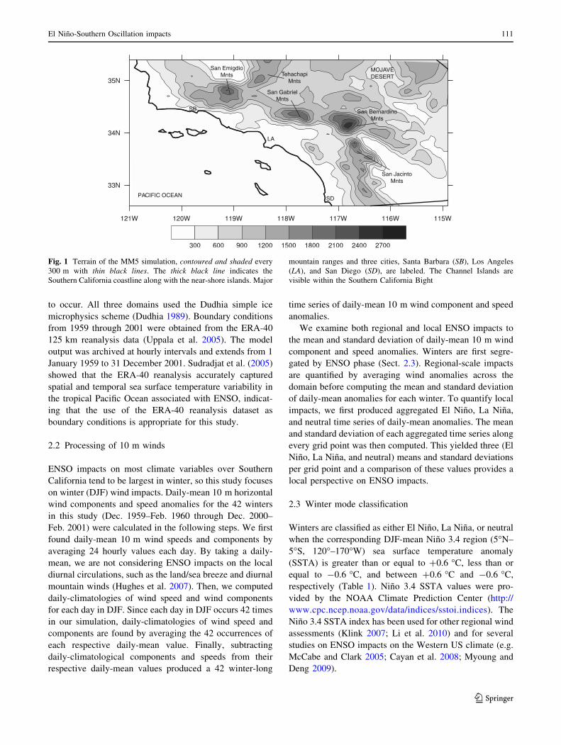
Fig. 1 Terrain of the MM5 simulation, contoured and shaded every
300 m with thin black lines. The thick black line indicates the
Southern California coastline along with the near-shore islands. Major
mountain ranges and three cities, Santa Barbara (SB), Los Angeles
(LA), and San Diego (SD), are labeled. The Channel Islands are
visible within the Southern California Bight
El Nino-Southern Oscillation impacts 111
123

2.4 Model validation
General validation of this simulation’s ability to capture the
spatial and temporal structures of wind variability in
Southern California with reasonable accuracy has been
demonstrated in several previous studies. In Conil and Hall
(2006), an average correlation of 0.7 was found between
hourly model outputs and observations of daily-mean,
near-surface wind direction anomalies for data at 16 land
stations and two ocean buoys within the 6 km resolution
domain. The same study also found correlations above 0.6
between simulated and observed daily-mean, near-surface
wind speed anomalies for 10 locations. Hughes et al.
(2007) further demonstrated agreement between simulated
and observed August wind cycles at 30 locations. Addi-
tional validation was presented in Hughes and Hall (2010),
where correlations between the observed and simulated
daily offshore surface wind component were greater than
0.4 at 37 of the available 42 locations and greater than 0.7
for 13 locations. These previous validation exercises all
provide confidence that the MM5 simulated winds used in
the present study are reasonably realistic.
We undertook more specific validation of the simula-
tion’s ability to capture the general ENSO signals of near-
surface wintertime winds at 25 locations with available data
over Southern California (Fig. 2). Though this observa-
tional network is very sparse, especially in light of the
complex topography and coastline in the region, it is still
possible to draw some conclusions about the quality of the
simulation. At each of the 25 locations, we calculate the
average El Nino minus La Nina difference in the mean
daily-mean 10 m wind speed anomalies. Then we regress
these observed differences between the two phases of
interannual variability onto corresponding simulated dif-
ferences at the nearest model grid point. The correlation
coefficient, slope, and y-intercept for this regression exer-
cise is presented in Table 2 (first row). A high and signifi-
cant correlation of 0.62 (p = 0.001) is found, indicating that
the observed and simulated variations in ENSO impacts on
wind speed vary in phase with one another in space. A slope
of 0.94 is found, indicating that the simulated and observed
anomalies are also very similar in magnitude. Finally, a
y-intercept of -0.2 m s-1 is found. Since the range of
values used in this regression exercise spans from approx-
imately -0.5 to ?0.5 m s-1 for both observed and simu-
lated data, this y-intercept is virtually indistinguishable
from zero, indicating little or no systematic bias in the
simulated ENSO-related wind anomalies.
The model also captures the ENSO impacts on wind
variability, though not quite as well. The second row of
Table 2 shows the results when the average observed El
Nino minus La Nina difference in the mean daily-mean
10 m wind speed standard deviation is regressed onto the
corresponding simulated values. In this case, we find a
slightly weaker but still positive and significant correlation
of 0.46 (p = 0.022). The slope (0.57) is less than one,
suggesting the model may over simulate the spatial varia-
tions in ENSO impacts on wind variability by roughly
50 %. However, the y-intercept is approximately zero
(-0.02) relative to the range of values spanned by the data
(-0.5 to ?0.5 m s-1), indicating very little or no system-
atic bias in the magnitudes of the anomalies.
In addition to the general validation exercises presented in
Fig. 2 and Table 2, we also demonstrate in Fig. 4 that our
simulation is able to capture the temporal changes in average
wind speeds and wind speed variability. Shown in Fig. 4 are
time series of the mean and standard deviation of 10-m daily-
mean wind speed anomalies averaged across the 25 obser-
vations (dashed line) and across the model grid points
nearest to the observation locations (thin black line). Large
and significant correlations between these time series
(r = 0.79, p \ 0.001 for the mean and r = 0.88, p \ 0.001
for the standard deviation) indicate that our simulation is
accurately capturing temporal fluctuations in near-surface
winds over Southern California. Also shown in Fig. 4 are
time series of domain-averaged mean and standard deviation
of 10-m daily-mean winds (thick blank line). The relation-
ship between this time series and ENSO will be discussed in
Sect. 3. Here we simply note that high correlations between
the domain-averaged and observed time series (r = 0.70,
p \ 0.001 in the mean and r = 0.64, p \ 0.001 in the stan-
dard deviation) demonstrate that the sparse network of
observations available for use in this study are in fact well-
representative of the domain as a whole.
Table 1 The classification of winters based on the DJF-mean Nino 3.4 sea surface temperature anomaly
El Nino winters Neutral winters La Nina winters
1964, 1966, 1969, 1970 1960, 1961, 1962, 1967, 1963, 1965, 1968, 1971,
1973, 1983, 1987, 1988, 1975, 1977, 1978, 1979, 1972, 1974, 1976,
1992, 1995, 1998 1980, 1981, 1982, 1990, 1984, 1985, 1986, 1989,
1991, 1993, 1994, 1997 1996, 1999, 2000, 2001
The year of each winter is composed of December of the previous year and January and February of the current year, e.g. 1992 includes
December 1991, January and February 1992
112 N. Berg et al.
123

Before presenting ENSO impacts on surface circulation,
we first confirm in Fig. 3 that the simulation we analyze
reproduces ENSO impacts on precipitation already found
in previous studies (Sect. 1). Compared to neutral winters,
92 % of the Southern California region experiences more
precipitation during El Nino winters. Nearly the entire
region experiences less precipitation during La Nina win-
ters (Fig. 3a). These results are consistent with those of
Redmond and Koch 1991; Dettinger et al. 1998; Cayan
et al. 1999; Leung et al. 2003. Similar to the mean pre-
cipitation signal, increased precipitation variability is
experienced across 64 % of the region during El Nino
(Fig. 3b). This reflects increased extreme precipitation
events during El Nino (Cayan et al. 1999).
3 ENSO impacts on the mean and standard deviation
of winds
Figure 4 shows time series of the mean and standard
deviation of daily-mean 10 m wind speed anomalies for 42
winters (Dec. 1959–Feb. 1960 through Dec. 2000–Feb.
2001). To provide a regional-scale perspective, wind
speeds were averaged over the domain (Fig. 1) before
computing the mean and standard deviation. A signal of
increased variability during El Nino events is evident in the
standard deviation time series. Four of the five highest
standard deviations (1983, 1969, 1998, 1988) happen dur-
ing El Nino winters. Within the highest tercile of standard
deviations, six occur in El Nino conditions. This means that
more than half of all El Nino standard deviations are
located in the highest tercile. Amongst the five lowest
standard deviations, none are found during El Nino. An
opposite variability signal, and one nearly as strong, is also
found for the La Nina phase. Four of the five lowest
standard deviations are recorded during La Nina winters
(1976, 1968, 1986, 1996). None of the five highest standard
deviations occur during La Nina. Seven standard deviations
associated with La Nina years, or slightly less than half of
all La Ninas, occur in the lowest tercile.
Figure 4 also reveals that higher wind variability is
generally accompanied by higher mean winds, and vice
versa. In fact, there is a significant positive correlation
(r = 0.46, p = 0.002) between the mean and standard
deviation time series. This relationship may be orchestrated
in part by the ENSO phenomenon, though previous studies
have shown that a tight correlation between the mean and
standard deviation time series is typical for positively
defined variables, such as wind speed (Jimenez et al. 2008)
and precipitation (Xoplaki et al. 2004). Four of the top five
(1998, 1973, 1969, 1964) and half of the ten highest means
are during El Nino winters. Two of five lowest means also
occur during El Nino winters (1995, 1970). However,
unlike the variability case where an opposite La Nina
signal is found, no clear La Nina signal is seen in the time
series of the means. For example, six means corresponding
to La Nina years are found in both the lowest and middle
terciles.
A more local view of ENSO’s wind impacts is presented
in Fig. 5. This figure shows distributions of the average
R1
R3
R2
Fig. 2 Location of 25 land observations (black dots) along with terrain as in Fig. 1 and the location of three sub-regions (R1, R2, R3) discussed
in the text. Observations are provided by the National Climatic Data Center
Table 2 Correlation coefficient (r), slope (m), and y-intercept (y-int,
m s-1) of the regression line between observed and simulated average
El Nino minus La Nina differences in the mean and standard devia-
tion (stdv) of 10 m daily-mean wind speed anomalies
r m y-int
Mean 0.62 0.94 -0.2
Stdv 0.46 0.57 -0.02
Observation locations are shown in Fig. 2
El Nino-Southern Oscillation impacts 113
123

differences in the mean and standard deviation of daily-
mean wind speed anomalies at each grid point for all El
Nino and La Nina winters compared to neutral winters. The
most striking differences are seen in the standard deviation
signal (Fig. 5b). During El Nino, 78 % of the domain typ-
ically experiences increased wind speed variability. This is
greater than the portion of the domain that experiences
increased precipitation variability during El Nino (64 %,
Fig. 3b). During La Nina, a majority of the domain (66 %)
experiences decreased variability. Higher average wind
speeds are typically experienced over 65 % of the domain
during El Nino (Fig. 5a). Meanwhile, 79 % of the domain
experiences lower average speeds during La Nina. These
ENSO signals in average wind speed are weaker than the
corresponding precipitation signals, as 92 % of the domain
experiences increased precipitation on average during El
Nino and nearly the entire domain experiences decreased
precipitation on average during La Nina (Fig. 3a).
Figure 6 shows maps of the average differences in the
mean and standard deviation of the daily-mean 10 m wind
speed anomalies between the ENSO phases. We will dis-
cuss these maps further in the next section. Here we simply
note that, consistent with the regionally-averaged time
series (Fig. 4) and local summary (Fig. 5) of the ENSO
impacts, increased mean and variability are seen at most
locations when averaged over all El Nino winters (Fig. 6a,
c), while decreased mean and variability are generally seen
when averaged over all La Nina winters (Fig. 6b, d). These
results are all consistent with the hypothesis presented in
the Introduction. A stronger and southward displaced jet
stream and storm track delivers faster winds and more
storms during El Nino. This leads to increased mean wind
speeds and increased wind speed variability across the
region. Conversely, a weaker and northward displaced jet
stream and storm track results in weaker and less variable
wind speeds during La Nina.
4 Spatial structure and relation to large-scale
circulation
The spatial structures of Fig. 6 may be understood by
examining changes in the main wintertime wind regimes of
(a) (b)Fig. 3 Distributions of the
average grid point differences in
mean (a) and standard deviation
(b) of daily-mean precipitation
anomalies between La Nina and
neutral winters (blue) and El
Nino and neutral winters (red)
over the simulated Southern
California region
Fig. 4 Time series showing the mean and standard deviation of 10-m
daily-mean wind speed anomalies for each simulated winter. Values
are spatially-averaged across the entire domain (thick black line),
across all grid points nearest to the observation locations (thin blackline), and across all observations (dashed line). Red dots indicate El
Nino winters and blue dots indicate La Nina winters. Unit for each
time series is m s-1
114 N. Berg et al.
123

Southern California, which are classified using a cluster
analysis technique. Conil and Hall (2006) applied this same
technique to a 10-year long subset of the time series used in
this paper, and provide details about the technique itself.
When it is applied to the 42-winter time series, the results
are very similar. Here we briefly summarize these results,
and refer the reader to Conil and Hall (2006) for further
information.
(a) (b)Fig. 5 Distributions of the
average grid point differences in
mean (a) and standard deviation
(b) of daily-mean 10 m wind
speed anomalies between La
Nina and neutral winters (blue)
and El Nino and neutral winters
(red) over the simulated
Southern California region
(a) (b)
(d)(c)
Fig. 6 Average differences of the mean and standard deviation (stdv)
for daily-mean 10 m wind speed anomalies between El Nino (a,
c) and La Nina (b, d) winters compared to neutral winters. Contour
interval is 0.1. Positive differences are shaded red and negative
differences are shaded blue. Regions of significant differences (at the
90 % level using the t test) are hatched. The domain-averaged value is
reported on the top right of each plot. Unit for each plot is m s-1
El Nino-Southern Oscillation impacts 115
123
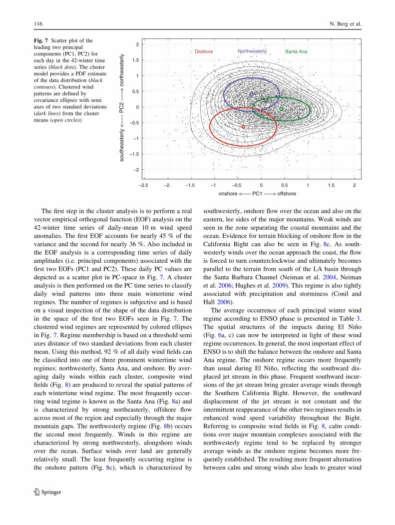
The first step in the cluster analysis is to perform a real
vector empirical orthogonal function (EOF) analysis on the
42-winter time series of daily-mean 10 m wind speed
anomalies. The first EOF accounts for nearly 45 % of the
variance and the second for nearly 36 %. Also included in
the EOF analysis is a corresponding time series of daily
amplitudes (i.e. principal components) associated with the
first two EOFs (PC1 and PC2). These daily PC values are
depicted as a scatter plot in PC-space in Fig. 7. A cluster
analysis is then performed on the PC time series to classify
daily wind patterns into three main wintertime wind
regimes. The number of regimes is subjective and is based
on a visual inspection of the shape of the data distribution
in the space of the first two EOFs seen in Fig. 7. The
clustered wind regimes are represented by colored ellipses
in Fig. 7. Regime membership is based on a threshold semi
axes distance of two standard deviations from each cluster
mean. Using this method, 92 % of all daily wind fields can
be classified into one of three prominent wintertime wind
regimes: northwesterly, Santa Ana, and onshore. By aver-
aging daily winds within each cluster, composite wind
fields (Fig. 8) are produced to reveal the spatial patterns of
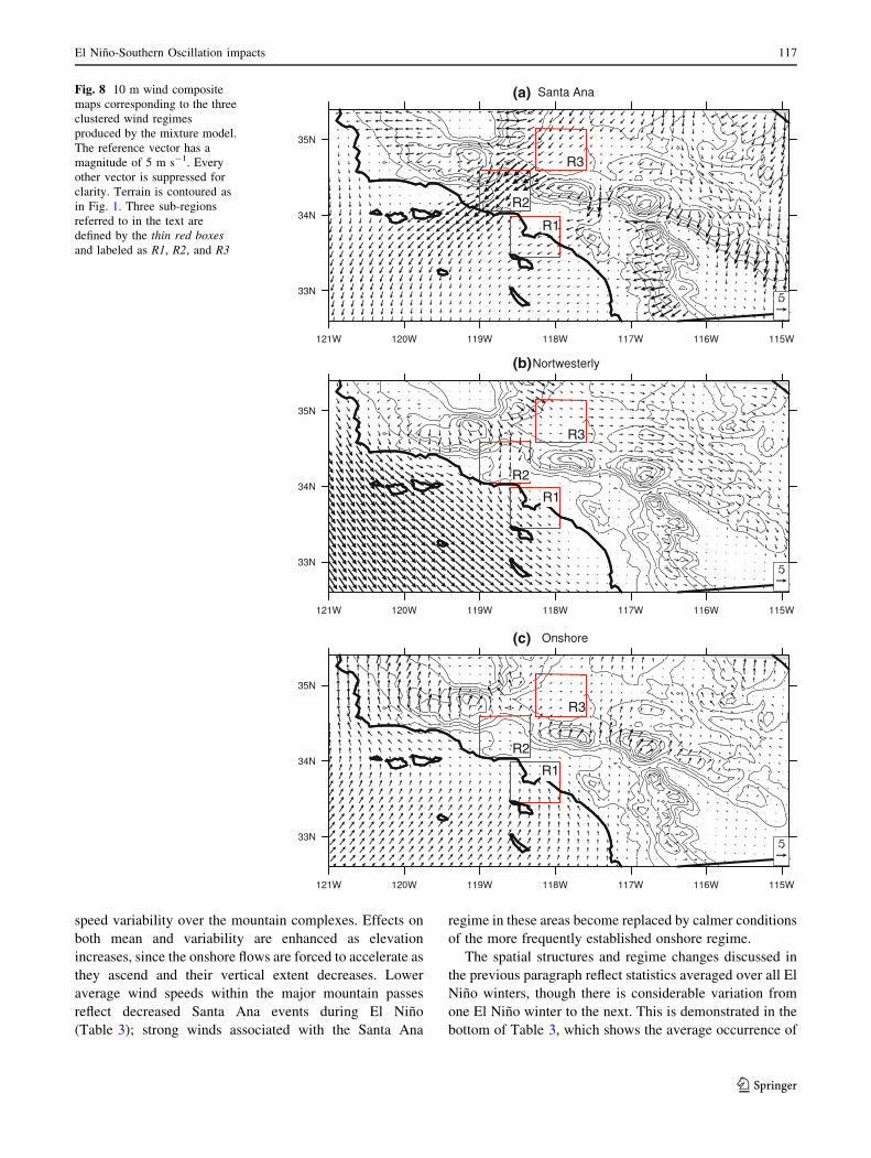
each wintertime wind regime. The most frequently occur-
ring wind regime is known as the Santa Ana (Fig. 8a) and
is characterized by strong northeasterly, offshore flow
across most of the region and especially through the major
mountain gaps. The northwesterly regime (Fig. 8b) occurs
the second most frequently. Winds in this regime are
characterized by strong northwesterly, alongshore winds
over the ocean. Surface winds over land are generally
relatively small. The least frequently occurring regime is
the onshore pattern (Fig. 8c), which is characterized by
southwesterly, onshore flow over the ocean and also on the
eastern, lee sides of the major mountains. Weak winds are
seen in the zone separating the coastal mountains and the
ocean. Evidence for terrain blocking of onshore flow in the
California Bight can also be seen in Fig. 8c. As south-
westerly winds over the ocean approach the coast, the flow
is forced to turn counterclockwise and ultimately becomes
parallel to the terrain from south of the LA basin through
the Santa Barbara Channel (Neiman et al. 2004, Neiman
et al. 2006; Hughes et al. 2009). This regime is also tightly
associated with precipitation and storminess (Conil and
Hall 2006).
The average occurrence of each principal winter wind
regime according to ENSO phase is presented in Table 3.
The spatial structures of the impacts during El Nino
(Fig. 6a, c) can now be interpreted in light of these wind
regime occurrences. In general, the most important effect of
ENSO is to shift the balance between the onshore and Santa
Ana regime. The onshore regime occurs more frequently
than usual during El Nino, reflecting the southward dis-
placed jet stream in this phase. Frequent southward incur-
sions of the jet stream bring greater average winds through
the Southern California Bight. However, the southward
displacement of the jet stream is not constant and the
intermittent reappearance of the other two regimes results in
enhanced wind speed variability throughout the Bight.
Referring to composite wind fields in Fig. 8, calm condi-
tions over major mountain complexes associated with the
northwesterly regime tend to be replaced by stronger
average winds as the onshore regime becomes more fre-
quently established. The resulting more frequent alternation
between calm and strong winds also leads to greater wind
−2.5 −2 −1.5 −1 −0.5 0 0.5 1 1.5 2
−2
−1.5
−1
−0.5
0
0.5
1
1.5
2
onshore <−−− PC1 −−−> offshore
sout
heas
terly
<−
−−
PC
2 −
−−
> n
orth
wes
terly
Onshore Northwesterly Santa Ana
Fig. 7 Scatter plot of the
leading two principal
components (PC1, PC2) for
each day in the 42-winter time
series (black dots). The cluster
model provides a PDF estimate
of the data distribution (blackcontours). Clustered wind
patterns are defined by
covariance ellipses with semi
axes of two standard deviations
(dark lines) from the cluster
means (open circles)
116 N. Berg et al.
123
speed variability over the mountain complexes. Effects on
both mean and variability are enhanced as elevation
increases, since the onshore flows are forced to accelerate as
they ascend and their vertical extent decreases. Lower
average wind speeds within the major mountain passes
reflect decreased Santa Ana events during El Nino
(Table 3); strong winds associated with the Santa Ana
regime in these areas become replaced by calmer conditions
of the more frequently established onshore regime.
The spatial structures and regime changes discussed in
the previous paragraph reflect statistics averaged over all El
Nino winters, though there is considerable variation from
one El Nino winter to the next. This is demonstrated in the
bottom of Table 3, which shows the average occurrence of
R1
R2
R3
R1
R2
R3
R1
R2
R3
(a)
(b)
(c)
Fig. 8 10 m wind composite
maps corresponding to the three
clustered wind regimes
produced by the mixture model.
The reference vector has a
magnitude of 5 m s-1. Every
other vector is suppressed for
clarity. Terrain is contoured as
in Fig. 1. Three sub-regions
referred to in the text are
defined by the thin red boxesand labeled as R1, R2, and R3
El Nino-Southern Oscillation impacts 117
123

each principal wind regime for the three strongest El Nino
winters. Especially strong signals of both increased
onshore events and decreased Santa Ana events can been
seen during these large El Nino events. For example, while
the average increase in onshore events during El Nino
winters is approximately 20 % compared to neutral con-
ditions, the El Nino winter of 1992 experienced nearly
70 % more onshore events. Another example is seen in the
winter of 1998, which experienced over 55 % fewer Santa
Ana events, while the average reduction in Santa Ana
events during El Nino is roughly 20 %.
The results in Table 3 also help to explain the spatial
structures of the La Nina impacts (Fig. 6b, d). During La
Nina conditions, the northwesterly regime occurs more
frequently than usual at the expense of the onshore regime.
This leads to slightly greater winds over the western half of
the Southern California Bight and significantly weaker
winds over the eastern half of the Bight and coastal basin, as
seen in Fig. 8. Since the onshore regime occurs less fre-
quently during La Nina, lower variability is found in much
of the Southern California Bight and over the mountain
complexes, i.e. the regions that correspond to higher vari-
ability during El Nino (Fig. 6c, d). Greater variability along
prominent mountain passes during La Nina is also tied to a
reduction of onshore events. Winds in the passes are very
weak during an onshore event. With fewer onshore events
during La Nina, alternations between strong winds of the
Santa Ana regime and the weak winds of the northwesterly
regime become more frequent. This vacillation likely leads
to increased wind speed variability in the passes.
Three sub-regions (see Fig. 8) are selected to explore
the local implications of the spatial structures in ENSO
impacts seen in Fig. 6. Each sub-region is defined as a ten
grid point by ten grid point domain (60 km by 60 km).
Figure 9 shows average differences in the mean and stan-
dard deviation of wind speed for all El Nino and La Nina
winters compared to neutral winters over the three sub-
regions. We also average the wind magnitudes seen in
Fig. 8 across each sub-region, and present the resulting
values for each regime in Table 4. These typical wind
speeds occurring during each regime, together with the
ENSO-induced changes in the regimes seen in Table 3, can
be used to develop qualitative explanations for the origins
of the various ENSO signals in each sub-region.
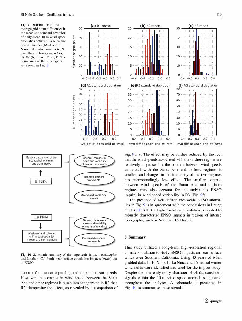
The first sub-region, ‘‘R1’’, shows an ENSO signal that
is similar to the domain-averaged signal, yet even more
pronounced (Fig. 4). Nearly all grid points in R1 experi-
ence increased mean speeds and wind speed variability
during El Nino and decreased mean speeds and variability
during La Nina (Fig. 9a, d). This may be related to the
ENSO-induced shift in the frequency of the onshore and
Santa Ana regimes. The onshore regime has relatively large
wind anomalies in this sub-region’s unsheltered, coastal
location, while Santa Ana wind anomalies are very small in
this sub-region. Thus, decreased frequency of the Santa
Ana regime and increased frequency of the onshore regime
during El Nino probably increases both mean winds and
wind variability (Tables 3, 4; Fig. 8).
The second sub-region, ‘‘R2’’, which covers much of the
southern side of the San Emigdio Mountains, experiences a
strong ENSO signal, but one that is opposite to the domain-
averaged ENSO signal. Most grid points within R2 experience
increased wind speed variability during La Nina (Fig. 9e).
Meanwhile, decreased mean speeds and wind speed vari-
ability is seen over a majority of R2 during El Nino (Fig. 9b,
e). These opposite signals in R2 may reflect two factors, based
on evidence seen in Tables 3 and 4 and Fig. 8b, c: (1) The
onshore regime has rather weak wind anomalies in this sub-
region, so that greater frequency of the onshore regime during
El Nino does not lead to great wind speeds or wind variability,
and (2) The Santa Ana regime has very strong wind anomalies
in this region, so that reduced occurrence of Santa Ana winds
during El Nino has the effect of reducing both mean winds and
wind variability. Given the very large magnitude of the winds
during the Santa Ana regime in this sub-region, the later factor
may be the most important.
We next turn to ENSO signals in the third sub-region,
‘‘R3’’, located south of the Tehachipi Mountains and
including the Tehachipi Pass Wind Farm (35.06�N,
118.16�W). The ENSO impact on average winds is quali-
tatively similar to that seen in R2, with nearly half of R3
experiencing decreases in the mean during El Nino
(Fig. 9c). As with R2, the average wind speed during the
Santa Ana regime is relatively high (Table 4), and the
reduction in Santa Ana frequency during El Nino may
Table 3 Average occurrence of each principal wind regime (days per
winter) according to ENSO phase (top) and actual occurrence of each
principal wind regime (days) during the three strongest El Nino
winters (bottom)
Santa Ana Northwesterly Onshore
El Nino 31 33 18
Neutral 37 32 15
La Nina 35 37 13
1983 31 33 20
1998 16 39 20
1992 35 24 25
Table 4 Average wind speed (m s-1) of each principal wind regime
within three sub-regions, R1, R2, and R3
Santa Ana Northwesterly Onshore
R1 1.79 2.25 1.92
R2 6.09 2.53 1.15
R3 2.69 1.75 1.48
118 N. Berg et al.
123
account for the corresponding reduction in mean speeds.
However, the contrast in wind speed between the Santa
Ana and other regimes is much less exaggerated in R3 than
R2, dampening the effect, as revealed by a comparison of
Fig. 9b, c. The effect may be further reduced by the fact
that the wind speeds associated with the onshore regime are
relatively large, so that the contrast between wind speeds
associated with the Santa Ana and onshore regimes is
smaller, and changes in the frequency of the two regimes
has correspondingly less effect. The smaller contrast
between wind speeds of the Santa Ana and onshore
regimes may also account for the ambiguous ENSO
imprint in wind speed variability in R3 (Fig. 9f).
The presence of well-defined mesoscale ENSO anoma-
lies in Fig. 9 is in agreement with the conclusions in Leung
et al. (2003) that a high-resolution simulation is needed to
robustly characterize ENSO impacts in regions of intense
topography, such as Southern California.
5 Summary
This study utilized a long-term, high-resolution regional
climate simulation to study ENSO impacts on near-surface
winds over Southern California. Using 43 years of 6 km
gridded data, 11 El Nino, 15 La Nina, and 16 neutral winter
wind fields were identified and used for the impact study.
Despite the inherently noisy character of winds, consistent
signals within the 10 m wind speed anomalies appeared
throughout the analyses. A schematic is presented in
Fig. 10 to summarize these signals.
(a) (b) (c)
(f)(e)(d)
Fig. 9 Distributions of the
average grid point differences in
the mean and standard deviation
of daily-mean 10 m wind speed
anomalies between La Nina and
neutral winters (blue) and El
Nino and neutral winters (red)
over three sub-regions, R1 (a,
d), R2 (b, e), and R3 (c, f). The
boundaries of the sub-regions
are shown in Fig. 8
El Niño
La Niña
Eastward extension of the subtropical jet stream
and storm tracks
General increase inmean and variability
of near-surface winds
Westward and polewardshift in subtropical jet
stream and storm stracks
Increased onshoreflow events
Decreased Santa Ana events
General decrease inmean and variability
of near-surface winds
Decreased onshoreflow events
Fig. 10 Schematic summary of the large-scale impacts (rectangles)
and Southern California near-surface circulation impacts (ovals) due
to ENSO
El Nino-Southern Oscillation impacts 119
123

In response to the equatorward and eastward extension
of the subtropical jet stream and storm tracks in the
Northern Hemisphere, Southern California experiences
general increases in average wind speed and wind speed
variability during El Nino. More than half of the Southern
California region experiences increased mean wind speeds
during El Nino, while nearly 80 % of the region experi-
ences increased wind speed variability. The El Nino signal
of increased wind speed variability is experienced over a
larger portion of Southern California than the correspond-
ing signal of increased precipitation variability. Con-
versely, a westward and poleward shift to the jet stream
and storm tracks during La Nina leads to general decreases
in the mean and variability of winds over Southern Cali-
fornia. A majority of the Southern California region
experiences decreased wind speed variability during La
Nina events. Similarly, more than half of the region
experiences reduced average wind speeds during La Nina,
though this signal is not seen in the regionally-averaged
time series of mean winter wind speeds. It should be noted,
however, that our model captures the ENSO impacts on
mean winds better than impacts on wind variability.
Daily winter wind fields were classified into three main
wintertime wind regimes, northwesterly, Santa Ana, and
onshore through a classification technique known as a
cluster analysis. This analysis revealed shifts in the fre-
quency of main wintertime wind regimes based on ENSO
phase. It is found that the onshore regime occurs more
frequently during El Nino and occurs less frequently during
La Nina. Meanwhile, the Santa Ana regime occurs some-
what less frequently during El Nino. Over land, shifts in
occurrences of the onshore and Santa Ana regimes lead to
significant mesoscale spatial structures with a strong
topographic imprint during both phases. Increased onshore
events during El Nino, at the expense of the Santa Ana
regime, leads to greater winds and wind variability across
the Southern California Bight and weaker winds in
mountain passes where Santa Ana-like outflow is typically
found. Reduced Santa Ana events also help explain
decreased average wind speeds within the major mountain
passes. Strong outflow through these regions associated
with the Santa Ana regime becomes replaced by weaker
winds of the more frequently occurring onshore regime.
During La Nina, the onshore regime occurs less frequently
than usual with corresponding higher occurrences of the
northwesterly regime. This likely explains lower average
wind speeds and wind speed variability through much of
the coastal zone. Reduced onshore events yield increased
vacillation between strong Santa Ana winds and weak
northwesterly winds within major mountain passes, and
increased wind variability in these regions during La Nina.
The major findings in this study imply that ENSO likely
can significantly impact wind power production over
Southern California. As such, we believe this study moti-
vates further analyses that quantify ENSO impacts on wind
speeds at heights appropriate to wind power generation.
Such analyses would help the wind power industry plan for
interannual variations in wind power and potentially pre-
dict wind power anomalies based on ENSO predictions.
Acknowledgments This work was funded by a grant to the Los
Angeles Regional Collaborative by the US Department of Energy
through the City and County of Los Angeles. We thank two anony-
mous reviewers for their constructive criticism of this manuscript.
References
Cayan DR, Redmond KT, Riddle LG (1999) ENSO and hydrologic
extremes in the Western United States. J Clim 12:2881–2893
Cayan DR, Bromirski PD, Hayhoe K, Tyree M, Dettinger MD, Flick
RE (2008) Climate change projections of sea level extremes
along the California coast. Clim Change 87:57–73
Chen WY, van den Dool HM (1997) Asymmetric impact of tropical
SST anomalies on atmospheric internal variability over the
North Pacific. J Atmos Sci 54:725–740
Conil S, Hall A (2006) Local regimes of atmospheric variability: a
case study of Southern California. J Clim 19:4308–4325
Dettinger MD, Cayan DR, Diaz HF, Meko DM (1998) North-south
precipitation patterns in Western North America on interannual-
to-decadal timescales. J Clim 11:3095–3111
Dudhia J (1989) Numerical study of convection observed during the
winter monsoon experiment using a mesoscale two-dimensional
model. J Atmos Sci 46:3077–3107
Dvorak MJ, Archer CL, Jacobson MZ (2010) California offshore
wind energy potential. Renew Energy 35:1244–1254
Enloe J, O’Brien JJ, Smith SR (2004) ENSO impacts on peak wind
gusts in the United States. J Clim 17:1728–1737
George S, Wolfe SA (2009) El Nino stills winter winds across the
southern Canadian Prairies. Geophys Res Lett 36:1–5
Grell GA, Dudhia J, Stauffer DR (1994) A description of the fifth-
generation Penn State/NCAR Mesoscale Model (MM5). Tech-
nical report NCAR Tech. Note NCAR/TN 398?STR
Held IM, Lyons SW, Nigam S (1989) Transients and the extratropical
response to El Nino. J Atmos Sci 46:163–174
Hughes M, Hall A (2010) Local and synoptic mechanisms causing
Southern California’s Santa Ana winds. Clim Dyn 34:847–857
Hughes M, Hall A, Fovell RG (2007) Dynamical controls on the
diurnal cycle of temperature in complex topography. Clim Dyn
29:277–292
Hughes M, Hall A, Fovell RG (2009) Blocking in areas of complex
topography, and its influence on rainfall distribution. J Atmos Sci
66:508–518
Jiang Q, Doyle JD, Haack T, Dvorak MJ, Archer CL, Jacobson MZ
(2008) Exploring wind energy potential off the California coast.
Geophys Res Let 35:L20819
Jimenez PA, Gonzalez-Rouco JF, Montavez JP, Navarro J, Garcia-
Bustamante E, Valdero F (2008) Surface wind regionalization in
complex terrain. J Appl Meteor Climatol 47:308–325
Kain JS (2002) The Kain–Fritsch convective parameterization: an
update. J of Appl Meteor 43:170–181
Klink K (2007) Atmospheric circulation effects on wind speed
variability at turbine height. J Appl Meteor Climatol 46:445–456
Leung LR, Qian Y, Bian X, Hunt A (2003) Hydroclimate of the
Western United States based on observations and regional
climate simulation of 1981–2000. Part II: mesoscale ENSO
anomalies. J Clim 16:1912–1928
120 N. Berg et al.
123

Li X, Zhong S, Bian X, Heilman WE (2010) Climate and climate
variability of the wind power resources in the Great Lakes region
of the United States. J Geophys Res 115:1–15
McCabe GJ, Clark MP (2005) Trends and variability in snowmelt
runoff in the Western United States. J Hydrometeor 6:476–482
Myoung B, Deng Y (2009) Interannual variability of the cyclonic
activity along the U.S. Pacific Coast: influences on the charac-
teristics of winter precipitation in the Western United States.
J Clim 22:5732–5747
Neiman PJ, Persson POG, Ralph FM, Jorgensen DP, White AB,
Kingsmill DE (2004) Modification of fronts and precipitation by
coastal blocking during an intense landfalling winter storm in
Southern California: observations during CALJET. Mon Wea
Rev 132:242–273
Neiman PJ, Ralph FM, White AB, Parrish DD, Holloway JS, Bartels
DL (2006) A multiwinter analysis of channeled flow through a
prominent gap along the Northern California coast during
CALJET and PACJET. Mon Wea Rev 134:1815–1841
Redmond KT, Koch RW (1991) Surface climate and streamflow
variability in the Western United States and their relationship to
large-sale circulation indices. Water Resour Res 27:2381–2399
Shabbar A (2006) The impact of El Nino-Southern Oscillation on the
Canadian climate. Adv In Geosci 6:149–153
Straus DM, Shukla J (1997) Variations of midlatitude transient
dynamics associated with ENSO. J Atmos Sci 54:777–790
Sudradjat A, Ferraro RR, Fiorino M (2005) A comparison of total
precipitable water between reanalyses and NVAP. J Clim
18:1790–1807
Trenberth KE, Hurrell JW (1994) Decadal atmosphere-ocean varia-
tions in the Pacific. Clim Dyn 9:303–319
Uppala SM et al (2005) The ERA-40 reanalysis. Q J R Meteorol Soc
131:2961–3012
Xoplaki E, Gonzalez-Rouco JF, Luterbacker J, Wanner H (2004) Wet
season Mediterranean precipitation variability: influence of
large-scale dynamics and trends. Clim Dyn 23:63–78
El Nino-Southern Oscillation impacts 121
123


