
EFFICIENT ALGORITHMS FOR COMPUTATIONS
WITH SPARSE POLYNOMIALS
by
Seyed Mohammad Mahdi Javadi
B.Sc., Sharif University of Technology, 2004
M.Sc., Simon Fraser University, 2006
a Thesis submitted in partial fulfillment
of the requirements for the degree of
Doctor of Philosophy
in the School
of
Computing Science
c© Seyed Mohammad Mahdi Javadi 2011
SIMON FRASER UNIVERSITY
Spring 2011
All rights reserved. This work may not be
reproduced in whole or in part, by photocopy
or other means, without the permission of the author.

APPROVAL
Name: Seyed Mohammad Mahdi Javadi
Degree: Doctor of Philosophy
Title of Thesis: Efficient Algorithms for Computations with Sparse Polyno-
mials
Examining Committee: Dr. Valentine Kabanets
Chair
Dr. Michael Monagan, Senior Supervisor
Dr. Arvind Gupta, Supervisor
Dr. Marni Mishna, SFU Examiner
Dr. Mark Giesbrecht, External Examiner
Date Approved:
ii

Abstract
The problem of interpolating a sparse polynomial has always been one of the central objects
of research in the area of computer algebra. It is the key part of many algorithms such as
polynomial GCD computation. We present a probabilistic algorithm to interpolate a sparse
multivariate polynomial over a finite field, represented with a black box. Our algorithm
modifies the Ben-Or/Tiwari algorithm from 1988 for interpolating polynomials over rings
with characteristic zero to positive characteristics by doing additional probes. To interpo-
late a polynomial in n variables with t non-zero terms, Zippel’s algorithm interpolates one
variable at a time using O(ndt) probes to the black box where d bounds the degree of the
polynomial. Our new algorithm does O(nt) probes. We provide benchmarks comparing our
algorithm to Zippel’s algorithm and the racing algorithm of Kaltofen/Lee. The benchmarks
demonstrate that for sparse polynomials our algorithm often makes fewer probes. A key
advantage in our new algorithm is, unlike the other two algorithms, it can be parallelized
efficiently.
Our main application for an efficient sparse interpolation algorithm is computing GCDs
of polynomials. We are especially interested in polynomials over algebraic function fields.
The best GCD algorithm available is SparseModGcd, presented by Javadi and Monagan
in 2006. We further improve this algorithm in three ways. First we prove that we can
eliminate the trial divisions in positive characteristic. Trial divisions are the bottleneck
of the algorithm for denser polynomials. Second, we give a new (and correct) solution to
the normalization problem. Finally we will present a new in-place library of functions for
computing GCDs of univariate polynomials over algebraic number fields.
Furthermore we present an efficient algorithm for factoring multivariate polynomials over
algebraic fields with multiple field extensions and parameters. Our algorithm uses Hensel
lifting and extends the EEZ algorithm of Wang which was designed for factorization over
iii

rationals. We also give a multivariate p-adic lifting algorithm which uses sparse interpola-
tion. This enables us to avoid using poor bounds on the size of the integer coefficients in the
factorization when using Hensel lifting. We provide timings demonstrating the efficiency of
our algorithm.
iv

To my beloved wife, Maryam,
and my wonderful son, Ali,
and my dearest parents, Nahid and Ahmad
v

ÕækQË@ á
Ô gQË@ é
<Ë@ Õæ
.
vi

Acknowledgments
My foremost gratitude goes to my wonderful adviser, Michael Monagan, whose invaluable
guidance and generous support has always been with me during my Ph.D. studies at SFU.
It was a real pleasure for me to do my Ph.D. with him. His continuous encouragement and
belief in me were vital in the advancement of my graduate career. I’m especially thankful
to Mike for being constantly available for discussions that would always lead to new ideas,
thoughts, and insights. For all this and more, I gratefully thank him.
I also thank the members of my thesis committee: Mark Giesbrecht, Arvind Gupta,
Marni Mishna and Valentine Kabanets for reading my thesis, being present at my defence
session and providing me with many feedbacks.
I also take this opportunity to thank one of my best friends at SFU, Roman Pearce. We
had many, many wonderful discussions about computer algebra and most importantly life!
He taught me a great deal about his fascinating work on Maple. We were on several trips
together. I will never forget our several hours of walking in Seoul. Thank you Roman!
I’d like to extend my warmest gratitude to one of my best and most brilliant friends;
Roozbeh Ghaffari for being so amazingly caring, kind and supportive. Roozbeh has un-
doubtedly been one of the most influential people in my life. Thank you Roozbeh!
Finally, I am deeply thankful to my family for all the things they have done for me. I
am grateful to my parents for their unconditional support, constant encouragement, and
faith in me throughout my whole life. I am also deeply thankful to my beloved wife,
colleague and best friend, Maryam, whose love, help and tolerance exceeded all reasonable
bounds. She made my study easier with love and patience: without her constant support
and encouragement this thesis would have been an impossibility. I should also thank my
lovely son, Ali who always supports me with his little heart!
vii

Contents
Approval ii
Abstract iii
Dedication v
Quotation vi
Acknowledgments vii
Contents viii
List of Tables xi
List of Figures xii
List of Algorithms xiii
1 Introduction 1
1.1 Polynomial Interpolation . . . . . . . . . . . . . . . . . . . . . . . . . . . . . . 3
1.1.1 Zippel’s Algorithm . . . . . . . . . . . . . . . . . . . . . . . . . . . . . 4
1.1.2 Ben-Or/Tiwari Sparse Interpolation Algorithm . . . . . . . . . . . . . 7
1.1.3 Hybrid of Zippel’s and Ben-Or/Tiwari’s Algorithms . . . . . . . . . . 10
1.1.4 Other Sparse Interpolation Algorithms . . . . . . . . . . . . . . . . . . 12
1.2 GCD Computation of Multivariate Polynomials over Z . . . . . . . . . . . . . 14
1.2.1 The Euclidean Algorithm and Polynomial Remainder Sequences . . . 14
1.2.2 The GCDHEU Algorithm . . . . . . . . . . . . . . . . . . . . . . . . . 15
viii

1.2.3 Brown’s Modular GCD Algorithm . . . . . . . . . . . . . . . . . . . . 16
1.2.4 Zippel’s Sparse Interpolation Algorithm . . . . . . . . . . . . . . . . . 19
1.2.5 LINZIP Algorithm and the Normalization Problem . . . . . . . . . . . 20
1.3 Polynomial Factorization . . . . . . . . . . . . . . . . . . . . . . . . . . . . . . 23
1.3.1 The EEZ Algorithm and Hensel Lifting . . . . . . . . . . . . . . . . . 24
1.3.2 Gao’s Algorithm . . . . . . . . . . . . . . . . . . . . . . . . . . . . . . 26
1.3.3 Polynomial Factorization over Algebraic Fields . . . . . . . . . . . . . 26
1.3.4 Trager’s Algorithm . . . . . . . . . . . . . . . . . . . . . . . . . . . . . 27
1.3.5 Other Algorithms . . . . . . . . . . . . . . . . . . . . . . . . . . . . . . 28
1.4 Outline of Thesis . . . . . . . . . . . . . . . . . . . . . . . . . . . . . . . . . . 30
2 Parallel Sparse Interpolation 32
2.1 The Idea and an Example . . . . . . . . . . . . . . . . . . . . . . . . . . . . . 33
2.2 Problems . . . . . . . . . . . . . . . . . . . . . . . . . . . . . . . . . . . . . . 36
2.2.1 Distinct Monomials . . . . . . . . . . . . . . . . . . . . . . . . . . . . 36
2.2.2 Root Clashing . . . . . . . . . . . . . . . . . . . . . . . . . . . . . . . 37
2.3 The Algorithm . . . . . . . . . . . . . . . . . . . . . . . . . . . . . . . . . . . 38
2.3.1 Complexity Analysis . . . . . . . . . . . . . . . . . . . . . . . . . . . . 40
2.3.2 Optimizations . . . . . . . . . . . . . . . . . . . . . . . . . . . . . . . . 42
2.4 Benchmarks . . . . . . . . . . . . . . . . . . . . . . . . . . . . . . . . . . . . . 48
2.5 Comparison of Different Algorithms . . . . . . . . . . . . . . . . . . . . . . . 54
3 GCD Computation 57
3.1 Univariate GCDs over Algebraic Number Fields . . . . . . . . . . . . . . . . . 63
3.1.1 Polynomial Representation . . . . . . . . . . . . . . . . . . . . . . . . 65
3.1.2 In-place Algorithms . . . . . . . . . . . . . . . . . . . . . . . . . . . . 67
3.1.3 Working Space . . . . . . . . . . . . . . . . . . . . . . . . . . . . . . . 74
3.1.4 Benchmarks . . . . . . . . . . . . . . . . . . . . . . . . . . . . . . . . . 77
3.1.5 Remarks . . . . . . . . . . . . . . . . . . . . . . . . . . . . . . . . . . . 80
3.2 Eliminating the Trial Divisions . . . . . . . . . . . . . . . . . . . . . . . . . . 80
3.3 The Normalization Problem . . . . . . . . . . . . . . . . . . . . . . . . . . . . 84
4 Factorization 93
4.1 An Example . . . . . . . . . . . . . . . . . . . . . . . . . . . . . . . . . . . . . 95
ix

4.2 Problems . . . . . . . . . . . . . . . . . . . . . . . . . . . . . . . . . . . . . . 98
4.2.1 The Defect . . . . . . . . . . . . . . . . . . . . . . . . . . . . . . . . . 99
4.2.2 Good and Lucky Evaluation Points . . . . . . . . . . . . . . . . . . . . 100
4.2.3 Degree Bound for the Parameters . . . . . . . . . . . . . . . . . . . . . 103
4.2.4 Numerical Bound . . . . . . . . . . . . . . . . . . . . . . . . . . . . . . 103
4.3 The Algorithm . . . . . . . . . . . . . . . . . . . . . . . . . . . . . . . . . . . 104
4.4 Benchmarks . . . . . . . . . . . . . . . . . . . . . . . . . . . . . . . . . . . . . 112
5 Summary and Future Work 117
Bibliography 120
x

List of Tables
2.1 benchmark #1: n = 3 and D = 30 . . . . . . . . . . . . . . . . . . . . . . . . 50
2.2 benchmark #1: bad degree bound d = 100 . . . . . . . . . . . . . . . . . . . 51
2.3 benchmark #2: n = 3 and D = 100 . . . . . . . . . . . . . . . . . . . . . . . 52
2.4 benchmark #3: n = 6 and D = 30 . . . . . . . . . . . . . . . . . . . . . . . 53
2.5 benchmark #4: n = 12 and D = 30 . . . . . . . . . . . . . . . . . . . . . . . 54
2.6 Parallel speedup timing data for benchmark #4 for an earlier attempt. . . . 55
2.7 Parallel speedup timing data for benchmark #4 for the new algorithm. . . . . 55
2.8 benchmark #5. . . . . . . . . . . . . . . . . . . . . . . . . . . . . . . . . . . . 56
2.9 Comparison of different algorithms. . . . . . . . . . . . . . . . . . . . . . . . . 56
3.1 Timings in CPU seconds on an AMD Opteron 254 CPU running at 2.8 GHz . 78
3.2 Timings (in CPU seconds) for SPARSE-1 . . . . . . . . . . . . . . . . . . . . 92
3.3 Timings (in CPU seconds) for DENSE-1 . . . . . . . . . . . . . . . . . . . . . 92
4.1 Timings (in CPU seconds) . . . . . . . . . . . . . . . . . . . . . . . . . . . . . 116
4.2 Timing (percentile) for different parts of efactor . . . . . . . . . . . . . . . . . 116
xi

List of Figures
1.1 The black box representation . . . . . . . . . . . . . . . . . . . . . . . . . . . 3
2.1 The bipartite graph G1 . . . . . . . . . . . . . . . . . . . . . . . . . . . . . . 43
2.2 Node rkj of graph Gk . . . . . . . . . . . . . . . . . . . . . . . . . . . . . . . 44
2.3 The bipartite graph G1 . . . . . . . . . . . . . . . . . . . . . . . . . . . . . . 45
2.4 The bipartite graph G′1 . . . . . . . . . . . . . . . . . . . . . . . . . . . . . . 46
2.5 The bipartite graph G1 . . . . . . . . . . . . . . . . . . . . . . . . . . . . . . 46
2.6 The bipartite graph G′1 . . . . . . . . . . . . . . . . . . . . . . . . . . . . . . 47
2.7 The bipartite graphs G2 and H2 . . . . . . . . . . . . . . . . . . . . . . . . . 48
xii

List of Algorithms
2.1 Algorithm: Parallel Interpolation . . . . . . . . . . . . . . . . . . . . . . . . . 38
3.1 Zippel’s Modular GCD Algorithm: MGCD . . . . . . . . . . . . . . . . . . . 58
3.2 Zippel’s Modular GCD Algorithm: PGCD . . . . . . . . . . . . . . . . . . . . 58
3.3 Zippel’s Sparse Interpolation Algorithm . . . . . . . . . . . . . . . . . . . . . 59
3.4 Algorithm IP MUL: In-place Multiplication . . . . . . . . . . . . . . . . . . . 68
3.5 Algorithm IP REM: In-place Remainder . . . . . . . . . . . . . . . . . . . . . 69
3.6 Algorithm IP INV: In-place inverse of an element in RN . . . . . . . . . . . . 71
3.7 Algorithm IP GCD: In-place GCD Computation . . . . . . . . . . . . . . . . 73
4.1 Algorithm efactor . . . . . . . . . . . . . . . . . . . . . . . . . . . . . . . . . . 104
4.2 Main Factorization Algorithm . . . . . . . . . . . . . . . . . . . . . . . . . . . 104
4.3 Sparse p-adic lifting . . . . . . . . . . . . . . . . . . . . . . . . . . . . . . . . 106
4.4 Univariate Factorization . . . . . . . . . . . . . . . . . . . . . . . . . . . . . . 107
4.5 Distinct prime divisors (Similar to Wang [77]) . . . . . . . . . . . . . . . . . . 107
4.6 Distributing leading coefficients . . . . . . . . . . . . . . . . . . . . . . . . . . 108
xiii

Chapter 1
Introduction
In this thesis we are interested in the design and implementation of efficient algorithms
for computations with sparse multivariate polynomials. These include sparse polynomial
interpolation, sparse GCD computation and sparse polynomial factorization.
Definition 1.1. Let f be a polynomial in variables x1, . . . , xn with t non-zero terms. Let
T be the total number of possible terms considering the degree bounds. The polynomial f
is sparse ift
T 1.
The problem of interpolating a polynomial from its black box representation has been
of interest for a long time. It is a key part of many algorithms in computer algebra (e.g.
see [84, 31, 9]). There are various efficient algorithms (e.g. Newton’s interpolation method)
for the case where the target polynomial is dense. These algorithms have poor performances
for sparse polynomials.
Example 1.2. For f = xd1 + xd2 + · · ·+ xdn + 1, Newton’s algorithm uses (d+ 1)n evaluation
points even though f has only n+ 1 non-zero terms.
We are especially interested in problems with a sparse target polynomial. That is, we want
to design algorithms which have time complexity polynomial in the number of terms t, the
degree d and the number of variables n (rather than exponential in n and d).
The problem of computing greatest common divisors is an important tool in computer
algebra systems (Maple, Mathematica, . . . ) with many applications including simplifying
1

CHAPTER 1. INTRODUCTION 2
rational expressions, polynomial factorization and symbolic integration. Having an efficient
algorithm for computing GCDs is one of the most important parts of any general purpose
computer algebra system [58]. Although the Euclidean algorithm may be used for computing
the GCDs of polynomials, it has a poor performance due to the exponential growth of the
coefficients. This is especially a problem for multivariate polynomials. The solution is to
use modular algorithms [7, 9, 71, 31]. A modular algorithm basically works modulo a prime
and evaluates all the variables but one. Our goal is to have efficient algorithms for the case
where the GCD is sparse. Unfortunately the GCD of two sparse polynomials may not be
sparse, i.e. the GCD might have many more terms compared to the input polynomials.
Example 1.3. Let f1 = x45 + 1 and f2 = x27 − x18 + x6 − x21 + x9 − 1. The GCD
g = gcd(f1, f2) = x24 + x21 − x15 − x12 − x9 + x3 + 1 has more terms than both f1 and f2.
We are interested in algorithms which are both input and output sensitive, i.e. the time
complexity depends on the size of the inputs and the GCD. Our work in this thesis is
mainly focused on computing sparse GCDs of polynomials over an algebraic number or
function field.
Polynomial factorization is one of the most successful areas in computer algebra. There
are some polynomial-time complexity algorithms for factoring polynomials with integer (or
rational) coefficients (e.g see [50, 72]). Factorization has many applications but especially
used for solving systems of polynomial equations (See [73]). Another application of factor-
ization is in coding theory for developing error correcting codes (See e.g. [5]). Similar to the
GCD problem, some of the factors of a sparse polynomial may be dense.
Example 1.4. The factorization of the sparse polynomial f = x7 − y7 is
(x− y)(x6 + x5y + x4y2 + x3y3 + x2y4 + xy5 + y6
).
In this thesis, we are interested in having an efficient algorithm for factoring polynomials
over algebraic function fields.
In this chapter we will present the state of the art algorithms for sparse polynomial inter-
polation (Section 1.1), sparse polynomial GCD computation (Section 1.2) and factorization
of sparse polynomials (Section 1.3).

CHAPTER 1. INTRODUCTION 3
1.1 Polynomial Interpolation
Let F be an arbitrary field and let f =∑t
i=1Ci ×Mi ∈ F[x1, . . . , xn] be a polynomial in
n variables with Ci ∈ F\0. Thus f has t non-zero terms. Here Mi = xei11 × · · · × xeinnis the i’th monomial in f and eij = degxj (Mi) ∈ Z. Let B be a black box that on input
(α1, . . . , αn) ∈ Fn outputs the value f(x1 = α1, . . . , xn = αn) (Figure 1.1).
f(α1, . . . , αn) ∈ F(α1, . . . , αn) ∈ Fn
Figure 1.1: The black box representation
The black box model was introduced by Kaltofen and Trager [36]. They gave algorithms
for computing a black box for the GCD of two polynomials given as two black boxes.
Another possible representation for multivariate polynomials is the straight-line program
model. In [36] Kaltofen and Trager argue that the black box representation is one the most
space efficient implicit representations of multivariate polynomials and is superior to the
straight-line program model in many ways.
Let T ≥ t be a bound on the number of non-zero terms in f and let d be a bound on the
total degree of f , i.e. d ≥ deg(f). Our goal is given B and possibly some information about
f , such as T and/or d , we want to interpolate f with as few probes 1 to the black box
as possible. An easy way to interpolate f is to use Newton’s interpolation algorithm. Let
di = degxi(f) = max(e1i, e2i, . . . , eti) be the degree of f in the i’th variable xi and d be
the degree bound such that di ≤ d. Using Newton’s interpolation algorithm, the number of
probes to the black box is
Nn =n∏i=1
(di + 1) ≤ (d+ 1)n,
which is exponential in the number of variables n and is independent of t the number of terms
and hence does not perform well for sparse polynomials. We will now introduce three sparse
interpolation algorithms. The first is Zippel’s algorithm which was first given by Richard
Zippel in his Ph.D. thesis in 1979 [84, 83]. It was developed to solve the GCD problem. It
1We use the terms probes and evaluations interchangeably.

CHAPTER 1. INTRODUCTION 4
is used in several computer algebra systems including Maple, Mathematica and Magma as
the default algorithm for computing multivariate GCDs over Z. The second is an algorithm
by Ben-Or and Tiwari [3] in 1988. The number of probes in both of these algorithms is
sensitive to T , a bound on the number of non-zero terms in the target polynomial f . And
finally the third algorithm is a hybrid of Zippel’s algorithm and univariate Ben-Or/Tiwari
algorithm by Kaltofen et al. [41, 40].
1.1.1 Zippel’s Algorithm
We will describe Zippel’s sparse interpolation algorithm using an example. This algorithm
is probabilistic and similar to the dense interpolation. It interpolates the target polynomial
one variable at a time.
Example 1.5. Let p = 101 and
f = 2x10y − 14x10 + 5 y3x5 − 7 y2 + 1 ∈ Zp[x, y].
Suppose we have a black box that on inputs (x = α, y = β) outputs f(α, β) mod p and for
simplicity assume that we know dx = degx(f) = 10 and dy = degy(f) = 3. In Zippel’s
interpolation algorithm, we will first interpolate f(x, y = β1) mod p for some random evalu-
ation point β1 by evaluating f11 = f(α1, β1) mod p, . . . , f1
dx+1 = f(αdx+1, β1) mod p for some
random evaluation points α1, . . . , αdx+1 ∈ Zdx+1p . Let β1 = 43 (chosen at random from Zp).
We choose αi ∈ Zp at random and after interpolating the variable x using f11 , f
12 , . . . , f
111
with a dense interpolation algorithm we will get
f(x, y = 43) = 72x10 + 100x5 + 87.
Note that this first step of the sparse interpolation algorithm is exactly the same as to the
first step of the dense interpolation algorithm. Now we will make an important assumption
that if we compute f(x, y = β2) for some evaluation point β2 ∈ Zp, the resulting polynomial
will have the same terms as f(x, y = 43). This will be true if β1 and β2 are chosen at
random from a large set of values. More precisely
f(x, y = β2) = Ax10 +Bx5 + C,
for some constants A,B,C ∈ Z. Now lets take β2 = 93. For the evaluation points x =

CHAPTER 1. INTRODUCTION 5
45, 96, 6 we will get the following set of equations.
95A+ 14B + C = 51,
36A+ 6B + C = 81,
A+ 100B + C = 63.
By solving this system of linear equations we will obtain A = 71, B = 66, C = 58 and
hence
f(x, y = 93) = 71x10 + 66x5 + 58.
Now we need two more images in order to interpolate the variable y. We can compute these
in the same way using the form gf = Ax10 + Bx5 + C and finally after computing enough
images, we will interpolate the variable y and we are done.
Remark 1.6. The number of evaluations (probes to the black box) in the Example 1.5 is
11 + 3× 3 = 20. If we use dense interpolation we need at least 44 evaluations.
The main observation in Zippel’s method is that after computing the first image of the
polynomial for the evaluation point xj = α1, we now have the very important information of
what terms are present in this polynomial in variables x1, x2, . . . , xj−1 with high probability
and we can use this information to compute other images of this polynomial evaluated at
different evaluation points, say xj = αi. This will be true if αi is chosen at random from a
large set of values. The following result quantifies the probability that a randomly chosen
evaluation point is a root of a non-zero multivariate polynomial (See also [84]).
Lemma 1.7 (Schwartz [64]). Let f ∈ F[x1, . . . , xn] be a non-zero polynomial and let D =
deg(f) be the total degree of f . Let S be a finite subset of F and let r1, . . . , rn be random
evaluation points chosen from S. We have
Prob(f(r1, r2, . . . , rn) = 0) ≤ D
|S|.
Example 1.8. Let f(x, y) = (x − y − 1) × (x − y − 2) × · · · × (x − y − d) ∈ Zp[x, y]. We
have deg(f) = d. Let S = Zp. For each choice of x = α ∈ Zp, the polynomial f(α, y) has
exactly d roots, namely α− 1, . . . , α− d, hence for the p2 choices for (x = α, y = β) ∈ Z2p,
there are d× p roots, hence the probability that f(α, β) = 0 is d|S| = d
p .

CHAPTER 1. INTRODUCTION 6
Remark 1.9. Let di = degxi(f) and Tx1,...,xj be the number of terms in the polynomial f
after evaluating at xj+1 = αj+1, . . . , xn = αn. The number of evaluations for Zippel’s sparse
interpolation method is
(d1 + 1) + d2Tx1 + d3Tx1,x2 + · · ·+ dnTx1,...,xn−1 ,
Assuming that di ≤ d for all 1 ≤ i ≤ n and Tx1,...,xj < T for all 1 ≤ j ≤ n − 1, then the
number of probes is in O(ndT ).
In [85] Zippel suggests one choose the evaluations points for Zippel’s sparse interpolation
algorithm such that the system of linear equations is a transposed Vandermonde system.
Vandermonde System of Equations
A general n× n system of linear equations can be solved with O(n3) arithmetic operations
and O(n2) space using classical methods (e.g. Gaussian Elimination). If the system of
linear equations is structured, one might be able to take advantage of this structure to solve
the system more efficiently.
An example of a structured matrix is the Vandermonde matrix. A Vandermonde matrix
has the following form.
V =
1 k2
1 . . . kn−11
1 k22 . . . kn−1
2...
.... . .
...
1 k2n . . . kn−1
n
A Vandermonde system of equations (V X = c) is of the following form
X1 + k1X2 + k21X3 + · · ·+ kn−1
1 Xn = c1
X1 + k2X2 + k22X3 + · · ·+ kn−1
2 Xn = c2
...
X1 + knX2 + k2nX3 + · · ·+ kn−1
n Xn = cn.
We use a well-known technique (See [85, 39]) for inverting a Vandermonde matrix with O(n2)
operations 2 in O(n) space. There are also softly linear time algorithms (e.g. see [15]). We
2A Vandermonde matrix is invertible if and only if ki 6= kj for all 1 ≤ i < j ≤ n.

CHAPTER 1. INTRODUCTION 7
will not consider these algorithms because they are generally not practical on the sizes of
problems we are dealing with.
The transposed Vandermonde system, V TX = c, namely
X1 +X2 +X3 + · · ·+Xn = c1
k1X1 + k2X2 + k3X3 + · · ·+ knXn = c2
...
kn−11 X1 + kn−1
2 X2 + kn−13 X3 + · · ·+ kn−1
n Xn = cn
can also be solved in O(n2) time and O(n) space in a similar way.
Let f ∈ F[x1, . . . , xj ] be the target polynomial. Let gf = X1M1 + X2M2 + · · · +
XTMT be the assumed form for f where X1, . . . , XT are the unknown coefficients and
M1, . . . ,MT ∈ F[x1, . . . , xj ] are the monomials. Suppose we choose the evaluation point
α = (x1 = α1, . . . , xj = αj) at random from Fj . Let
βi = αi = (x1 = αi1, . . . , xj = αij)
for 0 ≤ i < T . Let ki = Mi(α).
Lemma 1.10. Mi(βj) = kji .
Example 1.11. Let gf = X1x2y+X2xy+X3y
3+X4 be the assumed form of the polynomial.
Lets choose α = (x = 2, y = 3) hence k1 = 22 × 3 = 12, k2 = 2 × 3 = 6, k3 = 33 = 27 and
k4 = 1. In this example β2 = α2 = (x = 4, y = 9). We verify that M1 = x2y evaluated at
β2 is k21
M1(β2) = 42 × 9 = 144 = k21.
Lemma 1.10 implies that choosing the evaluation points β0, . . . , βT−1 will result in a
transposed Vandermonde system of linear equations. One of the difficulties of this method,
modulo a prime p, is that α should be chosen such that ki = Mi(α) 6= Mj(α) = kj for
1 ≤ i < j ≤ T otherwise the Vandermonde matrix will not be invertible.
1.1.2 Ben-Or/Tiwari Sparse Interpolation Algorithm
Another algorithm for sparse interpolation is the Ben-Or/Tiwari algorithm [3]. Unlike
Zippel’s algorithm, the Ben-Or/Tiwari algorithm does not interpolate the polynomial one

CHAPTER 1. INTRODUCTION 8
variable at a time. The main disadvantage of this algorithm is that it needs a bound T on
t, the number of terms of the polynomial which we are interpolating. Zippel’s algorithm
requires the bound d ≥ deg(f). The Ben-Or/Tiwari algorithm computes a linear generator
of a sequence of numbers.
Computing Linear Generators
Let β0, β1, . . . , β2T−1, . . . be a sequence of length at least 2T where βi ∈ K for an arbitrary
field K. The univariate polynomial Λ(z) = zT − λT−1zT−1 − · · · − λ0 is said to be a linear
generator of degree T for this sequence of elements if
βT+i = λT−1βT+i−1 + λT−2βT+i−2 + · · ·+ λ0βi
for all i ≥ 0. This means that each element of the sequence can be computed using the
generator polynomial Λ(z) and T previous elements in the sequence. There are various ways
to find the generator Λ(z). The naive way is to solve a system of linear equations
βT+1 = λT−1βT + λT−2βT−1 + · · ·+ λ0β1
βT+2 = λT−1βT+1 + λT−2βT + · · ·+ λ0β2
βT+3 = λT−1βT+2 + λT−2βT+1 + · · ·+ λ0β3
...
β2T = λT−1β2T−1 + λT−2β2T−2 + · · ·+ λ0βT
where λ0, λ1, . . . , λT−1 are the unknowns. This costs O(T 3) operations. In our implementa-
tion, we use the Berlekamp/Massey algorithm [55] (See [41] for a more accessible reference)
which is a faster way to compute Λ(z). The time complexity for this algorithm is O(T 2).
This also can be done in time softly linear in T using the Half-GCD algorithm (See [73]).
But this algorithm is not practical for the size of the problems we are interested in.
The Algorithm
The Ben-Or/Tiwari algorithm evaluates the black box at points
αi = (2i, 3i, 5i, . . . , pin)

CHAPTER 1. INTRODUCTION 9
for 0 ≤ i < 2T , where pn ∈ Z is the n’th prime. Let βi be the output of the black box on input
αi. The algorithm then computes a linear generator Λ(z) for the sequence β0, . . . , β2T−1.
Let the target polynomial be f = A1M1 + A2M2 + · · · + AtMt where Ai ∈ Z and Mi
is a monomial in the n variables. Ben-Or and Tiwari [3] show that the roots of Λ(z) are
m1, . . . ,mt where mi = Mi(p1 = 2, p2 = 3, . . . , pn). This means that we can find the
monomials in f using the roots of Λ(z) by doing integer divisions only. After computing the
monomials, one can easily find the coefficients by solving a linear system of equations. Thus
the algorithm interpolates the target polynomial with only 2T probes to the black box. We
will illustrate this deterministic algorithm with an example.
Example 1.12. Let f = 9x2y − 2 y5 − 7 y3z2 + 10 and suppose T = t = 4. Suppose
we choose the primes p1 = 2, p2 = 3 and p3 = 5. We evaluate the black box at points
αi = (x = 2i, y = 3i, z = 5i), for 0 ≤ i ≤ 7 to obtain
β0 = 10, β1 = −5093, β2 = −3306167, β3 = −2181510377, β4 = −1460132366543,
β5 = −982576889432513, β6 = −662507344493174807, β7 = −447014567612580591257
The next step is to find a linear generator for this set of integers. Using the algorithm of
Berlekamp/Massey (See [41]), we obtain
Λ(z) = z4 − 931 z3 + 175971 z2 − 2143341 z + 1968300.
We compute the roots of this polynomial 3 to obtain
R = 675 = 33 × 52, 1, 12 = 22 × 3, 243 = 35.
Hence the monomials are
M1 = y3z2,M2 = 1,M3 = x2y,M4 = y5.
To compute the coefficients of these monomials we solve the system of linear equations where
the i’th equation (1 ≤ i ≤ 4) is
A1M1(2i, 3i, 5i) + · · ·+A4M4(2i, 3i, 5i) = βi.
We obtain A1 = −7, A2 = 10, A3 = 9 and A4 = −2, hence the interpolated polynomial is
−7y3z2 + 10 + 9x2y − 2y5 and we are done.
3One can find the roots modulo a prime p using Rabin’s Las Vegas algorithm from [63] (see Chapter 8 ofGeddes et. al. [18]) and then lift them using p-adic lifting to obtain the integer roots of Λ(z) efficiently.

CHAPTER 1. INTRODUCTION 10
This algorithm is not variable by variable. Instead, it interpolates the polynomial f with
2T probes to the black box which can all be computed in parallel. The major disadvantage
of the Ben-Or/Tiwari algorithm is that the evaluation points are large (O(T log n) bits long
− see [3]) and computations over Q encounter an expression swell which makes the algorithm
very slow. This problem was addressed by Kaltofen et al. in [35] by running the algorithm
modulo a power of a prime of sufficiently large size pk; the modulus must be greater than
maxjMj(2, 3, 5, . . . , pn) where pn is the nth prime. The Ben-Or/Tiwari algorithm will work
in a finite field of characteristic p without modification when p > pdn. When interpolating a
polynomial over a finite field of characteristic p, we assume that the prime p can be chosen to
be a smooth prime. This is because for these primes, a discrete logarithm can be computed
efficiently [62].
1.1.3 Hybrid of Zippel’s and Ben-Or/Tiwari’s Algorithms
In 2000, Kaltofen, Lee and Lobo [41] (See also [40]) introduced a hybrid of Zippel’s algorithm
and univariate Ben-Or/Tiwari algorithm which uses the early termination technique. Gener-
ally, the purpose of the early termination technique is to avoid using bounds for determining
the termination point in an algorithm. As an example, in dense univariate polynomial in-
terpolation, one can avoid using the degree bound and simply stop the algorithm when the
interpolated polynomial does not change after a certain number of probes to the black box.
This however does not guarantee that the algorithm always returns the correct result, hence
these algorithms are probabilistic in the Monte Carlo sense. The hybrid algorithm has the
same structure as Zippel’s algorithm. Suppose the black box evaluates a polynomial f in n
variables. And suppose we have recursively interpolated all the variables but the last one
xn, thus we have the form g for f(x1, x2, . . . , xn−1, xn = αn) for some αn ∈ F (F is a field).
Let
g = C1(xn)M1 + C2(xn)M2 + · · ·+ Ct(xn)Mt,
where Ci ∈ F[xn] is unknown. At this point in the algorithm, our goal is to interpolate the
unknown univariate polynomials C1, . . . , Ct. To do this we need to have images of these
polynomials. In Zippel’s algorithm, we solve systems of linear equations to find images for
these coefficient polynomials and then use a dense interpolation algorithm (e.g. Newton’s
method) to interpolate the univariate coefficients. Thus we need d+ 1 images. Kaltofen et

CHAPTER 1. INTRODUCTION 11
al. use a racing algorithm to interpolate these coefficients. They race the univariate Ben-
Or/Tiwari algorithm against Newton’s algorithm and the univariate interpolation stops
as soon as one of these algorithms finishes by the early termination technique, i.e., after
introducing a certain number of new images (usually one), the result does not change. To
interpolate a univariate polynomial of degree d with t non-zero terms, the Ben-Or/Tiwari
algorithm needs 2t+2 points (2 extra points for early termination), while Newton’s algorithm
needs d + 2 (1 extra point for early termination). Hence for sparse univariate polynomials
with 2t d, the sparse algorithm of Ben-Or and Tiwari would have a better performance
in terms of the number of evaluation points needed.
Example 1.13. Let f =(10 z10 − 2
)x7y8 +
(−4 z3 + 2
)x3y4 + 8 z4 − z3 + 4. Suppose
that Zippel’s algorithm has interpolated the variables x and y, and hence we have f =
C1(z)x7y8 + C2(z)x3y4 + C3(z) as the assumed form for f . We need to interpolate the
three univariate polynomials C1, C2 and C3. To interpolate Ci’s we choose a new evaluation
point (α1, α2, α3) and using the form g = Ax7y8 + Bx3y4 + C, we compute images of
f(z = α3). Each such image results in the image of Ci(z) at z = α3. We race the Newton’s
algorithm with the algorithm by Ben-Or and Tiwari to interpolate Ci. We know that
C1 = 10 z10 − 2, hence the Newton’s interpolation algorithm needs d + 2 = 12 points to
interpolate C1, but the Ben-Or/Tiwari algorithm needs only 2t + 2 = 6 points. However
for C2 = −4 z3 + 2, Newton’s algorithm requires 5 points, while the sparse algorithm needs
6 points and hence the Newton’s algorithm will win this race. As for C3 = 8 z5 − z3 + 4,
both the algorithms require 6 points. Thus to interpolate f , the Ben-Or/Tiwari algorithm
requires max(6, 6, 8) = 8 points while Newton’s algorithm needs max(12, 5, 6) = 12 points
hence the Ben-Or/Tiwari algorithm wins the race.
Example 1.14. Consider the polynomial f =∑n
i=1 xdi . Zippel’s algorithm requires n(d+1)
points while the racing algorithm needs only 4n points (2n for checking when to terminate).
Remark 1.15. Let f =∑tn−1
i=1 Ci(xn)× xei11 × · · · × xei(n−1)
n−1 . Suppose in the Zippel’s sparse
interpolation algorithm, we have interpolated the first n − 1 variables. To interpolate the
last variable, we need to interpolate the univariate polynomials C1, . . . , Ctn−1 . We need
min(2T ′i , d′i) + 2 points to interpolate Ci using the racing algorithm with early termination
strategy. Here T ′i is the number of terms in Ci and d′i is its degree. To obtain each point,
we need to solve a system of equations with tn−1 unknowns and hence we need to probe the
black box tn−1 times. Hence to interpolate all Ci’s, assuming that there are no optimizations

CHAPTER 1. INTRODUCTION 12
implemented, i.e. no terms are pruned, we need
Sn = tn−1 × (max(min(2T ′1, d′1),min(2T ′2, d
′2), . . . ,min(2T ′tn−1
, d′tn−1)) + 2)
probes to the black box. Thus the total number of probes to the black box to interpolate f
is Nh =∑n
i=1 Si where ti is the number of non-zero terms in f after evaluating xi+1, . . . , xn
and S1 = min(2t1,degx1(f)) + 2.
1.1.4 Other Sparse Interpolation Algorithms
In 1994 Rayes, Wang and Weber in [78] looked at parallelizing Zippel’s algorithm. However,
because it interpolates f one variable at a time, sequentially, it’s parallelism is limited.
This was our motivation for looking for a new approach that we present in Chapter 2. Our
approach is based on the sparse interpolation of Ben-Or and Tiwari.
In [22], Grigoriev, Karpinski and Singer present a parallel algorithm that deterministi-
cally interpolates a polynomial over GF(q) assuming that the black box can evaluate points
at a extension field of cardinality qs where s ∈ O(logq(nt)). The number of probes to the
black box in their algorithm is polynomial in n, t and q. Their algorithm has time complexity
of O(n2t6 + q2.5) which is not practical for large q.
In [29], Huang and Rao described how to make the Ben-Or/Tiwari approach work over
finite fields GF(q) with at least 4t(t− 2)d2 + 1 elements. Their idea is to replace the primes
2, 3, 5, . . . , pn in the Ben-Or/Tiwari algorithm by linear (hence irreducible) polynomials in
GF(q)[y] where y is a new variable. To do this they need a black box that evaluates the target
polynomial f at the input (p1(y), . . . , pn(y)) where pi(y) ∈ GF(q)[y]. After constructing this
black box, the problem reduces to solving univariate equations and performing linear algebra
computations over GF(q)[y]. Also to find the roots of the linear generator, one needs to do
a bivariate factorization over the finite field. Their algorithm is Las Vegas and does O(dt2)
probes. Although the authors discuss how to parallelize the algorithm, the factor of t2 may
limit this approach. As far as we know this algorithm has never been implemented.
In 2009, Giesbrecht, Labahn and Lee in [54] presented two new algorithms for sparse
interpolation for polynomials with floating point coefficients. The first is a modification
of the Ben-Or/Tiwari algorithm that uses 2T probes. To avoid numerical problems, it
evaluates at powers of complex roots of unity of relatively prime order. In principle, this
algorithm can be made to work over finite fields GF (p) for applications where one can
choose the prime p. One needs p− 1 to have n relatively prime factors q1, q2, . . . , qn all > d.

CHAPTER 1. INTRODUCTION 13
Given a primitive element α and elements ω1, ω2, . . . , ωn of order q1, q2, . . . , qn in GF (p), the
exponents (e1, e2, . . . , en) of the value of a monomial m = ωe11 ωe22 . . . ωenn can be obtained
from the discrete logarithm; ei = β mod pi where β = logα(m). Finding such relatively
prime numbers is not difficult. For example, for n = 6, d = 30, we find 31, 33, 35, 37, 41 are
the first five relatively prime integers greater than d. Let q = 54316185 be their product.
We find r = 58 is the first even integer satisfying r > d, gcd(r, q) = 1, and p = rq + 1 is
prime. Now for such a prime p, discrete logarithms in GF (p) can be done efficiently using
the Pohlig-Hellman algorithm [62]. The running time of this algorithm is∑n
i=1O(√qi). The
prime p has 31.6 bits in length. In general, the prime p > (d + 1)n thus the length of the
prime depends linearly on the number of variables. We have not explored the feasibility of
this approach.
In 2010 Kaltofen [43] suggested a similar approach. He first reduces multivariate in-
terpolation to univariate interpolation using the Kronecker substitution (x1, x2, . . . , xn) =
(x, xd+1, . . . , x(d+1)n) and interpolates the univariate polynomial from powers of a primitive
element α using a prime p > (d+ 1)n. If p is smooth, that is, p− 1 has no large prime fac-
tors, then the discrete logarithms can be computed efficiently using the Pohlig-Hellman [62]
algorithm. The time complexity for computing a discrete logarithm using this algorithm is
O(√p) ∈ O(n log(d)). This approach has the added advantage that by choosing p smooth
of the form p = 2ks + 1, one can directly use the FFT in GF(p) when needed elsewhere in
the algorithm.
In 2009 Garg and Schost [17] presented an interpolation algorithm to interpolate over
any commutative ring S with identity which is polynomial in log d. They assume the target
polynomial is represented by a Straight-Line Program (SLP). Their algorithm interpolates
the target polynomial in time polynomial in the size of the SLP, the number of terms in
the polynomial and log d where d is the degree. For a sparse univariate polynomial f(x) in
S[x] they evaluate fi, the image of f(x) modulo xpi − 1, for N primes p1, p2, . . . , pN , also
exploiting the roots of unity. The result that they obtain requires N > T 2 log d probes, thus
too many probes to be practical for large t. They prove that at least a certain number of
these images have the exact number of terms as f . For each i such that fi(x) =∑t
j=1 a′jxeij
is one of these images, they compute χi(y) =∏tj=1 (y − eij). Then using Chinese remain-
dering the algorithm computes χ(y) =∏ti=1 (y − ei). The roots of this polynomial are the
exponents of the monomials in f . Computing the coefficients a1, . . . , at is easy. For multi-
variate polynomials they reduce the problem to univariate interpolation by doing Kronecker

CHAPTER 1. INTRODUCTION 14
substitution. One of the advantages of this interpolation algorithm is that unlike other
algorithms, there is no restriction on the size of the characteristic p. Also the number of
arithmetic operations in the ring S is polynomial in T, log(p) and log(d). In [21] Giesbrecht
and Roche take the idea in [17] for algebraic circuits and make it work for the black box
model. The number of probes is O(T 2 log(d)).
1.2 GCD Computation of Multivariate Polynomials over Z
In this section we will discuss some methods for computing the GCD of two polynomials
f1, f2 ∈ Z[x1, . . . , xn]. These include the Euclidean algorithm, the GCDHEU algorithm
of Char, Geddes and Gonnet, Brown’s modular algorithm, Zippel’s sparse interpolation
algorithm and the LINZIP algorithm of de Kleine, Monagan and Wittkopf.
1.2.1 The Euclidean Algorithm and Polynomial Remainder Sequences
The fundamental algorithm for computing polynomial GCDs is Euclid’s algorithm. It uses
the following lemma.
Lemma 1.16. Let f1, f2 ∈ F [x] where f1, f2 6= 0 and F is a field. Let q, r be the quotient
and remainder of dividing f1 by f2. Then gcd(f1, f2) = gcd(f2, r).
Definition 1.17. Suppose we want to compute the GCD of f1, f2 ∈ F [x] and f2 6= 0. Let
r0 = f1, r1 = f2 and for i, 2 ≤ i ≤ k, let ri = rem(ri−1, ri−2), rk+1 = 0. The sequence
r0, r1, . . . , rk is called the natural Euclidean Polynomial Remainder Sequence (PRS). The
remainder rk is an associate (scalar multiple) of gcd(f1, f2).
Example 1.18. Let f1, f2 ∈ Z[x] such that
f1 = 2x7 + 19x6 + 3x5 − 7x4 + 10x3 − 6x+ 6x2 − 3,
f2 = 10x6 + 17x5 − 6x4 − 22x3 + 10x− 8x2 + 5.
Note that Z is not a field so in order to apply the Euclidean algorithm we need to work over

CHAPTER 1. INTRODUCTION 15
the field Q. The PRS generated by applying the Euclidean algorithm to f1 and f2 is
r2 = −558
25x5 +
169
25x4 +
1148
25x3 +
412
25x2 − 113
5x− 54
5,
r3 =1606600
77841x4 +
2069750
77841x3 − 259775
77841x2 − 1176850
77841x− 13525
2883,
r4 = −44414751303
12905817800x3 +
30317279157
5162327120x2 − 4281177159
2581163560x− 70406172567
25811635600,
r5 =259601712382237600
2815811338079961x2 − 1552655498535285200
25342302042719649x− 1360431602127677200
25342302042719649,
r6 = −208805520823351281995087
163184760247695265308100x− 208805520823351281995087
326369520495390530616200.
The remainder r7 is zero, hence the monic GCD is gcd(f1, f2) = monic(r6) = x+ 12 .
There are some problems with the Euclidean algorithm as illustrated in Example 1.18.
The first is the exponential growth of the coefficients which makes Euclid’s algorithm inef-
ficient in practice. The second problem is that we are forced to do arithmetic in Q instead
of Z. One way to overcome the latter problem is to use pseudo-division. Another problem
with the Euclidean algorithm is that it is not directly applicable to multivariate polynomials
over an algebraic function field. In [31] Javadi and Monagan give a primitive fraction free
PRS algorithm for computing GCDs of multivariate polynomials over an algebraic function
field with multiple field extensions. Unfortunately this algorithm is very slow (useless in
practice) – See [31].
1.2.2 The GCDHEU Algorithm
GCDHEU is another GCD algorithm which was first introduced by Char, Geddes and
Gonnet (see [8]). The name GCDHEU stands for Heuristic GCD. Suppose we want to find
the GCD g of two univariate polynomials f1, f2 ∈ Z[x]. Let γ = max(γ1, γ2) where γ1 and
γ2 are the biggest coefficients in f1 and f2 respectively. Probably, the maximum coefficient
of g is less than γ. Now we take an evaluation point ξ ∈ Z such that ξ > 2|γ| and evaluate
both of the input polynomials at this point to get f1(ξ), f2(ξ) ∈ Z. Next we compute the
integer
h = gcd(f1(ξ), f2(ξ)).
The idea is to recover g ∈ Z[x] from the integer h. We illustrate with an example.

CHAPTER 1. INTRODUCTION 16
Example 1.19. Let
f1 = 6x4 + 21x3 + 38x2 + 33x+ 14,
f2 = 12x4 − 3x3 − 14x2 − 39x+ 28.
Let’s take the evaluation point ξ = 1000. We obtain
f1(ξ = 1000000) = 6000021000038000033000014,
f2(ξ = 1000000) = 11999996999985999961000028.
Notice how the coefficients of f1 and f2 appear in the evaluations. Next we calculate the
integer GCD of f1(ξ = 1000000) and f1(ξ = 1000000) (using the Euclidean algorithm) to
get
gcd(6000021000038000033000014, 11999996999985999961000028) = 6000012000014.
Notice that this corresponds to the polynomial h = 6x2 + 12x+ 14 with x = 1000000. The
GCD h could have an extraneous factor, i.e. h = ∆g(ξ) where ∆ = gcd(f1g (ξ), f2g (ξ)). In
order to recover g from h, ∆ should be removed. Here ∆ = contx(h) = 2 and we have
g = h/2 = 3x2 + 6x+ 7.
Since g | f1 and g | f2, g = gcd(f1, f2) and we are done.
The algorithm can fail if ∆ is too big which causes the division to fail. In this case, one
can try a different evaluation point. The idea can be generalized to multivariate GCDs. It
generates very large integer GCDs but can be fast if the input polynomials are dense and
fast GCD computation in Z is available.
1.2.3 Brown’s Modular GCD Algorithm
The most efficient way to solve the coefficient growth problem in the Euclidean algorithm
is to use a modular algorithm. A modular algorithm projects the problem down to finding
the answer modulo a sequence of primes and then builds up the desired answer using the
Chinese remainder theorem.
Brown’s algorithm (see [7]) is a modular algorithm. It uses polynomial evaluation and
dense interpolation one variable at a time. Since we are computing the GCD modulo a
prime p at each step, the coefficients of the polynomials can not be greater than p, therefore
the coefficient growth problem will never occur. We will illustrate the algorithm using a
simple example.

CHAPTER 1. INTRODUCTION 17
Example 1.20. Suppose we want to find g = gcd(f1, f2) where
f1 = −3x3y − x3 − 45xy2 − 12xy + x = (−3 y − 1)x3 +(−45 y2 − 12 y + 1
)x,
f2 = x4 + x2 + 15x2y + 30y − 2 = x4 + (15 y + 1)x2 + 30 y − 2.
Let the first prime p1 be 11. Now we want to compute g1 = gcd(f1 mod p1, f2 mod p1). We
do this by first evaluating the input polynomials at some evaluation points for y, compute
the corresponding univariate GCD in Zp1 [x] using Euclidean algorithm and then interpolate
these images to get g1. Let’s take the first evaluation point α1 = 1. We get
f1(y = α1) mod p1 = 7x3 + 10x,
f2(y = α1) mod p1 = x4 + 5x2 + 6, and
h1 = gcd(f1(y = α1), f2(y = α1)) mod p1 = x2 + 3.
Let’s take the next evaluation point to be α2 = 2. We compute
f1(y = α2) mod p1 = 4x3 + 6x,
f2(y = α2) mod p1 = x4 + 9x2 + 3, and
h2 gcd(f1(y = α2), f2(y = α2)) mod p1 = x2 + 7.
At this point we interpolate the coefficients in images h1 and h2 to see if we can get g1. The
output of the interpolation is
h = (1)x2 + (4y + 10).
Since h | f1 mod p1 and h | f2 mod p1, we conclude that
g1 = h = gcd(f1, f2) mod p1 = x2 + 4y + 10.
Now we choose the next prime p2 to be say 13. Suppose g2 = gcd(f1 mod p2, f2 mod p2).
Similar to how we computed g1, we easily compute
g2 = x2 + 2y + 12.
Now applying the Chinese Remainder theorem to the images g1 and g2 we compute a
candidate g′ for g, the GCD we are seeking. Because in our example g is monic 4, if this
4A polynomial is monic if its leading coefficient in the main variable is 1.

CHAPTER 1. INTRODUCTION 18
candidate divides both of the input polynomials, then it is equal to g and we are done,
otherwise we need to choose another prime p3 and keep going until we get a candidate
which divides both f1 and f2. Applying the Chinese remainder theorem results in
g′ = x2 + 15y − 1 mod 11× 13.
Since g′ | f1 and g′ | f2 we conclude that
g = g′ = gcd(f1, f2) = x2 + 15y − 1,
and we are done.
There are some difficulties with Brown’s algorithm. These include bad primes and eval-
uation points, unlucky primes and evaluation points and leading coefficient reconstruction.
Definition 1.21 (See [9]). Suppose f1, f2 ∈ F[x2, . . . , xn][x1] and g = gcd(f1, f2). A prime
p is said to be a bad prime if degx1(g mod p) < degx1(g). Similarly, an evaluation point
(α1, . . . , αn−1) ∈ Zn−1p is said to be a bad evaluation point if degx1(g mod I) < degx1(g)
where I = 〈x2 = α1, . . . , xn = αn−1〉.
In Brown’s modular GCD algorithm, bad primes and evaluation points are simply
avoided in order to successfully reconstruct the GCD from its images modulo several primes.
Definition 1.22. Suppose f1, f2 ∈ F [x1, . . . , xn]. Let g = gcd(f1, f2), a = f1g , b = f2
g . We
have gcd(a, b) = 1. A prime p is said to be unlucky if hp = gcd(a mod p, b mod p) 6= 1.
Similarly an evaluation point xi = αj is unlucky if h = gcd(a(xi = αj), b(xi = αj)) 6= 1.
Example 1.23. Let f1 = (x+ y+ 1)(x2− y2 + 18y) and f2 = (x+ y+ 2)(x2− y2 + y). Here
g = gcd(f1, f2) = 1 but modulo the prime p = 17, gp = x2 − y2 + y so p = 17 is an unlucky
prime. Similarly using the evaluation point y = 0, h = gcd(f1(y = 0), f2(y = 0)) = x2 so
y = 0 is unlucky.
Let g = gcd(f1, f2). Unlucky primes and evaluation points can not be used in the
modular algorithm because we need the monic images of the GCD computed modulo p to
divide g mod p to be able to recover g. Unfortunately unlucky primes and evaluation points
can not be detected in advance. Brown’s idea is that if during the GCD computation, one
gets an image with a higher degree in the main variable compared to other images, the
new image must be unlucky and hence can be discarded. The probability that a prime or

CHAPTER 1. INTRODUCTION 19
evaluation point is unlucky can be made very low, if one chooses sufficiently large primes
and evaluates at random points.
Brown’s algorithm uses dense interpolation. Let f1, f2 ∈ Z[x1, x2, . . . , xn] and suppose
we are working modulo the prime p and the main variable is x1. In dense interpolation,
one chooses an evaluation point x2 = α1 ∈ Zp and recursively computes h1 the GCD of
f1(x2 = α1) and f2(x2 = α1) modulo the prime p. Next we choose a different evaluation
point x2 = α2 ∈ Zp and repeat the same process to compute h2 . We do this d + 1 times
where d = degx2 gcd(f1, f2) and then use Newton’s interpolation algorithm to compute a
candidate for the GCD based on h1, h2, . . . , hd+1.
1.2.4 Zippel’s Sparse Interpolation Algorithm
Zippel’s motivational problem for developing his sparse interpolation algorithm was com-
puting GCDs. We will illustrate this using the following example. 5
Example 1.24. Suppose the two input polynomials are
f1 = x4 + 18x3yz − 15x3z2 + 4x2yz2 + 14x+ x3y2 + 18x2y3z − 15x2y2z2 + 4xy3z2 + 14y2,
f2 = x5 + 18x4yz − 15x4z2 + 4x3yz2 + 14x2 + x3z + 18x2yz2 − 15x2z3 + 4xyz3 + 14z.
Let’s choose the first prime p1 = 11. If we compute g1 = gcd(f1, f2) mod p1 we get
g1 = x3 + (7yz + 7z2)x2 + 4yz2x+ 3.
Now let’s take the second prime p2 to be 13. Assuming that g1 is of correct form, we have
g2 = gcd(f1, f2) mod p2 = Ax3 + (Byz + Cz2)x2 +Dyz2x+ E,
for some constants A,B,C,D and E. To find these constants we compute some univariate
GCDs in order to obtain some linear equations. Take the first evaluation point α1 = (y =
1, z = 1). We have
h1 = gcd(f1(α1), f2(α1)) mod p2 = x3 + 3x2 + 4x+ 3.
5For simplicity we will choose an example with a monic GCD. Later we will see that if the GCD is notmonic in the main variable, we can not use Zippel’s algorithm directly.

CHAPTER 1. INTRODUCTION 20
If we plug in the first evaluation point α1 into our assumed form for the GCD we get
Ax3 + (B + C)x2 +Dx+ E = x3 + 3x2 + 4x+ 3.
From this we get the following linear equations modulo 13
A = 1, B + C = 3, D = 4, E = 1.
We still don’t know the exact values of B and C so we need another image. Take the second
evaluation point α2 = (y = 2, z = 3), After evaluating f1 and f2 at the new evaluation point
and computing the univariate image we obtain
h2 = gcd(f1(α2), f2(α2)) mod p2 = x3 + 12x2 + 7x+ 1.
Again we plug in the second evaluation point α2 into the assumed form for the GCD to get
Ax3 + (6B + 9C)x2 +Dx+ E = x3 + 12x2 + 7x+ 1.
So we have
6B + 9C = 12 mod 13.
From this equation, and the equation B + C = 3 we find that B = 5 mod 13 and C =
11 mod 13. This means that
g2 = Ax3 + (Byz + Cz2)x2 +Dyz2x+ E = x3 + (5yz + 11z2)x2 + 4yz2x+ 1.
Since g2 | f1 mod 13 and g2 | f2 mod 13, we conclude that g2 = gcd(f1, f2) mod p2. We can
find other images of the GCD using the same method as above. If we had used p1 = 11
then the method would fail because the term 11z2x2 would vanish.
1.2.5 LINZIP Algorithm and the Normalization Problem
If the GCD of two polynomials is not monic in the main variable x, the sparse modular
GCD algorithm of Zippel can not be applied directly as one is unable to scale univariate
images of the GCD in x consistently. This is called the normalization problem. To solve
this, Zippel in his implementation of the GCD algorithm in Macsyma, normalized by ∆ =
gcd(lcx1(f1), lcx1(f2)) ∈ Z[x2, . . . , xn]. The algorithm scales the univariate images of the
GCD by ∆(α2, . . . , αn). This results in interpolating ∆lcx1 (g)g which could be a much bigger
polynomial than g.

CHAPTER 1. INTRODUCTION 21
The problem is that the univariate images of the GCD computed using the Euclidean
algorithm are unique up to a scalar multiple (we choose them to be monic). So in order
to be able to use these images to solve the system of linear equations we must scale the
univariate image by the image of the leading coefficient 6 evaluated at the same evaluation
point.
An ingenious solution to the normalization problem is given by Wang [78, 77]. Wang
determines the leading coefficient by factoring the leading coefficient of one of the input
polynomials and heuristically determining which part belongs to the GCD and which part
belongs to the cofactor. We will discuss this later in Section 1.3.1.
Another solution to the normalization problem is given by Monagan et al. in LINZIP
algorithm [9]. The main idea here is to assume that the leading coefficient of the i’th
univariate image is an unknown mi (a scaling multiple). So we multiply the i’th image by
mi. This means after each univariate GCD computation we will add one new unknown and
hopefully t new equations to the system of linear equations where t is the number of terms
in the univariate GCD. This means that the number of univariate images needed is
max(N
t− 1, nmax),
where N is the number of unknowns in the assumed form of the GCD 7 and nmax is the
maximum number of terms in any coefficient of the GCD in the main variable x1.
The following is an example from [9].
Example 1.25. Suppose we want to compute the GCD g = (3y2− 90)x3 + 12y+ 100. And
using the first image modulo the first prime, we know that the assumed form for the GCD
is gf = Ax3y2 +Bx3 +Cy+D. We choose the next prime p = 17 and the evaluation points
y = 1, 2, 3 to obtain the following system of linear equations.
(A+B)x3 + C +D = m1(x3 + 12),
(4A+B)x3 + 2C +D = m2(x3 + 8),
(9A+B)x3 + 3C +D = m3(x3),
6In fact we could scale based on the image of any coefficient of the GCD and not only the leadingcoefficient.
7More precisely N = (∑t
i=1 ni)− 1, where ni is the number of terms in the i’th coefficient.

CHAPTER 1. INTRODUCTION 22
where m1,m2 and m3 are the scaling factors. Note that since the GCD is only unique
up to a scalar, we can always set m1 = 1. After solving this linear system we will get
A = 7, B = 11, C = 11, D = 1,m2 = 5,m3 = 6.
This solution to the normalization problem does not require any factorization (which
could be expensive). One of the problems with this solution is that the new system of
linear equations (compared to the single scaling case in Zippel’s method) is bigger and the
systems of linear equations are no longer independent (because of the introduction of scaling
factors). Monagan et al. [9] claim that the cost of solving the linear system is the same as
the single scaling case but one loses the ability to solve the systems in parallel because of
their dependency.
Univariate Rational Function Reconstruction
Suppose we are using a modular algorithm to compute the GCD of f1, f2 ∈ F[x1, . . . , xn].
Let g = C1(xn)M1 + C2(xn)M2 + · · · + Ct(xn)Mt ∈ F[xn][x1, . . . , xn−1] be the GCD and
Mi ∈ F[x1, . . . , xn−1] be a monomial in g. When we use a modular algorithm, we first
compute the image of the GCD gi ∈ F[x1, . . . , xn−1] for a series of evaluation points
xn = α1, xn = α2, . . . , xn = αd+1 ∈ F. We compute g′ = M1 + C2(xn)C1(xn)M2 + · · ·+ Ct(xn)
C1(xn)Mt ∈F (xn)[x1, . . . , xn−1] and then clear the denominator. The problem is that we need to inter-
polate the rational functions in the coefficients of g′. We do this in two steps. We first use
the Chinese remaindering algorithm. The output of the Chinese remaindering algorithm is
g′ = M1+C ′2(xn)M2+· · ·+C ′t(xn)Mt where C ′i(xn) ≡ Ci(xn)C1(xn) mod (xn−α1)×· · ·×(xn−αd+1).
To compute g, we need to recover the rational function Ci(xn)C1(xn) from C ′i(xn). To do this, we
use the extended Euclidean algorithm.
Definition 1.26. Let F be a field and let m,u ∈ F [x] where 0 ≤ deg(u) < deg(m). The
problem of Rational Function Reconstruction is given m and u, find a rational function
n/d ∈ F (x) such that
n/d ≡ u mod m,
satisfying gcd(m, d) = gcd(n, d) = 1.
Recall that on inputs m and u, the extended Euclidean algorithm computes a sequence
of triples si, ti, ri satisfying
sim+ tiu = ri.

CHAPTER 1. INTRODUCTION 23
Hence we have
tiu ≡ ri mod m.
Thus for i satisfying gcd(ti,m) = 1, the rationals riti
satisfy riti≡ u mod m and hence are
possible solutions for our problem.
Example 1.27. Let F = Z7, u = x2 + 5x + 6 and m = (x − 1)(x − 2)(x − 3). Using the
Extended Euclidean Algorithm we get the following set of solutions
S =
x2 + 5x+ 6
1,
1
x2 + 2,3x+ 3
x+ 3
.
The solution to the rational function reconstruction is not always unique. We can force
the uniqueness by choosing degree bounds deg(n) ≤ N and deg(d) ≤ D satisfying N +D <
deg(m). As an example, if we had bounds N = 1 and D = 1 in Example 1.27, the unique
answer isn
d=
3x+ 3
x+ 3.
Maximal Quotient Rational Reconstruction
Let n, d ∈ GF(q)[x]\0 be relatively prime and let m ∈ GF(q)[x]\0 be relatively prime
to d. Let qi+1 be the quotient of dividing ri−1 by ri in the extended Euclidean algorithm.
The following lemma is from [57].
Lemma 1.28. deg ri + deg ti + deg qi+1 = degm.
Lemma 1.28 suggests that if qi+1 has large degree , i.e. deg qi+1 ≥ T for some T , then
we should output the rational riti
. The maximal quotient rational reconstruction (MQRR)
algorithm will output riti
for qi+1 the quotient of maximal degree provided deg qi+1 ≥ T .
Let dm = deg(m). For T = dm2 the MQRR algorithm will output the correct answer with
probability 1. In [57] Monagan conjectures that the probability of MQRR making an error
is O( dmqT−1 ). In Section 3.2 we will prove the probability that MQRR fails is at most dTm
qT−1 .
1.3 Polynomial Factorization
Let f ∈ F[x1, . . . , xn] be a multivariate polynomial where F is a field. Our general prob-
lem is given f , find monic irreducible8 polynomials f1, . . . , fr ∈ F[x1, . . . , xn] such that
8A polynomial g ∈ F[x1, . . . , xn] is irreducible if and only if g /∈ F and for any h1, h2 ∈ F with g = h1h2
we have h1 ∈ F or h2 ∈ F.

CHAPTER 1. INTRODUCTION 24
f = uf1f2 . . . fr where u ∈ F. We assume f is square-free9. A factorization is unique up
to the order of the factors and multiplication by units in F. For simplicity and without
loss of generality we assume r = 2, i.e. the input polynomial factors into two irreducible
polynomials f = uf1f2.
In the next section we will discuss factorization over the field of rationals.
1.3.1 The EEZ Algorithm and Hensel Lifting
The EEZ algorithm presented by Wang [77] is one the most efficient algorithms for factoring
multivariate polynomials over integers. It uses multivariate Hensel lifting.
We will describe the EEZ algorithm briefly. Suppose we want to factor the polynomial
f ∈ Q[x1, . . . , xn]. By clearing the denominator in f one can reduce this problem to factoring
over Z. Without loss of generality, assume f is primitive and factors into two irreducible
factors f = f1f2. The algorithm first does a univariate factorization in Zpl [x1] where l is
an integer such that pl
2 bounds the magnitudes of all the coefficients appearing in f, f1 and
f2. The algorithm does arithmetic in Zpl (instead of Z) to avoid computing with fractions.
Let α = (x2 = α2, . . . , xn = αn) be the evaluation point. After factoring the univariate
polynomial f(α) we will have
f ≡ f1,1 × f2,1 mod 〈x2 − α2, . . . , xn − αn〉 .
The algorithm then heuristically computes the leading coefficients of f1 and f2 by factoring
l = lcx1(f) ∈ Z[x2, . . . , xn]
recursively (details are given in Section 1.3.1). Let l1 = lcx1(f1) and l2 = lcx1(f2) where
l1, l2 ∈ Zpl [x2, . . . , xn]. Suppose f1 and f2 are obtained from f1,1 and f2,1 by replacing their
leading coefficients in x1 by l1 and l2 respectively. Note that f1, f2 ∈ Zpl [x1, . . . , xn]. Set
f1,1 := f1 and f2,1 := f2. The algorithm then lifts the variables one by one. For the j’th
variable xj suppose we have lifted variables x2, . . . , xj−1 to get f1,j−1, f2,j−1 ∈ Zpl [x1, . . . , xn]
such that
f ≡ f1,j−1 × f2,j−1 mod⟨xj − αj , . . . , xn − αn, pl
⟩.
9A polynomial f ∈ F[x1, . . . , xn] is square free, if there is no irreducible polynomial g such that g2 | fover F.

CHAPTER 1. INTRODUCTION 25
Let f11,j = f1,j−1 and f1
2,j = f2,j−1. Now to lift xj , for 1 ≤ k ≤ degxj f(xj+1 = αj+1, . . . , xn =
αn), we will compute fk1,j and fk2,j such that
f(xj+1 = αj+1, . . . , xn = αn) ≡ fk1,j × fk2,j mod⟨
(xj − αj)k, pl⟩.
This is done by solving a multivariate Diophantine equation. For details, see [78, 77, 18].
Let
ekj = f(xj+1 = αj+1, . . . , xn = αn)− fk1,j × fk2,j .
If ekj = 0, we will set f1,j = fk1,j and f2,j = fk2,j and move on to the next variable xj+1.
We will not go into the details of the problems that may arise for the EEZ algorithm.
We refer the reader to [78, 77] for the extensive discussion of these problems and how to
overcome them.
In the following section we will discuss the details of how to determine the leading
coefficients of f1 and f2.
Determining the leading coefficient
In [78, 77] Wang presents a method for determining the leading coefficients of f1 and f2
by first factoring l = lcx1(f) ∈ Z[x2, . . . , xn] recursively using the EEZ algorithm in Sec-
tion 1.3.1. Let
l = Ω× U e11 × Ue22 × · · · × U
ekk ,
where Ω is an integer and the Uis are distinct irreducible polynomials of positive degree. To
determine the leading coefficients, the evaluation point α = (x2 = α2, . . . , xn = αn) must
satisfy the following restriction: The integer Ui = Ui(α) has at least one prime divisor pi
which does not divide Ω or Uj for all j < i or δ = cont(f0) where f0 = f(α).
Let f = f0/δ = f1,1 × f2,2. We want to compute a polynomial ∆(x2, . . . , xn) which is a
scalar multiple of l1 the leading coefficient of f1.
We illustrate this with the following example.
Example 1.29. Let f = f1 × f2 ∈ Z[x, y, z] where
f1 = (y2 − z2)x2 + y − z2,
f2 = zx2 + 2 y + 3 zx.

CHAPTER 1. INTRODUCTION 26
We have l = lcx(f) = zy2 − z3 ∈ Z[y, z]. The first step is to factor l to obtain
l = z(y + z)(y − z).
Hence Ω = 1, U1 = z, U2 = y + z, U3 = y − z and e1 = e2 = e3 = 1. The evaluation point
α = (y = 5, z = −12) satisfies the required condition because the integers in the set
U1 = −12, U2 = −7, U3 = 17
have distinct prime divisors that do not divide Ω. Now we factor the univariate polynomial
f = f(α) to obtain
f = f1 × f2 = (119x2 + 139)(12x2 + 36x− 10).
Now the observation is that U2 | lcx(f1) = 119 but U2 - lcx(f2) = 12 hence we conclude that
U2 = y+z | l1 = lcx(f1). Similarly U3 | 119 but U1 - 119 thus we determine that l1 = z2−y2
and l2 = ll1
= z.
1.3.2 Gao’s Algorithm
In [16], Gao presents an algorithm for factoring multivariate polynomials with coefficients
from a field F of characteristic zero. The first step is to reduce the multivariate factorization
of F[x1, . . . , xn] to bivariate factorization in F[x, y] by substituting xi = aix + biy + ci for
some random ai, bi and ci. Then using a simple partial differential equation, a system of
linear equations is obtained. The irreducible factorization of the bivariate polynomial can
be obtained by solving this linear system. Let d be the total degree of the input polynomial.
The degree of the bivariate polynomial in x and y is d. The size of the linear system obtained
is O(d2) which may be very big. Using Gaussian elimination, solving the linear systems costs
O(d6). A careful implementation of this algorithm is needed to investigate the feasibility of
using this algorithm in practice.
In the next section we will discuss factorization over algebraic fields.
1.3.3 Polynomial Factorization over Algebraic Fields
The problem of factoring polynomials over algebraic fields has been of interest for a long
time. In 1882, Kronecker [44] suggested the use of norms for factorization. A similar
idea was later presented by van der Waerden in [68]. In 1976, Trager [67] improved this

CHAPTER 1. INTRODUCTION 27
idea and presented an algorithm for factoring polynomials over an algebraic number field L
with one field extension. His method can easily be generalized to algebraic function fields
with multiple extensions. Trager’s algorithm is currently used in several computer algebra
systems such as Maple 14 and Magma 2.16-13.
1.3.4 Trager’s Algorithm
The basic idea in Trager’s algorithm is to map the polynomial f from the algebraic field to
a polynomial h over the rationals such that each factor of f can be computed from a factor
of h using a GCD computation over L.
Definition 1.30 ([67]). Let L = Q(α) be an algebraic number field. Let m(z) be the
minimal polynomial for α. We have m(α) = 0. Let α2, α3, . . . , αd be the remaining distinct
roots of m(z). Any β ∈ L, can uniquely be represented as a polynomial P in α with degree
less that d = degz(m). The conjugates of β are P (α2), P (α3), . . . . The product of β and its
conjugates is called the norm of β. We have norm(β) ∈ Q.
Example 1.31. Let L = Q(√
2). We have α2 = −√
2 is a conjugate of α =√
2. Let
β = 2√
2 + 7. Here β has one conjugate β2 = −2√
2 + 7. We have norm(β) = β × β2 = 41.
Let L = F [z1, . . . , zr]/ 〈m1, . . . ,mr〉. For a polynomial f ∈ L[x1, . . . , xn], the norm(f),
in terms of resultants, is defined as follows (e.g. see [73]). Let
hr = reszr(f,mr),
hi = reszi(hi+1,mi), 1 ≤ i < r.
Define norm(f) = h1. Note that h ∈ Z[t1, . . . , tk, x1, . . . , xn] does not have z1, . . . , zr.
Trager [67] shows that if f ∈ L[x1, . . . , xn] is square-free and irreducible over L, then
norm(f) is a power of an irreducible polynomial over Q. Also he shows that if norm(f) =
f1 × f2 × · · · × fj with gcd(fi, fl) = 1, then gi = gcd(f, fi) ∈ L[x1, . . . , xn] is monic and
irreducible and f = a∏ji=1 gi for some scalar a ∈ L.
Example 1.32. Let L = Q(α) where α =√
2 and f = (−4750α + 3990)x4 − 3800x3 +
(3342α− 2872)x− 40α+ 2640. We have
norm(f) = −29204900x8 − 30324000x7 + 14440000x6 + 40579440x5+
42134400x4 − 20064000x3 − 14089544x2 − 14629440x+ 6966400.

CHAPTER 1. INTRODUCTION 28
We factor norm of f over integers to obtain
norm(f) = −4f1f2 = −4(809x2 + 840x− 400
) (9025x6 − 12540x3 + 4354
).
We have g1 = gcd(f, f1) = 809x + 500α + 420 is a factor of f . The other factor is g2 =
gcd(f, f2) = 95x3 + α− 66.
Trager’s algorithm does some GCD computations over algebraic fields, i.e. gi = gcd(f, fi).
Hence having a good GCD algorithm improves his algorithm significantly. In [56] we show
that using the SparseModGcd algorithm, instead of ModGcd, results in a considerable
improvement.
Trager’s algorithm in [67] reduces factorization over Q(α)[x] to Z[x]. If f has degree l in
x and α has degree d over Q, then normf has degree ld. Thus a polynomial time algorithm
for factoring over Q(α)[x] is obtained. However if f is multivariate, the size of norm(f) can
be much larger (i.e. O(nd)).
Example 1.33. Consider the following polynomial from Kotsireas [19].
f =19
2c2
4 −√
11√
5√
2c5c4 − 2√
5c1c2 − 6√
2c3c4 +3
2c2
0 +23
2c2
5+
7
2c2
1 −√
7√
3√
2c3c2 +11
2c2
2 −√
3√
2c0c1 +15
2c2
3 −10681741
1985.
Here L = Q(√
2,√
3,√
5,√
7,√
11) is a number field and f ∈ L[c0, . . . , c5]. The norm of f is
degree 64 in c0, c1, c2, c3, c4, c5 and has about 3 million terms and the integers in the rational
coefficients have over 200 digits so it is not easy to compute norm(f) let alone factor it. But
we can easily discover that f is irreducible over L by evaluating the variables c0, . . . , c4 at
small integers and then using Trager’s algorithm to factor norm(f), a polynomial of degree
64 in c5 over Q.
1.3.5 Other Algorithms
In 1985, Landau [47] proved that for an algebraic number field L of degree m, a univariate
polynomial of degree n with coefficients in L can be factorized using Trager’s algorithm in
time polynomial in n and m. This is true if a polynomial time algorithm is used to factor
the norm over rationals (e.g. [72, 69]).
Also in 1976 [75, 76] P. S. Wang presented an algorithm for factoring multivariate polyno-
mials over an algebraic number field. He assumed monic examples. This algorithm reduced

CHAPTER 1. INTRODUCTION 29
the factorization to univariate by evaluating all the variables but one at random evalua-
tion points. The algorithm then recovers the true factors by using Hensel lifting. Since
the polynomials have algebraic numbers as coefficients, one can solve the leading coefficient
problem by multiplying the original polynomial by the inverse of its leading coefficient (in all
the variables) to make it monic. To factor the univariate polynomial, one can use Trager’s
algorithm.
Another algorithm in 1976 is by Weinberger and Rothschild [81]. Their algorithm is
for factoring a univariate polynomial over an algebraic number field. By using the Chinese
remainder theorem in a certain way, Weinberger and Rothschild generalize the Berlekamp-
Zassenhaus algorithm so that the coefficients of the polynomial to be factored may be in
Q(α) where α is the algebraic extension. In practice, their algorithm can be very slow.
In [1], Abbott gives an example where the polynomial and the extension field are both of
degree n and this algorithm needs to do more than nn2
Chinese remainder operations.
In 1980’s Lenstra presented several algorithms (See [51, 49, 52]) for factoring polynomials
over a number field which are all generalizations of the polynomial time algorithm for factor-
ing over rationals given in [50] by Lenstra et al. These algorithms use lattice base reduction
techniques. In [52] the author mentions that although these algorithms are polynomial-time,
they are not useful for practical purposes. This is because the basis reduction algorithm
needs to be applied to huge dimensional lattices with large entries. Recently there have
been significant improvements in factoring univariate polynomials over the integers using
a refined lattice reduction technique [24] as well as improvements in the lattice reduction
itself. It would be interesting to re-examine [47, 52] in light of these developments.
One of the first algorithms for factoring non-monic polynomials over an algebraic function
field which uses Hensel lifting is due to Abbott [1]. To determine the leading coefficients of
the factors, his algorithm uses a method given in [38] by Kaltofen. Suppose we can somehow
lift the univariate factors in L[x1] to bivariate factors in L[x1, x2]. The leading coefficient of
the factors in x2 are the complete univariate factorization of the leading coefficient of the
original polynomial which has one less variable and hence can be computed recursively. The
problem with his algorithm is that the bound on the size of the numerical coefficients are
bad and hence one needs to do the Hensel lifting modulo pk for a large k which can make
the algorithm to be very slow.
In [74] D. Wang demonstrates an algorithm for factoring a univariate polynomial over
an algebraic function field which is done by computing characteristic sets. To overcome the

CHAPTER 1. INTRODUCTION 30
leading coefficient problem, the algorithm finds a normalization of the original polynomial
which only has the parameters, and not the algebraic variables, in the leading coefficient.
This is done by multiplying the polynomial by a factor of the norm of the leading coefficient.
Later in 2000 Zhi [82] generalized this for multivariate polynomials by the use of Hensel
lifting.
1.4 Outline of Thesis
In Chapter 2 we will present a new algorithm for parallel interpolation of a sparse multivari-
ate polynomial represented with a black box with coefficients over a finite field. Our new
algorithm is a generalization of the Ben-Or and Tiwari algorithm. For sparse polynomials,
it does about a factor of O(d) less probes to the black box compared to Zippel’s algorithm.
Both our new algorithm and the racing algorithm by Lee and Kaltofen do O(nT ) probes
to the black box for sparse polynomials, but unlike Zippel’s algorithm and the racing algo-
rithm, our new algorithm is highly parallelized. We have done a parallel implementation
in Cilk [66]. The benchmarks (See Section 2.4) show a linear speed-up which looks very
promising. This work was published in the proceedings of the PASCO 2010 conference [33].
In Chapter 3 we present three new contributions in computing GCDs of polynomials over
algebraic fields. The first is an in-place implementation of the Euclidean algorithm over an
algebraic number field. Computing the univariate images of the GCD is the bottleneck of the
SparseModGcd algorithm [31, 30] for sparse polynomials. The main idea is to eliminate all
calls to the storage manager by pre-allocating one large piece of working storage and re-using
parts of it in a computation. This resulted in a considerable improvement (See Chapter 3
for benchmarks). This was published in the proceedings of ASCM ’09 conference [32]. The
implementation of this algorithm was added to Maple 14. The second contribution is we
prove that one can eliminate the trial divisions in the positive characteristic in the modular
algorithms. When we compute images of the GCD modulo a prime p, we use the maximal
quotient rational reconstruction (MQRR) algorithm to recover the coefficients of the GCD.
The idea is to give an upper bound on the probability that the MQRR returns a wrong result.
Using this we prove that if we eliminate the trial divisions in the positive characteristic,
the SparseModGcd algorithm will terminate and return the correct result. This yields to
significant improvement especially when the GCD is dense. Our third contribution is a
new solution for the normalization problem. The SparseModGcd algorithm used to use the

CHAPTER 1. INTRODUCTION 31
multiple scaling factor method from the LINZIP algorithm [9]. Our contribution here is
twofold. First, we show that there is an error in this method. Second, when we use this
idea, we lose the ability to have Vandermonde systems of equations in Zippel’s interpolation
algorithm. We give a new method to solve the normalization problem and prove that it
works correctly. Using this new method, we get Vandermonde systems of equations.
In Chapter 4 we will give a new efficient algorithm for factoring multivariate polynomials
over algebraic number and function fields. Our new algorithm is a generalization of Wang’s
EEZ algorithm. It does polynomial evaluation and interpolation using Hensel lifting. To
determine the leading coefficients of the univariate factors, we use the norms of the factors
of the leading coefficient in the main variable evaluated at some evaluation point and the
integer denominators of the monic univariate factors. There are no good bounds on the size
of the integer coefficients in the factors of the polynomials over algebraic fields. To avoid
using bad bounds, we do Hensel lifting modulo a machine prime and then lift the integer
coefficients using a new method called sparse p-adic lifting. This work was published in the
proceedings of ISSAC ’09 [34]. This algorithm will appear in Maple 16.

Chapter 2
Parallel Sparse Interpolation
Let p be a prime and f ∈ Zp[x1, . . . , xn] be a multivariate polynomial with t > 0 non-zero
terms which is represented by a black box B : Znp → Zp. On input of (α1, . . . , αn) ∈ Znp ,
the black box evaluates and outputs f(x1 = α1, . . . , xn = αn). Given also a degree bound
d ≥ deg f on the total degree of f , our goal is to interpolate the polynomial f with minimum
number of evaluations (probes to the black box). Newton interpolation needs O(nd+1) points
to interpolate f which is exponential in d. For sparse f , that is, t nd+1, we seek algorithms
whose computational complexity is polynomial in t, n, d and log p.
Sparse interpolation plays a key role in several algorithms in computer algebra such as
algorithms for polynomial GCD computation [84, 30, 9] and solving systems of polynomial
equations involving parameters over Q. In these applications one solves the problems modulo
a prime p where p is usually chosen to be a machine prime, typically 31 or 63 bits.
Our approach for sparse interpolation over Zp is to use evaluation points of the form
(αi1, . . . , αin) ∈ Znp and modify the Ben-Or/Tiwari algorithm to do extra probes to determine
the degrees of the variables in each monomial in f . We do O(nt) probes in order to recover
the monomials from their images. The main advantage of our approach is the increased
parallelism.
This chapter is organized as follows. In Section 2.1 we present an example showing the main
flow and the key features of our algorithm. We then identify possible problems that can
occur and how the new algorithm deals with them in Section 2.2. In Section 2.3 we present
our new algorithm and analyze its time complexity. Finally, in Section 2.4 we compare
the C implementations of our algorithm and Zippel’s algorithm with Kaltofen et al. racing
32

CHAPTER 2. PARALLEL SPARSE INTERPOLATION 33
algorithm [40] on various sets of polynomials.
2.1 The Idea and an Example
Let f =∑t
i=1CiMi ∈ Zp[x1, . . . , xn] be the polynomial represented with the black box
B : Znp → Zp with Ci ∈ Zp\0. Here t is the number of non-zero terms in f . Mi =
xei11 × xei22 × · · · × xeinn is the i’th monomial in f where Mi 6= Mj for i 6= j. Let T ≥ t be
a bound on the number of non-zero terms and let d ≥ deg f be a bound on the degree of
f so that d ≥∑n
j=1 eij for all 1 ≤ i ≤ t. We demonstrate our algorithm on the following
example. Here we use x, y and z for variables instead of x1, x2 and x3.
Example 2.1. Let f = 91yz2 + 94x2yz + 61x2y2z + 42z5 + 1 and p = 101. Here t = 5
terms and n = 3 variables. We suppose we are given a black box that computes f and we
want to interpolate f . We will use T = 5 and d = 5 for the term and degree bounds. The
first step is to pick n non-zero elements α1, α2, . . . , αn from Zp at random. We evaluate the
black box at the points
(αi1, αi2, . . . , α
in) for 0 ≤ i < 2T.
Thus we make 2T probes to the black box. Let V = (v0, v1, . . . , v2T−1) be the output.
For our example, for random evaluation points α1 = 45, α2 = 6 and α3 = 69 we obtain
V = (87, 26, 15, 94, 63, 15, 49, 74, 43, 71).
Now we use the Berlekamp/Massey algorithm [55] (See [41] for a more accessible refer-
ence). The input to this algorithm is a sequence of elements s0, s1, . . . , s2t−1, . . . from any
field F. If this sequence has a linear generator Λ(z) = zt − λt−1zt−1 − · · · − λ0 of degree t,
the algorithm computes it after processing 2t elements of the sequence. We have
st+i = λt−1st+i−1 + λt−2st+i−2 + · · ·+ λ0si for all i ≥ 0.
In our example where F = Zp, the input is V = (v0, . . . , v2T−1) and the output is
Λ1(z) = z5 + 80 z4 + 84 z3 + 16 z2 + 74 z + 48.
In the next step, we choose n non-zero (b1, . . . , bn) ∈ Znp at random such that bk 6= αk for
all 1 ≤ k ≤ n. In this example we choose b1 = 44, b2 = 9, b3 = 18. Now we choose the
evaluation points (bi1, αi2, . . . , α
in) for 0 ≤ i < 2T − 1. Note that this time we are evaluating
the first variable at powers of b1 instead of α1. We evaluate the black box at these points

CHAPTER 2. PARALLEL SPARSE INTERPOLATION 34
and apply the Berlekamp/Massey algorithm on the sequence of the outputs to compute the
second linear generator
Λ2 = z5 + 48 z4 + 92 z3 + 9 z2 + 91 z + 62.
We repeat the above process for a new set of evaluation points (αi1, bi2, α
i3, . . . , α
in) ∈ Znp ,
i.e., we replace α2 by b2 obtaining
Λ3 = z5 + 42 z4 + 73 z3 + 73 z2 + 73 z + 41
the third linear generator. Similarly, for evaluation points (αi1, αi2, b
i3) we compute
Λ4 = z5 + 73 z4 + 8 z3 + 94 z2 + 68 z + 59.
Note that we can compute Λ1, . . . ,Λn+1 in parallel. We know (see [3]) that if the monomial
evaluations are distinct over Zp for each set of evaluation points, then degz(Λi) = t for all
1 ≤ i ≤ n and each Λi has t non-zero roots in Zp. Ben-Or and Tiwari prove that for each
1 ≤ i ≤ t, there exists 1 ≤ j ≤ t such that
mi = Mi(α1, . . . , αn) ≡ r0j mod p.
where r01, . . . , r0t are the roots of Λ1. In the next step we compute r(i−1)1, . . . , r(i−1)t the
roots of the Λi. We have
r01 = 1, r02 = 50, r03 = 84, r04 = 91, r05 = 98 (roots of Λ1)
r11 = 1, r12 = 10, r13 = 69, r14 = 84, r15 = 91 (roots of Λ2)
r21 = 1, r22 = 25, r23 = 69, r24 = 75, r25 = 91 (roots of Λ3)
r31 = 1, r32 = 8, r33 = 25, r34 = 35, r35 = 60 (roots of Λ4)
The main step now is to determine the degrees of each monomial Mi of f in each variable.
Consider the first variable x. We know that m′i = Mi(b1, α2, . . . , αn) is a root of Λ2 for
1 ≤ i ≤ n. On the other hand we have
m′imi
=Mi(b1, α2, . . . , αn)
Mi(α1, α2, . . . , αn)= (
b1α1
)ei1
. (2.1)
Let r0j = Mi(α1, α2, . . . , αn) and r1k = Mi(b1, α2, . . . , αn). From Equation 2.1 we have
r1k = r0j × (b1α1
)ei1
,

CHAPTER 2. PARALLEL SPARSE INTERPOLATION 35
i.e. for every root r0j of Λ1, r0j × ( b1α1)ei1
is a root of Λ2 for some ei1 which is the degree of
some monomial in f with respect to x. This gives us a way to compute the degree of each
monomial Mi in the variable x.
In this example we have b1α1
= 93. We start with the first root of Λ1 and check if r01×( b1α1)i
is a root of Λ2 for 0 ≤ i ≤ d. To do this one could simply evaluate the polynomial Λ2(z)
at z = r01( b1α1)i and see if we get zero. This costs O(t) operations for each i. Instead we
compute and sort the roots of Λ2 so we can do this using binary search in O(log t). For
r01 = 1 we have r01 × ( b1α1)0
= 1 is a root of Λ2, and, for 0 < i ≤ d, r01 × ( b2α1)i
is not a root
of Λ2, hence we conclude that the degree of the first monomial of f in x is 0. We continue
this to find the degrees of all the monomials in f in the variable x. We obtain
e11 = 0, e21 = 2, e31 = 0, e41 = 0, e51 = 2.
We proceed to the next variable y. Again using the same approach as above, we find that
the degrees of the monomials in the second variable y to be
e12 = 0, e22 = 1, e32 = 1, e42 = 0, e52 = 2.
Similarly we compute the degrees of other monomials in z:
e13 = 0, e23 = 1, e33 = 2, e43 = 5, e53 = 1.
At this point we have computed all the monomials. Recall that Mi = xei11 ×xei22 × · · ·×xeinn
hence we have
M1 = 1,M2 = x2yz,M3 = yz2,M4 = z5,M5 = x2y2z.
The reader may observe that once Λ1(z) is computed, determining the degrees of the
monomials Mi in each variable represent n independent tasks which can be done in parallel.
This is a key advantage of our algorithm.
Now we need to compute the coefficients. We do this by solving one linear system. We
computed the roots of Λ1 and we have computed the monomials such that Mi(α1, . . . , αn) =
r0i. Recall that vi is the output of the black box on input (αi1, . . . , αin) hence we have
vi = C1ri01 + C2r
i02 + · · ·+ Ctr
i0t
for 0 ≤ i ≤ 2t − 1. This linear system is a Vandermonde system which can be solved in
O(t2) time and O(t) space (see [85]). After solving we obtain
C1 = 1, C2 = 94, C3 = 91, C4 = 42 and C5 = 61

CHAPTER 2. PARALLEL SPARSE INTERPOLATION 36
and hence g = 1 + 94x2yz + 91yz2 + 42z5 + 61x2y2z is our interpolated polynomial. We
will show later that for p sufficiently large, g = f with high probability. However, we can
also check whether g = f with high probability as follows; we choose evaluation points
(α1, . . . , αn) at random and test if B(α1, . . . , αn) = g(α1, . . . , αn). If the results match, the
algorithm returns g as the interpolated polynomial, otherwise it fails.
2.2 Problems
The evaluation points α1, . . . , αn must satisfy certain conditions for our new algorithm to
output f . Here we identify all problems.
2.2.1 Distinct Monomials
The first condition is that for 1 ≤ i 6= j ≤ t
Mi(α1, . . . , αn) 6= Mj(α1, . . . , αn) in Zp
so that deg(Λ1(z)) = t. Also, at the k’th step of the algorithm, when computing the degrees
of the monomials in xk, we must have for all 1 ≤ i 6= j ≤ t
mi,k 6= mj,k in Zp where mi,k = Mi(α1, . . . , αk−1, bk, αk+1, . . . , αn)
so that deg(Λk+1(z)) = t. We now give an upper bound on the probability that no monomial
evaluations collide when we use random non-zero elements of Zp for evaluations.
Lemma 2.2. Let α1, . . . , αn be random non-zero evaluation points in Zp and let mi =
Mi(α1, . . . , αn). Then the probability that two different monomials evaluate to the same
value (we get a collision) is
Prob
(mi = mj : for some 1 ≤ i 6= j ≤ t)≤(t
2
)d
(p− 1)<
dt2
2(p− 1).
Proof. Consider the polynomial
A =∏
1≤i<j≤t(Mi(x1, . . . , xn)−Mj(x1, . . . , xn)) .
Observe that A(α1, . . . , αn) = 0 iff two monomial evaluations collide. Recall that the
Schwartz-Zippel lemma (Lemma 1.7) says that if r1, . . . , rn are chosen at random from

CHAPTER 2. PARALLEL SPARSE INTERPOLATION 37
any subset S of a field K and F ∈ K[x1, . . . , xn] is non-zero then
Prob(F (r1, . . . , rn) = 0) ≤ degF
|S|.
Our result follows from noting that d ≥ deg f and thus degA ≤(t2
)d and |S| = p− 1 since
we choose αi to be non-zero from Zp.
Remark 2.3. If any of the αi = 1 then the probability of monomial evaluations colliding
is clearly high. To reduce the probability of monomial evaluations colliding, in an earlier
version of our algorithm, we picked αi to have order > d. We did this by picking random
generators of Z∗p. There are φ(p−1) generators where φ is Euler’s totient function. However,
if one does this, the restriction on the choice of α leads to a weaker result, namely,(t2
)d
φ(p−1) .
2.2.2 Root Clashing
Let r01, . . . , r0t be the roots of Λ1(z) which is the output of the Berlekamp/Massey algorithm
using the first set of evaluation points (αi1, . . . , αin) for 0 ≤ i < 2T . To compute the degrees
of all the monomials in the variable xk, as mentioned in the Example 2.1, the first step is
to compute Λk+1. Then if degxk(Mi) = eik we have rki = r0i × ( bkαk)eik is a root of Λk+1. If
r0i× ( bkαk)e′, 0 ≤ e′ 6= eik ≤ d is also a root of Λk+1 then we have a root clash and we cannot
uniquely identify the degree of the monomial Mi in xk.
Example 2.4. Consider the polynomial given in Example 2.1. Suppose instead of choosing
b1 = 44, we choose b1 = 72. Since α1, α2 and α3 are the same as before, Λ1 does not change
and hence the roots of Λ1 are r01 = 1, r02 = 7, r03 = 41, r04 = 61 and r05 = 64. In the next
step we substitute b1 = 72 for α1 and compute Λ2 = z5 + 61z4 + 39z3 + 67z2 + 37z + 98.
We proceed to compute the degrees of the monomials in x but we find that
r4 × (α4
α1)2 = 15 and r4 × (
α4
α1)4 = 7
are both roots of Λ2, hence we can not determine the degree of the last monomial in x.
Lemma 2.5. If deg Λ1(z) = deg Λk+1(z) = t then the probability that there is a root clash,
that is, we can not uniquely compute the degrees of all the monomials Mi(x1, . . . , xn) in xk
is at most d(d+1)t2
4(p−2) .

CHAPTER 2. PARALLEL SPARSE INTERPOLATION 38
Proof. Let Si = r0j × ( bkαk)i | 1 ≤ j ≤ t for 0 ≤ i ≤ d. We assume that r0i 6= r0j for all
1 ≤ i 6= j ≤ t. We will not be able to uniquely identify the degree of the j’th monomial in
xk if there exists d such that r0j × ( bkαk)d = rki is a root of Λk+1(z) and 0 ≤ d 6= ejk ≤ d
where ejk is degxk(Mj). But we have rki = r0i × ( bkαk)eik thus r0j × ( bkαk
)d = r0i × ( bkαk)eik .
Without loss of generality, assume d = d − eik > 0. We have r0i = r0j × ( bkαk)d and hence
r0i ∈ Sd ⇒ S0∩Sd 6= ∅. Hence we will not be able to compute the degrees in xk if S0∩Si 6= ∅for some 1 ≤ i ≤ d. Let
g(x) =∏
1≤l 6=j≤t(r0jx
i − r0lαik).
We have r0l = r0j × ( bkαk)i ∈ S0 ∩ Si iff g(bk) = 0. Applying the Schwartz-Zippel lemma
(Lemma 1.7), the probability that g(bk) = 0 is at most deg g|S| =
(t2)i
(p−2) <it2
2(p−2) since we chose
bk 6= αk 6= 0 at random from Zp. If we sum this quantity for all 1 ≤ i ≤ d we obtain that
the overall probability is at most d(d+1)t2
4(p−2) .
2.3 The Algorithm
Algorithm 2.1: Algorithm: Parallel Interpolation
Require: A black box B : Znp → Zp that on input α1, . . . , αn ∈ Znp outputs f(α1, . . . , αn)
where f ∈ Zp[x1, . . . , xn]\0.Require: A degree bound d ≥ deg(f).
Require: A bound T ≥ t on the number of terms in f . For reasonable probability of
success we require p > dT 2.Ensure: The polynomial f or FAIL.
1: Choose α1, . . . , αn from Zp\0 at random.
2: for k from 0 to n in parallel do
3: Case k = 0 : Compute Λ1(z) using (α1, . . . , αn):
Evaluate the black box B at (αi1, . . . , αin) ∈ Znp for 0 ≤ i ≤ 2T − 1 and apply the
Berlekamp Massey algorithm to the sequence of 2T outputs.
4: Case k > 0: Choose non-zero bk ∈ Zp\0 at random until bk 6= αk and
compute Λk+1(z) using α1, . . . , ak−1, bk, αk+1, . . . , αn.
5: end for

CHAPTER 2. PARALLEL SPARSE INTERPOLATION 39
6: Set t = deg Λ1(z). If the degree of the Λ’s are not all equal to t then return FAIL.
7: for k from 0 to n in parallel do
8: Compute rk1, . . . , rkt the set of distinct roots of Λk+1(z).
9: end for
10: for k from 1 to n in parallel do
11: Determine degxk(Mi) for 1 ≤ i ≤ t as described in Section 2.1. If we failed to to
compute the degrees uniquely (see Section 2.2.2) then return FAIL.
12: end for
13: Let S = C1ri01 + C2r
i02 + · · · + Ctr
i0t = vi | 0 ≤ i ≤ 2t − 1. Solve the linear system S
for (C1, . . . , Ct) ∈ Ztp and set g =∑t
i=1CiMi where Mi =∏nj=1 x
eijj .
14: Choose α1, . . . , αn from Zp\0 at random.
If B(α1, . . . , αn) 6= g(α1, . . . , αn) then return FAIL.
15: return g.
Remark 2.6. The algorithm presented corresponds to our parallel implementation in Cilk.
Further parallelism is available. In particular, one may compute the 2T probes to the black
box B in step 3 in parallel. We remark that Kaltofen in [37] pointed out to us that assuming
T ≥ t, then T+t probes are sufficient to determine any Λ(z) and that the Berlekamp-Massey
algorithm can be modified to stop after processing T + t inputs.
Remark 2.7. The algorithm is probabilistic. If the degrees of the Λ’s are all equal but less
than t then monomial evaluations have collided and the algorithm cannot compute f . The
check in step 14 detects incorrect g with probability at least 1 − d/(p − 1) (Lemma 1.7).
Thus by doing one additional probe to the black box, we verify the output g with high
probability. Kaltofen and Lee in [40] also use additional probes to verify the output this
way.
Theorem 2.8. If p > 2k−23(n + 1)d(d + 3)t2 + 2 then Algorithm Parallel Interpolation
outputs f(x1, . . . , xn) with probability at least 1− 1/2k. Moreover, the probability that the
algorithm outputs an incorrect result is less than dp−1 ×
(dt2
2(p−1)
)n.
Proof. Algorithm Parallel Interpolate will need (n+ 1) Λ’s all of degree t. The choice of αk,
and bk must be non-zero and distinct. Thus applying Lemmas 2.2 and 2.5, the probability
that all n + 1 Λ’s have degree t and we can compute all the monomial degrees with no
collisions is at least 1− (n+1)d t2
2(p−2) −nd(d+1)t2
4(p−2) > 1− 3(n+1)d(d+3)t2
4(p−2) . Solving 1− 3(n+1)d(d+3)t2
4(p−2) >

CHAPTER 2. PARALLEL SPARSE INTERPOLATION 40
1 − 2−k for p − 2 gives the first result. For the second result, the algorithm outputs an
incorrect result only if all Λ1, . . . ,Λn+1 have degrees less than t and the check in step 14
fails. This happens with probability less than ( dt2
2(p−1))n (see Lemma 2.2) and less than dp−1
(see Remark 2.7), respectively.
2.3.1 Complexity Analysis
We now give the sequential complexity of the algorithm in terms of the number of arithmetic
operations in Zp. We need to consider the cost of probing the black box. Let E(n, t, d) be
the cost of one probe to the black box. We make 2(n+ 1)T probes in the first loop and one
in step 14. Hence the cost of probes to the black box is O(nTE(n, t, d)).
The n + 1 calls to the Berlekamp/Massey algorithm in the first loop (as presented in [41])
cost O(T 2) each. The Vandermonde system of equations at Step 13 can be solved in O(t2)
using the method given in [85]. Note that as mentioned in [85], when inverting a t × t
Vandemonde matrix defined by k1, . . . , kt, one of the most expensive parts is to compute
the master polynomial M(z) =∏ti=1(z−ki). However, in our algorithm we can use the fact
that M(z) =∏ti=1(z − r0i) = Λ1(z).
To compute the roots of Λk+1(z) at Step 8, we use Rabin’s Las Vegas algorithm from [63].
The idea of Rabin’s algorithm is to split Λ(z) using the following gcd in Zp[z]
g(x) = gcd((z + β)(p−1)/2 − 1,Λ(z))
for β chosen at random from Zp. For Λ(z) with degree t, if classical algorithms for polynomial
multiplication, division and gcd are used for Zp[z], the cost is dominated by the first split
which has expected cost O(t2 log p) (see Ch. 8 of Geddes et. al. [18]) arithmetic operations
in Zp.
To compute the degree of the monomials in the variable xk in Step 11 of the algorithm,
we sort the roots of Λ1(z) and Λk+1(z). Then checking if r0i × ( bkαk)d is a root of Λk+1(z)
can be done in O(log t) using binary search. Hence the the degrees can be computed in
O(t log t+ dt log t).
Theorem 2.9. The expected number of arithmetic operations in Zp for a sequential run of
our new algorithm is
O(n(t2 log p+ dt log t+ T 2 + TE(n, t, d))

CHAPTER 2. PARALLEL SPARSE INTERPOLATION 41
using classical (quadratic) algorithms for polynomial arithmetic. For T ∈ O(t) this simplifies
to O(n(t2 log p+ dt log t+ tE(n, t, d)).
Apart from the cost of the probes, the most expensive component of the algorithm is
the computation of the roots of the Λ(z)’s, each of which costs O(t2 log p) using classical
arithmetic. It is well known that this can be improved to O(log t(M(t) log p + M(t) log t))
using fast multiplication (see Algorithm 14.15 of von zur Gathen and Gerhard [73]) where
M(t) is cost of multiplication of polynomials of degree t in Zp[z]. In our implementation
Michael Monagan implemented this asymptotically fast root finding algorithm because we
found that the root finding was indeed an expensive component of the cost.
Similarly, the generator polynomial Λk(z) can also be computed using the Fast Euclidean
Algorithm in O(M(t) log t). See [73] Ch. 11 for a description of the Fast Euclidean Algo-
rithm and [73] Ch. 7 for a description of how to compute Λk(z). Furthermore, once the
support (the monomials) for a polynomial are known, the coefficients can be determined
in O(M(t) log t) time using fast multiplication (see van der Hoven and Lecerf [26]). This
leads to a complexity, softly linear in T , of O(n(M(t) log p log t + dt log t + M(T ) log T +
TE(n, t, d))).
If we choose p to be a Fourier prime then M(t) ∈ O(t log t) using the FFT. Hence the
expected sequential complexity of our algorithm is O(n[t log2 t log p + dt log t + T log2 T +
TE(n, t, d)]) arithmetic operations in Zp.
Zippel’s Algorithm
Recall from Chapter 1 that the number of probes to the black box for Zippel’s algorithm
is O(ndt). However we expect Zippel’s algorithm to perform better than our algorithm for
dense target polynomials.
Lemma 2.10. Let f be a dense polynomial of degree d in each variable so that the number
of terms in f is t = (d + 1)n. Then the number of probes to the black box in Zippel’s
algorithm is exactly t.
Proof. Here we have ti = (d + 1)i thus the number of probes is 1 + d ×∏n−1i=0 (d+ 1)i =
1 + d× (d+1)n−1d+1−1 = (d+ 1)n = t.
In comparison, our algorithm does 2(n+ 1)t+ 1 probes.

CHAPTER 2. PARALLEL SPARSE INTERPOLATION 42
2.3.2 Optimizations
Computing the degrees of the monomials in the last variable.
The first optimization is to compute the degree of each monomial Mi = xei11 xei22 . . . xeinn in
the last variable xn without doing any more probes to the black box. Suppose we have
computed the degree of Mi in xk for 1 ≤ k < n. We know that Mi(α1, . . . , αn) is equal
to r0i, a root of Λ1. Hence r0i = αei11 · αei22 · · · · · αeinn . Since we know the degrees eij for
1 ≤ j < n we can determine ein by division of r0i · (αei11 . . . αein−1
n−1 )−1 by αn. This reduces
the total number of probes from 2(2n + 1)t to 2(2n − 1)t and increases the probability of
success from > 1− 3(n+1)d(d+3)t2
4(p−2) to > 1− 3nd(d+3)t2
4(p−2) .
Bipartite perfect matching.
We now present an improvement that will allow our algorithm to determine the degree of
the monomial Mi in xk even when r0i × bkαk
e′is also a root of Λk+1(z) in most cases. Note
that we assume the monomial evaluations are distinct, i.e. ∀ 1 ≤ i 6= j ≤ t, mi,k 6= mj,k.
Suppose we have computed Λk+1 and we want to compute the degrees of the monomials
in xk and let R1 = r01, . . . , r0t be the set of roots of Λ1 and Rk = rk1, . . . , rkt be the
set of roots of Λk+1. Let
Dj = (i, r) | 0 ≤ i ≤ d, r = r0j × (bkα1
)i ∈ Rk.
Dj contains the set of all possible degrees of the j’th monomial Mj in the k’th variable
xk. We know that (ejk, rkj) ∈ Dj and hence |Dj | ≥ 1. If |Dj | = 1 for all 1 ≤ j ≤ t, then
the degrees are unique and this step of the algorithm is complete. Let Gk be a balanced
bipartite graph defined as follows. Gk has two independent sets of nodes U and V each of
size t. Nodes in U and V represent elements in R1 and Rk respectively, i.e. ui ∈ U and
vj ∈ V are labeled with r0i and rkj . We connect ui ∈ U to vj ∈ V with an edge of weight
(degree) dij if and only if (dij , rkj) ∈ Di. We illustrate with an example.
Example 2.11. Let f be the polynomial given in Example 2.1 and suppose for some
evaluation points α1, . . . , α3 and b1 we obtain the graph G1 as shown in Figure 2.1. Notice
that this graph has a unique perfect matching, i.e., the set of edges (r0i, r1i) | 1 ≤ i ≤ 5.Thus the degrees of the 5 monomials in x must be are 0, 0, 0, 2, and 2.
Lemma 2.12. We can uniquely identify the degrees of all the monomials in xk if the
bipartite graph Gk has a unique perfect matching.

CHAPTER 2. PARALLEL SPARSE INTERPOLATION 43
01r
02r
03r
05r
04r
11r
12r
13r
14r
15r
0 4 0 3 0
55
2
2
Figure 2.1: The bipartite graph G1
Proof. Let mi = Mi(α1, . . . , αn) and without loss of generality, assume r0i = mi and rki =
mi,k for all 1 ≤ i ≤ t. We have (eik, rki) ∈ Di and hence ui ∈ U is connected to vj ∈ V in
Gk with an edge of weight eik. This means that the set S = (ui, vi, eik) | ui ∈ U, vi ∈ V is a perfect matching in Gk. If this perfect matching is unique then by finding it, we have
computed eik’s, the degrees of the monomials in xk.
To find a prefect matching in the graphGk one can use the Hopcroft–Karp algorithm [28].
This algorithm finds a matching in time O(e√v) where e and v are the number of edges
and vertices respectively. However, for random sparse bipartite graphs, Bast et al. [2]
(See also [60]) prove that the Hopcroft-Karp algorithm runs in time O(e log v) with high
probability.
Lemma 2.13. If p > dT 2 +1 then the expected number of edges in the graph Gk is at most
d+ 1
4+ t.
Proof. In lemma 2.5 we showed that the probability that there are no root clashes is greater
than 1− d(d+1)t2
4(p−2) . Therefore, the expected number of root clashes is less than d(d+1)t2
4(p−2) hence
the expected number of edges of Gk is less than t + d(d+1)t2
4(p−2) . If we choose p such that
p − 1 > dT 2 then p − 1 > dt2 and the expected number of edges in Gk is at less than
(d+ 1)/4 + t.
Thus if 4(d+1) ≤ t then the expected number of edges is at most 2t, hence Gk is sparse and
the expected cost of finding a perfect matching would be O(t log t), which is softly linear in
t.

CHAPTER 2. PARALLEL SPARSE INTERPOLATION 44
Doing additional probes to get a perfect matching.
We mentioned that if the graph Gk does not have a unique perfect matching, the algorithm
fails. We now give a solution for this. The solution involves 2t more probes to the black
box. Suppose we choose a random element ck ∈ Zp such that γ = ckbk
is of order greater than
d. Let βi = (αi1, . . . , αik−1, c
ik, α
ik+1, . . . , α
in) and let vi be the output of the black box on
input βi (0 ≤ i ≤ 2t− 1). On input V = (β0, . . . , β2t−1), the Berlekamp/Massey algorithm
computes a linear generator Λ′k+1(z) for V . Let rk1, . . . , rkt be the set of distinct roots of
Λ′k+1. Let G′k be the balanced bipartite graph, obtained from Λ1 and Λ′k+1.
Definition 2.14. We define Gk, the intersection of G′k and Gk, as follows. Gk has the same
nodes as G′k and there is an edge between r0i and rkj with weight (degree) dij if and only
if r0i is connected to rkj in Gk and to rkj in G′k, both with the same degree dij .
Lemma 2.15. Let eij = degxj (Mi). The two nodes r0i and rki are connected in Gk with
degree eij .
We take advantage of the following theorem which implies we need at most one extra
set of probes.
Theorem 2.16. Let Gk = Gk ∩G′k. Gk has a unique perfect matching.
Proof. Let U and V be the set of independent nodes in Gk such that ui ∈ U and vj ∈ V are
labeled with r0i and rkj respectively where rkj is a root of Λ′k+1. We will prove that each
node in V has degree exactly 1 and hence there is a unique perfect matching. The proof is
by contradiction. Suppose the degree of vj ∈ V is at least 2. With out loss of generality
assume that r01 and r02 are both connected to rkj with degrees d1j and d2j respectively (See
Figure 2.2).
01r 02r
rkj
2jd
1jd
~
Figure 2.2: Node rkj of graph Gk

CHAPTER 2. PARALLEL SPARSE INTERPOLATION 45
Using Definition 2.14 we have
rkj = r01 × (bkαk
)d1j = r02 × (bkαk
)d2j and
rkj = r01 × (ckαk
)d1j = r02 × (ckαk
)d2j .
Dividing the two sides of these equations results in
(ckbk
)d1j = (ckbk
)d2j .
Since we chose ck such that ckbk
has a sufficiently large order (greater than the degree bound
d) we have d1j = d2j ⇒ r01 = r02. But this is a contradiction because both r01 and r02 are
roots of Λ1 which we assumed are distinct.
Lemma 2.15 and Theorem 2.16 prove that the intersection of Gk and G′k will give us
the correct degrees of all the monomials in the k’th variable xk. We will illustrate with an
example.
Example 2.17. Let f = −10 y3−7x2yz−40 yz5 + 42 y3z5−50x7z2 + 23x5z4 + 75x7yz2−92x6y3z + 6x3y5z2 + 74xyz8 + 4 and p = 101. We choose the first set of evaluation points
to be α1 = 66, α2 = 11, α3 = 48 and b1 = 50. For the first variable x we will obtain the
bipartite graph G1 shown in Figure 2.3.
02r
03r
04r
05r
06r
08r
09r
010r
011r
01r
07r
12r r
14r r
16r r
111r
11r
0
17 110
5 1 0 0 3 72 6 7
3 9
34
10
0
2 9 3 86 1
13 15rr r18 19
Figure 2.3: The bipartite graph G1
This graph does not have a unique perfect matching, so we proceed to choose a new evalu-
ation point c1 = 89. This time we will get the bipartite graph G′1 shown in Figure 2.4.
Again G′1 does not have a unique perfect matching. We compute the intersection of G1 and
G′1: G1 = G1 ∩G′1. G1 is shown in Figure 2.5.
As stated by Theorem 2.16, G1 has a unique perfect matching and the degree of every
monomial in x is correctly computed.

CHAPTER 2. PARALLEL SPARSE INTERPOLATION 46
02r
03r
04r
05r
06r
08r
09r
010r
011r
01r
07r
12r
13r
14r
15r
16r r r r r
111r
11r
0
17 18 19 110
5 1 0 0 3 72
6 0
7
664
7
5
13
1 8
~ ~ ~ ~ ~ ~ ~ ~ ~ ~ ~
Figure 2.4: The bipartite graph G′1
02r
03r
04r
05r
06r
08r
09r
010r
011r
01r
07r
12r
13r
14r
15r
16r r r r r
111r
11r
0
17 18 19 110
5 1 0 0 3 72 6 70
~ ~ ~ ~ ~ ~ ~~ ~ ~ ~ ~
Figure 2.5: The bipartite graph G1
In this section we proved that if the prime p is sufficiently large (p must be approximately
ndt2 for us to be able to get distinct images of monomials with reasonable probability), we
will be able to compute the degrees of all the t monomials in each variable xk using up to
4t evaluation points. If the graph Gk has a unique perfect matching, we will be able to
compute the degrees in xk with only 2T probes to the black box.
Computing the degrees of the monomials in xk.
Let D = deg(f). If the prime p is large enough, i.e. p > nD(D+1)t2
4ε then with probability 1−εthe degree of every monomial in xk can correctly be computed using only Gk and without
needing any extra probes to the black box. In fact in this case, with high probability, every
r0i will be matched with exactly only one rkj and hence every node in Gk would have degree
one. But if d D, i.e. the degree bound d is not tight, the probability that we could
identify the degrees uniquely drops significantly even though p is large enough. This is
because the probability that root clashing (see Section 2.2) happens, linearly depends on d.
In this case, with probability 1−ε, the degree of Mi in xk would be min dij | (dij , ri) ∈ Gk,i.e. the edge connected to r0i in Gk with minimum weight (degree) is our desired edge in

CHAPTER 2. PARALLEL SPARSE INTERPOLATION 47
the graph which will show up in the perfect matching. We apply Theorem 2.20 below.
Lemma 2.18. Let Gk be the bipartite graph for the k’th variable. Let ui1 → vj1 → ui2 →vj2 → · · · → vjs → ui1 be a cycle in Gk where ul ∈ U is labeled with r0l (a root of Λ1) and
vm ∈ V is labeled with rkm (a root of Λk+1). Let dlm be the weight (degree) of the edge
between ul and vm. We have∑s
m=1 dimjm −∑s
m=1 dim+1jm = 0.
Proof. It is easy to show that r0i1 = ( bkαk)dr0is where d = di1j1 − di2j1 + di2j2 − di3j2 +
· · · + dis−1js−1 − disjs−1 . Also both ui1 and uis are connected to vjs in Gk hence we have
r0i1 = ( bkαk)di1js rkis and r0is = ( bkαk
)disjs rkis . These three equations yield to r0i1 = ( bkαk)dr0i1
where d = di1j1 − di2j1 + di2j2 − di3j2 + · · ·+ dis−1js−1 − disjs−1 + disjs − di1js . But if bkαk
is of
sufficiently high order, d must be zero thus∑s
m=1 dimjm −∑s
m=1 dim+1jm = 0.
Example 2.19. In G′1 shown in Figure 2.6, there is a cycle r3 → r4 → r7 → r7 → r3. The
weights (degrees) of the edges in this cycle are as 7, 3, 0 and 4. We have 7− 3 + 0− 4 = 0.
02r
03r
04r
05r
06r
08r
09r
010r
011r
01r
07r
12r
13r
14r
15r
16r r r r r
111r
11r
0
17 18 19 110
5 1 0 0 3 72
6 0
7
664
7
5
13
1 8
~ ~ ~ ~ ~ ~ ~ ~ ~ ~ ~
Figure 2.6: The bipartite graph G′1
Theorem 2.20. Let Hk be a graph obtained by removing all edges connected to r0i in Gk
except the one with minimum weight (degree) for all 1 ≤ i ≤ t. If the degree of every node
in Hk is one, then eik is equal to the weight of the edge connected to r0i in Hk.
This theorem can be proved using Lemma 2.18 and the fact that there can not be any cycle
in the graph Hk. We give an example as follows.
Example 2.21. Let f = 25y2z+90yz2+93x2y2z+60y4z+42z5. Here t = 5, n = 3, deg(f) =
5 and p = 101. We choose the following evaluation points α1 = 85, α2 = 96, α3 = 58 and
b1 = 99. Suppose we want to construct G2 in order to compute the degrees of the monomials
in y. Suppose our degree bound is d = 40 which is not tight. The graph G2 and H2 are
shown in Figures 2.7(a) and 2.7(b) respectively. The graph H2 has the correct degrees of
the monomials in y.

CHAPTER 2. PARALLEL SPARSE INTERPOLATION 48
01r
02r
03r
04r
05r
11r
12r
13r
14r
15r
4 0
21
2
28 26
2411
6
(a) G2
01r
02r
03r
04r
05r
11r
12r
13r
14r
15r
2 21 4 0
(b) H2
Figure 2.7: The bipartite graphs G2 and H2
Theorem 2.20 suggests the following optimization. In the construction of the bipartite graph
Gk, connect r0i to rkj with degree dij only if there is no d < dij such that r0i × ( bkαk)d is a
root of Λk+1, i.e. the degree of the node r0i in U is always one for all 1 ≤ i ≤ n. If there is
a perfect matching in this graph, this perfect matching is unique because this implies that
the degree of each node rkj in V is also one (e.g. see Figure 2.7(b)). If not, go back to
and complete the graph Gk. This optimization makes our algorithm sensitive to the actual
degree of f(x1, . . . , xn) in each variable.
2.4 Benchmarks
Here, we compare the performance of our new algorithm, Zippel’s algorithm and the racing
algorithm of Kaltofen and Lee from [40]. We have implemented Zippel’s algorithm and our
new algorithm in C. We have also implemented an interface to call the interpolation routines
from Maple. The racing algorithm is implemented in Maple in the ProtoBox package by
Lee [40]. Since this algorithm is not coded in C, we only report (see columns labeled
ProtoBox) the number of probes it makes to the black box.
We give benchmarks comparing their performance on five problem sets. The polynomials
in the first four benchmarks were generated at random. The fifth set of polynomials is taken
from [40]. We count the number of probes to the black box that each algorithm takes and
we measure the total CPU time for our new algorithm and Zippel’s algorithm only. All
timings reported are in CPU seconds and were obtained using Maple 13 on a 64 bit Intel
Core i7 920 @ 2.66GHz running Linux. This is a 4 core machine. For our algorithm, we
report the real time for 1 core and (in parentheses) 4 cores.
The black box in our benchmarks computes a multivariate polynomial with coefficients

CHAPTER 2. PARALLEL SPARSE INTERPOLATION 49
in Zp where p = 2114977793 is a 31 bit prime. In all benchmarks, the black box simply
evaluates the polynomial at the given evaluation point. To evaluate efficiently we compute
and cache the values of xji mod p in a loop in O(nd). Then we evaluate the t terms in O(nt).
Hence the cost of one black box probe is O(nd+ nt) arithmetic operations in Zp.
Remark 2.22. The second optimization described in Section 2.3.2 was not needed in any
of these benchmarks. The algorithm can uniquely compute the degrees without requiring
to do any bipartite matching.
Benchmark #1
This set of problems consists of 13 multivariate polynomials in n = 3 variables. The i’th
polynomial (1 ≤ i ≤ 13) is generated at random using the following Maple command:
> randpoly([x1,x2,x3], terms = 2^i, degree = 30) mod p;
The i’th polynomial will have about 2i non-zero terms. Here D = 30 is the total degree
hence the maximum number of terms in each polynomial is tmax =(n+DD
)= 5456. We run
both Zippel’s algorithm and our new algorithm with degree bound d = 30. The timings and
the number of probes are given in Table 2.1. In this table “DNF” means that the algorithm
did not finish after 12 hours.
As i increases, the polynomial f becomes denser. For i > 6, f has more than√tmax
non-zero terms. This is indicated by a horizontal line in Table 2.1 and also in subsequent
benchmarks. The line approximately separates sparse inputs from dense inputs. The last
polynomial (i = 13) is 99.5% dense.
The data in Table 2.1 shows that for sparse polynomials 1 ≤ i ≤ 6, our new algorithm
does a lot fewer probes to the black box compared to Zippel’s algorithm. It also does fewer
probes than the racing algorithm (ProtoBox). However, as the polynomials get denser,
Zippel’s algorithm has a better performance. For a completely dense polynomial with t
non-zero terms, Zippel’s algorithm only does O(t) probes to the black box while the new
algorithm does O(nt) probes.
To show how effective the first optimization described in Section 2.3.2 is, we run both
our algorithm and Zippel’s algorithm on the same set of polynomials but with a bad degree
bound d = 100. The timings and the number of probes are given in Table 2.2. One can see

CHAPTER 2. PARALLEL SPARSE INTERPOLATION 50
Table 2.1: benchmark #1: n = 3 and D = 30
i t New Algorithm Zippel ProtoBoxTime Probes Time Probes Probes
1 2 0.00 (0.00) 13 0.00 217 202 4 0.00 (0.00) 25 0.00 341 393 8 0.00 (0.00) 49 0.00 558 794 16 0.00 (0.00) 97 0.01 868 1565 32 0.00 (0.00) 193 0.01 1519 2826 64 0.01 (0.00) 385 0.03 2573 517
7 128 0.02 (0.01) 769 0.08 4402 9628 253 0.08 (0.03) 1519 0.21 6417 17379 512 0.17 (0.09) 3073 0.55 9734 311910 1015 0.87 (0.29) 6091 1.16 12400 562711 2041 3.06 (1.01) 12247 2.43 15128 DNF12 4081 10.99 (3.71) 24487 4.56 16182 DNF13 5430 19.02 (6.23) 32581 5.93 16430 DNF
that our algorithm is unaffected by the bad degree bound; the number of probes and CPU
timings are the same.
Benchmark #2
In this set of benchmarks the i’th polynomial is in n = 3 variables and is generated at
random in Maple using
> randpoly([x1,x2,x3], terms = 2^i, degree = 100) mod p;
This set of polynomials differs from the first benchmark in that the total degree of each
polynomial is set to be 100 in the second set. We run both the Zippel’s algorithm and our
new algorithm with degree bound d = 100. The timings and the number of probes are
given in Table 2.3. Comparing this table to the data in Table 2.1 shows that the number of
probes to the black box in our new algorithm does not depend on the degree of the target
polynomial.
Benchmarks #3 and #4
These sets of problems consist of 14 random multivariate polynomials in n = 6 variables
and n = 12 variables all of total degree D = 30. The i’th polynomial will have about 2i

CHAPTER 2. PARALLEL SPARSE INTERPOLATION 51
Table 2.2: benchmark #1: bad degree bound d = 100
i t New Algorithm Zippel’s AlgorithmTime Probes Time Probes
1 2 0.00 (0.00) 13 0.01 7072 4 0.00 (0.00) 25 0.01 11113 8 0.00 (0.00) 49 0.02 18184 16 0.00 (0.00) 97 0.03 28285 32 0.00 (0.00) 193 0.07 49496 64 0.01 (0.01) 385 0.14 8383
7 128 0.03 (0.01) 769 0.36 143428 253 0.09 (0.03) 1519 0.79 209079 512 0.29 (0.10) 3073 1.97 3171410 1015 0.89 (0.31) 6091 3.97 4040011 2041 3.08 (1.02) 12247 8.18 4928812 4081 10.98 (3.61) 24487 15.16 5272213 5430 18.92 (6.19) 32581 19.62 53530
non-zero terms. We run both the Zippel’s algorithm and our new algorithm with degree
bound d = 30. The timings and the number of probes are given in Tables 2.4 and 2.5.
Parallel benchmark.
To better assess the parallel implementation of our algorithm, Table 2.6 reports timings for
benchmark #4 for an earlier version of our algorithm that we presented at PASCO (see [33])
in Grenoble, July 2010, running on 1, 2 and 4 cores of an Intel Core i7 processor running
at 2.66GHz.
We report (in column roots) the time spent computing the roots in step 8 of Λ1(z)
using an implementation of Rabin’s algorithm which used classical polynomial arithmetic,
and (in column solve) the time solving the linear system for the coefficients in step 13
and (in column probes) the total time spent probing the black box. The data shows that
computing the roots will become a bottleneck for our parallel implementation for more
cores. For i = 13 the sequential time is 484.6s. Of this, 34.7s was spent computing the
roots of Λ1(z) and 5.02s was spent solving for the coefficients. Thus the algorithm has a
sequential component of 34.7 + 5.02 = 39.7s and so the maximum possible speedup on
4 cores is a factor of 484.6/((484.6 − 39.7)/4 + 39.7) = 3.21 compared with the observed

CHAPTER 2. PARALLEL SPARSE INTERPOLATION 52
Table 2.3: benchmark #2: n = 3 and D = 100
i t New Algorithm Zippel ProtoBoxTime Probes Time Probes Probes
3 8 0.00 (0.00) 49 0.02 1919 894 16 0.00 (0.00) 97 0.04 3434 1675 31 0.00 (0.00) 187 0.08 6161 3206 64 0.01 (0.00) 385 0.19 10504 6237 127 0.03 (0.01) 763 0.49 18887 11498 253 0.09 (0.03) 1519 1.38 32219 2137
9 511 0.29 (0.10) 3067 4.36 56863 410310 1017 0.91 (0.31) 6103 13.99 98677 783611 2037 3.07 (1.04) 12223 43.23 166650 DNF12 4076 11.02 (3.61) 24457 121.68 262802 DNF13 8147 40.68 (13.32) 48883 282.83 359863 DNF
speedup factor of 484.6/152.5 = 3.18. On 12 cores the maximum speedup would be a poor
484.6/((484.6− 39.7)/12 + 39.7) = 6.3.
Table 2.7 reports timings for benchmark #4 for the our new algorithm with the asymp-
totically fast root finding algorithm running on two 6 core Intel Xeon X7460 CPUs running
at 2.66GHz. We report timings and speedups for 4 and 12 cores. The data is extremely good
showing a near linear speedup. For i = 13, if the solving were not parallelized, the maximum
speedup for 12 cores would be, by Amdahl’s law, 435.3/((435.3 − 4.2)/12 + 4.2) = 10.85.
However, by also parallelizing the coefficient solving step, (it is a simple observation that
each coefficient can be solved for independently in O(t) time) we obtain a speedup of 11.95
on 12 cores.
Benchmark #5
In this benchmark, we compare our new algorithm and the racing algorithm on seven target
polynomials (below) from [40, p. 393]. Note, f6 is dense. The number of probes for each
algorithm is reported in Table 2.8.
f1(x1, . . . , x9) = x21x
33x4x6x8x
29 + x1x2x3x
24x
25x8x9+
x2x3x4x25x8x9 + x1x
33x
24x
25x
26x7x
28 + x2x3x4x
25x6x7x
28

CHAPTER 2. PARALLEL SPARSE INTERPOLATION 53
Table 2.4: benchmark #3: n = 6 and D = 30
i t New Algorithm Zippel ProtoBoxTime Probes Time Probes Probes
3 8 0.00 (0.00) 97 0.01 1364 1404 16 0.00 (0.00) 193 0.02 2511 2845 31 0.00 (0.00) 373 0.05 4340 5216 64 0.02 (0.01) 769 0.15 8060 9957 127 0.06 (0.02) 1525 0.44 14601 18718 255 0.22 (0.07) 3061 1.51 27652 36159 511 0.72 (0.24) 6133 5.19 50530 669210 1016 2.43 (0.85) 12193 17.94 90985 12591
11 2037 8.69 (2.87) 24445 65.35 168299 DNF12 4083 32.37 (10.6) 48997 230.60 301320 DNF13 8151 122.5 (40.5) 97813 803.26 532549 DNF
f2(x1, . . . , x10) = x1x22x
24x8x
29x
210 + x2
2x4x25x6x7x9x
210+
x21x2x3x
25x
27x
29 + x1x
23x
24x
27x
29 + x2
1x3x4x27x
28
f3(x1, . . . , x9) = 9x32x
33x
25x
26x
38x
39 + 9x3
1x22x
33x
25x
27x
28x
39+
x41x
43x
24x
45x
46x7x
58x9 + 10x4
1x2x43x
44x
45x7x
38x9 + 12x3
2x34x
36x
27x
38
f4(x1, . . . , x9) = 9x21x3x4x
36x
27x8x
410 + 17x3
1x2x25x
26x7x
38x
49x
310+
3x31x
22x
36x
210 + 17x2
2x43x
24x
47x
38x9x
310 + 10x1x3x
25x
26x
47x
48
f5(x1, . . . , x50) =∑i=50
i=1 x50i
f6(x1, . . . , x5) =∑i=5
i=1 (x1 + x2 + x3 + x4 + x5)i
f7(x1, x2, x3) = x201 + 2x2 + 2x2
2 + 2x32 + 2x4
2 + 3x203
The reader may observe that in all benchmarks, the number of probes our algorithm
makes is exactly 2nt+ 1.

CHAPTER 2. PARALLEL SPARSE INTERPOLATION 54
Table 2.5: benchmark #4: n = 12 and D = 30
i t New Algorithm Zippel ProtoBoxTime Probes Time Probes Probes
3 8 0.00 (0.00) 193 0.08 5053 2504 15 0.00 (0.00) 361 0.20 10230 4705 32 0.02 (0.01) 769 0.54 18879 9626 63 0.06 (0.02) 1513 1.79 36735 18567 127 0.18 (0.05) 3049 6.10 69595 36478 255 0.62 (0.17) 6121 22.17 134664 70559 507 2.14 (0.55) 12169 83.44 259594 1344010 1019 7.70 (1.94) 24457 316.23 498945 2607711 2041 28.70 (7.23) 48985 1195.13 952351 DNF12 4074 108.6 (27.2) 97777 4575.83 1841795 DNF13 8139 421.1 (105.4) 195337 > 10000 - DNF
2.5 Comparison of Different Algorithms
We have talked about some of the algorithms for sparse interpolation over finite fields.
Table 2.9 compares these algorithms in terms of the number of probes, whether they are
Las Vegas or Monte Carlo, whether they can be parallelized or not and the size of the
prime. If the prime p is bigger that (d+ 1)n, then the best algorithm to use is the Discrete
Logs method [54] because it only does O(t) probes to the black box. If the prime is not
exponentially big, and we need a Las Vegas algorithm, one can use the method by Huang
and Rao [29]. The problem with this method is the number of probes to the black box is
significantly greater than the other algorithms. Both the racing algorithm by Kaltofen/Lee
([41, 40]) and our new algorithm do O(nt) probes to the black box, but our algorithm can
be parallelized easily. This is not the case for the racing algorithm. The algorithm by Garg
and Schost [17] is for interpolating polynomials given by a straight-line program of size L.
The key to their algorithm is that it works for any prime (no restriction on the size). Also
the number of arithmetic operations that this algorithm does is logarithmic (and not linear)
in the degree d.
In conclusion, our sparse interpolation algorithm is a modification of the Ben-Or/Tiwari
algorithm [3] for polynomials over finite fields. It does a factor of O(n) more probes where n
is the number of variables. Our benchmarks show that for sparse polynomials, it does fewer

CHAPTER 2. PARALLEL SPARSE INTERPOLATION 55
Table 2.6: Parallel speedup timing data for benchmark #4 for an earlier attempt.
1 core 2 cores 4 cores
i t time roots solve probe time (speedup) time (speedup)
7 127 0.15 0.02 0.00 0.15 0.08 (1.87x) 0.06 (3x)8 255 0.54 0.05 0.00 0.41 0.30 (1.80x) 0.18 (3x)9 507 2.02 0.18 0.02 1.48 1.11 (1.82x) 0.67 (3.02x)10 1019 7.94 0.65 0.08 5.76 4.35 (1.82x) 2.58 (3.08x)11 2041 31.3 2.47 0.32 22.7 17.1 (1.83x) 9.94 (3.15x)12 4074 122.3 9.24 1.26 90.0 67.1 (1.82x) 38.9 (3.14x)13 8139 484.6 34.7 5.02 357.3 264.9 (1.82x) 152.5 (3.18x)
Table 2.7: Parallel speedup timing data for benchmark #4 for the new algorithm.
1 core 4 cores 12 cores
i t time roots solve probe time (speedup) time (speedup)
7 127 0.218 0.01 0.00 0.12 0.062 (3.35x) 0.050 (4.2x)8 255 0.688 0.01 0.01 0.40 0.186 (3.70x) 0.106 (6.5x)9 507 2.33 0.05 0.02 1.53 0.603 (3.86x) 0.250 (9.3x)10 1019 8.20 0.14 0.07 5.97 2.10 (3.90x) 0.748 (10.96x)11 2041 30.17 0.34 0.26 23.6 7.62 (3.96x) 2.61 (11.56x)12 4074 113.1 0.87 1.06 93.5 28.6 (3.96x) 9.90 (11.78x)13 8139 435.3 2.25 4.20 371.7 110.5 (3.94x) 36.46 (11.95x)
probes to the black box than Zippel’s algorithm and a comparable number to the racing
algorithm of Kaltofen and Lee. Unlike Zippel’s algorithm and the racing algorithm, our
algorithm does not interpolate each variable sequentially and thus can easily be parallelized.
Our parallel implementation using Cilk, demonstrates a very good speedup. The downside of
our algorithm is that it is clearly worse than Zippel’s algorithm and the racing algorithm for
dense polynomials. This disadvantage is partly compensated for by the increased parallelism.
Although we presented our algorithm for interpolating over Zp, it also works over any
finite field GF (q). Furthermore, if p (or q) is too small, one can work inside a suitable
extension field. We conclude with some remarks about the choice of p in applications where
one may choose p.
Theorem 2.2 says that monomial collisions are likely when dt2
2(p−1) > 12 , that is when
p − 1 < dt2. In our benchmarks we used 31 bit primes. Using such primes, if d = 30,

CHAPTER 2. PARALLEL SPARSE INTERPOLATION 56
Table 2.8: benchmark #5.
i n d #fi New Algorithm ProtoBox1 9 3 5 90 1262 10 2 5 100 1243 9 3 5 90 1334 9 4 5 100 1335 50 50 50 5000 2516 5 5 251 2510 8817 3 20 6 36 41
Algorithm # ProbesDeterministic?
Prime ComplexityParallel?
Ben-Or/Tiwari [3] 2TLas Vegas
p > pdn O(T 2 + t2 log p+ dt)Yes
Huang/Rao [29]O(dT 2)
Las Vegasp > 8d2t2 > O((td)13)
Yes
Discrete Logs 2006 2TLas Vegas
p > (d+ 1)n O(T 2 + t2 log p)Yes
Garg/Schost [17] O(T 2 log d)Las Vegas
– O(T 4 log2 d)Yes
Zippel [84] O(ndt)Monte-Carlo
p nt O(ndt2)Some
Kaltofen/Lee [41] O(nt)Monte-Carlo
p ndt –Less
Javadi/Monagan [33] 2nTMonte-Carlo
p ndt2 O(nT 2 + nt2 log p+ ndt log t)Yes
Table 2.9: Comparison of different algorithms.
monomial collisions will likely occur when t > 8, 460 which means 31 bit primes are too
small for applications where the number of terms t is large. The 31 bit prime limitation is a
limitation of the C programming language. On a 64 bit machine, one can use 63 bit primes
if one programs multiplication in Zp in assembler. We are presently implementing this.

Chapter 3
GCD Computation
The problem of computing the greatest common divisor of two polynomials is one of the
fundamental problems of computer algebra. It has many applications including simplifying
rational expressions, polynomial factorization and symbolic integration. Having an efficient
algorithm for computing GCDs is one of the most important parts of any general purpose
computer algebra system (see [58] and Ch. 7 of [18]).
The most efficient way to solve the coefficient growth problem in the Euclidean algorithm
is to use a modular algorithm. A modular algorithm projects the problem down to finding
images of the GCD modulo a sequence of primes and then computing the final result using
the Chinese remainder theorem. After computing the image of the GCD g, modulo a prime
p, we use trial division to prove that the correct image of the GCD has been computed.
The algorithms which use Zippel’s sparse interpolation method [84, 85] will use the form of
the GCD computed modulo the first prime (or evaluation point) to compute other images
by constructing and solving systems of linear equations.
In [36], Kaltofen and Trager give an algorithm for computing the GCD of two multivariate
polynomials over a field F of characteristic zero. They assume that the polynomials are
represented with a black box. This algorithm along many other algorithms (e.g factorization,
sparse interpolation,...) for polynomials represented with black boxes is implemented in the
FOXBOX system (See [10]). FOXBOX is implemented in C++ on the top of SACLIB [27].
In principle one could use FOXBOX to find GCDs of multivariate polynomials over algebraic
number fields by implementing components for these fields, though it is not optimized for
these domains.
57
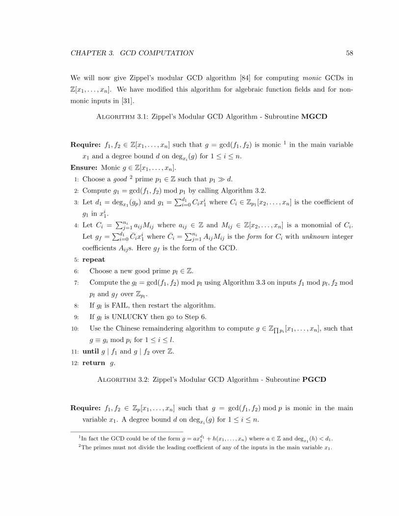
CHAPTER 3. GCD COMPUTATION 58
We will now give Zippel’s modular GCD algorithm [84] for computing monic GCDs in
Z[x1, . . . , xn]. We have modified this algorithm for algebraic function fields and for non-
monic inputs in [31].
Algorithm 3.1: Zippel’s Modular GCD Algorithm - Subroutine MGCD
Require: f1, f2 ∈ Z[x1, . . . , xn] such that g = gcd(f1, f2) is monic 1 in the main variable
x1 and a degree bound d on degxi(g) for 1 ≤ i ≤ n.
Ensure: Monic g ∈ Z[x1, . . . , xn].
1: Choose a good 2 prime p1 ∈ Z such that p1 d.
2: Compute g1 = gcd(f1, f2) mod p1 by calling Algorithm 3.2.
3: Let d1 = degx1(gp) and g1 =∑d1
i=0Cixi1 where Ci ∈ Zp1 [x2, . . . , xn] is the coefficient of
g1 in xi1.
4: Let Ci =∑ni
j=1 aijMij where aij ∈ Z and Mij ∈ Z[x2, . . . , xn] is a monomial of Ci.
Let gf =∑d1
i=0 Cixi1 where Ci =
∑nij=1AijMij is the form for Ci with unknown integer
coefficients Aijs. Here gf is the form of the GCD.
5: repeat
6: Choose a new good prime pl ∈ Z.
7: Compute the gl = gcd(f1, f2) mod pl using Algorithm 3.3 on inputs f1 mod pl, f2 mod
pl and gf over Zpl .8: If gl is FAIL, then restart the algorithm.
9: If gl is UNLUCKY then go to Step 6.
10: Use the Chinese remaindering algorithm to compute g ∈ Z∏pi [x1, . . . , xn], such that
g ≡ gi mod pi for 1 ≤ i ≤ l.11: until g | f1 and g | f2 over Z.
12: return g.
Algorithm 3.2: Zippel’s Modular GCD Algorithm - Subroutine PGCD
Require: f1, f2 ∈ Zp[x1, . . . , xn] such that g = gcd(f1, f2) mod p is monic in the main
variable x1. A degree bound d on degxi(g) for 1 ≤ i ≤ n.
1In fact the GCD could be of the form g = axd11 + h(x1, . . . , xn) where a ∈ Z and degx1(h) < d1.
2The primes must not divide the leading coefficient of any of the inputs in the main variable x1.

CHAPTER 3. GCD COMPUTATION 59
Ensure: Monic g ∈ Zp[x1, . . . , xn].
1: If n = 1 return the output of the Euclidean algorithm on inputs f1, f2 ∈ Zp[x1] .
2: Choose a good 3 evaluation point α1 ∈ Zp at random. Let a = f1(x1, . . . , xn−1, xn =
α1) mod p and b = f2(x1, . . . , xn−1, xn = α1) mod p. We have a, b ∈ Zp[x1, . . . , xn−1].
3: Apply Algorithm 3.2 recursively to compute g1 = gcd(a, b) mod p.
4: Let gf be the form of the GCD obtained from g1.
5: for i from 2 to d+ 1 do
6: Choose a good evaluation point αi ∈ Zp at random. Let a = f1(x1, . . . , xn−1, xn =
αi) mod p and b = f2(x1, . . . , xn−1, xn = αi) mod p.
7: Let gi be the output of Algorithm 3.3 on a, b ∈ Zp[x1, . . . , xn−1] and gf over Zp.8: If gi is FAIL then restart the algorithm.
9: If gi is UNLUCKY then go to Step 6.
10: end for
11: Use Newton’s interpolation algorithm (dense) to interpolate xn in g such that g ≡gi mod 〈xn − αi〉 for 1 ≤ i ≤ d+ 1 and degxi(g) ≤ d.
12: If g | f1 mod p and g | f2 mod p then return g otherwise restart the algorithm.
Algorithm 3.3: Zippel’s Sparse Interpolation Algorithm
Require: f1, f2 ∈ R[x1, . . . , xn] such that g = gcd(f1, f2) is monic in the main variable x1.
R here is the coefficient ring (either Z or Zp for some prime p). And gf , the form of the
GCD g which is of degree d1 in x1.
Ensure: Either fail (UNLUCKY or FAIL) or the monic GCD g ∈ R[x1, . . . , xn].
1: Let gf =∑d1
i=0 Cixi1 where Ci =
∑nij=1AijMij is the form for Ci, the coefficient of g in
xi1. Here the coefficient Aij ∈ R is unknown and Mij does not have x1.
2: Let N = max(n0, . . . , nd1) + 1 4 where ni is the number of non-zero terms in Ci.
3: Choose N random evaluation points βk = (α1, . . . , αn−1) ∈ Rn−1 (1 ≤ k ≤ N).
4: Let ak = f1(x1, βk) and bk = f2(x1, βk). We have ak, bk ∈ R[x1]. Use the Euclidean
algorithm to compute gk = gcd(ak, bk) ∈ R[x1] for 1 ≤ k ≤ N s.t. gk is monic.
5: If for some 1 ≤ k ≤ N , degx1(gk) < d1 then return FAIL. Recall that d1 = degx1(gf ).6: If for some 1 ≤ k ≤ N , degx1(gk) > d1 then choose a new evaluation point βk and
3The evaluation point α is good if lcx1(f1)(α) 6= 0 and lcx1(f2)(α) 6= 0.4The one extra evaluation point is to possibly detect any error in the form gf .

CHAPTER 3. GCD COMPUTATION 60
compute gk = gcd(ak, bk) ∈ R[x1]. Repeat this until degx1(gk) = d1 for 1 ≤ k ≤ N .
7: For 0 ≤ i ≤ d1, let Si be a linear system obtained by equating∑ni
j=1mkijAij to cki where
for 1 ≤ k ≤ N , cki is the coefficient of gk in xi1 and mkij = Mij(βk) ∈ R.
8: Solve the linear system of equations Si for 1 ≤ i ≤ d1. If Si is under-determined then
return UNLUCKY. If Si is inconsistent, then return FAIL. If the system is determined
and consistent, we have the values for the unknown Aijs. Substitute these values in gf
to obtain g ∈ R[x1, . . . , xn].
9: return g.
Zippel’s sparse interpolation assumed that if an image of a polynomial obtained from
a random evaluation point is zero, then the polynomial itself is zero with high probability.
Schwartz (Lemma 1.7) states that for α1, . . . , αn ∈ Zp, we would have f(α1, . . . , αn) = 0 for
non-zero f with probability at most dp where d = deg(f). In Algorithm 3.2, let α1 be the first
evaluation point. Let g = gcd(f1, f2) ∈ (Zp[xn])[x1, . . . , xn−1] and g =∑T
i=1CiMi where
Ci ∈ Zp[xn] and Mi is a monomial in x1, . . . , xn−1. The assumption in Zippel’s algorithm is
that if Ci(α1) ≡ 0 mod p then Ci ≡ 0 mod p with high probability 5.
One of the bottlenecks of Zippel’s modular GCD algorithm is the trial divisions which
are done to ensure that the GCD computed is correct (Step 11 of Algorithm 3.1 and Step 12
of Algorithm 3.2). These trial divisions are often expensive, especially if the GCD is dense.
The SparseModGcd Algorithm
Our main goal in this chapter is improving the SparseModGcd algorithm we presented
in [30, 31]. Let F = Q(t1, . . . , tk). For i, 1 ≤ i ≤ r, let mi(z1, . . . , zi) ∈ F [z1, . . . , zi] be monic
and irreducible over F [z1, . . . , zi−1]/ 〈m1, . . . ,mi−1〉. Let L = F [z1, . . . , zr] / 〈m1, . . . ,mr〉.L is an algebraic function field in k parameters t1, . . . , tk. Suppose f1 and f2 are non-zero
polynomials in L[x1, . . . , xn]. The SparseModGcd algorithm will compute g or an associate
(scalar multiple) of g. The algorithm is modular and uses Zippel’s sparse interpolation
algorithm. We also use rational function reconstruction to recover the coefficients of the
GCD, when interpolating a parameter or a variable. Before getting into the details of the
improvements we need to give some definitions.
Definition 3.1. Let D = Z[t1, . . . , tk]. A non-zero polynomial in D[z1, . . . , zr, x] is said to
be primitive with respect to (z1, . . . , zr, x) if the GCD of its coefficients in D is 1. Let f be
5According to Lemma 1.7, if Ci(α) ≡ 0 mod p than Prob(Ci 6= 0 mod p) ≤ deg(Ci(x2,...,xn))p

CHAPTER 3. GCD COMPUTATION 61
non-zero in L[x] where L is the algebraic function field previously defined. The denominator
of f is the polynomial den(f) ∈ D of least total degree in (t1, . . . , tk) and with smallest
integer content such that den(f)f is in D[z1, . . . , zr, x]. The primitive associate f of f is the
associate of den(f)f which is primitive in D[z1, . . . , zr, x] and has positive leading coefficient
in a term ordering.
The following is an example from [31].
Example 3.2. Let f = 3tx2 + 6tx/(t2 − 1) + 30tz/(1− t) where m1(z) = z2 − t. Here
f ∈ L[x] where L = Q(t)[z]/⟨z2 − t
⟩is an algebraic function field in one parameter t. We
have den(f) = t2 − 1 and f = den(f)f/(3t) = (t2 − 1)x+ 2x− 10z(t+ 1).
Definition 3.3 (See [9]). Recall that for a polynomial f = anxn + · · · + a1x + a0 where
f ∈ F[x] the content of f in x is
contx(f) = gcd(a0, a1, . . . , an) ∈ F.
A prime p, is said to introduce an unlucky content if for two input polynomials f1, f2 ∈F[x1, . . . , xn] with GCD g = gcd(f1, f2), contx1(g) = 1 but contx1(g mod p) 6= 1. Similarly
an evaluation point xi = αj ∈ F is said to introduce an unlucky content if contx1(g) = 1
but contx1(g(xj = αj)) 6= 1.
Here is an example of an unlucky content from [31].
Example 3.4. Suppose g = (12s+t)x+(s+12t)z. We have contx(g) = gcd(12s+t, s+12t) =
1. But for p = 11 we obtain contx(g mod p) = s + t. Hence p = 11 introduces an unlucky
content and, for any prime p (other than 2 and 3), the evaluation points t = 0 and s = 0
introduce unlucky contents.
Suppose during sparse interpolation we choose our assumed form, gf , based on an image
which is computed modulo a prime (or evaluation point) which introduced an unlucky
content, e.g. p1 = 11 in our example. Then the assumed form gf will have different terms
in x, z1, . . . , zr, t1, . . . , tk than in g. This will with high probability result in an inconsistent
linear system during sparse interpolation.
Suppose instead that our assumed form gf is correct but it is a subsequent prime or
evaluation point that introduces an unlucky content. This may lead to an under-determined
linear system.

CHAPTER 3. GCD COMPUTATION 62
Example 3.5. Consider f1 = f2 = zx + t + 1 where m(z) = z2 − t − 14. Here g =
x+ (t+ 1)/(t+ 14)z and hence g = (t+ 14)x+ (t+ 1)z thus p = 13 introduces an unlucky
content t + 1. Suppose our first prime is p1 6= 13 and we obtain the correct assumed form
gf = (At + B)x + (Ct + D)z. Suppose our second prime is p2 = 13 and we perform a
sparse interpolation in t using t = 1, 2, 3, . . . . Since gf is not monic in x we will equate
gf (t) = mtg(t) and solve for A,B,C,D,m1,m2, . . . with m1 = 1. For t = 1, 2, 3 we obtain
the following equations modulo 13.
(A+B)x+ (C +D)z = m1(x+ z),
(2A+B)x+ (2C +D)z = m2(x+ z),
(3A+B)x+ (3C +D)z = m3(x+ z).
Equating coefficients of xizj we obtain the following linear system: A+B = m1, 2A+B =
m2, 3A + B = m3, C + D = 1, 2C + D = 1, 3C + D = 1. The reader may verify that this
system, with m1 = 1, is not determined, and also, adding further equations, for example,
from t = 4, does not make the system determined.
If the system of linear equations is not determined (with one more image than necessary),
SparseModGcd will assume that the current prime or one of the evaluations has caused an
unlucky content. In this case the algorithm restarts with a new prime (Similar to Step 8 of
Algorithm 3.3).
The main bottleneck of the SparseModGcd algorithm presented in [31] on sparse input
polynomials is computing the univariate GCDs of polynomials over an algebraic number ring
modulo a prime p. In Section 3.1 we will discuss how we can improve this by implementing
an in-place GCD algorithm. In Section 3.2 we will prove that the probability of algorithm
MQRR making an error is low. We will also give the probability that Zippel’s sparse
interpolation will succeed, given a wrong form (due to the error in the output of MQRR).
Using these we prove that we can eliminate the trial divisions in positive characteristic. In
Section 3.3 we will show that the previous solution given for normalization problem in [9]
has an error. We will give a new solution for this problem and prove that this solution
works.

CHAPTER 3. GCD COMPUTATION 63
3.1 Univariate GCDs over Algebraic Number Fields
In 2002, van Hoeij and Monagan in [70] presented an algorithm for computing the monic
GCD g(x) of two polynomials f1(x) and f2(x) in L[x] where L = Q(α1, α2, . . . , αk) is an
algebraic number field. The algorithm is a modular GCD algorithm. It computes the GCD
of f1 and f2 modulo a sequence of primes p1, p2, . . . , pl using the monic Euclidean algorithm
in Lp[x] (Lp = L mod p) and it reconstructs the rational numbers in g(x) using Chinese
remaindering and rational number reconstruction. The algorithm is a generalization of
earlier work of Langymyr and MaCallum [48], and Encarnacion [12] to treat the case where
L has multiple extensions (k > 1). It can be generalized to multivariate polynomials in
L[x1, x2, . . . , xn] using evaluation and interpolation (see [71, 31]).
Monagan implemented the algorithm in Maple in 2001 and in Magma in 2003 using
the recursive dense polynomial representation to represent elements of L, Lp, L[x1, . . . , xn]
and Lp[x1, . . . , xn]. This representation is generally more efficient than the distributed and
recursive sparse representations for sparse polynomials. See for example the comparison
by Fateman in [14]. And since efficiency in the recursive dense representation improves
for dense polynomials, and elements of L are often dense, it should be a good choice for
implementing arithmetic in L and also Lp.
However, we have observed that arithmetic in Lp is very slow when α1 has low degree.
Since this case often occurs in practical applications, and since over 90% of a GCD compu-
tation in L[x] is typically spent in the Euclidean algorithm in Lp[x], we sought to improve
the efficiency of the arithmetic in Lp. One reason why this happens is because the cost
of storage management, allocating small arrays for storing intermediate polynomials of low
degree can be much higher than the cost of the actual arithmetic being done in Zp.We explain why this is the case with an example.
Example 3.6. Let L = Q(α1, α2) where α1 =√
2 and α2 = 3√
1/5 + α1. L is an algebraic
number field of degree d = 6 over Q. We represent elements of L as polynomials in Q[u][v]
and we do arithmetic in L modulo the ideal I = 〈m1(u),m2(v, u)〉 where m1(u) = u2 − 2
and m2(v, u) = v3 − u− 1/5 are the minimal polynomials for α1 and, respectively, α2.
To implement the modular GCD algorithm one uses machine primes, that is, the largest
available primes that fit in the word of the computer so that arithmetic in Zp can be
done by the computer’s hardware. After choosing the next machine prime p, we build
the ring Lp[x] where Lp = L mod p, iteratively, as follows; first we build the residue ring

CHAPTER 3. GCD COMPUTATION 64
Lu = Zp[u]/〈u2− 2 mod p〉. We use a dense array of machine integers to represent elements
of Lu. Then we build Lv = Lu[v]/〈v3 − u − 1/5 mod p〉 and finally the polynomial ring
Lp[x]. In the recursive dense representation we represent elements of Lv as dense arrays of
pointers to elements of Lu. So a general element of Lv, which looks like
(a1u+ b1)v2 + (a2u+ b2)v + (a3u+ b3),
would be stored as follows where the degree of each element is explicitly stored.
1 b3 a3 1 b2 a2 1 b1 a1 ∈ Lu
2
+
SSSw
∈ Lv
When the monic Euclidean algorithm is executed in Lp[x], it will do many multiplications
and additions of elements in Lv, each of which will do many in Lu. This results in many calls
to the storage manager to allocate small arrays for intermediate and final results in Lu and
Lv and rapidly produces a lot of small pieces of garbage. Consider one such multiplication
in Lu
(au+ b)(cu+ d) mod u2 − 2.
The algorithms compute the product P = acu2 + (ad + bc)u + bd and then divide P by
u2 − 2 to get the remainder R = (ad + bc)u + (bd + 2ac). They allocate arrays to store
the polynomials P and R. We have observed that, even though the storage manager is not
inefficient, the cost of these storage allocations and the other overhead for arithmetic in
Zp[u]/〈u2−2〉 overwhelms the cost of the actual integer arithmetic in Zp needed to compute
(ad+ bc) mod p and (bd+ 2ac) mod p.
Our main contribution is a library of in-place 6 algorithms for arithmetic in Lp and Lp[x]
where Lp has one or more extensions. The main idea is to eliminate all calls to the storage
manager by pre-allocating one large piece of working storage, and re-using parts of it in a
computation. In Section 3.1.1 we describe the recursive dense polynomial representation for
6In-place here means the total amount of storage required is pre-computed so that only one call to thestorage allocator is necessary. This storage is used many times for intermediate results. The term in-placeis also used for algorithms which overwrite their input buffer with the output (See e.g. [25]).

CHAPTER 3. GCD COMPUTATION 65
elements of Lp[x]. In Section 3.1.2 we present algorithms for multiplication and inversion in
Lp and multiplication, division with remainder and GCD in Lp[x] which are given one array
of storage in which to write the output and one additional array W of working storage for
intermediate results. In Section 3.1.3 we give formula for determining the size of W needed
for each algorithm. In each case the amount of working storage is linear in d the degree of
L. We have implemented our algorithms in the C language in a library which includes also
algorithms for addition, subtraction, and other utility routines. In Section 3.1.4 we present
benchmarks demonstrating its efficiency by comparing our algorithms with the Magma ([4])
computer algebra system and we explain how to avoid most of the integer divisions by p
when doing arithmetic in Zp because this also significantly affects overall performance.
3.1.1 Polynomial Representation
Let Q(α1, α2, . . . , αr) be our number field L. We build L as follows. For 1 ≤ i ≤ r,
let mi(z1, . . . , zi) ∈ Q[z1, . . . , zi] be the minimal polynomial for αi, monic and irreducible
over Q[z1, . . . , zi−1]/ 〈m1, . . . ,mi−1〉. Let di = degzi(mi). We assume di ≥ 2. Let L =
Q[z1, . . . , zr]/ 〈m1, . . . ,mr〉. So L is an algebraic number field of degree d =∏di over
Q. For a prime p for which the rational coefficients of mi exist modulo p, let Ri =
Zp[z1, . . . , zi]/ 〈m1, . . . , mi〉 where mi = mi mod p and let R = Rr = L mod p. We use
the following recursive dense representation for elements of R and polynomials in R[x] for
our algorithms. We view an element of Ri+1 as a polynomial with degree at most di+1 − 1
with coefficients in Ri.
To represent a non-zero element β1 = a0 + a1z1 + · · ·+ ad1−1zd1−11 ∈ R1 we use an array
A1 of size S1 = d1 + 1 indexed from 0 to d1, of integers (modulo p) to store β1. We store
A1[0] = degz1(α1) and, for 0 ≤ i < d1 : A1[i+ 1] = ai. Note that if degz1(α1) = d < d1 − 1
then for d+ 1 < j ≤ d1, A1[j] = 0. To represent the zero element of R1 we use A[0] = −1.
Now suppose we want to represent an element β2 = b0+b1z2+· · ·+bd2−1zd2−12 ∈ R2 where
bi ∈ R1 using an array A2 of size S2 = d2S1 +1 = d2(d1 +1)+1. We store A2[0] = degz2(β2)
and for 0 ≤ i < d2
A2[i(d1 + 1) + 1 . . . (i+ 1)(d1 + 1)] = Bi[0 . . . d1],
where Bi is the array which represents bi ∈ R1. Again if β2 = 0 we store A2[0] = −1.
Similarly, we recursively represent βr = c0 + c1zr + · · · + cdr−1zdr−1r ∈ Rr based on the
representation of ci ∈ Rr−1. Let Sr = drSr−1 + 1 and suppose Ar is an array of size Sr such

CHAPTER 3. GCD COMPUTATION 66
that Ar[0] = degzr(βr) and for 0 ≤ i < dr
Ar[i(dr−1) + 1 . . . (i+ 1)(dr−1 + 1)] = Ci[0 . . . Sr−1 − 1].
Note, we store the degrees of the elements of Ri in Ai[0] simply to avoid re-computing them.
We haver∏i=1
di < Sr <r∏i=1
(di + 1), Sr ∈ O(r∏i=1
di).
Now suppose we use the array C to represent a polynomial f ∈ Ri[x] of degree dx in the
same way. Each coefficient of f in x is an element of Ri which needs an array of size Si,
hence C must be of size
P (dx, Ri) = (dx + 1)Si + 1.
Example 3.7. Let r = 2 and p = 17. Let m1 = z31 +3, m2 = z2
2 +5z1z2 +4z2 +7z21 +3z1 +6,
and f = 3 + 4z1 + (5 + 6z1)z2 + (7 + 8z1 + 9z21 + (10z1 + 11z2
1)z2)x+ 12x2.
The representation for f is
C = 2 1 1 3 4 0 1 5 6 0︸ ︷︷ ︸3+4z1+(5+6z1)z2
1 2 7 8 9 2 0 10 11︸ ︷︷ ︸10z1+11z21
0 0 12 0 0 −1 0 0 0
Here dx = 2, d1 = 3, d2 = 2, S1 = d1 + 1 = 4, S2 = d2S1 + 1 = 9 and the size of the array A
is P (dx, R2) = (dx + 1)S2 + 1 = 28.
We also need to represent the minimal polynomial mi. Let mi = a0 + a1zi + . . . adizdii
where aj ∈ Ri−1. We need an array of size Si−1 to represent aj so to represent mi in the same
way we described above, we need an array of size Si = 1+(di+1)Si−1 = diSi−1 +1+Si−1 =
Si + Si−1. We define S0 = 1.
We represent minimal polynomials m1, . . . , mr as an array E, of size∑r
i=1 Si =∑ri=1 (Si + Si−1) = 1 + Sr + 2
∑r−1i=1 Si such that E[Mi . . .Mi+1 − 1] represents mr−i where
M0 = 0 and Mi =∑r
i=r−i+1 Si. The minimal polynomials in Example 3.7 will be rep-
resented in the following figure where E[0 . . . 12] represents m2 and E[13 . . . 17] represents
m1.
E = 2 2 6 3 7 1 4 5 0 0 1 0 0︸ ︷︷ ︸m2
3 3 0 0 1︸ ︷︷ ︸m1

CHAPTER 3. GCD COMPUTATION 67
3.1.2 In-place Algorithms
In this section we design efficient in-place algorithms for multiplication, division and GCD
computation of two univariate polynomials over R. We will also give an in-place algorithm
for computing the inverse of an element α ∈ R, if it exists. This is needed for making
a polynomial monic for the monic Euclidean algorithm in R[x]. We assume the following
utility operations are implemented.
• IP ADD(N,A,B) and IP SUB(N,A,B) are used for in-place addition and subtraction of two
polynomials a, b ∈ RN [x] represented in arrays A and B.
• IP MUL NO EXT is used for multiplication of two polynomials over Zp. A description of this
algorithm is given in Section 3.1.4.
• IP REM NO EXT is used for computing the quotient and the remainder of dividing two
polynomials over Zp.
• IP INV NO EXT is used for computing the inverse of an element in Zp[z] modulo a minimal
polynomial m ∈ Zp[z].
• IP GCD NO EXT is used for computing the GCD of two univariate polynomials over Zp (the
Euclidean algorithm, See [58]).
In-place Multiplication
Suppose we have a, b ∈ R[x] where R = Rr−1[zr]/〈mr(zr)〉. Let a =∑da
i=0 aixi and b =∑db
i=0 bixi where da = degx(a) and db = degx(b) and Let c = a × b =
∑dci=0 cix
i where
dc = degx(c) = da + db. To reduce the number of divisions by mr(zr) when multiplying
a× b, we use the Cauchy product rule to compute ck as suggested in [58], that is,
ck =
min(k,da)∑i=max(0,k−db)
ai × bk−i
mod mr(zr).
Thus the number of multiplications in Rr−1[zr] (in line 11) is (da + 1) × (db + 1) and the
number of divisions in Rr−1[zr] (in line 15) is da + db + 1.
The number of iterations in the loop in line 10 is K = min(k, da)−max(0, k − db) + 1. We
have 0 ≤ k ≤ dc = da + db thus
1 ≤ K ≤ min(da, db) + 1.
Here instead of doing K divisions in Rr−1[zr], we do only one. This saves about half the
work.

CHAPTER 3. GCD COMPUTATION 68
Algorithm 3.4: Algorithm IP MUL: In-place Multiplication
Require: • N the number of field extensions.
• Arrays A[0 . . . a] and B[0 . . . b] representing univariate polynomials a, b ∈ RN [x]
(RN = Zp[z1, . . . , zN ]/ 〈m1, . . . , mN 〉). Note that a = P (da, RN ) − 1 and b =
P (db, RN )− 1 where da = degx(a) and db = degx(b).
• Array C[0 . . . c]: Space needed for storing c = a × b =∑dc
i=0 cixi where c =
P (degx(a) + degx(b), RN )− 1.
• E[0 . . . eN ] : representing the set of minimal polynomials where eN = SN +
2∑N−1
i=1 Si.
• W [0 . . . wN ] : the working storage for the intermediate operations.
Ensure: For 0 ≤ k ≤ dc, ck will be computed and stored in C[kSN + 1 . . . (k + 1)SN ].
1: Set da := A[0] and db := B[0].
2: if da = −1 or db = −1 then Set C[0] := −1 and return.
3: if N = 0 then Call IP MUL NO EXT on inputs A, B and C and return.
4: Let M = E[0 . . . SN − 1] and E′ = E[SN . . . eN ] M points to mN in E[0 . . . eN ].5: Let T1 = W [0 . . . t − 1] and T2 = W [t . . . 2t − 1] and W ′ = W [2t . . . wN ] where t =
P (2dN − 2, RN−1) and dN = M [0] = degzN (mN ).
6: Set dc := da + db and sc := 1.
7: for k from 0 to dc do
8: Set sa := 1 + iSN and sb := 1 + (k − i)SN .
9: Set T1[0] := −1 T1 = 0.10: for i from max(0, k − db) to min(k, da) do
11: Call IP MUL(N − 1, A[sa . . . a], B[sb . . . b], T2, E′,W ′).
12: Call IP ADD(N − 1, T1, T2) T1 := T1 + T213: Set sa := sa + SN and sb := sb − SN .
14: end for
15: Call IP REM(N − 1, T1,M,E′,W ′). Reduce T1 modulo M = mN.16: Copy T1[0 . . . SN − 1] into C[sc . . . sc+ SN − 1].
17: Set sc := sc + SN .
18: end for

CHAPTER 3. GCD COMPUTATION 69
19: Determine degx(a× b): There might be zero-divisors.20: Set i := dc and sc := sc − SN .
21: while i ≥ 0 and C[sc] = −1 do Set i := i− 1 and sc := sc − SN .
22: Set C[0] := i.
The temporary variables T1 and T2 must be big enough to store the product of two
coefficients in a, b ∈ RN [x]. Coefficients of a and b are in RN−1[zN ] with degree (in zN )
at most dN − 1. Hence these temporaries must be of size P (dN − 1 + dN − 1, RN−1) =
P (2dN − 2, RN−1).
In-place Division
The following algorithm divides a polynomial a ∈ RN [x] by a monic polynomial b ∈ RN [x].
The remainder and the quotient of a divided by b will be stored in the array representing
a hence a is destroyed by the algorithm. The division algorithm is organized differently
from the normal long division algorithm which does db × (da − db + 1) multiplications and
divisions in RN−1[zr]. The total number of divisions by M in RN−1[zr] in line 16 is reduced
to da + 1 (see line 8).
The number of iterations in the loop in line 11 is K = min(Dr, k)−max(0, k−Dq) + 1. We
have 0 ≤ k ≤ da thus
1 ≤ K ≤ min(Dr, Dq) + 1 = min(db, da − db + 1).
Here instead of doing K divisions in RN−1[zr], we do only one. This saves about half the
work.
Algorithm 3.5: Algorithm IP REM: In-place Remainder
Require: • N the number of field extensions.
• Arrays A[0 . . . a] and B[0 . . . b] representing univariate polynomials a, b 6= 0 ∈RN [x] (RN = Zp[z1, . . . , zN ]/ 〈m1, . . . , mN 〉) where da = degx(a) ≥ da = degx(b).
Note b must be monic and a = P (da, RN )− 1 and b = P (db, RN )− 1.
• E[0 . . . eN ] : representing the set of minimal polynomials where eN = SN +
2∑N−1
i=1 Si.

CHAPTER 3. GCD COMPUTATION 70
• W [0 . . . wN ] : the working storage for the intermediate operations.
Ensure: The remainder R of a divided by b will be stored inA[0 . . . r] where r = P (D,RN )−1 and D = degx(R) ≤ db − 1. Also let Q represent the quotient Q of a divided by b.
Q[1 . . . q] will be stored in A[1 + dbSN . . . a] where q = P (da − db, RN )− 1.
1: Set da := A[0] and db := B[0].
2: if da < db then return.
3: if N = 0 then Call IP REM NO EXT on inputs A and B and return.
4: Set Dq := da − db and Dr := db − 1.
5: Let M = E[0 . . . SN − 1] and E′ = E[SN . . . eN ] M points to mN in E[0 . . . eN ].6: Let T1 = W [0 . . . t − 1] and T2 = W [t . . . 2t − 1] and W ′ = W [2t . . . wN ] where t =
P (2dN − 2, RN−1) and dN = M [0] = degzN (mN ).
7: Set sc := 1 + daSN
8: for k = da to 0 by −1 do
9: Copy A[sc . . . sc+ SN − 1] into T1[0 . . . SN − 1].
10: Set i := max(0, k −Dq), sb := 1 + iSN and sa := 1 + (k − i+ db)SN .
11: while i ≤ min(Dr, k) do
12: Call IP MUL(N − 1, A[sa . . . a], B[sb . . . b], T2, E′,W ′).
13: Call IP SUB(N − 1, T1, T2) T1 := T1 − T2.14: Set sb := sb + SN and sa := sa − SN .
15: end while
16: Call IP REM(N − 1, T1, M , E′,W ′) Reduce T1 modulo M = mN.17: Copy T1[0 . . . SN − 1] into A[sc . . . sc + SN − 1].
18: Set sc := sc − SN .
19: end for
20: Set i := Dr and sc := 1 +DrSN .
21: while i ≥ 0 and A[sc] = −1 do Set i := i− 1 and sc := sc − SN .
22: Set A[0] := i.
Let arrays A and B represent polynomials a and b respectively. Let da = degx(a) and
db = degx(b). Array A has enough space to store da + 1 coefficients in RN plus one unit
of storage to store da. Hence the total storage is (da + 1)SN + 1. The remainder R is of
degree at most db − 1 in x, i.e. R needs storage for db coefficients in RN and one unit for
the degree. Similarly the quotient Q is of degree da− db, hence needs storage for da− db + 1
coefficients and one unit for the degree. Thus the remainder and the quotient together need

CHAPTER 3. GCD COMPUTATION 71
dbSN +1+(da−db+1)SN +1 = (da+1)SN +2. This means we are one unit of storage short
if we want to store both R and Q in A. This is because this time we are storing two degrees
for Q and R. Our solution is that we will not store the degree of Q. Any algorithm that
calls IP REM and needs both the quotient and the remainder must use degx(a) − degx(b)
for the degree of Q.
After applying this algorithm the remainder R will be stored in A[0 . . . dbSN ] and the
quotient Q minus the degree will be stored in A[dbSN . . . (da + 1)SN ]. Similar to IP MUL,
the remainder operation in line 16 has been moved to outside of the main loop to let the
values accumulate in T1.
Computing (In-place) the inverse of an element in RN
In this algorithm we assume the following in-place function:
• IP SCAL MUL(N,A,C,E,W ): This is used for multiplying a polynomial a ∈ RN [x]
(represented by array A) by a scalar c ∈ RN (represented by array C). The algorithm
will multiply every coefficient of a in x by c and reduce the result modulo the minimal
polynomials. It can easily be implemented using IP MUL and IP REM.
The algorithm computes the inverse of an element a in RN . If the element is not
invertible, then the Euclidean algorithm will compute a proper divisor of some minimal
polynomial mi(zi), a zero-divisor in Ri. The algorithm will store that zero-divisor in the
space provided for the inverse and return the index i of the minimal polynomial which is
reducible and has caused the zero-divisor.
Algorithm 3.6: Algorithm IP INV: In-place inverse of an element in RN
Require: • N the number of field extensions.
• Array A[0 . . . a] representing the univariate polynomial a ∈ RN . Note that N ≥ 1
and a = SN − 1.
• Array I[0 . . . i]: Space needed for storing the inverse a−1 ∈ RN . Note that i =
SN − 1.
• E[0 . . . eN ] : representing the set of minimal polynomials. Note that eN = SN +
2∑N−1
i=1 Si.

CHAPTER 3. GCD COMPUTATION 72
• W [0 . . . wN ] : the working storage for the intermediate operations.
Ensure: The inverse of a (or a zero-divisor, if there exists one) will be computed and stored
in I. If there is a zero-divisor, the algorithm will return the index k where mk is the
reducible minimal polynomial, otherwise it will return 0.
1: Let M = E[0 . . . SN − 1] and E′ = E[SN . . . eN ] M = mN.2: if N = 1 then Call IP INV NO EXT on inputs A, I, E,M and W and return.
3: if A[i] = 0, for all 0 ≤ i < N and A[N ] = 1 Test if a = 1 then
4: Copy A into I and return 0.
5: end if
6: Let r1 = W [0 . . . t−1], r2 = W [t . . . 2t−1], s1 = I, s2 = W [2t . . . 3t−1], T = W [3t . . . 4t−1], T ′ = W [4t . . . 4t+ t′ − 1] and W ′ = W [4t+ t′ . . . wN ] where t = P (dN , RN−1)− 1 =
SN − 1, t′ = P (2dN − 2, RN−1) and dN = M [0] = degzN (mN ).
7: Copy A and M into r1 and r2 respectively.
8: Set s2[0] := −1 s2 represents 0.9: Let Z ∈ Z := IP INV(N − 1, A[DaSN−1 + 1 . . . a], T, E′,W ′) where Da = A[0] =
degzN (a). A[DaSN−1 + 1 . . . a] represents l = lczN (a) and T represents l−1.10: if Z > 0 then Copy T into I and return Z.
11: Copy T into s1.
12: Call IP SCAL MUL(N, r1, T, E′,W ′) r1 is made monic.
13: while r2[0] 6= −1 do
14: Set Z = IP INV(N − 1, r2[Dr2SN−1 + 1 . . . a], T, E′,W ′) where Dr2 = degzN (r2).
15: if Z > 0 then Copy T into I and return Z.
16: Call IP SCAL MUL(N, r2, T, E′,W ′) r2 is made monic.
17: Call IP SCAL MUL(N, s2, T, E′,W ′).
18: Set Dq := max(−1, r1[0]− r2[0]).
19: Call IP REM(N, r1, r2, E′,W ′).
20: Swap the arrays r1 and r2. Interchange only the pointers.21: Set t1 := r2[r1[0]SN−1] and set r2[r1[0]SN−1] := Dq.
22: Call IP MUL(N − 1, q, s2, T′, E′,W ′) where q = r2[r1[0]SN−1 . . . a].
23: Call IP REM(N −1, T ′,M,E′,W ′) and then IP SUB(N −1, s1, T′). s1 := s1− qs2
24: Set r2[r1[0]SN−1] := t1.
25: Swap the arrays s1 and s2. Interchange only the pointers.26: end while

CHAPTER 3. GCD COMPUTATION 73
27: if r1[i] = 0 for all 0 ≤ i < N and r1[N ] = 1 then
28: Copy s1 into I r1 = 1 and s1 is the inverse and return 0.
29: else
30: Copy r1 into I r1 6= 1 is the zero-divisor and return N − 1 mN−1 is reducible.31: end if
As discussed in Section 3.1.2, IP REM will not store the degree of the quotient of a
divided by b hence in line 21 we explicitly compute and set the degree of the quotient before
using it to compute s1 := s1− qs2 in lines 22 and 23. Here r2[r1[0]SN−1 . . . a] is the quotient
of dividing r1 by r2 in line 19.
In-place GCD Computation
In the following algorithm we compute the GCD of a, b ∈ RN [x] using the monic Euclidean
algorithm. This is the main subroutine used to compute univariate images of a GCD in L[x]
for the algorithm in [70] and images of a multivariate GCD over an algebraic function field for
our algorithm in [31]. Note, since mi(zi) may be reducible modulo p, RN is is not necessarily
a field, and therefore, the monic Euclidean algorithm may encounter a zero-divisor in RN
when calling subroutine IP INV.
Algorithm 3.7: Algorithm IP GCD: In-place GCD Computation
Require: • N the number of field extensions.
• Arrays A[0 . . . a] and B[0 . . . b] representing univariate polynomials a, b 6= 0 ∈RN [x] (RN = Zp[z1, . . . , zN ]/ 〈m1, . . . , mN 〉) where da = degx(a) ≥ da = degx(b)
and A,B 6= 0. Note that b is monic and a = P (da, RN )−1 and b = P (db, RN )−1.
• E[0 . . . eN ] : representing the set of minimal polynomials where eN = SN +
2∑N−1
i=1 Si.
• W [0 . . . wN ] : the working storage for the intermediate operations.
Ensure: If there exist a zero-divisor, it will be stored in A and the index of the reducible
minimal polynomial will be returned. Otherwise the monic GCD g = gcd(a, b) will be
stored in A and 0 will be returned.
1: if N = 0 then CALL IP GCD NO EXT on inputs A and B and return 0.

CHAPTER 3. GCD COMPUTATION 74
2: Set da := A[0] and db := B[0].
3: Let r1 and r2 point to A and B respectively.
4: Let I = W [0 . . . t− 1] and W ′ = W [t . . . wN ] where t = SN − 1 = SN + SN−1 − 1.
5: Let Z be the output of IP INV(N, r1[1 + r1[0]SN . . . a], I, E,W ′).
6: if Z > 0 then Copy I into A and return Z.
7: Call IP SCAL MUL(N, r1, I, E,W′).
8: while r2[0] 6= −1 do
9: Let Z be the output of IP INV(N, r2[1 + r2[0]SN . . . b], I, E,W ′).
10: if Z > 0 then Copy I into A and return Z.
11: Call IP SCAL MUL(N, r2, I, E,W′).
12: Call IP REM(N, r1, r2, E,W′).
13: Swap r1 and r2 interchange pointers.14: end while
15: Copy r1 into A.
16: return 0.
Similar to the algorithm IP INV, if there exists a zero-divisor, i.e. the leading coefficient
of one of the polynomials in the polynomial remainder sequence is not invertible, in steps 6
and 10 the algorithm stores the zero-divisor in the space provided for a and returns Z the
index of the minimal polynomial which is reducible and has caused the zero-divisor.
3.1.3 Working Space
In this section we will determine recurrences for the exact amount of working storage wN
needed for each operation introduced in the previous section. Recall that di = degzi(mi) is
the degree of the ith minimal polynomial which we may assume is at least 2. Also Si is the
space needed to store an element in Ri and we have Si+1 = di+1Si + 1 and S1 = d1 + 1.
Lemma 3.8. SN > 2SN−1 for N > 1.
Proof. We have SN = dNSN−1 + 1 where dN = degzN (mN ). Since dN ≥ 2 we have SN ≥2SN−1 + 1⇒ SN > 2SN−1.
Lemma 3.9.∑N−1
i=1 Si < SN for N > 1.
Proof. (by induction on N). For N = 2 we have∑1
i=1 Si = S1 < S2. For N = k + 1 ≥ 2
we have∑k
i=1 Si = Sk +∑k−1
i=1 Si. By induction we have∑k−1
i=1 Si < Sk hence∑k
i=1 Si <

CHAPTER 3. GCD COMPUTATION 75
Sk + Sk = 2Sk. Using Lemma 3.8 we have 2Sk < Sk+1 hence∑k
i=1 Si < 2Sk < Sk+1 and
the proof is complete.
Corollary 3.10.∑N
i=1 Si < 2SN for N > 1.
Lemma 3.11. P (2dN − 2, RN−1) = 2SN − SN−1 − 1 for N > 1.
Proof. We have P (2dN−2, RN−1) = (2dN−1)SN−1+1 = 2dNSN−1−SN−1+1 = 2(dNSN−1+
1)− SN−1 − 1 = 2SN − SN−1 − 1.
Multiplication and Division Algorithms
Let M(N) be the amount of working storage needed to multiply a, b ∈ RN [x] using the
algorithm IP MUL. Similarly let Q(N) be the amount of working storage needed to divide
a by b using the algorithm IP REM. The working storage used in lines 5,11 and 15 of
algorithm IP MUL and lines 6,12 and 16 of algorithm IP REM is
M(N) = 2P (2dN − 2, RN−1) + max(M(N − 1), Q(N − 1)) and (3.1)
Q(N) = 2P (2dN − 2, RN−1) + max(M(N − 1), Q(N − 1)). (3.2)
Comparing equations (3.1) and (3.2) we see that M(N) = Q(N) for any N ≥ 1. Hence
M(N) = 2P (2dN − 2, RN−1) +M(N − 1). (3.3)
Simplifying (3.3) gives M(N) = 2SN − 2N + 2∑N
i=1 Si. Using Corollary 3.10 we have
Theorem 3.12. M(N) = Q(N) = 2SN − 2N + 2∑N
i=1 Si < 6SN .
Remark 3.13. When calling the algorithm IP MUL to compute c = a×b where a, b ∈ R[x],
we should use a working storage array W [0 . . . wn] such that wn ≥ M(N). Since M(N) <
6SN , the working storage must be big enough to store only six coefficients in Lp.
Let C(N) denote the working storage needed for the operation IP SCAL MUL. It is
easy to show that C(N) = M(N − 1) + P (2dN − 2, RN−1) < M(N).

CHAPTER 3. GCD COMPUTATION 76
Inversion
Let I(N) denote the amount of working storage needed to invert c ∈ RN . In lines 6, 9, 12,
14, 16, 17, 19 , 22 and 23 of algorithm IP INV we use the working storage. We have
I(N) = 4P (dN , RN−1) + P (2dN − 2, RN−1) + max(I(N − 1),M(N − 1), Q(N − 1)). (3.4)
But we have M(N − 1) = Q(N − 1), hence
I(N) = 4P (dN , RN−1) + P (2dN − 2, RN−1) + max(I(N − 1),M(N − 1)). (3.5)
Lemma 3.14. For N ≥ 1, we have M(N) < I(N).
Proof. The proof is by contradiction. Assume M(N) ≥ I(N). Using (3.5) we have I(N) =
4P (dN , RN−1) +P (2dN − 2, RN−1) + M(N − 1). On the other hand using (3.3) we have
M(N) = 2P (2dN − 2, RN−1) + M(N − 1). We assumed I(N) ≤ M(N) hence we have
4P (dN , RN−1) + P (2dN − 2, RN−1) + M(N − 1) ≤ 2P (2dN − 2, RN−1) + M(N − 1) thus
4P (dN , RN−1) + P (2dN − 2, RN−1) ≤ 2P (2dN − 2, RN−1) ⇒ 6SN + 3SN−1 − 1 ≤ 4SN −2SN−1 − 2 which is a contradiction. Thus I(N) > M(N).
Using Equation (3.4) and Lemma 3.14 we conclude that I(N) = 4P (dN , RN−1)+P (2dN−2, RN−1) + I(N − 1). Simplifying this yields:
Theorem 3.15. I(N) = 4∑N
i=1 P (di, Ri−1)+∑N
i=1 P (2di − 2, Ri−1) = 4∑N
i=1 (Si + Si−1)+∑Ni=1 (2Si − Si−1 − 1) = 6SN + 9
∑N−1i=1 Si −N.
Using Lemma 3.8 an upper bound for I(N) is I(N) < 6SN + 9SN = 15SN .
GCD Computation
Let G(N) denote the working storage needed to compute the GCD of a, b ∈ RN [x]. In
lines 4,5,7,9,11 and 12 of algorithm IP GCD we use the working storage. We have G(N) =
SN + max(I(N), C(N), Q(N)). Lemma 3.14 states that I(N) > M(N) = Q(N) > C(N)
hence
G(N) = SN + I(N) = SN + SN−1 + 6SN + 9
N−1∑i=1
Si −N = 7SN + SN−1 + 9
N−1∑i=1
Si −N.
Since I(N) < 15SN , we have an upper bound on G(N) :

CHAPTER 3. GCD COMPUTATION 77
Theorem 3.16. G(N) = SN + SN−1 + I(N) < SN + SN−1 + 15SN < 17SN .
Remark 3.17. The constants 6, 15 and 17 appearing in Theorems 6, 9 and 10 respectively,
are not the best possible. One can reduce the constant 6 for algorithm IP MUL if one also
uses the space in the output array C for working storage. We did not do this because it
complicates the description of the algorithm and yields no significant performance gain.
3.1.4 Benchmarks
We have compared our C library with the Magma (see [4]) computer algebra system. The
results are reported in Table 3.1. For our benchmarks we used p = 3037000453, two field
extensions with minimal polynomials m1 and m2 of varying degrees d1 and d2 but with
d = d1 × d2 = 60 constant so that we may compare the overhead for varying d1. We
choose three polynomials a, b, g of the same degree dx in x with coefficients chosen from
R at random. The data in the fifth and sixth columns (labelled IP MUL and MAG MUL)
are the times (in CPU seconds) for computing both f1 = a × g and f2 = b × g using
IP MUL and Magma version 2.15 respectively. Similarly, the data in the seventh and eighth
columns (labelled IP REM and MAG REM) are the times for computing both quo(f1, g)
and quo(f2, g) using IP REM and Magma respectively. Finally the data in the ninth and
tenth columns (labelled IP GCD and MAG GCD) are the times for computing gcd(f1, f2)
using IP GCD and Magma respectively. The data in the column labeled #fi is the number
of terms in f1 and f2.
The timings in Table 3.1 for in-place routines show that as the degree dx doubles from
40 to 80, the time consistently goes up by a factor of 4 indicating that the underlying
algorithms are all quadratic in dx. This is not the case for Magma because Magma is
using a sub-quadratic algorithm for multiplication. We describe the algorithm used by
Magma ([65]) briefly. To multiply two polynomials a, b ∈ Lp[x] Magma first multiplies a
and b as polynomials in Z[x, z1, . . . , zr]. It then reduces their product modulo the ideal
〈m1, . . . ,mr, p〉. To multiply in Z[x, z1, . . . , zr], Magma evaluates each variable successively,
beginning with zr then ending with x, at integers kr, . . . , k1, k0 which are powers of the
base of the integer representation which are sufficiently large so that that the product of
the two polynomials a(x, z1, . . . , zr)× b(x, z1, . . . , zr) can be recovered from the product of
the two (very) large integers a(k0, k1, . . . , kr) × b(k0, k1, . . . , kr). The reason to evaluate at
a power of the integer base is so that evaluation and recovery can be done in linear time.

CHAPTER 3. GCD COMPUTATION 78
Table 3.1: Timings in CPU seconds on an AMD Opteron 254 CPU running at 2.8 GHz
d1 d2 dx #fi IP MUL MAG MUL IP REM MAG REM IP GCD MAG GCD2 30 40 2460 0.124 0.050 0.123 0.09 0.384 2.263 20 40 2460 0.108 0.054 0.106 0.11 0.340 2.354 15 40 2460 0.106 0.056 0.106 0.10 0.327 2.396 10 40 2460 0.106 0.121 0.105 0.14 0.328 5.4410 6 40 2460 0.100 0.093 0.100 0.37 0.303 7.8415 4 40 2460 0.097 0.055 0.095 0.17 0.283 3.2720 3 40 2460 0.092 0.046 0.091 0.14 0.267 2.5430 2 40 2460 0.087 0.038 0.087 0.10 0.242 1.852 30 80 4860 0.477 0.115 0.478 0.27 1.449 9.413 20 80 4860 0.407 0.127 0.409 0.27 1.304 9.684 15 80 4860 0.404 0.132 0.406 0.28 1.253 9.986 10 80 4860 0.398 0.253 0.400 0.35 1.234 22.0110 6 80 4860 0.380 0.197 0.381 0.86 1.151 31.5715 4 80 4860 0.365 0.127 0.364 0.40 1.081 13.4920 3 80 4860 0.353 0.109 0.353 0.33 1.030 10.5930 2 80 4860 0.336 0.086 0.337 0.26 0.932 7.83
In this way polynomial multiplication in Z[x, zr, . . . , z1] is reduced to a single (very) large
integer multiplication which is done using the FFT. This, note, may not be efficient if the
polynomials a(x, z1, . . . , zr) and b(x, z1, . . . , zr) are sparse.
Table 3.1 shows that our in-place GCD algorithm is a factor of 6 to 27 times faster than
Magma’s GCD algorithm. Since both algorithms use the Euclidean algorithm, this shows
that our in-place algorithms for arithmetic in Lp are efficient. This is the gain we sought
to achieve. The reader can observe that as d1 increases, the timings for IP MUL decrease
which shows there is still some overhead for α1 of low degree.
Optimizations in the implementation
In modular algorithms, multiplication in Zp needs to be coded carefully. This is because
hardware integer division ( %p in C ) is much slower than hardware integer multiplication.
One can use Peter Montgomery’s trick (see [59]) to replace all divisions by p by several
cheaper operations for an overall gain of typically a factor of 2. Instead, we use the following
scheme which replaces most divisions by p in the multiplication subroutine for Zp[x] by at
most one subtraction. We use a similar scheme for the division in Zp[x]. This makes GCD

CHAPTER 3. GCD COMPUTATION 79
computation in Lp[x] more efficient as well. We observed a gain of a factor of 5 on average
for the GCD computations in our benchmarks.
The following C code explains the idea. Suppose we have two polynomials a, b ∈ Zp[x]
where a =∑da
i=0 aixi and b =
∑dbj=0 bjx
j where ai, bj ∈ Zp. Suppose the coefficients ai and bi
are stored in two Arrays A and B indexed from 0 to da and 0 to db respectively. We assume
elements of Zp are stored as signed integers and an integer x in the range −p2 < x < p2 fits
in a machine word. The following computes c = a× b =∑da+db
k=0 ckxk.
M = p*p;
d_c = d_a+d_b;
for( k=0; k<=d_c; k++ )
t = 0;
for( i=max(0,k-d_b); i <= min(k,d_a); i++ )
if( t<0 ); else t = t-M;
t = t+A[i]*B[k-i];
t = t % p;
if( t<0 ) t = t+p;
C[k] = t;
The trick here is to put t in the range −p2 < t ≤ 0 by subtracting p2 from it when it
is positive so that we can add the product of two integers 0 ≤ ai, bk−i < p to t without
overflow. Thus the number of divisions by p is linear in dc, the degree of the product. One
can further reduce the number of divisions by p. In our implementation, when multiplying
elements a, b ∈ Zp[z][x]/ 〈m(z)〉 we multiply a, b ∈ Zp[z][x] without division by p before
dividing by m(z).
Note that the statement if( t<0 ); else t = t-M; is done this way rather than the
more obvious if( t>0 ) t = t-M; because it is faster. The reason is that t < 0 holds
about 75% of the time and the code generated by the newer compilers is optimized for the
case the condition of an if statement is true. If one codes the if statement using if( t>0 )
t = t-M; instead, we observe a loss of a factor of 2.6 on an Intel Core i7, 2.3 on an Intel
Core 2 duo, and 2.2 on an AMD Opteron for the above code.

CHAPTER 3. GCD COMPUTATION 80
3.1.5 Remarks
Our C library of in-place routines has been integrated into Maple 14 for use in the GCD algo-
rithms in [71] and [31]. These algorithms compute GCDs of polynomials inK[x1, x2, . . . , xn]
over an algebraic function field K in parameters t1, t2, . . . , tk by evaluating the parameters
and variables except x1 and using rational function interpolation to recover the GCD. This
results in many GCD computations in Lp[x1]. In many applications, K has field extensions
of low degree, often quadratic or cubic. Our C library is available on our website at
http://www.cecm.sfu.ca/CAG/code/ASCM09/inplace.c
The code used to generate the Magma timings in Section 3.1.4 is available in the file
http://www.cecm.sfu.ca/CAG/code/ASCM09/magma.txt
The algebraic number field Q(α1, . . . , αr) can be transformed to a field with only one
extension: Q(α). The algebraic extension α can be a linear combination of α1, . . . , αr and
the minimal polynomial of α can be found by computing a series of resultants. An extension
point to our work here is to explore the efficiency of working with an algebraic number field
of only one extension.
In [53], Xin, Moreno Maza and Schost develop asymptotically fast algorithms for mul-
tiplication in Lp based on the FFT and use their algorithms to implement the Euclidean
algorithm in Lp[x] for comparison with Magma and Maple. The authors obtain a speedup
for L of sufficiently large degree d. Our results in this chapter are complementary in that
we sought to improve arithmetic when L has relatively low degree.
3.2 Eliminating the Trial Divisions
In Section 1.2.5 we introduced the problem of rational function reconstruction. Let m,u ∈Zp[x] where 0 ≤ deg(u) < deg(m). The problem of rational function reconstruction is given
m and u, find n, d ∈ Zp[x] such that
n
d≡ u mod m,
satisfying lcx(d) = 1 and gcd(m, d) = gcd(n, d) = 1. To interpolate nd , we can use the
Extended Euclidean algorithm to find all the solutions satisfying deg(n) + deg(d) < deg(m)
up to multiplication by scalars.
The MQRR algorithm is designed so that when it succeeds, the output of the Sparse-
ModGcd algorithm is the correct image of the GCD with high probability. This will be

CHAPTER 3. GCD COMPUTATION 81
accomplished by having one more evaluation point than needed to interpolate a parameter
or a variable. Also in Zippel’s sparse interpolation, a wrong form for the GCD will be de-
tected with high probability by using one more evaluation than necessary. Hence the trial
divisions (both in positive and zero characteristic) will rarely fail in practice.
This motivates us to prove that if we omit the trial divisions in positive characteristic
in Step 12 of Algorithm 3.2 (computing gcd(f1(α), f2(α)) mod p, where p is the prime,
f1 and f2 are the input polynomials and α is the evaluation point), the SparseModGcd
algorithm will terminate and output the correct GCD g = gcd(f1, f2). To be able to prove
this, we must show that the probability that the MQRR algorithm makes an error is low.
Recall from Section 1.2.5 that the MQRR algorithm will output riti
for qi+1 the quotient of
maximal degree provided deg qi+1 ≥ T for some T > 1. Here we will prove, the probability
that MQRR fails is at most dTm/pT−1 where dm = deg(m). In our implementation of MQRR,
we choose T = 2. For this case the probability of failure is at most d2m/p. For a given ε, if
we choose a prime p > d2m × (1
ε ) then the probability of failure is at most ε.
Recall that on inputs m and u, the extended Euclidean algorithm computes a sequence of
triples si, ti, ri satisfying sim+ tiu = ri. Let n, d ∈ Zp[x]. Without loss of generality, assume
that lcx(d) = 1. For evaluation points α1 ∈ Zp, . . . , αk ∈ Zp, let mk =∏ki=1 (x− αi). We
have deg(mk) = k. Let d−1k be the inverse of d modulo 〈mk, p〉. Define uk = (nd−1
k ) mod mk.
We have uk ≡ nd mod 〈mk, p〉. Suppose we apply the extended Euclidean algorithm on
inputs uk and mk modulo p. Let the i’th remainder be ri and the i’th quotient be qi. Let
Sk = (ri, ti) : 1 ≤ i ≤ k where ri = ri/lc(ti) mod p and ti = ti/lc(ti) mod p.
Lemma 3.18. (See [57, 79, 80]) If deg(ri)+deg(ti) < deg(mk) = k and ri/ti ≡ n/d mod mk
and lc(ti) = 1 then (ri, ti) ∈ Sk.
Lemma 3.19. (See [57]) Let k ∈ N such that k > (deg(n) + deg(d)). Suppose we apply the
extended Euclidean algorithm to uk and mk and we get ri/ti ≡ n/d mod mk for 1 ≤ i ≤ k.
We have deg(qi+1) = k − deg(ri)− deg(ti) .
Lemma 3.20. Suppose the MQRR algorithm on inputs uk,mk and T > 1 succeeds and
returns (ri, ti) ∈ Sk (lc(ti) = 1). For all j where k − T < j we have (ri, ti) ∈ Sj .
Proof. The MQRR algorithm succeeds hence ri/ti ≡ n/d mod mk and deg(qi+1) ≥ T , so
using Lemma 3.19, k = deg(mk) ≥ T + deg(ri) + deg(ti) ⇒ k − T + 1 > deg(ri) + deg(ti).

CHAPTER 3. GCD COMPUTATION 82
But j > k−T , hence j ≥ k−T + 1 > deg(ri) + deg(ti). Also ri/ti ≡ n/d mod mk ⇒ ri/ti ≡n/d mod mj , thus using Lemma 3.18, (ri, ti) ∈ Sj .
Theorem 3.21. Let deg(n) + deg(d) < k. Suppose the MQRR algorithm on inputs uk,mk
(satisfying nd ≡ uk mod mk) and T > 1 succeeds and returns n′/d′ (lc(d′) = 1). We have
Prob(n′
d′6= n
d) ≤ kT
pT−1.
Proof. Suppose n′/d′ 6= n/d. There exists 1 ≤ i ≤ k such that (ri, ti) ∈ Sk and ri = n′ and
ti = d′. Using Lemma 3.19 we have deg(qi+1) = k − deg(ri) − deg(ti) but deg(qi+1) ≥ T
hence
k − deg(ri)− deg(ti) > T ⇒ k − T > deg(ri) + deg(ti). (3.6)
Lemma 3.20 indicates that (ri, ti) ∈ Sj for k−T+1 ≤ j ≤ k. Let z = dri−nti 6= 0. We have
n′/d′ ≡ n/d mod mk hence z ≡ 0 mod mk. That is x− αj | z for j ≤ k. Let l = k − T + 1
and z′ = zml
. We have
deg(z′) = deg(dri − nti)− deg(ml) =
max(deg(d) + deg(ri),deg(n) + deg(ti)− l =
max(deg(d) + deg(ri),deg(n) + deg(ti)− (k − T + 1) <
max(deg(d) + deg(ri),deg(n) + deg(ti)− (deg(ri) + deg(ti)) =
max(deg(d)− deg(ti), deg(n)− deg(ri)) < k.
On the other hand, for random evaluations αj (l < j ≤ k) we have x − αj | z′. That is αj
is a root of z′. Since deg(z′) < k, this happens with probability at most kk−l
pk−l = kT−1
pT−1 . Since
1 ≤ i ≤ k, the probability that n′/d′ 6= n/d is at most
k × kT−1
pT−1=
kT
pT−1.
The proof is complete.
Now suppose that MQRR succeeds and outputs gi. In SparseModGcd, we will choose
the form of the GCD gf based on gi which is the primitive part of den(gi)gi. We will use
gf to compute other images of the GCD using Zippel’s sparse interpolation algorithm. Let
gf = A1M1 + A2M2 + · · · + AtMt where Ai’s are unknown integer coefficients and Mi is a

CHAPTER 3. GCD COMPUTATION 83
monomial. Let N the number of equations we need to solve for all the unknowns. We choose
N + 1 evaluations, to obtain one more equation than necessary. Now suppose gf is wrong,
i.e. the output of MQRR is wrong. We prove that the probability that Zippel’s sparse
interpolation succeeds with a wrong form is at most ndp where d bounds the degree of the
GCD in all the parameters and variables and n is the number of variables and parameters.
Theorem 3.22. Let g = gcd(f1, f2) ∈ F[x1, . . . , xn] and degxi(g) ≤ d. Provided we use one
more evaluation point than necessary in Zippel’s sparse interpolation, the probability of not
detecting a wrong form and returning a wrong result is at most ndp .
Proof. Let gi be the correct image of the GCD that we wish to interpolate. Let the set of
evaluation points be α1, . . . , αN+1 ⊂ ZN+1p . Suppose we need N equations to solve for all
the unknowns in gf . Assume that using the first N equations we solve for all the unknowns.
We substitute the values for these unknowns in gf and obtain gi. Suppose this polynomial
is not the true image of the GCD. i.e. gi 6= gi but gi(αj) = gi(αj) for 1 ≤ j ≤ N . Let
z = gi − g 6= 0. For the last evaluation point αN+1, we get a new equation. If the values
for the unknowns do not satisfy this new equation, then we know that the form is wrong.
So assume that the values satisfy the new equation, i.e. gi(αN+1) = gi(αN+1) which means
that αN+1 must be a root of z 6= 0. We have deg(z) ≤ nd hence using Schwartz Lemma 1.7,
the probability that αN+1 ∈ Zp is a root of z is at most ndp .
Theorems 3.21 and 3.22 prove that if we eliminate the trial divisions in positive charac-
teristic, we can make the probability of error in the MQRR algorithm and Zippel’s sparse
interpolation arbitrarily small by choosing bigger primes. The SparseModGcd algorithm
does one trial division at the end of the algorithm to prove the correctness of the result. If
this fails the algorithm will restart by choosing a different prime and different evaluation
points. Also Theorems 3.21 and 3.22 prove that eventually the MQRR algorithm will suc-
ceed with the correct image of the GCD and the sparse interpolation will succeed, hence
the algorithm will eventually terminate with the correct GCD computed.

CHAPTER 3. GCD COMPUTATION 84
3.3 The Normalization Problem
As discussed in Chapter 1, in [9] it is mentioned that if the evaluation point and the prime
do not introduce any unlucky content, then the number of univariate images needed is
U = max(N
T − 1, nmax), (3.7)
where N = (∑T
i=1 ni)− 1 is the number of unknowns in the assumed form of the GCD, ni
is the number of terms in the i’th coefficient and nmax is the maximum number of terms in
any coefficient of the GCD in the main variable x, i.e. nmax = max(n1, n2, . . . , nT ).
Here we will show that having U = max( NT−1 , nmax) evaluation points does not neces-
sarily provide enough images to solve for all the unknowns even though there is no unlucky
content. We will give an example.
Example 3.23. Let f1, f2 ∈ Z[x, y] have GCD g = (y2 + 1)x2 − (y3 + y)x+ (y3 − 2y + 7).
Suppose we have computed the form of the GCD, gf = (Ay2 + B)x2 + (Cy3 + Dy)x +
(Ey3 +Fy+G) and we want to compute g mod p where p = 17 is the prime. Based on the
formula in Equation 3.7 the number of evaluation points needed is max(62 , 3) = 3. Suppose
we choose the evaluation points y = 1, y = 7 and y = 15. We will get the following system
of equations
(A+B)x2 + (C +D)x+ (E + F +G) = x2 + 16x+ 3 [y = 1],
(15A+B)x2 + (3C + 7D)x+ (3E + 7F +G) = m2(x2 + 10x+ 4) [y = 7],
(4A+B)x2 + (9C + 15D)x+ (9E + 15F +G) = m3(x2 + 2x+ 4) [y = 15].
We solve this system of equations modulo p = 17, but the system is under-determined. In
fact no matter what evaluation points we choose the system of linear equation with three
points is always under-determined. If we choose one more point, say y = 8, we will get a
new image of the GCD and the system will be determined and we will have the values for
the unknown coefficients.
Example 3.23 illustrates that the formula in Equation 3.7 does not necessarily gives us
enough points to solve for the unknown coefficients. Also it is not true that if the GCD has
a content, then the system of linear equations will never be determined. Here is an example.
Example 3.24. Let g = (y6 − 1)x2 + (y7 − 1)x+ (y9 − 1). The content of the GCD in the
main variable x is contx(g) = y − 1. Let p = 17 and we want to compute g mod p. The
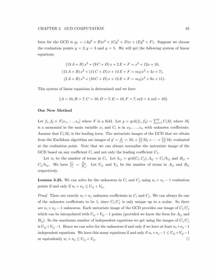
CHAPTER 3. GCD COMPUTATION 85
form for the GCD is gf = (Ay6 + B)x2 + (Cy7 + D)x + (Ey9 + F ). Suppose we choose
the evaluation points y = 2, y = 3 and y = 5. We will get the following system of linear
equations.
(13A+B)x2 + (9C +D)x+ 2E + F = x2 + 12x+ 10,
(15A+B)x2 + (11C +D)x+ 14E + F = m2(x2 + 4x+ 7),
(2A+B)x2 + (10C +D)x+ 12E + F = m3(x2 + 9x+ 11).
This system of linear equations is determined and we have
A = 10, B = 7, C = 10, D = 7, E = 10, F = 7,m2 = 4,m3 = 10.
Our New Method
Let f1, f2 ∈ F [x1, . . . , xn] where F is a field. Let g = gcd(f1, f2) =∑T
i=1CiMi where Mi
is a monomial in the main variable x1 and Ci is in x2, . . . , xn with unknown coefficients.
Assume that C1M1 is the leading term. The univariate images of the GCD that we obtain
from the Euclidean algorithm are images of g′ = gC1
= M1 + C2C1M2 + · · ·+ CT
C1MT evaluated
at the evaluation point. Note that we can always normalize the univariate image of the
GCD based on any coefficient Ci and not only the leading coefficient C1.
Let ni be the number of terms in Ci. Let hij = gcd(Ci, Cj), Aij = Ci/hij and Bij =
Cj/hij . We have CiCj
=Aij
Bij. Let Uij and Vij be the number of terms in Aij and Bij
respectively.
Lemma 3.25. We can solve for the unknowns in Ci and Cj using ni + nj − 1 evaluation
points if and only if ni + nj ≤ Uij + Vij .
Proof. There are exactly ni + nj unknown coefficients in Ci and Cj . We can always fix one
of the unknown coefficients to be 1, since Ci/Cj is only unique up to a scalar. So there
are ni + nj − 1 unknowns. Each univariate image of the GCD provides one image of Ci/Cj
which can be interpolated with Uij +Vij − 1 points (provided we know the form for Aij and
Bij). So the maximum number of independent equations we get using the images of Ci/Cj
is Uij+Vij−1. Hence we can solve for the unknowns if and only if we have at least ni+nj−1
independent equations. We have this many equations if and only if ni+nj−1 ≤ Uij+Vij−1
or equivalently ni + nj ≤ Uij + Vij .

CHAPTER 3. GCD COMPUTATION 86
Lemma 3.26. We will have enough independent equations to solve for all the unknowns in
the form of the GCD if there exist 1 ≤ i 6= j ≤ T such that ni + nj ≤ Uij + Vij
Proof. Suppose for 1 ≤ i 6= j ≤ T we have ni + nj ≤ Uij + Vij . We can scale the images of
the GCD based on the j’th coefficient to obtain univariate images of
gf =C1
CjM1 + · · ·+ Cj−1
CjMj−1 +Mj +
Cj+1
CjMj+1 + · · ·+ CT
CjMT .
Since ni + nj ≤ Uij + Vij , using Lemma 3.25 we can solve for the unknown coefficients in
Ci and Cj . Then we can multiply each univariate image by the image of Cj and solve for
every unknown in Ck independently using the integer coefficients of the univariate images
of the GCD.
Lemma 3.26 is a special case of the following theorem.
Theorem 3.27. We will have enough independent equations to solve for all the unknowns
in the form of the GCD if and only if there exist S = i1, i2, . . . , ik ⊆ 1, 2, . . . , T such
that ij’s are distinct and
k∑j=1
(nij )− 1 ≤k∑j=2
(Uiji1 + Viji1 − 1).
Proof. Suppose for the set S = i1, i2, . . . , ik ⊆ 1, 2, . . . , T, we have∑k
j=1 (nij ) − 1 ≤∑kj=2 (Uiji1 + Viji1 − 1). Suppose we scale the univariate images of the GCD based on i1’th
coefficient. For each J ∈ S − i1, the J ’th coefficient in the GCD will contribute at most
(UJi1 + VJi1 − 1) independent equations. Also the equations that we get from two different
coefficients in the GCD are independent because they have different unknowns. Hence
the total number of equations that we get from the coefficients with indices in S − i1is∑k
j=2 (Uiji1 + Viji1 − 1) which is greater than the total number of unknowns which is∑kj=1 (nij ) − 1 and hence we can solve for all the unknowns in CJ , where J ∈ S and
then solve the linear systems for the rest of coefficients (with indices in 1, 2, . . . , T − S)
independently. Conversely, for k = T , we have∑T
j=2 (Uiji1 + Viji1 − 1) is the maximum
number of independent equations that we get using the univariate images, no matter how
many evaluation points, thus if we can solve for the unknowns in the form gf we have∑Tj=1 (nij )−1 ≤
∑Tj=2 (Uiji1 + Viji1 − 1). Thus S = 1, 2, . . . , T satisfies the condition.
Using Theorem 3.27 we can compute a bound on the number of evaluation points we
need in order to solve for all the unknowns in the form of the GCD.

CHAPTER 3. GCD COMPUTATION 87
Theorem 3.28. If the requirement in Theorem 3.27 is satisfied, that is if there exist S =
i1, i2, . . . , ik ⊆ 1, 2, . . . , T such that all ij’s are distinct (∀ 1 ≤ j ≤ k) and
(
k∑j=1
nij )− 1 ≤k∑j=2
(Uiji1 + Viji1 − 1),
then using 2nmax − 1 evaluation points, we can solve for all the unknowns.
Proof. The proof is straight forward. Suppose for S = i1, i2, . . . , ik the requirement is
satisfied. Let βJ = UJi1 + VJi1 − 1 for J ∈ S − i1. Without loss of generality assume
βi1 ≤ βi2 ≤ · · · ≤ βik . Using N images, the J ’th coefficient will contribute min(βJ , N)
independent evaluations, hence the total number of equations would be
min(βi1 , N) + min(βi2 , N) + . . . ,min(βik , N)
hence For N = βik , the number of equations will be
βi1 + βi2 + · · ·+ βik =k∑j=2
(Uiji1 + Viji1 − 1)
which is greater than or equal to the number of unknowns which is∑k
j=1 (nij ) − 1 hence
using βk evaluation points we can solve for the unknowns in the coefficients of gf with
indices in S. Hence the total number of evaluation points needed is max(βk, nmax). There
are two cases. First assume βk > ni1 + nk − 1. In this case, we can use only the i1’th and
k’th coefficient of the GCD to solve for the unknowns in Ci1 and then scale the univariate
images based on the image of Ci1 and solve the rest of the linear systems independently,
hence the total number of images needed would be max(ni1 + nk − 1, nmax) ≤ 2nmax − 1.
Now if βk ≥ ni+1 + nk − 1, then βk ≤ 2nmax − 1, hence the total number of evaluations
needed is max(βk, nmax) ≤ 2nmax − 1.
The proof of Theorem 3.28 is constructive. The following is an example of our new
method.
Example 3.29. Let p = 17 be the prime and g = (y2 +1)x2−(y3 +y)x+(y3−2y+7) be the
same GCD as in Example 3.23. Here n1 = n2 = 2 and n3 = 3. We have C2C1
= y so U21 = 1
and V21 = 1. We have n1 +n2 = 4 > U12 +V12 so we can not use C1 and C2 to solve for the
leading coefficient. But C3C1
= y3−2y+7y2+1
so U31 = 3 and V31 = 2 hence n1 +n3 = 5 ≤ U31 +V31.

CHAPTER 3. GCD COMPUTATION 88
Thus we can scale the univariate images based on the first coefficient and use the images
of the third coefficient to solve for the unknowns in C1 and C3. The form for the GCD
is gf = (A1y2 + A2)x2 + (A3y
3 + A4y)x + (A5y3 + A6y + A7). We need n1 + n3 − 1 = 4
equations. Suppose we choose the evaluation points y = 1, y = 7, y = 14 and y = 15. The
four univariate images are
g1 = x2 + 16x+ 3,
g2 = x2 + 10x+ 4,
g3 = x2 + 3x+ 2,
g4 = x2 + 2x+ 4.
We fix A1 = 1. Using the third integer coefficients in the above images we get the following
set of equations
A5 +A6 +A7
1 +A2= 3⇒ A5 +A6 +A7 − 3A2 = 3,
3A5 + 7A6 +A7
1 + 15A2= 4⇒ 3A5 + 7A6 +A7 − 9A2 = 4,
7A5 + 14A6 +A7
1 + 9A2= 2⇒ 7A5 + 14A6 +A7 −A2 = 2,
9A5 + 15A6 +A7
1 + 4A2= 4⇒ 9A5 + 15A6 +A7 − 16A2 = 4.
After solving the above system of linear equations we obtain:
A2 = 1, A5 = 1, A6 = 15, A7 = 7,
hence the leading coefficient is C1 = y2 + 1. We scale the univariate images based on the
leading coefficient C1 evaluated at the corresponding evaluation points to obtain
g′1 = g1 × (1 + 1) = 2x2 + 15x+ 6,
g′2 = g2 × (72 + 1) = 16x2 + 7x+ 13,
g′3 = g3 × (142 + 1) = 10x2 + 13x+ 3,
g′4 = g4 × (152 + 1) = 5x2 + 10x+ 3.

CHAPTER 3. GCD COMPUTATION 89
To solve for the unknowns in C2 we get the following equations
A3 +A4 = 15,
3A3 + 7A4 = 7,
7A3 + 14A4 = 13,
9A3 + 15A4 = 10.
Solving the above system results in
A3 = A4 = 16
hence the GCD is (y2 + 1
)x2 + 16
(y3 + y
)x+ y3 + 15 y + 7
and we are done.
Now we can use Zippel’s idea in [85] to choose the evaluation points carefully so that
each system of linear equations will be a transposed Vandermonde system. One can invert
a Vandermonde matrix in O(n2) time and O(n) space compared to O(n3) time and O(n2)
space for a general matrix. Let α = (α2, α3, . . . , αn) where αi ∈ Zp. Let g ∈ F [x1, . . . , xn]
be the GCD that we wish to compute. We choose
αi = (x2 = αi2, x3 = αi3, . . . , xn = αin)
as the (i+1)’th evaluation point, i.e. the first evaluation point is α0 = (x2 = 1, . . . , xn = 1),
the second evaluation point is α1 = (x2 = α2, . . . , xn = αn) and so on. Assume that we
have scaled the univariate images of the GCD based on the j’th coefficient. Using this idea,
after solving the first system of equations to compute the unknowns for Cj and multiplying
univariate images by the image of Cj at the corresponding evaluation point, the rest of
linear systems will be transposed Vandermonde systems. We can solve them in quadratic
time, linear space and in parallel.
Example 3.30. Let p = 17 and g = (yu3 + 14y2u2)x3 + (3y2 + 4u − 8)x2 + (12y3u3 −7y2u+ 14u− 3)x+ (2u− v). We have gf = (A1yu
3 +A2y2u2)x3 + (A3y
2 +A4u+A5)x2 +
(A6y3u3 +A7y
2u+A8u+A9)x+ (A10u+A11v). If we scale the images based on the leading
coefficient yu3 +14y2u2 then we can use the fourth coefficient C4 and solve for the unknowns

CHAPTER 3. GCD COMPUTATION 90
in C1 and C2 using three equations. Since nmax = n3 = 4 we need at least four evaluation
points. Suppose we choose the evaluation points to be α0 = (y = 1, u = 1), α1 = (y = 2, u =
3), α2 = (y = 4, u = 9) and α4 = (y = 8, u = 33 mod 17 = 10).
Suppose we have computed C1 = yu3 + 14y2u2 and C4 = 2u − v. The system of linear
equations for C2 and C3 are 1 1 1
4 3 1
16 9 1
=
1 1 1
a b c
a2 b2 c2
and
1 1 1 1
12 12 3 1
8 8 9 1
11 11 10 1
=
1 1 1 1
a b c d
a2 b2 c2 d2
a3 b3 c3 d3
respectively.
A Problem
Suppose the univariate images of the GCD are scaled based on the i’th coefficient Cj . The
evaluation point αi is said to be bad, if Cj(αi) = 0. If αi is bad, then we can not scale the
univariate image of the GCD based on Cj .
Example 3.31. Let g = (uy4 + 10uy2 + 9u)x2 + (14uy3 + 2uy+ 11y+ 4)x+ 6u3 + 4uy and
p = 17. Suppose we are scaling the univariate images based on C2. We can not use the
evaluation point α1 = (y = 2, u = 3) because C2(α1) mod 17 = 0. The univariate image of
the GCD evaluated at α1 is g1 = x2 + 2.
We must avoid using a bad evaluation point. But unfortunately, unless we are scaling
based on the leading coefficient (or the trailing coefficient), detecting a bad evaluation point
beforehand can not be done easily. If we encounter a bad evaluation point we can either scale
the univariate images based on a different coefficient or we can throw away this evaluation
point and start with a new one. We do the latter.
Remark 3.32. Based on Theorem 3.28, if we can get enough independent equations to solve
for all the unknowns in gf , then having 2nmax−1 equations is sufficient to have determined

CHAPTER 3. GCD COMPUTATION 91
systems of linear equations. Thus in our algorithm if using 2nmax − 1 equations does not
lead to a determined system of linear equations, we assume that a previous choice of prime
or evaluation point is unlucky and restart the algorithms with a new prime or evaluation
points.
Benchmarks
We have implemented SparseModGcd algorithm both with and without the optimizations
discussed in this chapter in Maple 13. We will compare the performances of these algorithms
on two sets of benchmarks given in [30]. The polynomials in the first set have sparse GCDs
while the GCDs of the polynomials in the second set are completely dense. All timings are
in CPU seconds and were obtained using Maple 13 on a 64 bit Intel Core i7 920 @ 2.66GHz,
running Linux, using 31.5 bit primes.
SPARSE-1
Let m(z) = z3 − (s + r)z2 − (t + v)2z − 5 − 3u. For n = 1, 2, . . . , 10, let f1 = a × g and
f2 = b× g where
g = sxn1 + txn2 + uxn3 +4∑j=1
n−1∑i=0
r(1)ijzj−1xij +
∑w=[r,s,t,u,v]
n∑k=0
r(1)wkwk,
a = txn1 + uxn2 + sxn3 +4∑j=1
n−1∑i=0
r(2)ijzj−1xij +
∑w=[r,s,t,u,v]
n∑k=0
r(2)wkwk,
b = uxn1 + sxn2 + txn3 +4∑j=1
n−1∑i=0
r(3)ijzj−1xij +
∑w=[r,s,t,u,v]
n∑k=0
r(3)wkwk
and each r(i)jk
is a positive random integer less than 100. Thus we have 10 GCD problems,
all with one field extension m(z), five parameters r, s, t, u and v and four variables x1, x2, x3
and x4. Each input polynomial is of degree 2n in the first three variables and 2n− 2 in x4.
We wanted a data set of polynomials which are sparse but not too sparse. Also the GCD
g is sparse (g has 9n + 3 terms and deg(g) = n in any of x1, x2 and x3). The timings are
given in Table 3.2.

CHAPTER 3. GCD COMPUTATION 92
Table 3.2: Timings (in CPU seconds) for SPARSE-1
n SparseModGcd Optimized SparseModGcd Speedup (percentage)10 12.087 10.975 10.13%15 39.315 34.879 12.71%20 95.554 85.683 11.52%25 196.126 176.651 11.02%30 368.859 329.680 11.88%35 641.733 571.149 12.35%40 1007.663 938.878 7.32%45 1528.628 1426.273 7.17%50 2278.426 2178.779 4.57%
DENSE-1
Let m(z) = z2 − sz − 3. Suppose g, a and b are three randomly chosen polynomials in
x1, x2, s and z of total degree n which are dense. That is, the term xd11 xd22 s
d3zd4 with
0 ≤ d1 + d2 + d3 + d4 ≤ n is present in each of these three polynomials. So each has exactly∑ni=0
(i+4
4
)terms before we reduce by m(z). For n = 5, 6, . . . , 10, 15, 20, 30, let f1 = g × a
and f2 = g × b. The timings are given in Table 3.3.
Table 3.3: Timings (in CPU seconds) for DENSE-1
n SparseModGcd Optimized SparseModGcd Speedup (percentage)5 0.202 0.147 37.41%6 0.360 0.227 58.59%7 0.584 0.359 62.39%8 0.861 0.553 57.14%9 1.326 0.747 77.51%10 2.297 1.398 64.30%15 13.311 7.098 87.53%20 60.029 27.927 114.94%30 521.690 239.638 117.70%
The data in Tables 3.2 and 3.3 show that our optimized algorithm has a better per-
formance compared to the old algorithm especially for dense polynomials. This is because
for dense polynomials, the bottleneck of the algorithm is trial divisions in both zero and
non-zero characteristic.

Chapter 4
Factorization
In a computer algebra system, computations with polynomials over algebraic function fields
such as computing GCDs and factorization arise, for example, when one solves non-linear
polynomial equations involving parameters.
There are various algorithms for factoring polynomials over an algebraic number or
function field L. We discussed some of these algorithms in Section 1.3.3.
Our main focus in this chapter is factoring multivariate polynomials in L[x1, . . . , xv]
using Hensel lifting. We evaluate all parameters and all variables except one at small
integers thus reducing the factorization in L[x1, . . . , xv] to univariate factorization in x1 over
a number ring. There are a number of efficient algorithms for univariate factorization [67, 47,
52]. We choose to use Trager’s algorithm [67] because it is highly effective in implementation
for the fields and degrees we are interested in. We choose the evaluation point α ∈ Zk such
that L(α), the number ring obtained by evaluating the parameters t1, . . . , tk in L at α, is a
field.
When one uses Hensel lifting, a challenge is to solve the leading coefficient problem for
lifting non-monic polynomials. Abbott in [1], suggests using a trick by Kaltofen in [38]
which recursively computes the leading coefficients from their bivariate images using Hensel
lifting. Our approach is to modify Wang’s ingenious method given in [77] for factoring
polynomials over Z. Let f ∈ Z[x1, . . . , xv]. His idea is to first factor the leading coefficient
l(x2, . . . , xv) = lcx1(f) of the input polynomial f in the main variable x1, recursively. Then
evaluate all the variables except x1 at an evaluation point α ∈ Zv−1 and factor the univariate
polynomial f(x1, α). Now using the integer leading coefficients of the univariate factors, one
can determine which factor of l(x2, . . . , xv) belongs to the leading coefficient of which factor
93

CHAPTER 4. FACTORIZATION 94
of f(α). To do this, Wang identifies unique prime divisors for each factor of l(x2, . . . , xv)
evaluated at α by computing integer GCDs only. Unfortunately this idea does not generalize
to L. We show an example.
Example 4.1. Let L = Q(√−5) and
f = ((y +√−5 + 1)x+ 1)((y +
√−5− 1)x+ 1)
= (y2 + 2√−5y − 6)x2 + 2(y +
√−5)x+ 1.
We have lcx(f) = y2 + 2√−5y − 6 ∈ L[y], so if we evaluate y at α ∈ Z, we will obtain an
element of Z[√−5]. But Z[
√−5] is not a unique factorization domain thus GCDs do not
always exist in this ring. For example, for y = 0 we have lcx(f)(y = 0) = −6 = −2 × 3 =
−(1−√−5)× (1 +
√−5).
An easy solution to the leading coefficient problem is to make the input polynomial monic
by shifting the variables x2, . . . , xv. We illustrate with an example.
Example 4.2. In Example 4.1, if we substitute y = x+ 2y in f , we will obtain
f = f(x, x+ 2y) = (x2 + 2xy +√−5x+ x+ 1)(x2 + 2xy +
√−5x− x+ 1) =
x4 + 4 yx3 − 4x2 + 4 y2x2 + 4 yx+(2x3 + 4 yx2 + 2x
)√−5 + 1.
We have lcx(f) = 1. One can obtain factors of f by substituting y = x − 2y in the factors
of f . The problem with this solution is that it could make the input polynomial f denser.
Another problem is that one needs to do computations with fractions in Hensel lifting.
To solve this problem, one can work modulo pl, a power of a prime. This modulus, pl,
must be at least twice the largest integer coefficient in any factor of f . Unfortunately the
known bounds on the sizes of the integer coefficients in the factors of f are usually very
big which makes the computations really slow. In [1] it is suggested that it is better not
to do the calculations modulo pl because of the bad bounds but instead to lift over Q. In
our algorithm we choose a prime p of a modest size and then lift the integer coefficients to
their correct values using a new multivariate p-adic lifting algorithm which uses a sparse
interpolation method similar to Zippel’s algorithm [84].
This chapter is organized as follows. In Section 4.1 we present an example showing the
main flow and the key features of our algorithm. We then identify possible problems that

CHAPTER 4. FACTORIZATION 95
can occur and how the new algorithm deals with them in Section 4.2. In Section 4.3 we
present our new algorithm. Finally, in Section 4.4 we compare Maple implementations of
our algorithm with Trager’s algorithm for a set of polynomials.
4.1 An Example
Let F = Q(t1, . . . , tk), k ≥ 0. For i, 1 ≤ i ≤ r, let mi(z1, . . . , zi) ∈ F [z1, . . . , zi] be monic and
irreducible over F [z1, . . . , zi−1]/ 〈m1, . . . ,mi−1〉. Let L = F [z1, . . . , zr]/ 〈m1, . . . ,mr〉. L is
an algebraic function field in k parameters t1, . . . , tk (this also includes number fields). Let
f be a non-zero square-free polynomial in L[x1, . . . , xv]. Our problem is given f , compute
f1, f2, . . . , fn such that f = lcx1,...,xv(f)× f1 × f2 × · · · × fn where fi is a monic irreducible
polynomial in L[x1, . . . , xv].
Our algorithm works with the monic associate f of the input f and primitive associates
of the minimal polynomials which we now define.
Definition 4.3. Let D = Z[t1, . . . , tk]. A non-zero polynomial in D[z1, . . . , zr, x1, . . . , xv]
is said to be primitive wrt (z1, . . . , zr, x1, . . . , xv) if the GCD of its coefficients in D is
1. Let f be non-zero in L[x1, . . . , xv]. The denominator of f is the polynomial den(f) ∈ Dof least total degree in (t1, . . . , tk) and with smallest integer content such that den(f)f is
in D[z1, . . . , zr, x1, . . . , xv]. The primitive associate, f = prim(f), of f is the associate of
den(f)f which is primitive in D[z1, . . . , zr, x1, . . . , xv] and has positive leading coefficient
in a term ordering. The monic associate f of f is defined as f = prim(monic(f)). Here
monic(f) is defined by lcx1,...,xv(f)−1f .
Example 4.4. Let f = 3tx2 + 6tx/(t2 − 1) + 30tz/(1− t) where m1(z) = z2 − t. Here
f ∈ L[x] where L = Q(t)[z]/⟨z2 − t
⟩is an algebraic function field in one parameter t. We
have den(f) = t2 − 1 and f = prim(f) = den(f)f/(3t) = (t2 − 1)x + 2x − 10z(t + 1). For
f = 2zx2 + 2/t we have prim(f) = tzx2 + 1, monic(f) = x2 + z/t2 and f = t2x2 + z.
We demonstrate our algorithm using the following example using t for a parameter and
x and y for variables.
Example 4.5. Let m(z) = z2 − t3 + t and
f = (t3 − t)y2x2 + (20t3z − t2z − 20tz + z)yx2+
(−20t5 + 40t3 − 20t)x2 + (−tz + 21z)yx+ (421t3 − 421t)x− 21t

CHAPTER 4. FACTORIZATION 96
=1
t2 − 1× f1 × f2 =
1
t2 − 1((t2 − 1)xy + (t2 − 1)20zx− z)((t3 − t)xy − (t2 − 1)zx+ 21z)
= (t3 − t)(xy + 20zx− z
t2 − 1)(xy − zx
t+
21z
t3 − t).
Here L = Q(t)[z]/⟨z2 − t3 + t
⟩and f ∈ L[x, y]. We have prim(f) = f and m = m. The first
step in our algorithm is to eliminate any algebraic elements in γ = lcx,y(prim(f)) = t3 − tby computing f . This is done to avoid any fractions in the parameter t in the Hensel lifting.
Since γ does not involve the algebraic element z, we have f = prim(f).
Suppose we choose x as the main variable. In order to use Hensel lifting we factor the
leading coefficient
lcx(f) = (t3 − t)y2 + (20t3z − t2z − 20tz + z)y − 20t5 + 40t3 − 20t.
We do this by recursively using our algorithm in one less variable. The base case, for
univariate polynomials over a number field, is done by using Trager’s algorithm [67]. We
will obtain
lcx(f) = γ × l1 × l2 = (t3 − t)(y − z/t)(y + 20z).
Now we clear the denominators in li’s to obtain lcx(f) = γ× l1× l2 = (t2−1)(ty−z)(y+20z).
In order to factor f , we evaluate it at a point α for all the parameters and variables except
the main variable, x. We factor the resulting univariate polynomial in Q[z][x]/ 〈m(α)〉 using
Trager’s algorithm and then we lift the variables and parameters one by one using Hensel
lifting. Suppose we choose the evaluation point to be α = (t = 12, y = 5). This evaluation
point must satisfy certain conditions that we will discuss in Section 4.2.2. We have
f(α) = (170885z − 4864860)x2 + (45z + 722436)x− 252
and m(α) = z2 − 1716 which is irreducible hence L(α) is a field, one condition on α. Using
Trager’s algorithm, we factor f(α) over L(α) to get f(α) = lcx(f(α))× u1 × u2 with u1, u2
monic. We obtain
f(α) = (170885z − 4864860)× (x+1
19630325z − 48
137275)× (x+
105
22451z +
21
157).
We next factor γ = t2 − 1 over Z to obtain γ = t2 − 1 = l3 × l4 = (t − 1)(t + 1). Before
doing Hensel lifting, we determine the true leading coefficient of each factor of f in Z[t][y].
To do this, we use the denominators of u1 and u2. We know that
di = den(ui) | den(1
lcx(fi(α)))

CHAPTER 4. FACTORIZATION 97
where fi is a factor of f . We have
d1 = den(u1) = 19630325 = (5)2(11)(13)(17)2(19),
d2 = den(u2) = 22451 = (11)(13)(157),
D1 = den(1/l1(α)) = 1884 = (2)3(3)(157) where l1 = ty − z,
D2 = den(1/l2(α)) = (5)2(17)2(19) where l2 = y + 20z,
D3 = den(1/l3(α)) = 11 where l3 = t− 1,
D4 = den(1/l4(α)) = 13 where l4 = t+ 1.
The evaluation point α was chosen so that Di’s have a set of distinct prime divisors, namely
3, 17, 11, 13. Here Di’s are relatively prime so we have
gcd(di, Dj) > 1⇒ lj | li
where li = lcx1(fi). Using this we obtain l1 = (t2− 1)(y+ 20z) and l2 = (t2− 1)(ty− z) and
we have
f ≡ 1
t2 − 1× (l1(α)u1)× (l2(α)u2) mod 〈t− 12, y − 5〉 .
To avoid fractions in Q(t) in the Hensel lifting we multiply
f :=l1 × l2lcx1(f)
× f = (t2 − 1)× f
and use this new f in Hensel lifting. Now we use Hensel lifting to lift the parameter t and
the variable y in the other coefficients of the fi. To avoid any computations with fractions
in Q, we do the calculations modulo a prime, say p = 17. After applying Hensel lifting
we obtain the factors f1 = ((t2 − 1)(y + 20z)x − z) and f2 = ((t2 − 1)(ty − z)x + 4z) s.t.
f ≡ f1 × f2 (mod 17). The final task is to find the integer coefficients of f1 and f2 so that
f = f1 × f2. To do this, we use sparse interpolation. We have e1 = f − f1 × f2 mod 〈m〉,the first error polynomial over Z. We want to find σ1, σ2 ∈ L[x, y] such that
f ≡ (f1 + σ1 × p)(f2 + σ2 × p) mod p2.
Assuming that our choice of α and p has not caused any terms in the polynomials f1 and
f2 to vanish, we know that the monomials in σ1 and σ2 are the same as those in f1 and
f2 respectively, so we have the assumed forms for σ1 and σ2. If p is large and α is chosen
randomly, this would happen with high probability. Since f1 and f2 have correct leading

CHAPTER 4. FACTORIZATION 98
coefficients we have σ1 = Az and σ2 = Bz for unknown integer coefficients A and B. To
find the values for A and B we have
(σ1 × f2 + σ2 × f1) mod 〈m〉 − e1
p≡ 0 mod p.
After equating every coefficient in monomials in x, y, z and t in the above expression to zero,
we get the following linear system:
A = 0,−B + 1 = 0, B − 1 = 0,−1− 4A+B = 0, 1−B + 4 = 0,
A = 0,−A− 20 + 20B = 0, 2A+ 40− 40B = 0,−A = 0.
Solving modulo p, we get A = 0 and B = 1 so we update
f1 := f1 + σ1 × p = ((t2 − 1)(y + 20z)x− z)
and
f2 := f2 + σ2 × p = ((t2 − 1)(ty − z)x+ 21z).
Now we have f ≡ f1× f2 mod p2. This time the new error e2 = f − f1× f2 mod 〈m〉 is zero,
so we have
f = f1 × f2 = ((t2 − 1)xy + (t2 − 1)20zx− z)((t3 − t)xy − (t2 − 1)zx+ 21z).
To complete the factorization of f we have f = lcx,y(f)×monic(f1)×monic(f2), thus
f = (t3 − t)(xy + 20zx− z
t2 − 1)(xy − zx
t+
21z
t3 − t)
and we are done.
4.2 Problems
In the example we mentioned that the evaluation point must satisfy certain conditions in
order for the algorithm to work properly. Another issue is the defect of the algebraic function
field L which is the biggest denominator of any algebraic integer in L (See [1, 81]). Here we
identify all problems.

CHAPTER 4. FACTORIZATION 99
4.2.1 The Defect
Unlike factorization over Q, when factoring a polynomial f over the algebraic field L, the
leading coefficient of a factor fi in the variables x1, . . . , xv might not divide the leading
coefficient of f , i.e. lcx1,...,xv(fi) - lcx1,...,xv(f) in Z[t1, . . . , tk].
Example 4.6. Let m = z2 − t3, L = Q(t)[z]/ 〈m〉 and f = x2 − t. We have f = f and
f = (x− z
t)(x+
z
t) =
1
t2(tx− z)(tx+ z).
Here f1 = tx− z but lcx(f1) = t - lcx(f) = 1.
The denominator t in this example is a divisor of the defect of the algebraic function field
L. The defect is the largest rational integer that divides the denominator of any algebraic
integer in the field (See e.g. [6]).
Theorem 4.7 (See Abbott [1]). Let ∆ ∈ Z[t1, . . . , tk] be the discriminant of the algebraic
field L. The defect is the biggest square that divides ∆.
Example 4.8. When r = 1 (one field extension), ∆ = resz1(M,M ′) where M = m1. For
example, for m1 = z21 − t3 we have ∆ = resz1(z2
1 − t3, 2z1) = −4t3 and hence 2t is the defect.
Theorem 4.9 (See Abbott [1]). Let di = degzi(mi). The discriminant of L is
∆ =r∏i=1
N1(N2(. . . (Ni−1(discr(mi)di+1...dr)) . . . ))
where Ni(f) = reszi(f, mi) and discr(mi) = reszi(Mi,M′i) where Mi = mi.
Suppose using Theorem 4.9 we have computed the discriminant ∆ ∈ Z[t1, . . . , tk]. Let
δ×De11 × · · · ×D
ekk be a square-free factorization of ∆ where δ ∈ Z. Since we want to avoid
integer factorization, we choose D to be this integer multiple of the defect:
D = δ ×Dbe12c
1 × · · · ×Dbek2c
k .
Theorem 4.10 (See [81]). If fi is a factor of f and D is an integral multiple of the defect,
then
lcx1,...,xv(fi) | D× lcx1,...,xv(f).
Remark 4.11. In this chapter, we always assume the lexicographic monomial ordering with
x1 > x2 > · · · > xv.

CHAPTER 4. FACTORIZATION 100
Remark 4.12. The leading coefficient of f , lcx1,...,xv(f) ∈ Z[t1, . . . , tk], may not split
among the leading coefficients of the factors. That is∏ni=1 lcx1,...,xv(fi) may not divide
Dl × lcx1,...,xv(f) for any l ∈ Z+.
Example 4.13. In Example 4.5, the discriminant of L is −4t3 + 4t and hence D = 4. We
have lcxf = t3− t, lcxf1 = t2− 1 and lcxf2 = t3− t. We have (t2− 1)× (t3− t) - Dl× (t3− t)for any l ∈ Z+.
4.2.2 Good and Lucky Evaluation Points
Definition 4.14 (Good Evaluation Points).
Let α = (t1 = α1, . . . , tk = αk, x2 = β2, . . . , xv = βv) ∈ Zk+v−1 be the evaluation point
that we choose in our algorithm to factor the univariate polynomial f(α). We impose the
following conditions on α. We say α is good if:
1. The leading coefficient of f in the main variable x1 and the leading coefficient of mi
in zi do not vanish after evaluating at α, i.e. degx1(f) = degx1(f(α)) and degzi(mi) =
degzi(mi(α)).
2. L(α) remains a field so that we still have unique factorization of f(α). As an example,
the evaluation point t = 1 is not a good choice for our Example 4.4 because the minimal
polynomial z2 − t evaluated at this point is no longer irreducible.
3. The polynomial f evaluated at α remains square-free in x1, i.e. gcd(f(α), f ′(α)) = 1
in L(α)[x1] , so that we can apply Hensel lifting.
4. The fourth condition on the evaluation point α enables us to distribute factors of
lcx1(f) to the monic univariate factors u1, . . . , un where ui ∈ L(α)[x1] and
f(α) = lcx1(f)(α)× u1 × · · · × un.
Suppose γ × le11 × · · · × lemm is the factorization of lcx1(f) over L and D is the defect.
Here γ ∈ Z[t1, . . . , tk] and l ∈ L[x2, . . . , xn]. Let β = D × γ = Ω × βc11 × βc22 ×· · · × βckk ∈ Z[t1, . . . , tk] where Ω ∈ Z and βi ∈ Z[t1, . . . , tk] is irreducible over Z. Let
di = den(1/li(α)). In order to be able to uniquely distribute the factors of D× lcx1(f)
to the univariate factors, we require that numbers in the set

CHAPTER 4. FACTORIZATION 101
A = β1(α), . . . , βk(α), d1, . . . , dm
have distinct prime divisors that do not divide Ω (See Example 4.15 below).
Also, a prime p is considered to be a good prime if the leading coefficient of f in x1 and
the leading coefficient of mi(α) in zi do not vanish modulo p.
Example 4.15. In Example 4.5 we have β1 = t − 1, β2 = t + 1, l1 = ty − z, l2 = y + 20z,
D = 2 and Ω = 2. We can not use the evaluation point α = (t = 3, y = 5) because the
numbers in A = 2 = (2), 4 = (2)2, 417 = (3)(139), 9551 = (9551) do not have distinct
prime divisors.
Remark 4.16. Let lcx1(f) = γ × le11 × · · · × lemm where li is an irreducible factor of lcx1(f).
Let Ni = norm(li) ∈ Q(t1, . . . , tk)[x1, . . . , xv]. If ∃i 6= j such that Ni | Nj over Q(t1, . . . , tk)
then condition 4 may not be satisfied, no matter what α is. This especially happens if li
and lj are conjugates hence Ni = Nj . In this case, the denominators di = den(1/li(α)) and
dj = den(1/lj(α)) will be images of the same polynomial norm(li) = norm(lj) (See [67]).
Here we need to do something else. The simplest solution, as shown in Example 4.2 is to
shift the variables x2, x3, . . . , xv in the input polynomial by computing
f := f(x1, x1 + c2x2, x1 + c3x3, . . . , x1 + cvxv)
for some randomly chosen ci ∈ Z. Now lcx1(f) ∈ Z[t1, . . . , tk]. The the leading coefficient
of f in x1 will not involve any of the variables x2, x3, . . . , xv. The following is an example.
Example 4.17. Let m = z2− t and f = x2y2− tx2 +2txy+ t2 = ((y+z)x+ t)((y−z)x+ t).
We have lcx(f) = y2 − t = l1 × l2 = (y − z)(y + z) and norm(l1) = norm(l2) = y2 − t. If we
choose α = (y = 1, t = 6) we will have d1 = den(1/l1(α)) = 5 and d2 = den(1/l2(α)) = 5
and the set A = 5, 5 will not have a set of distinct prime divisors. If we shift the variable
y to x + 3y, we will get f := f(x, x + 3y) = (x2 + (3y + z)x + t)(x2 + (3y − z)x + t) and
lcx(f) = 1.
Definition 4.18 (Lucky Evaluation Point). A good evaluation point α ∈ Zv+k−1 is said to
be lucky if it satisfies the following conditions, otherwise it is unlucky.
(i) The number of irreducible factors of f(α) over L(α) is the same as the number of
irreducible factors of f over L.

CHAPTER 4. FACTORIZATION 102
(ii) If li | lcx1(fj) where fj is an irreducible factor of f then gcd(den(1/li(α)), lcx1(uj)) 6= 1.
(iii) If βi | lcx1(fj) then gcd(βi(α), lcx1(uj)) 6= 1
(iv) α does not annihilate any terms of any factor fi of f (See Example 4.19 below).
Similarly, a good prime p is said to be lucky if no terms of any factor fi of f is annihilated
modulo p. If the evaluation point α or prime p is unlucky, the algorithm must detect this
and restart using a new good evaluation point and a new good prime.
Example 4.19. Let f = f1× f2 where f1 = x2− (t−15)zx− tz+1 and f2 = x3−17tzx+1
where z =√t− 1. Here the evaluation point t = 15 is good but it is unlucky because it
annihilates the term (t − 15)zx in f1. Similarly, the prime p = 17 is unlucky because the
term 17tzx in f2 vanishes modulo p. Also, t = 0 is unlucky because f2(t = 0) factors but f2
does not.
Remark 4.20. Since we will use sparse interpolation to lift the integer coefficients of the
factors computed using Hensel lifting, the evaluation point α and the prime p must not
annihilate any terms in any factors of f . Unfortunately we will not be able to identify
unlucky evaluation points and primes in advance. Instead, if α is unlucky or p is unlucky
and the form of any of the correcting polynomials σ1, σ2, . . . is wrong, the system of linear
equations in the sparse interpolation will be inconsistent with high probability. To decrease
the probability of choosing an evaluation point (or a prime) that annihilates terms in factors
of f , one should choose α at random from a large set of evaluation points , e.g. p = 231 − 1
and α ∈ Zp at random.
Remark 4.21. If α is unlucky and there are extraneous factors in the factorization of f(α)
then Hensel lifting will fail with high probability. Hensel lifting may succeed modulo p with
low probability if the prime p in Hensel lifting is also unlucky and results in extraneous
factors in f mod p corresponding to those of f(α).
Example 4.22. Suppose f = x2 + 17(t− 1)zx− t2 and z =√t+ 1. The evaluation point
α = (t = 1) is good but unlucky because f is irreducible but f(α) = (x − 1)(x + 1). If we
also chose p = 17, Hensel lifting will succeed and return (x− t)(x+ t).
If Hensel lifting does not fail when α is unlucky, then we will not be able to lift the integer
coefficients of factors of f and the algorithm will restart by choosing a new evaluation point.

CHAPTER 4. FACTORIZATION 103
4.2.3 Degree Bound for the Parameters
In order to use Hensel lifting, we need to have bounds on the degrees of the parameters and
variables in the factors of f . For variables x1, . . . , xv we have degxi(f) =∑n
j=1 degxi(fj)
but unlike factorization over the rationals, degti(fj) is not necessarily bounded by degti(f).
Example 4.23. Let m = z2 − 1t3
and f = x2 − t. We have
f = f1f2 = (x+ t2z)(x− t2z).
Here degt f1 = degt f2 = 2 > degt f = 1.
In [1], Abbott gives a possible bound Ti on the degree of each factor in ti based on
Trager’s algorithm which is usually much bigger than the actual degrees of the factors. In
our algorithm when we lift the parameter ti in the factorization of f , as soon as the factors
have been lifted to the correct degree, the error would be zero (provided the evaluation point
and the prime are not unlike) and the algorithm succeeds. However if the evaluation point
is unlucky, our algorithm will have to lift the parameter ti to the degree Ti before realizing
it. But the probability that a randomly chosen evaluation point (from a large set of values)
is unlucky is low. Thus instead of using the bad bound Ti, we start the algorithm with a
heuristic bound T for the degree of the parameters. Now Hensel lifting fails if either the
evaluation point is unlucky or the heuristic bound T is not big enough. In this case, we will
double the heuristic bound, i.e. T := 2 × T , and restart the algorithm by choosing a new
evaluation point. In this way, we will eventually get both a good evaluation point and a big
enough bound T and Hensel lifting will eventually succeed.
In our implementation we choose the initial bound T based on the following conjecture
from Abbott [1]:
Conjecture 4.24 (Abbott [1]).
degti(fj) ≤ degti(f) +
r∑l=1
degti(ml).
4.2.4 Numerical Bound
Most algorithms that use Hensel lifting (See [82, 1]) either work over Q or work modulo a
power of a prime which must be larger than twice the size of the largest integer coefficients
in the factors of f . Abbott in [1] presents a bound for this but his bound is very poor. The
following is an example from [1].

CHAPTER 4. FACTORIZATION 104
Example 4.25. Let m = z2 − 4t− 1 and f = x2 + x− t = (x+ 1+z2 )(x+ 1−z
2 ). The bound
given by Abbott for factoring f is greater than 5000000.
The poor bound means a large modulus is needed which slows Hensel lifting down.
Instead, we work modulo a machine prime p and then lift the integer coefficients using our
sparse p-adic lifting algorithm if necessary. We still need a bound for the case where α is
unlucky and Hensel lifting has not detected this due to the unlucky choice of the prime p
(See Example 4.22). For this, we choose a heuristic bound B. Any good estimate for B
will work. Now if the sparse p-adic lifting fails, either α is unlucky or p is unlucky or the
bound B is not big enough. In this case, we square the bound, i.e. B := B2, and restart
the algorithm by using a new evaluation point α and new prime p. In this way, we will
eventually get a lucky evaluation point and a lucky prime and a bound big enough to lift
the integer coefficients.
4.3 The Algorithm
Algorithm 4.1: efactor
Require: f ∈ L[x1, x2, . . . , xv] where L is the algebraic function field.
Ensure: Factorization of f : f = l×fe11 ×· · ·×fenn where fi is a monic irreducible polynomial
and l = lcx1,...,xv(f).
1: If f ∈ L, return f .
2: Let c = contx1(f) ∈ L[x2, . . . , xn] be the content of f . If c 6= 1 then factor c and f/c
separately using Algorithm efactor and return their product.
3: Do a square-free factorization of f . Call Algorithm 4.2 on each square-free factor and
return the result.
Algorithm 4.2: Main Factorization Algorithm
Require: Square-free f ∈ L[x1, x2, . . . , xv] where contx1(f) = 1 and f /∈ L.
Ensure: Factorization of f : f = l×f1×f2×· · ·×fn where fi is monic and l = lcx1,...,xv(f).
1: Compute f (See Definition 4.3).
2: Compute D, an integral multiple of the defect of the algebraic field L See Theorem 4.9.

CHAPTER 4. FACTORIZATION 105
3: if v = 1 univariate case then
4: Call algorithm 4.4 on f and D and return the result.
5: end if
6: Choose a heuristic bound B for the largest integer coefficient in the factors of f .
7: Let T = maxki=1 (degti(f) +∑r
j=1 degti mj)
Heuristic bound on the degree of f in any parameter: Abbott’s conjecture 4.248: Factor lcx1(f) ∈ L[x2, . . . , xv] by calling algorithm efactor. Let lcx1(f) = γ × le11 × l
e22 ×
· · · × lemm where li is monic.
9: Compute li. Find γ, D ∈ Z[t1, . . . , tk] s.t. D × lcx1(f) = γ ×∏mi=1 lcx2,...,xv(li). Update
f := D × f . Note D | Dc for some c ∈ Z+.10: Let N be a counter initialized with zero.
11: Main Loop: Choose a new good evaluation point α = (t1 = α1, t2 = α2, . . . , tk =
αk, x2 = β2, . . . , xv = βv) at random that satisfies the requirements of Definition 4.14 in
Section 4.2.2. α1, . . . , αk, β2, . . . , βk ∈ Z\0.12: Using Trager’s algorithm factor f(α) over L(α) to obtain f(α) = Ω′×u1×· · ·×un where
Ω′ = lcx1(f)(α) ∈ Q[z1, . . . , zr]. If n = 1 then return l ×monic(f) f is irreducible13: Using Algorithm 4.6 on inputs u1, . . . , un, lcx1(f) = γ × le11 × le22 × · · · × lemm , the
evaluation point α, D and D1, . . . , Dm where Di = den(li(α)−1), compute the true
leading coefficients of each univariate factor l1, l2, . . . , ln. If this fails set N := N +
1. Note that f may be updated in order to distribute the integer content of D ×lcx1(f). If N < 10 then go to step 11 otherwise shift the variables x2, . . . , xv in f , call
Algorithm 4.2 recursively on the shifted f , and undo the shift in the factors and return.
See Example 4.17.14: Compute δ, l ∈ Z[t1, . . . , tk] s.t. δ× lcx1,...,xv(f) = l×
∏ni=1 lcx2,...,xv(li). δ | Dc for some
c ∈ Z+ and l is a factor of lcx1,...,xv(f) that is not in l1, . . . , ln.15: Set f := δf . At this point we have
f(α) = l(α)× (l1(α)u1)× · · · × (ln(α)un).
16: Choose a new good prime p satisfying lcx1(f(α)) mod p 6= 0, lczi(mi(α)) mod p 6= 0 and
f(α) is square-free modulo p.
17: Now we are set for Hensel lifting. Using Hensel lifting on inputs f , l, the set of univariate
images u1, . . . , un, the set of corresponding true leading coefficients l1, l2, . . . , ln, the
prime p, the bound T and the evaluation point α, lift the variables x2, x3, . . . , xv and

CHAPTER 4. FACTORIZATION 106
the parameters t1, . . . , tk to obtain f = l × f1 × f2 × · · · × fn mod 〈m1, . . . , mr, p〉 and
li = lcx1(fi).
18: If Hensel lifting fails then Set T := 2× T and go to Step 11.
19: Call algorithm 4.3 on inputs f , f1, f2, . . . , fn, l, the prime p, the bound B and the set
l1, l2, . . . , ln. If this fails, set B := B2 and go to step 11 otherwise let f ′1, f′2, . . . , f
′n be
the output s.t. f = l × f ′1 × · · · × f ′n over L.
20: return lcx1,...,xv(f)×monic(f ′1)× · · · ×monic(f ′n)
Algorithm 4.3: Sparse p-adic lifting
Require: f , f1, . . . , fn ∈ L[x1, . . . , xv], l ∈ Z[t1, . . . , tk] and p s.t. f− l× f1× f2×· · ·× fn =
0 mod 〈m1, . . . , mr, p〉. The numerical bound B and l1, . . . , ln the set of the leading
coefficients of the factors.
Ensure: Either FAIL, if the evaluation point is unlucky or polynomials h1, h2, . . . , hn s.t.
f = l × h1 × · · · × hn over L.
1: Let hi be fi with its leading coefficient replaced by li.
2: Let e = f − l×h1×· · ·×hn mod 〈m1, . . . , mr〉. Note that degx1(e) < degx1(f) because
we imposed lcx1(f) = l ×∏i=1 nhi
3: Let P = p.
4: Suppose fi =∑Ti
j=1 aijMij with aij ∈ Zp and Mij monomials.
5: Let σi =∑Ti
j=1AijMij where Aij is an unknown coefficient.
6: while e 6= 0 and P < 2B do
7: e′ = e/P exact integer division8: Let pz = e′ − l ×
∑ni=1 σi
∏nj=1 hjhi
mod 〈m1, . . . , mr〉.9: Solve for Aij ’s by collecting and equating coefficients of pz in x1, . . . , xv, t1, . . . , tk and
z1, . . . , zr to zero modulo P .
10: If the system of linear equations is inconsistent then return FAIL. Annihilated term
in the form due to the unlucky choice of p11: Update hi := hi + σi × P for 1 ≤ i ≤ n.
12: Set P := P 2
13: Set e = f − l × h1 × · · · × hn mod 〈m1, . . . , mr〉.14: end while
15: If e = 0 then return h1, h2, . . . , hn else return FAIL.

CHAPTER 4. FACTORIZATION 107
Algorithm 4.4: Univariate Factorization
Require: Square-free f ∈ L[x1] and D the defect of L.
Ensure: Unique factorization of f = lcx1(f)× f1 × f2 × · · · × fn over L s.t. fi is monic in
x1.
1: Compute f (See Definition 4.3) and Let l = lcx1(f).
2: Choose a heuristic bound B on the integer coefficients of the factors of f .
3: Let T = maxki=1 (degti(f) +∑r
j=1 degti mj)
Heuristic bound on the degree of f in any parameter: Abbott’s conjecture.4: Factor γ = D× l ∈ Z[t1, . . . , tk] over Z to obtain γ = Ω× βc11 × · · · × β
ck′k′ .
5: Main Loop: Choose a new good evaluation point α = (t1 = α1, . . . , tk = αk) that
satisfies the requirements of definition 4.14.
6: Using Trager’s algorithm, factor h = f(α) = l(α)×h1×h2× · · · ×hn over the algebraic
number field. Note that lcx1(hi) = 1.
7: Compute hi and let di = lcx1(hi) ∈ Z. Find the biggest eij s.t. βeiji | dj . Let li =
βe1i1 × · · · × βek′ik′ . Distribute Ω ∈ Z to li’s and if needed, update f and hi. At this point
we have li = lcx1(fi).
8: Compute δ, l ∈ Z[t1, . . . , tk] s.t. δ × l = l ×∏ni=1 li. δ | Dc for some c ∈ Z and l is a
factor of lcx1(f) that is not in l1, . . . , ln9: Let f = δf f(α) = l(α)× h1 × h2 × · · · × hn.
10: Choose a new good prime p satisfying lcx1(f(α)) mod p 6= 0, lczi(mi(α)) mod p 6= 0 and
f(α) is square-free modulo p.
11: Lift the parameters t1, . . . , tk in f(α)− l× h1× h2× · · · × hn ≡ 0 mod p using Hensel
lifting with li ∈ Z[t1, . . . , tk] as the true leading coefficient of hi and T as the degree
bound. If this fails, set T := 2× T and go to step 5 unlucky evaluation point.12: Call algorithm 4.3 on inputs f , h1, h2, . . . , hn, l, the prime p, l1, . . . , ln and B. If this
fails, set B := B2 and go to step 5 (main loop) otherwise let f ′1, f′2, . . . , f
′n be the output
s.t. f = l × f ′1 × · · · × f ′n over L.
13: return lcx1(f)×monic(f ′1)× · · · ×monic(f ′n).
Algorithm 4.5: Distinct prime divisors (Similar to Wang [77])
Require: A set a1, a2, . . . , an where ai ∈ Z.

CHAPTER 4. FACTORIZATION 108
Ensure: Either FAIL or a set of divisors d1, d2, . . . , dn ∈ Nn s.t. di 6= 1 and di | ai and
∀j 6= i : gcd(di, dj) = 1.
1: for i from 1 to n do
2: Let di = ai.
3: for j from 1 to i− 1 do
4: Let g = gcd(di, dj).
5: Set di := di/g and dj := dj/g.
6: Let g1 = gcd(g, di) and g2 = gcd(g, dj). Either g1 = 1 or g2 = 17: while g1 6= 1 do
8: Let g1 = gcd(di, g1).
9: Set di := di/g1.
10: end while
11: while g2 6= 1 do
12: Let g2 = gcd(dj , g2).
13: Set dj := dj/g2.
14: end while
15: if di = 1 or dj = 1 then
16: return FAIL.
17: end if
18: end for
19: end for
20: return d1, . . . , dn.
Algorithm 4.6: Distributing leading coefficients
Require: f and U = u1, u2, . . . , un, the set of monic univariate factors where ui ∈L(α)[x1]. l = γ × le11 × le22 × · · · × lemm the non-monic factorization of l = lcx1(f)
where γ ∈ Z[t1, . . . , tk]. The evaluation point α and D the defect of the algebraic field.
D1, . . . , Dm where Di = den(li(α)−1).
Ensure: Either FAIL, if the leading coefficient is unlucky or l1, l2, . . . , ln where li ∈L[x2, . . . , xv] is the true leading coefficient of ui in x1 together with possibly updated f .
1: Let β = D× γ = Ω× βc11 × βc22 × · · · × β
ck′k′ where Ω ∈ Z.
2: Let di = den(ui) and µi = βi(α).

CHAPTER 4. FACTORIZATION 109
3: Apply algorithm 4.5 on input [D1, . . . , Dm, µ1, . . . , µk′ ]. If Algorithm 4.5 fails, return
FAIL. Otherwise let p1, . . . , pm, q1, . . . , qk′ be the output.
4: For all 1 ≤ i ≤ m, let gi = gcd(Ω, pi) and Set pi := pi/gi. If pi = 1 then return FAIL.
5: For all 1 ≤ i ≤ k′, let g′i = gcd(Ω, qi) and Set qi := qi/g′i. If qi = 1 then return FAIL.
6: for each dj do
7: for i from 1 to m do
8: Let g1 = gcd(dj , pi).
9: Set e′ji = 0.
10: while g1 6= 1 do
11: Set e′ji := e′ji + 1.
12: Set dj = dj/g1.
13: Set g1 = gcd(dj , g1).
14: end while
15: end for
16: for i from 1 to k′ do
17: Let g2 = gcd(dj , qi).
18: Set c′ji = 0.
19: while g2 6= 1 do
20: Set c′ji := c′ji + 1.
21: Set dj = dj/g2.
22: Set g2 = gcd(dj , g2).
23: end while
24: end for
25: end for
26: for i from 1 to m do
27: if∑n
j=1 e′ji 6= ei then return FAIL.
28: end for
29: Let li = βci11 βci22 . . . βcik′k′ l
ei11 lei22 . . . leimm . Distribute Ω ∈ Z to lis and if needed update f .
30: return l1, l2, . . . , ln.
Remark 4.26. In our implementation of algorithm4.2, we first choose an evaluation point
and compute a univariate factorization then factor lcx1(f). This is because if f is irreducible,
then we do not bother factoring the leading coefficient which might be a big polynomial.

CHAPTER 4. FACTORIZATION 110
Description of Algorithm 4.3
The input to algorithm 4.3 is
f − l × f1 × f2 × · · · × fn ≡ 0 mod 〈p, m1, . . . , mr〉 .
Note, if mi is not monic, the reduction modulo m1, . . . , mr does not introduce fractions
in the parameters because of l. Let e1 = f − l × f1 × · · · × fn mod 〈m1, . . . , mr〉. We know
that p | e1. If e1 = 0 then we are done. We want to find polynomials σ1, . . . , σn s.t.
f − l × (f1 + σ1p)(f2 + σ2p) . . . (fn + σnp) ≡ 0 mod p2.
Expanding the above expression modulo 〈p, m1, . . . , mr〉 results in g ≡ 0 mod p where
g = l × (σ1f2f3 . . . fn + · · ·+ σnf1f2 . . . fn−1)− e
p.
We assume that the monomials in σi are the same as the monomials in fi with the integer
coefficient replaced by an unknown. We compute the polynomial g and equate each coef-
ficient in z1, . . . , zr, t1, . . . , tk, x1, . . . , xv to zero. This gives us a linear system which has a
unique solution because we already know the exact leading coefficient in the main variable
of each factor fi and uniqueness is guaranteed by Hensel’s lemma. After solving this system
we will obtain the correction polynomials σ1, . . . , σn. We update each factor fi := fi + σip.
Now we have
f − l × f1 × f2 × · · · × fn ≡ 0 mod p2.
We repeat this non-linear lifting algorithm until p2k > 2|B| where B is the heuristic bound
chosen in Algorithm 4.2 for the integer coefficients in the factors of f . Thus if there are no
extraneous factors and no annihilated terms caused by the choice of primes and evaluation
points, the algorithm will not depend on a bound on the size of the coefficients in the factor
of f which could be big.
Remark 4.27. In Step 8 of Algorithm 4.4 and Step 14 of algorithm 4.2, we compute
l ∈ Z[t1, . . . , tk] which is the factor of the leading coefficient of f in all the variables which
does not show up in the leading coefficient of any factors of f .
Remark 4.28. The bottleneck of Hensel lifting algorithm is solving the Diophantine equa-
tions. One can solve these Diophantine equations using sparse interpolation with a similar
technique as in algorithm 4.3. Here is an example.

CHAPTER 4. FACTORIZATION 111
Example 4.29. Let m = z2 − (t− 1)3 and
f =(t3 − t− t2 + 1
)x2 − x (2 t+ 1) z − t4 + t2.
Suppose we choose the evaluation point to be t = 4. We compute the univariate factors
using Trager’s algorithm and after computing and attaching the leading coefficients of the
factors we have
f = (t− 1)2f ,
f1 =(t3 − t− t2 + 1
)x+ 16 z,
f2 =(t2 − 2 t+ 1
)x− 5 z,
where f − f1f2 ≡ 0 mod (t− 4). Now we start Hensel lifting. The first error polynomial is
e1 = f − f1f2. We have
e1
t− 4=(3 t2z − 6 tz + 3 z
)x− t5 − 2 t4 − 8 t3 + 46 t2 − 55 t+ 20.
Now we need to find two polynomials σ1 and σ2 s.t.
σ2f1 + σ1f2 −e1
t− 4≡ 0 mod (t− 4). (4.1)
Similar to algorithm 4.3, we can assume that σ1 and σ2 have the same monomials as f1 and
f2 respectively and since we know that the leading coefficient of f1 and f2 are correct, the
forms for σ1 and σ2 are σ1 = Az and σ2 = Bz. Using these forms and Equation 4.1 we
construct and solve a linear system to obtain A = 8, B = −1. We update f1 := f1+σ1×(t−4)
and f2 := f2 + σ2 × (t− 4) to get
f1 = (t3 − t2 − t+ 1)x+ 16z + 8(t− 4)z,
f2 = (t2 − 2t+ 1)x− (t− 4)z − 5z.
This time the new error polynomial is e2 = f − f1f2 and we have
e2
(t− 4)2=(t2z − 2 tz + z
)x− t4 + 2 t3 − 2 t+ 1
and
σ2f1 + σ1f2 −e2
(t− 4)2≡ 0 mod (t− 4)2. (4.2)

CHAPTER 4. FACTORIZATION 112
The new assumed forms are
σ1 = Az +Bz(t− 4),
σ2 = Czt+Dz.
Again we construct a system of linear equations using Equation 4.2 and after solving this
system we have A = 1, B = 0, C = 0, D = 0. We update f1 and f2 and to obtain
f1 =(t3 − t2 − t+ 1
)x+ zt2,
f2 =(t2 − 2 t+ 1
)x− zt− z.
The new error polynomial e3 = f − f1f2 is zero so f = lcx(f)×monic(f1)×monic(f2) and
we are done.
We do not use this method in our new algorithm for lifting parameters and variables.
This is because it was always slower than solving the Diophantine equations using the
traditional method. The reasons are:
1. The systems of linear equations in each step can be very big if the factors are dense.
Example 4.30. Suppose f1, f2 and f1 × f2 have N1, N2 and N terms respectively.
Then the system of linear equation has N equations and as many as N1 − 1 +N2 − 1
unknowns.
2. As Hensel lifting progresses, usually, the error term gets smaller so solving the Dio-
phantine equation is usually easier at the next step. But using sparse interpolation,
as the Hensel lifting algorithm proceeds, each factor fi usually gets bigger because we
add new terms, so the system of linear equations gets bigger which makes the Hensel
lifting slower.
We do not have the second problem above for sparse interpolation in algorithm 4.3, when
we lift integer coefficients, mainly because the forms of the σ polynomials do not change
due to the fact that only integer coefficients of factors of f are being updated.
4.4 Benchmarks
We have compared Maple 13 implementations of our new algorithm (efactor) with Maple’s
implementation of Trager’s algorithm modified to use SparseModGcd (See [31]) for com-
puting GCDs over L. This modified Maple implementation of Trager’s algorithm is more

CHAPTER 4. FACTORIZATION 113
efficient (See [56]). We should also mention that the Magma computer algebra system also
uses Trager’s algorithm for factorization over algebraic fields.
The eight benchmark problems are given here.
1. Problem 1:
f1 = 63x2yt+ 16x2t2 + 7xz13 − 43y2t2 − 34yz1
2z2−
20xyz12z2 − 35y2z2x
2z1 + 29y2x2t3z2 − 27y2x2tz13+
78y2x2tz1z23 + 25y2x2tz2
4 + 30y2x2z25,
f2 = −27x− 99yz1 − 81xy2t− 42t3z2 + 30xyz13−
21yz14 − 85y2z2x+ 50y2xz1
2z22 − 55y2xz2
4−
64y2xz1t2z2
2 − 75y2xtz1z23 + 90y2xz1
3z22
2. Problem 2:
f1 = −51z12 + 77xz1z2
2 + 95x4z2 + x3z1z2+
55xtz23 + 53x4y2z1z2 − 28x4y2z2
2 + 5x4y2t2z1+
xy2tz2 + 13x4y2tz1z2 − 10x4y2t2z12z2 − 82x4y2z1
4z2,
f2 = −15xy3 − 59xy2t− 96t2z1z2 + 72x4z1 − 87ytz23+
98x4y3z13 − 48x4y3t3z1z2 − 19x4y3t2z1
2z2+
47t2z12z2 + 62x4y3t2z2
3 + 37x4y3z14z2 + 5x4y3z1z2
4
3. Problem 3:
f1 = x2 +(3 + z2z1y + t3
)x+ y2 + z2
2s,
f2 = 2tx2 +(−z2s
3y + z22s)x+ 5z1t
3 − 3sy2.
4. Problem 4:
f1 = x3 + y3 + z2z1xy2 + t3x2 + x+ z2
2s,
f2 = 2tx3 − 3sy3 − z2s2txy2 + z2
2sx+ 5z1t3.

CHAPTER 4. FACTORIZATION 114
5. Problem 5:
f1 = x2 + (t3 + 3z2z1y + wt)x+ 3swz2 + y2 + w2 + z22s,
f2 = 2tx2 + (z22s− z2s3y)x+ 5z1t
3 − 3sy2 − 2wyz2z1 + stw2.
6. Problem 6:
f1 =19
2c24 −
√11√
5√
2c5c4 − 2√
5c1c2 − 6√
2c3c4 +3
2c20 +
23
2c25
+7
2c21 −
√7√
3√
2c3c2 +11
2c22 −
√3√
2c0c1 +15
2c23 −
10681741
1985,
f2 =19
2c24 −
√11√
5√
2c5c4 − 2√
5c1c2 + 6√
2c3c4 +3
2c20 +
23
2c25
+7
2c21 +
√7√
3√
2c3c2 +11
2c22 +
√3√
2c0c1 +15
2c23 −
10681741
1985
7. Problem 7:
>f1 := randpoly([x,y,u,v,w,t,z1,z2], terms = 200);
>f2 := randpoly([x,y,u,v,w,t,z1,z2], terms = 200);
8. Problem 8:
>f1 := s*x^50 + randpoly([x,z,t,s], degree = 50, coeffs = rand(10^50)) + 1;
>f2 := t*x^50 + randpoly([x,z,t,s], degree = 50, coeffs = rand(10^50)) + 1;
The minimal polynomials are
1. Problems 1,2 and 7:
m1 = z12 − t,
m2 = z23 − z1z2
2 − t2z2 + 7.
2. Problems 3 to 5:
m1 = z12 − 2,
m2 = z23 + tz2
2 + s.
3. Problem 8:
m1 = z2 − tz − s.

CHAPTER 4. FACTORIZATION 115
The timings are given in Table 4.1. All timings are in CPU seconds and were obtained
on Maple 13 on a 64 bit AMD Opteron CPU @ 2.4 GHz, running Linux. In the table, n is
the number of variables, r is the number of field extensions, k is the number of parameters,
d is the total degree of f , #f is the number of terms in f and #f is the number of terms
in f . In all the problems, f factors into two irreducible factors f1 and f2.
Problems 1 and 2 have large leading coefficients in the main variable x. Problems 3–5
illustrate how Trager’s algorithm is sensitive to the degree of the input and the number
of variables. Problem 7 has many variables and parameters. Problem 8 has large integer
coefficients. For problem 6, we multiplied the polynomial f from Example 1.33 by one of
its conjugates. Table 4.1 illustrates that Trager’s algorithm did not finish in 50,000 seconds.
In fact Maple had not computed the norm of the input polynomial after 50, 000 seconds.
For each problem we used p = 3037000453, a 31.5 bit prime, for Hensel lifting. For
problems 3,4,5 and 7, p is big enough so that there is no need to lift the integer coefficients
using sparse p-adic lifting algorithm. For problems 1,2 and 6, the number of lifting steps
is one, i.e., p2 > 2||fi||∞. For the problem 8, the number of lifting steps is three, i.e.
p8 > 2||fi||∞.
The last column in Table 4.1 is the time for computing
gcd(f1f2, f1(f2 + 1))
using our SparseModGcd algorithm in [31]. One can see that our factorization algorithm
is often as fast as the GCD algorithm on a problem of comparable size, except for problem
6. In problem 6, almost all (99%) of the time was factoring the univariate polynomial over
Q(√
2,√
3,√
5,√
7,√
11) using Trager’s algorithm.
The percentages of timings for different parts of our new algorithm for these problems
are presented in Table 4.2. In this table, the second column is the percentage of time spent
on univariate factorization over L(α) using Trager’s algorithm. The numbers in the third
column correspond to the time spent on lifting variables and integer coefficients respectively.
And finally, numbers in the last column are the percentages of time spent on doing square-
free factorizations of the inputs. One can see that the bottleneck of our new algorithm for
the first two problems is the sparse p-adic lifting algorithm. This is because of the large
number of terms and large integers in f .

CHAPTER 4. FACTORIZATION 116
# (n, r, k, d,#f,#f) Trager efactor GCD
1 (2,2,1,17,191,6408) 5500 259.91 47.47
2 (2,2,1,22,228,12008) 37800 296.74 56.90
3 (2,2,2,10,34,34) 120 0.22 0.16
4 (2,2,2,12,34,34) 571 0.31 0.19
5 (3,2,2,10,69,69) 5953 0.27 0.29
6 (6,5,0,4,46,46) > 50000 88.43 1.93
7 (5,2,1,10,15489,17052) > 50000 58.41 57.75
8 (1,1,2,102,426,928) 16427 72.10 7.71
Table 4.1: Timings (in CPU seconds)
# Univariate Lifting Sqr-free
1 0.30% (4.99%,90.1%) 4.01%
2 0.80% (7.82%,84.42%) 6.45%
3 51.61% (17.05%,0%) 19.35%
4 57.23% (22.03%,0%) 12.50%
5 42.86% (35.53%,0%) 19.41%
6 99.47% (0.31%,0.52%) 0.14%
7 0.80% (28.9%,0%) 67.41%
8 2.06 % (91.68%,5.47%) 0.70 %
Table 4.2: Timing (percentile) for different parts of efactor

Chapter 5
Summary and Future Work
Within this dissertation we presented efficient algorithms for computations with sparse
polynomials. We have designed a probabilistic parallel algorithm for interpolating sparse
polynomials over a finite field efficiently. We assume the target polynomial is represented
with a black box. Our algorithm is a generalization of the Ben-Or and Tiwari algorithm
for interpolating polynomials with integer coefficients. We compared this new algorithm
to Zippel’s sparse interpolation algorithm and the racing algorithm by Kaltofen and Lee.
Zippel’s algorithm is used in several computer algebra systems such as Maple, Mathematica
and Magma. We provided benchmarks illustrating the performance of our algorithm for
sparse polynomials. In particular, the benchmarks show that for sparse polynomials, the new
algorithm does fewer probes compared to Zippel’s algorithm and a comparable number to
the racing algorithm. Another advantage of our new algorithm is that it does not interpolate
each variable sequentially and hence can be easily parallelized. We have implemented the
parallel version of our algorithm in Cilk. One disadvantage of our new algorithm is that
it performs poorly on dense polynomials compared to Zippel’s algorithm and the racing
algorithm.
One of the main applications for a sparse interpolation algorithm is computing greatest
common divisors. In particular, we are interested in computing GCDs of polynomials over
algebraic function fields. We presented three improvements to the SparseModGcd algorithm
given in [31]. One of the main bottlenecks of the SparseModGcd algorithm on sparse
inputs is computing the univariate GCDs of polynomials over an algebraic number ring
modulo a prime p. We presented a library of in-place algorithms for arithmetic in Lp
and Lp[x] where Lp is an algebraic number field with one or more extensions. The main
117

CHAPTER 5. SUMMARY AND FUTURE WORK 118
idea is to eliminate all the calls to the storage manager by pre-allocating one large piece
of working storage, and re-using parts of it in a computation. We have implemented this
library in C programming language and compared it to Maple and Magma computer algebra
systems on some benchmarks. This library is now integrated in Maple 14. The second
improvement is to prove that we can eliminate the trial divisions in positive characteristic
in the SparseModGcd algorithm. These trial divisions are the bottleneck for polynomials
with a dense GCD. We do this by giving an upper bound on the probability that the maximal
quotient rational reconstruction (MQRR) algorithm fails. Finally we showed that a previous
solution to the normalization problem given in [9] has an error. We gave a new solution
to this problem and proved that this solution works. The new method for solving the
normalization problem has two advantages. Firstly, it enables us to choose the evaluation
points in a way that the systems of linear equations in Zippel’s sparse interpolation algorithm
would be transposed Vandermonde systems and hence can be computed in quadratic time
and linear space (compared to cubic time and quadratic space for a general linear system).
Secondly, the systems of linear equations in Zippel’s interpolation method can now be solved
in parallel.
Finally we presented an efficient algorithm for factoring multivariate polynomials over
algebraic function fields with multiple field extensions and parameters. Our algorithm uses
Hensel lifting and is a generalization of Wang’s EEZ algorithm which is used for factoring
multivariate polynomials with integer coefficients. In our new algorithm, we evaluate all
the parameter and variables (except one variable) at random evaluation points. We factor
the evaluated univariate polynomial over an algebraic number field using Trager’s algorithm
and then use Hensel lifting to interpolate the variables and parameters. The challenging
problem here is that one needs to know the exact leading coefficient of each univariate factor
in all the variables and parameters for Hensel lifting to succeed. We recursively factor the
leading coefficient of the input polynomial in the main variable and provide a method for
determining the leading coefficient of each factor. To distribute the factors of the leading
coefficient we evaluate all variables and parameters at integers and look for unique relatively
prime divisors of the denominators of the inverses, which will be an integer. In Hensel
lifting, in order to avoid computations with fractions, one usually does the computations
modulo a power of a prime pl such that pl is greater than twice the absolute value of the
biggest coefficient in the input polynomial and all the factors. But the known bounds on
the size of the coefficients in the factors are poor, hence in our new algorithm we do the

CHAPTER 5. SUMMARY AND FUTURE WORK 119
computations modulo a suitable prime p and then lift the integer coefficients in the factors
using a new algorithm called sparse p-adic lifting. This algorithm uses sparse interpolation.
We provided benchmarks comparing our algorithm to Trager’s algorithm which is used in
Maple and Magma. The benchmarks clearly show the superiority of our algorithm. This
algorithm is currently being integrated in the next version of Maple (version 16).
Future Work
One future extension point is to use our new sparse interpolation algorithm in the Sparse-
ModGcd algorithm. This way the sparse interpolation can be done in parallel. Unlike
Zippel’s sparse interpolation algorithm, our new interpolation algorithm is not variable by
variable, so if used in the GCD algorithm, we need to be able to do multivariate rational
function reconstruction efficiently (See e.g. [42]). Another solution is to multiply the monic
images of the GCD by an image of ∆ = gcd(lcx1(f1), lcx1(f2)) ∈ L[x2, . . . , xn]. This way,
the interpolated polynomial is ∆lcx1 (g)g which could be much bigger than g.
We did not provide any complexity analysis for our new factorization algorithm in Chap-
ter 4. In this chapter, we impose some conditions on good evaluation points but we also need
to find an estimate on the size of the evaluation points that we need choose, so that the algo-
rithm works correctly without running in to any problems. We need to prove that provided
the algorithm that we use for univariate factorization over an algebraic ring is polynomial-
time, then the time complexity of algorithm is polynomial in the size of the input. Efficient
polynomial time algorithms for univariate factorization exist (See e.g. [47, 52, 72, 24]). We
are also working on a theorem to prove that if the norms of the irreducible factors of the
leading coefficient in the main variable do not divide each other, then the factorization algo-
rithm given will terminate and output the irreducible factorization of the input polynomial.

Bibliography
[1] J. A. Abbott. On the factorization of polynomials over algebraic fields. PhD thesis,School of Math. Sci., Univ. of Bath, England, 1989.
[2] Holger Bast, Kurt Mehlhorn, Guido Schafer, and Hisao Tamaki. Matching algorithmsare fast in sparse random graphs. Theory of Computing Systems, 39:3–14, 2006.
[3] Michael Ben-Or and Prasoon Tiwari. A deterministic algorithm for sparse multivariatepolynomial interpolation. In STOC ’88: Proceedings of the twentieth annual ACMsymposium on Theory of computing, pages 301–309, New York, NY, USA, 1988. ACM.
[4] Wieb Bosma, John J. Cannon, and Catherine Playoust. The Magma algebra system.I. The user language. J. Symbolic Comput., 24(3–4):235–266, 1997.
[5] Y.Z. Boutros, G.P. Fiani, and E.S. Looka. Polynomial factorization in GF (2m). Engi-neering Fracture Mechanics, 47(3):451 – 455, 1994.
[6] R. Bradford. Some results on the defect. In Proceedings of ISSAC ’89, ISSAC ’89,pages 129–135, New York, NY, USA, 1989. ACM.
[7] W. S. Brown. On Euclid’s algorithm and the computation of polynomial greatestcommon divisors. J. ACM, 18(4):478–504, 1971.
[8] Bruce W. Char, Keith O. Geddes, and Gaston H. Gonnet. GCDHEU: Heuristic polyno-mial GCD algorithm based on integer GCD computation. J. Symb. Comput., 7(1):31–48, 1989.
[9] Jennifer de Kleine, Michael Monagan, and Allan Wittkopf. Algorithms for the non-monic case of the sparse modular GCD algorithm. In Proceedings of ISSAC ’05, pages124–131, New York, NY, USA, 2005. ACM Press.
[10] Angel Dıaz and Erich Kaltofen. Foxbox: a system for manipulating symbolic objectsin black box representation. In Proceedings of ISSAC ’98, pages 30–37, New York, NY,USA, 1998. ACM.
[11] Mark J. Encarnacion. On a modular algorithm for computing GCDs of polynomialsover algebraic number fields. In Proceedings of ISSAC ’94, pages 58–65. ACM Press:New York, NY, 1994.
120

BIBLIOGRAPHY 121
[12] Mark J. Encarnacion. Computing gcds of polynomials over algebraic number fields. J.Symb. Comp., 20(3):299–313, 1995.
[13] Mark J. Encarnacion. Factoring polynomials over algebraic number fields via norms.In Proceedings of ISSAC ’97, pages 265–270, New York, NY, USA, 1997. ACM.
[14] Richard Fateman. Comparing the speed of programs for sparse polynomial multiplica-tion. SIGSAM Bull., 37(1):4–15, 2003.
[15] T. Finck, G. Heinig, and K. Rost. An inversion formula and fast algorithms for cauchy-vandermonde matrices. Linear Algebra Appl., 183:179–191, 1993.
[16] Shuhong Gao. Factoring multivariate polynomials via partial differential equations.Math. Comput., 72:801–822, April 2003.
[17] Sanchit Garg and Eric Schost. Interpolation of polynomials given by straight-lineprograms. Theor. Comput. Sci., 410:2659–2662, 2009.
[18] Keith O. Geddes, Stephen R. Czapor, and George Labahn. Algorithms for ComputerAlgebra. Kluwer Academic Publishers: Boston/Dordrecht/London, 2002.
[19] Jurgen Gerhard and Ilias S. Kotsireas. Private communication.
[20] Mark Giesbrecht, Erich Kaltofen, and Wen-shin Lee. Algorithms for computing thesparsest shifts of polynomials via the Berlekamp/Massey algorithm. In Proceedings ofISSAC ’02, pages 101–108. ACM, 2002.
[21] Mark Giesbrecht and Daniel Roche. Interpolation of shifted-lacunary polynomials.Computational Complexity, 19:333–354, 2010.
[22] Dima Yu. Grigoriev, Marek Karpinski, and Michael F. Singer. Fast parallel algorithmsfor sparse multivariate polynomial interpolation over finite fields. SIAM J. Comput.,19(6):1059–1063, 1990.
[23] Dima Yu. Grigoriev and Y. N. Lakshman. Algorithms for computing sparse shifts formultivariate polynomials. In Proceedings of ISSAC ’95, pages 96–103. ACM, 1995.
[24] W. Hart, M. van Hoeij, and A. Novocin. Practical polynomial factoring in polynomialtime. In Proceedings of ISSAC 2010, New York, NY, USA, 2010. ACM.
[25] David Harvey and Daniel S. Roche. An in-place truncated Fourier transform andapplications to polynomial multiplication. In Proceedings of ISSAC 2010, pages 325–329, New York, NY, USA, 2010. ACM.
[26] J. van der Hoeven and G. Lecerf. On the bit-complexity of sparse polynomial and seriesmultiplication. Manuscript, 2010.

BIBLIOGRAPHY 122
[27] Hoon Hong, Andreas Neubacher, and Wolfgang Schreiner. The design of thesaclib/paclib kernels. In Design and Implementation of Symbolic Computation Systems,volume 722 of Lecture Notes in Computer Science, pages 288–302. Springer Berlin /Heidelberg, 1993.
[28] John E. Hopcroft and Richard M. Karp. An n5/2 algorithm for maximum matchingsin bipartite graphs. SIAM Journal on Computing, 2(4):225–231, 1973.
[29] Ming-Deh A. Huang and Ashwin J. Rao. Interpolation of sparse multivariate poly-nomials over large finite fields with applications. In SODA ’96: Proceedings of theseventh annual ACM-SIAM symposium on Discrete algorithms, pages 508–517. Societyfor Industrial and Applied Mathematics, 1996.
[30] S. M. M. Javadi. Sparse modular GCD algorithm for polynomials over algebraic func-tion fields. Master’s thesis, Simon Fraser University, Burnaby, Canada, November 2006.
[31] S. M. Mahdi Javadi and M. B. Monagan. A sparse modular GCD algorithm for polyno-mials over algebraic function fields. In Proceedings of ISSAC ’07, pages 187–194, NewYork, NY, USA, 2007. ACM.
[32] Seyed Mohammad Mahdi Javadi and Michael Monagan. In-place arithmetic for univari-ate polynomials over an algebraic number field. In Proceedings of the Joint Conferenceof ASCM ’09 and MACIS ’09, pages 330–341, 2009.
[33] Seyed Mohammad Mahdi Javadi and Michael Monagan. Parallel sparse polynomialinterpolation over finite fields. In Proceedings of PASCO ’10, PASCO ’10, pages 160–168, New York, NY, USA, 2010. ACM.
[34] Seyed Mohammad Mahdi Javadi and Michael B. Monagan. On factorization of multi-variate polynomials over algebraic number and function fields. In Proceedings of ISSAC’09, ISSAC ’09, pages 199–206, New York, NY, USA, 2009. ACM.
[35] E. Kaltofen, Y. N. Lakshman, and J.-M. Wiley. Modular rational sparse multivariatepolynomial interpolation. In Proceedings of ISSAC ’90, pages 135–139. ACM, 1990.
[36] E. Kaltofen and B. Trager. Computing with polynomials given by black boxes fortheir evaluations: greatest common divisors, factorization, separation of numeratorsand denominators. Foundations of Computer Science, Annual IEEE Symposium on,0:296–305, 1988.
[37] Eric Kaltofen. Private communication.
[38] Erich Kaltofen. Sparse hensel lifting. In EUROCAL ’85: Research Contributions fromthe European Conference on Computer Algebra-Volume 2, pages 4–17, London, UK,1985. Springer-Verlag.

BIBLIOGRAPHY 123
[39] Erich Kaltofen and Yagati N. Lakshman. Improved sparse multivariate polynomialinterpolation algorithms. In Proceedings of ISSAC ’88, pages 467–474. Springer-Verlag,1989.
[40] Erich Kaltofen and Wen-shin Lee. Early termination in sparse interpolation algorithms.J. Symb. Comput., 36(3-4):365–400, 2003.
[41] Erich Kaltofen, Wen-shin Lee, and Austin A. Lobo. Early termination in Ben-Or/Tiwari sparse interpolation and a hybrid of Zippel’s algorithm. In Proceedingsof ISSAC ’00, pages 192–201. ACM, 2000.
[42] Erich Kaltofen and Zhengfeng Yang. On exact and approximate interpolation of sparserational functions. In Proceedings of ISSAC ’07, pages 203–210, New York, NY, USA,2007. ACM.
[43] Erich L. Kaltofen. Fifteen years after DSC and WLSS2 what parallel computations ido today: invited lecture at pasco 2010. In Proceedings of PASCO ’10, PASCO ’10,pages 10–17, New York, NY, USA, 2010. ACM.
[44] L. Kronecker. Grundzuge einer arithmetischen theorie der algebraischen großen. J. f.d. reine u. angew. Math., 92:1–122, 1882.
[45] Y. N. Lakshman and B. David Saunders. Sparse polynomial interpolation in nonstan-dard bases. SIAM J. Comput., 24(2):387–397, 1995.
[46] Y. N. Lakshman and B. David Saunders. Sparse shifts for univariate polynomials. Ap-plicable Algebra in Engineering, Communication and Computing, 7(5):351–364, 1996.
[47] Susan Landau. Factoring polynomials over algebraic number fields. SIAM Journal onComputing, 14(1):184–195, 1985.
[48] Lars Langemyr and Scott McCallum. The computation of polynomial greatest commondivisors over an algebraic number field. J. Symb. Comp., 8(5):429–448, 1989.
[49] A. K. Lenstra. Factoring polynomials over algebraic number fields. In EUROCAL ’83,volume 169, pages 245–254, New York, NY, USA, 1983. Springer-Verlag.
[50] A.K. Lenstra, H.W.jun. Lenstra, and Laszlo Lovasz. Factoring polynomials with ratio-nal coefficients. Math. Ann., 261:515–534, 1982.
[51] Arjen K. Lenstra. Lattices and factorization of polynomials over algebraic numberfields. In EUROCAM ’82: Proceedings of the European Computer Algebra Conferenceon Computer Algebra, pages 32–39, London, UK, 1982. Springer-Verlag.
[52] Arjen K. Lenstra. Factoring multivariate polynomials over algebraic number fields.SIAM J. Comput., 16(3):591–598, 1987.

BIBLIOGRAPHY 124
[53] Xin Li, Marc Moreno Maza, and Eric Schost. Fast arithmetic for triangular sets: fromtheory to practice. In Proceedings of ISSAC ’07, pages 269–276. ACM, 2007.
[54] G. Labahn M. Giesbrecht and W s. Lee. Symbolic-numeric sparse interpolation ofmultivariate polynomials. J. Symb. Comput., 44:943–959, 2009.
[55] J. L. Massey. Shift-register synthesis and bch decoding. IEEE Trans. Inf. Theory it-15,pages 122–127, 1969.
[56] Michael Monagan. Computing polynomial greatest common divisors over alge-braic number and function fields. http://www.cecm.sfu.ca/~pborwein/MITACS/
highlights/sparseGcd.pdf.
[57] Michael Monagan. Maximal quotient rational reconstruction: An almost optimal algo-rithm for rational reconstruction. In Proceedings of ISSAC ’04, pages 243–249. ACMPress: New York, NY, 2004.
[58] Michael B. Monagan. In-place arithmetic for polynomials over Zn. In DISCO ’92:Proceedings of the International Symposium on Design and Implementation of SymbolicComputation Systems, pages 22–34, London, UK, 1993. Springer-Verlag.
[59] Peter Montgomery. Modular multiplication without trial division. Math. Comp.,44(70):519–521, 1985.
[60] Rajeev Motwani. Average-case analysis of algorithms for matchings and related prob-lems. J. ACM, 41:1329–1356, November 1994.
[61] PARI/GP, version 2.3.4. Bordeaux, 2008. http://pari.math.u-bordeaux.fr/.
[62] S. Pohlig and M. Hellman. An improved algorithm for computing logarithms over GF(p)and its cryptographic significance. IEEE Trans. on Info. Theory, IT-24:106–110, 1978.
[63] Michael O. Rabin. Probabilistic algorithms in finite fields. SIAM J. Comput, 9:273–280,1979.
[64] J. T. Schwartz. Fast probabilistic algorithms for verification of polynomial identities.J. ACM, 27(4):701–717, 1980.
[65] Allan Steel. Multiplication in Lp[x] in Magma. private communication, 2009.
[66] Cilk 5.4.6 Reference Manual. MIT. http://supertech.csail.mit.edu/cilk/
manual-5.4.6.pdf.
[67] Barry M. Trager. Algebraic factoring and rational function integration. In SYMSAC’76: Proceedings of the third ACM symposium on Symbolic and algebraic computation,pages 219–226, New York, NY, USA, 1976. ACM.

BIBLIOGRAPHY 125
[68] B. L. van der Waerden. Modern Algebra, volume 1. tr. Fred Blum, Frederick UngarPublishing Co., New York, 1953.
[69] Mark van Hoeij. Factoring polynomials and the knapsack problem. Journal of NumberTheory, 95(2):167 – 189, 2002.
[70] Mark van Hoeij and Michael Monagan. A modular gcd algorithm over number fieldspresented with multiple extensions. In Proceedings of ISSAC ’02, pages 109–116, NewYork, NY, USA, 2002. ACM Press.
[71] Mark van Hoeij and Michael Monagan. Algorithms for polynomial gcd computationover algebraic function fields. In Proceedings of ISSAC ’04, pages 297–304. ACM Press:New York, NY, 2004.
[72] Mark van Hoeij and Andrew Novocin. Gradual sub-lattice reduction and a new com-plexity for factoring polynomials. In LATIN 2010: Theoretical Informatics, volume6034 of Lecture Notes in Computer Science, pages 539–553. Springer Berlin / Heidel-berg, 2010.
[73] Joachim von zur Gathen and Jurgen Gerhard. Modern Computer Algebra. CambridgeUniversity Press: Cambridge, New York, Port Melbourne, Madrid, Cape Town, secondedition, 2003.
[74] Dongming Wang. A method for factorizing multivariate polynomials over successivealgebraic extension fields. Preprint. RISC Linz.
[75] Paul S. Wang. Factoring multivariate polynomials over algebraic number fields inmacsyma. SIGSAM Bull., 9(3):21–23, 1975.
[76] Paul S. Wang. Factoring multivariate polynomials over algebraic number fields. Math-ematics of Computation, 30(134):324–336, 1976.
[77] Paul S. Wang. An improved multivariate polynomial factorization algorithm. Math.Comp., 32(144):1215–1231, 1978.
[78] Paul S. Wang. The EEZ-GCD algorithm. SIGSAM Bull., 14(2):50–60, 1980.
[79] Paul S. Wang. A p-adic algorithm for univariate partial fractions. In SYMSAC ’81:Proceedings of the fourth ACM symposium on Symbolic and algebraic computation,pages 212–217, New York, NY, USA, 1981. ACM Press.
[80] Paul S. Wang, M. J. T. Guy, and J. H. Davenport. P-adic reconstruction of rationalnumbers. SIGSAM Bull., 16(2):2–3, 1982.
[81] P. J. Weinberger and L. P. Rothschild. Factoring polynomials over algebraic numberfields. ACM Trans. Math. Softw., 2(4):335–350, 1976.

BIBLIOGRAPHY 126
[82] Lihong Zhi. Algebraic factorization and gcd computation. Mathematics Mechanizationand Applications, pages 325–342, 2000.
[83] R. E. Zippel. Probabilistic algorithms for sparse polynomials. PhD thesis, MassachusettsInst. of Technology, Cambridge, USA, September 1979.
[84] Richard Zippel. Probabilistic algorithms for sparse polynomials. In EUROSAM ’79:Proceedings of the International Symposiumon on Symbolic and Algebraic Computation,pages 216–226, London, UK, 1979. Springer-Verlag.
[85] Richard Zippel. Interpolating polynomials from their values. J. Symb. Comput.,9(3):375–403, 1990.


