
Effects of Electric Fields on Forces between Dielectric Particles in Air
Ching-Wen Chiu
Thesis submitted to the faculty of the Virginia Polytechnic Institute and State
University in partial fulfillment of the requirements for the degree of
Master of Science In
Chemical Engineering
William A. Ducker James R. Heflin
Chang Lu Stephen M. Martin
May 1st, 2013 Blacksburg, VA
Keywords: Electric field-induced force, dielectrophoresis, Maxwell-Wagner interfacial relaxation, AFM

Effects of Electric Fields on Forces between Dielectric Particles in Air
Ching-Wen Chiu
Abstract We developed a quantitative measurement technique using atomic force microscopy
(AFM) to study the effects of both DC and AC external electric fields on the forces between two
dielectric microspheres. In this work we measured the DC and AC electric field-induced forces
and adhesion force between two barium titanate (BaTiO3) glass microspheres in a low humidity
environment by this technique. The objective here is to find out the correlation between these
measured forces and applied field strength, frequency, and the separation distance between the
two spheres was studied. Since the spheres would oscillate under an AC field, the AC field-
induced force was divided into dynamic component (i.e., time-varying term) and static
component (i.e., time-averaged term) to investigate. The oscillatory response occurs at a
frequency that is twice the drive frequency since the field-induced force is theoretically
proportional to the square of the applied field. This behavior can be observed in the fast Fourier
transformation (FFT) spectra of the time series of the deflection signal. The magnitude of the
vibration response increases when the frequency of the drive force is near resonant frequency of
the particle-cantilever probe. The amplitude of this vibration increases with proximity of the two
particles, and ultimately causes the particles to repeatedly hit each other as in tapping mode
AFM.
The effect of the Maxwell-Wagner interfacial relaxation on the DC electric field-induced
force was discovered by monitoring the variation of the field-induced force with time. The static
component of the AC electric field-induced force does not vary with the applied frequency in the
range from 1 to 100 kHz, suggesting that the crossover frequency may equal to or less than 1
kHz and the permittivities of the BaTiO3 glass microspheres and medium dominate the field-

iii
induced force. The AC field-induced force is proportional to the square of the applied electric
field strength. This relationship persists even when the separation between the spheres is much
smaller than the diameter of the microspheres. The large magnitude of the force at small
separations suggests that the local field is distorted by the presence of a second particle, and the
continued dependence on the square of the field but the measured force is much larger than the
theoretical results, suggesting that the local electric field around the closely spaced spheres is
distorted and enhanced but the effects of the local field distortion may have not much to with the
applied electric field. Compared with the calculated results from different models, our results
demonstrate that the field-induced force is much more long-range than expected in theory. In
addition, the DC field-induced adhesion force is larger than the AC field-induced one due to the
interfacial charge accumulation, agreeing with the discovery of the Maxwell-Wagner interfacial
relaxation effect on the DC field-induced force. No obvious correlation between the field-
induced adhesion and the applied frequency is found. However, both the DC and AC field-
induced adhesion forces display the linearity with the square of the applied electric field strength
as well.

iv
Acknowledgements I would like to thank Dr. William Ducker for his guidance and generous funding from
ACS PRF. In addition, I would like to thank Diane, Tina, and Nora for the help with the school
and administrative matters. Thanks my labmates and Riley for the help and assistance with the
experimental matters. Last I would like to thank my friends and parents for their support during
these years.

v
Table of Contents Abstract ........................................................................................................................................... ii
Acknowledgements ........................................................................................................................ iv
List of symbols .............................................................................................................................. vii
List of Figures ................................................................................................................................ xi
List of Tables .............................................................................................................................. xvii
Chapter 1 – Introduction ................................................................................................................. 1
1.1 Literature Review and Thesis Motivation ............................................................................. 1
1.2 Objectives and Outline of This Thesis .................................................................................. 5
Chapter 2 – Electric Polarization and Relaxation of Solid Dielectrics ........................................... 7
2.1 The Mechanisms of Electric Polarization ............................................................................. 7
Chapter 3 – Electromechanics of Particles ................................................................................... 10
3.1 General Overview of Dielectrophoresis (DEP) ................................................................... 10
3.2 Analysis of DEP by Effective Moment Method ................................................................. 15
3.2.1 General Overview of Calculation of DEP force by Effective Moment Method .......... 15
3.2.2 Frequency-Dependent DEP .......................................................................................... 21
3.2.3 Models for Layered Spherical Particles ........................................................................ 24
3.3 Maxwell-Wagner Model of Interparticle Force in AC-DC Electric Fields ........................ 26
3.4 Equivalent Circuit Model of Interparticle Force in AC-DC Electric Fields ....................... 27
Chapter 4 – Atomic Force Microscopy (AFM) and the Technique of Force Measurements ....... 33
4.1 Basic Concepts and Modes of AFM ................................................................................... 33
4.2 Technique of Force Measurement ....................................................................................... 39
Chapter 5 – Experimental Section ................................................................................................ 43
5.1 AFM Setup .......................................................................................................................... 43
5.2 Sample Preparation ............................................................................................................. 44
5.3 Alignment of Two Particles ................................................................................................ 45
5.4 Force Curve Collection and Analysis.................................................................................. 45
Chapter 6 – Results and Discussions ............................................................................................ 48
6.1 Cantilever Contribution to the Total Measured Electric Field-Induced Force.................... 49
6.2 AC Electric Field-Induced Oscillation Behavior of a Colloidal Probe ............................... 52
6.3 Electric Field-Induced Force between Two Dielectric Microspheres ................................. 63

vi
6.4 Electric Field-Induced Adhesion Force............................................................................... 69
Chapter 7 – Conclusions ............................................................................................................... 73
References ..................................................................................................................................... 75

vii
List of symbols
A , B coefficients of dipole solution for potential in Eq. (3.5) and Eq. (3.6) 'A area of the electrode plate and the cantilever in Eq. (6.2)
cA effective capacitance area C capacitance of capacitor
cC contact capacitance at the interface between particles
pC self-particle capacitance
D
electric flux density vector or electric displacement vector (unit: Cm-2) D distance between the two subjects in Eq. (5.7) E
electric field vector
0E external applied electric field
rmsE root mean square value of electric field
rmE normal electric field components in fluid
rpE normal electric field components in particle
DEPF
dielectrophreitc force vector
DCF DC electric force
dipoleF
net force vector on an infinitesimal dipole in a non-uniform electric field
elF electrostatic force
extF external force on particle
inF AC electric field-induced force
ijF
field-induced force vector between two particles i and j in Maxwell-Wagner model
optF force of the optical trap acting the same force with opposite direction to balance the external force
Fω force at electric pulsation ω
2F ω force at electric pulsation 2ω G gap between the two electrodes K Calusius-Mossotti function as defined by Eq. (3.12)
( )K ω complex Calusius-Mossotti function as defined by Eq. (T3.2) ( )nK Calusius-Mossotti function of nth order linear multipole defined by Eq. (T3.6)
1K , 2K constants account for effective capacitance area, distributed capacitance, curvature of particles, and the average contact separation distance
R radius of spherical particle
1R , 2R radii of the two subjects respectively
cR particle contact resistance (i.e., resistance of the air between the two particles
pR single particle resistance T Temperature

viii
elU energy stored in a parallel plated capacitor V applied voltage
0V equilibrium voltage to levitate particle for DEP levitation
1V voltage between the cantilever and the bottom electrode
1,0V maximum voltage between the cantilever and the bottom electrode
2V voltage between the cantilever and the top electrode
2,0V maximum voltage between the cantilever and the top electrode
cV AC (or DC as 0ω → ) voltage drop across the contact capacitance
CPDV voltage of contact potential difference (CPD) between the tip and the sample surface
DCV DC-voltage
ACV AC-voltage W interaction free-energy a ratio of radii of spherical shell d
vector distance between charges in finite dipole d particle diameter d separation or distance between the colloidal probe and the surface
ie
unit vector in the i direction f Frequency
0f drive/applied frequency
rf resonant frequency g gravitational acceleration (9.81 m/s2)
'g gap between the cantilever and the bottom electrode i , j notations of two identical spheres in Maxwell-Wagner model j square root of minus one; 1j = − k stiffness/spring constant of a AFM cantilever
optk optical trap stiffness
bm buoyant mass of particle in fluid
p
electric dipole moment vector ( )np moment of nth order liner multipole
effp effective electric dipole moment q electric charge r
position vector 'r radius of effective capacitance area cA
cr particle contact radius
ijr separation between the centers of the particles i and j in Maxwell-Wagner model x displacement of particle from its equilibrium position

ix
x calibrated and converted deflection signal
cx separation distance between the closest apexes of the particles. z displacement of the cantilever Ω slope of the constant compliance region α fluidized bed voidage
0α , 1α coefficients depending on the geometry and spacing of the electrodes in the DEP levitation
δ , β , γ constants in Eq. (3.36) and Eq. (3.37)
effβ effective relative polarizability as defined by Eq. (3.21) and Eq. (3.22)
1δ , 2δ 1δ and 2δ are defined as 1tan 1/ bδ ωτ= and 2tan 1/ pδ ωτ= ε Permittivity ε complex permittivity
'ε real part f complex permittivity "ε negative imaginary part of complex permittivity 0ε permittivity of free space ( 128.854 10−× F/m)
1ε permittivity of ohmic dielectric fluid where the particles suspend
2ε permittivity of ohmic dielectric spherical particle
mε permittivity of lossless dielectric fluid where the particles suspend
pε permittivity of lossless dielectric spherical particle
pε corresponding bulk powder permittivity θ polar angle in spherical coordinates
ijθ angle between the line-of-center of the particles i and j and the electric field in Maxwell-Wagner model
ρ volume charge density
bρ apparent bulk powder resistivity
pρ apparent (single) particle resistivity σ electrical conductivity
1σ electrical conductivity of ohmic medium where the particles suspend
2σ electrical conductivity of ohmic spherical particle
mσ electrical conductivity of lossless dielectric fluid where the particles suspend
pσ electrical conductivity of lossless dielectric spherical particle
sσ surface electrical conductivity of particle
bτ particle-particle relaxation time for transient decay of charge between two particles
MWτ Maxwell-Wagner relaxation time
pτ self-particle charge relaxation time for transient decay of charge within a particle
pcτ particle contact relaxation time φ scalar electric potential (unit: volts)
x
dipoleφ dipolar electric potential
mφ electric potential within fluid
pφ electric potential within particle
tipφ work function of tip
smapleφ work function of sample ϕ volume fraction of noninteracting spherical particles in a medium ω radian frequency of electric field
ACω frequency of an AC electric field to excited the tip in a Kelvin Probe Force Microscopy (KPFM)

xi
List of Figures Figure 1-1 Schematic of a digital active feedback controlled DEP levitation system (reprinted
from ref. 8) ...................................................................................................................................... 2
Figure 1-2 Schematic of an apparatus for measuring electric field-induced force between two
particles with a computer-controlled elevator to adjust the separation between the particles
(Reprinted from Ref. 9) ................................................................................................................... 3
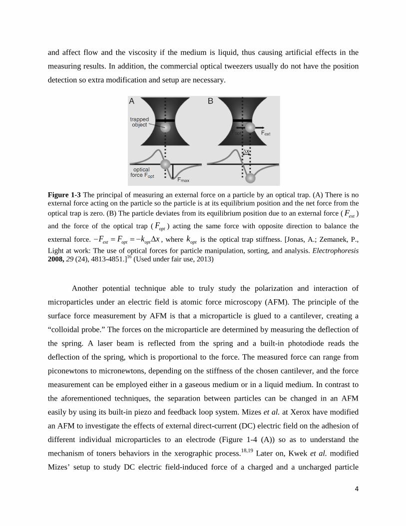
Figure 1-3 The principal of measuring an external force on a particle by an optical trap. (A)
There is no external force acting on the particle so the particle is at its equilibrium position and
the net force from the optical trap is zero. (B) The particle deviates from its equilibrium position
due to an external force ( extF ) and the force of the optical trap ( optF ) acting the same force with
opposite direction to balance the external force. ext optF F k x− = = − ∆ , where optk is the optical
trap stiffness. (Reprinted from Ref. 16) .......................................................................................... 4
Figure 1-4 (A) Scheme of Mizes’ setup to study the electrostatic adhesion of microparticles
(reprinted from Ref. 18); (B) The modified setup based on Mizes’ setup to study DC electric
field-induced force of a microparticle between the parallel condenser electrodes (reprinted from
Ref. 20). .......................................................................................................................................... 5
Figure 2-1 Real and imaginary parts of complex permittivity and dielectric dispersion of a
heterogeneous lossy dielectric versus the applied frequency (Modified from Ref. 28) ................. 8
Figure 3-1 Schematic of the polarization of an uncharged particle under an electric field when (a)
the polarizability of the particle is greater than the suspending medium or (b) the polariability of
the particle is less than the suspending medium. (Reprinted from Ref. 27) ................................. 12
Figure 3-2 Numerically calculated electric field lines of four different situations: (a) the particle
is more polarizable than the medium and the field is uniform; (b) the particle is less polarizable
than the medium and the field is uniform; (c) the particle is more polarizable than the medium
and the field is non-uniform; (d) the particle is less polarizable than the medium and the field is
non-uniform. (Reprinted from Ref. 27) ........................................................................................ 12
Figure 3-3 Two dimensional electric field distributions around two identical particles align with
an axis connecting the centers of the particles parallel to the direction of an applied uniform
electric field: (a) particles are more polarizable than the medium so positive DEP occurs; (b)

xii
particles are less polarizable than the medium so negative DEP occurs. (Reprinted from Ref. 27)
....................................................................................................................................................... 14
Figure 3-4 Two dimensional electric field distributions around two identical particles align with
an axis connecting the centers of the particles perpendicular to the direction of an applied
uniform electric field: (a) particles are more polarizable than the medium so positive DEP occurs;
(b) particles are less polarizable than the medium so negative DEP occurs. (Reprinted from Ref.
27) ................................................................................................................................................. 15
Figure 3-5 The two charges in a dipole experiences different forces in magnitudes of a non-
uniform electric field. (Reprinted from Ref. 7) ............................................................................. 16
Figure 3-6 A dielectric particle with radius R and permittivity suspending in a fluid with
permittivity under a uniform electric field in z direction. (Reprinted from Ref. 7) .................. 17
Figure 3-7 Calculated DEP spectra of homogeneous dielectric spheres with ohmic loss but no
dielectric loss when (a) 0/ 2.5mε ε = , 0/ 10.0pε ε = , 84 10mσ−= × S/m, 810pσ −= S/m and
5R = µm, and (b) 0/ 10.0mε ε = , 0/ 1.0pε ε = , 810 /m S mσ −= , 710pσ −= S/m and 5R = µm.
(Modified from Ref. 7) ................................................................................................................. 23
Figure 3-8 (a) Schematic of the replacement of multilayered spherical particle with an equivalent
homogeneous sphere of the same radius but with the effective permittivity. (Reprinted from Ref.
7) (b) The DEP spectrum of the tow-layered spherical particle. The solid line represents Re[ ]K
and the dot line represents Im[ ]K . (Reprinted from Ref. 27) ...................................................... 25
Figure 3-9 (a) Electric field-induced interaction between two identical spheres i and j in an
electric field. ijr is the separation between the centers of the particles and ijθ is the angle between
the line-of-center and the electric field. (b) Calculated square of the effective relative
polarizability 2effβ versus dimensionless frequency in terms of the Maxwell-Wagner relaxation
time: (I) 10d cβ β= ; (II) 0.1d cβ β= . (Modified from Ref. 5) ...................................................... 27
Figure 3-10 An equivalent circuit for formulating the interparticle force of a one-diemensional
particle chain in AC-DC fields. (Reprinted from Ref. 31) ........................................................... 29
Figure 4-1 (a) The behavior of the cantilever in an AM mode (Modified from ref. 43) (b) Scheme
of an AFM setup in the AM mode. (Reprinted from ref. 41) ....................................................... 35

xiii
Figure 4-2 (a) The behavior of the cantilever in an FM mode. (Adapted from Ref. 43) (b)
Scheme of an AFM setup in the FM mode. (Reprinted from Ref. 41) ......................................... 36
Figure 4-3 Scheme of the operation principle of a KPFM. (Reprinted from ref. 44) ................... 39
Figure 4-4 On the left, a typical raw data diagram of the deflection of the cantilever (i.e., the
deflection of the laser beam for the catnielver) vs. the piezo position (i.e., the displacement of the
piezo) from a force measurement by AFM is shown. On the right, the scheme of the behaviors of
a cantilever with respect to a flat sample in a force measurement is illustrated. (Modified from
ref. 34) ........................................................................................................................................... 40
Figure 4-5 The procedure for converting a cantilever deflection vs. piezo displacement curve to a
force vs. distance curve. (Reprinted from Ref. 46) ....................................................................... 41
Figure 5-1 Schematic of apparatus. The sphere attached to the cantilever is referred to as the “top
sphere” whereas the sphere attached to the scanner is referred to as the “bottom sphere ............ 43
Figure 5-2 Effect of air-flow on deflection of AFM cantilever in glove bag. Plot shows
deflection of cantilever as a function of time with no air flow (top) and with air flow (bottom). 44
Figure 5-3 (a) Raw data showing deflection–piezo position with the field on or off. (b) Net Force
as a function of separation after the zero field data has been subtracted. ..................................... 46
Figure 6-1 The three different systems considered here (a) Two spheres system: The field-
induced force between two BaTiO3 glass microspheres was measured. Note that the measured
force in this system contains the contribution from the cantilever. (b) Cantilever-only system.
This is used to determine the effect of the field on the cantilever. (c) Cantilever-bottom sphere
system. This is used to determine the interaction between the cantilever and bottom sphere. The
dash circles represent the locations of the spheres in the two spheres system, which means the
separations between the cantilever and the bottom electrode in these three systems are the same.
....................................................................................................................................................... 50
Figure 6-2 (a) Comparison of the force under an electric field (at 60 V and 5 kHz) to the force
without applying electric filed from the cantilever-only system. The separation here is the
distance between the cantilever and the bottom electrode. (b) The comparisons of three
separation-dependent forces from three different systems at 60 V and 5 kHz. Note the separation
here is the distance between two spheres in the two spheres system. For the cantilever-only
system, the separation should be “separation + 60 μm”; for the cantilever-bottom system, it
should be “separation + 30 μm.” ................................................................................................... 51

xiv
Figure 6-3 Time series data of the deflection signal of the two spheres system when the applied
voltage is 60 V and the applied frequency is: (a) 10 kHz; (c) 26 kHz; (e) 27 kHz and the
corresponding FFT spectra (b), (d) and (f) respectively. The resonant frequency of the colloidal
probe is 53 kHz. ............................................................................................................................ 52
Figure 6-4 Time series data of the deflection signal of the two spheres system when the applied
voltage is 60 V and the applied frequency is: (a) 40 kHz; (c) 50 kHz; (e) 55 kHz; (g) 82 kHz and
the corresponding FFT spectra (b), (d), (f) and (h) respectively. The resonant frequency of the
colloidal probe is 53.0 kHz. .......................................................................................................... 53
Figure 6-5 The comparison of the magnitude of different peaks that response at 0 (i.e., static
component), 0f , 2 f and rf at different applied frequencies ( 0f ). ............................................. 54
Figure 6-6 The scheme of the configuration of the cantilever and electrodes, where g is the gap
between the cantilever and bottom electrode, G is the gap between the two electrodes, 'g is the
gap between the cantilever and the bottom electrode, z is the displacement of the cantilever, V
is the applied voltage, V1 is the voltage between the cantilever and bottom electrode, and V2 is
the voltage between the cantilever and top electrode. Note that V=V1+V2. The bottom electrode
was totally fixed. Although the top electrode was fixed at one end, it still can be taken as “totally
fixed” due to its large mass inertia. The cantilever was only fixed at one end. ............................ 55
Figure 6-7 Time series data of the deflection signal of the cantilever-only system when the
applied voltage is 60 V and the applied frequency is: (a) 75 kHz; (c) 80 kHz; (e) 82 kHz and the
corresponding FFT spectra (b), (d) and (f) respectively. The resonant frequency of the cantilever
is 164 kHz. .................................................................................................................................... 56
Figure 6-8 The comparison of the magnitude of different peaks that response at 0 (i.e., static
component), 0f and 02 f at different applied frequencies ( 0f ). ................................................... 57
Figure 6-9 The correlation between the applied electric field strength and the amplitude of the
peak at (a) the applied frequency 0f and (b) twice the applied frequency 02 f in the two spheres
system. .......................................................................................................................................... 58
Figure 6-10 The variation of the AC electric field-induced force with the separation between two
BaTiO3 glass microspheres at the applied voltage: (a) 30 V and (b) 60 V when the applied
frequency is around half the resonant frequency of the colloidal probe (i.e., 53 kHz). ................ 59

xv
Figure 6-11 The comparison of the magnitude of the colloidal probe vibration responses at twice
the applied frequency when the applied voltages are 30, 60 and 100 V. ...................................... 60
Figure 6-12 The variation of the deflection signal at the separation between the two BaTiO3 glass
microspheres ranged from (a) 0.90 to 1.00 µm; (b) 0.40 to 0.50 µm as the applied voltage is 60 V
and the applied frequency is 5 kHz and at the separation ranged from 0.90 to 1.00 µm when the
applied voltage is 100 V and the applied frequency is (c) 5 kHz; (d) 100 kHz. ........................... 61
Figure 6-13 The variation of the deflection signal with the separation between the two BaTiO3
glass microspheres at different applied voltages and frequencies: (a) 60 V, 5 kHz; (b) the
enlargement of the bouncing point of (a); (c) 100 V, 5 kHz; (d) 100 V, 100 kHz. ...................... 62
Figure 6-14 (a) The variation of the AC electric field-induced forces with the separation between
two BaTiO3 glass microspheres at different frequencies when the applied voltage is 60 V. (b)
The variation of the AC electric field-induced forces with frequencies at different applied
voltages when the separation between the two dielectric microspheres is 2.5 μm. ...................... 64
Figure 6-15 The variations electric field-induced force between two dielectric microspheres with
time when the applied voltage is (a) 60 V and (b) 120 V and the distance between the two
spheres is around 6 μm. The electric fields were applied after AFM started to record the data for
about 5 seconds. (c) The variation of normalized DC electric field-induced force with time at
difference applied voltages. .......................................................................................................... 66
Figure 6-16 Relationship of the electric field-induced forces between two BaTiO3 glass
microspheres with the square of the applied electric field at different separation as the applied
frequency is 100 kHz. ................................................................................................................... 67
Figure 6-17 (a) Comparison of the measured electric field-induced force with calculated results
from different models and the fit to a simple power law, 20/ b
cF E a x −= ⋅ , where a and b are
constants and b=0.5671. (b) The enlargement of (a) at small separation. .................................... 68
Figure 6-18 The linearity between ln F and ln cx . ...................................................................... 69
Figure 6-19 The variation of the AC electric field-induced adhesion with different applied
frequencies when the applied voltages are 100, 60 and 30, respectively. The dash lines represent
the average values of each set of data. .......................................................................................... 70
Figure 6-20 (a) Adhesion force with field on and off. The solid spots means field off and the
hollow spot means field on. (b) Correlation between the number of time of two spheres contact
and the adhesion force. ................................................................................................................. 71
xvi
Figure 6-21 Relationship between the electric field-induced adhesion force and the square of the
applied electric field strength under a DC and an AC electric field, where the frequency of the
AC field is 100 kHz. The dash lines are the linear fitting results. ................................................ 72

xvii
List of Tables Table 3-1 Different behaviors and forces for a particle in different conditions ........................... 11
Table 3-2 Mathematical expressions for the moment, electric potential, and z-directed force due
to the linear multipoles, or any axisymmetric charge distribution. (Reprinted from Ref. 7) ........ 19
Table 3-3 Summary of some mathematical expressions based on the effective moment method
for some specific cases.7 ............................................................................................................... 22
Table 6-1 Brief summary of the bouncing point at different applied voltages and frequencies. .. 63

1
Chapter 1 – Introduction
1.1 Literature Review and Thesis Motivation The forces between microparticles induced by an external electric field play an important
role in many areas, such as powder contamination in the semiconductor industry, xerography,1
electric field stabilized fluidized bed,2 electrostatic separation,3 electrorheological fluids4,5 and
micro- and nano-electromechanical systems (MEMS and NEMS).6 Although there are numerous
studies on surface and interfacial phenomena of particles, not many are related to the effects of
external electric fields, and even fewer studies on the closely spaced microparticles under an
electric field where the point-dipole approximation may fail. One of the reasons for the lack of
study in this area is the limits of the measurement techniques. So far, the measurement
techniques for studying the electric-field induced interactions and/or forces are mainly
dielectrophoretic (DEP) levitation, optical tweezers, atomic force microscopy (AFM) and some
home-built apparatus.
Dielectrophoretic (DEP) levitation is principally used to study the field-induced effective
dipole moment and Calusius-Mossotti function of single microparticles and microparticle chains,
which both are proportional to the electric field-induced force (i.e, dielectrophoretic force, which
will be introduced in detail in Chapter 3).7,8 The principle of the DEP levitation is to adjust the
applied voltage and frequency so that the electric field induced force would be equal to the
buoyant force with opposite direction, levitating the particle(s).7 The reduced equation of motion
for the levitated particle(s) in an equilibrium condition can be expressed as
3 21 0 1 00 4 Re[ ( )]bm g R K Vπ ε ω α α= − + (1.1)
where bm is the buoyant mass of particle(s), g is gravitational acceleration, R is it the radius of
the levitated particles, 1ε is dielectric constant of the medium where the particles suspend, ( )K ω
is the Calusius-Mossotti function and it is a complex number if the applied field is an AC field,
Re[ ( )]K ω means the real part of the Calusius-Mossotti function, 0α and 1α are the coefficients
depending on the geometry and spacing of the electrodes, and 0V is the applied voltage.7 Figure
1-1 depicts a typical DEP levitation system. However, the density of individual microparticles
used for calculating the buoyant mass is hard to determine due to their small size.7 Furthermore,

2
the DEP levitator cannot control the separation between the particles; it is thus not able to study
the correlation of the particle chains and the separation between/among the particles.
Figure 1-1 Schematic of a digital active feedback controlled DEP levitation system [Tombs, T. N.; Jones, T. B., DIGITAL DIELECTROPHORETIC LEVITATION. Review of Scientific Instruments 1991, 62 (4), 1072-1077.]8 (Used under fair use, 2013)
Wang et al. have developed a home-built apparatus to control the separation between the
particles and which is able to directly measure the electric field-induced forces between two
particles in both liquid and gaseous media as shown in Figure 1-2.9,10,11 Nevertheless, the size of
the particle they used is around 6 mm and the smallest of the separation between the particles is
0.01 mm, which cannot truly show the field-induced interaction between closely spaced
microparticles. Rankin et al. have modified a rheometer for the application of an electric field so
as to study the electric field polarization mechanisms of electrorheological behavior.12 The
parameter they measured is the yield stress of a solution of BaTiO3 with diameters in the range
53-90 µm and silicone oil under an electric field. However, the modified rheometer only can be
used to study the collective behavior of microparticles in fluids, not the behavior of individual
particles. Besides, the separation between the particles cannot be controlled by this technique.

3
Therefore, it is very difficult to extract the fundamental force-separation data from their
experiment.
Figure 1-2 Schematic of an apparatus for measuring electric field-induced force between two particles with a computer-controlled elevator to adjust the separation between the particles [Wang, Z. Y.; Peng, Z.; Lu, K. Q.; Wen, W. J., Experimental investigation for field-induced interaction force of two spheres. Applied Physics Letters 2003, 82 (11), 1796-1798.]9 (Used under fair use, 2013)
Several research groups13,14,15 have adapted optical tweezers to truly investigate the
interaction between individual microparticles under an electric field. Optical tweezers basically
use a laser beam to manipulate particles ranged in diameter from ~20 nm to several
micrometers.16,17 Because of the dual nature of light, the mechanism of manipulating particles by
a laser beam can be explained from the particle and wave viewpoints respectively. From the
aspect of the particle nature of light, when light irradiates particles, light would be scattered and
absorbed by the particles, depending on the refractive indexes of the particles and the medium.
The change in direction and magnitude of photon momentum causes an equal and opposite
change in the particle momentum, applying a force to the particle.16 The displacement of the
particles from their own equilibrium position is proportional to the force of the optical trap so the
trap can be taken as a linear spring and used to measure external forces on the particles, as shown
in Figure 1-3. The “spring constant” of the optical trap (i.e., optical trap stiffness) depends on the
optical gradient (i.e., how tightly the laser is focused), the laser power, the size and optical
properties of the trapped particles and the optical properties of the medium.16,17 However, the
magnitude of the force that optical tweezers can measure is ranged from femtonewtons to
piconewtons.17 Thus, it is not suitable to use optical tweezers to study strong electric field-
induced force. Also, local heating due to the high power laser beam may damage the particles
4
and affect flow and the viscosity if the medium is liquid, thus causing artificial effects in the
measuring results. In addition, the commercial optical tweezers usually do not have the position
detection so extra modification and setup are necessary.
Figure 1-3 The principal of measuring an external force on a particle by an optical trap. (A) There is no external force acting on the particle so the particle is at its equilibrium position and the net force from the optical trap is zero. (B) The particle deviates from its equilibrium position due to an external force ( extF )
and the force of the optical trap ( optF ) acting the same force with opposite direction to balance the
external force. ext opt optF F k x− = = − ∆ , where optk is the optical trap stiffness. [Jonas, A.; Zemanek, P., Light at work: The use of optical forces for particle manipulation, sorting, and analysis. Electrophoresis 2008, 29 (24), 4813-4851.]16 (Used under fair use, 2013)
Another potential technique able to truly study the polarization and interaction of
microparticles under an electric field is atomic force microscopy (AFM). The principle of the
surface force measurement by AFM is that a microparticle is glued to a cantilever, creating a
“colloidal probe.” The forces on the microparticle are determined by measuring the deflection of
the spring. A laser beam is reflected from the spring and a built-in photodiode reads the
deflection of the spring, which is proportional to the force. The measured force can range from
piconewtons to micronewtons, depending on the stiffness of the chosen cantilever, and the force
measurement can be employed either in a gaseous medium or in a liquid medium. In contrast to
the aforementioned techniques, the separation between particles can be changed in an AFM
easily by using its built-in piezo and feedback loop system. Mizes et al. at Xerox have modified
an AFM to investigate the effects of external direct-current (DC) electric field on the adhesion of
different individual microparticles to an electrode (Figure 1-4 (A)) so as to understand the
mechanism of toners behaviors in the xerographic process.18,19 Later on, Kwek et al. modified
Mizes’ setup to study DC electric field-induced force of a charged and a uncharged particle

5
respectively by varying the position of the microparticles between the parallel condenser
electrodes as shown in Figure 1-4 (B).20 All the measurements by Mizes et al. and Kwek et al.
were in ambient environment, which are strongly influenced by water adsorbed on the particle,
and were measured in the presence of a DC field, not an alternating-current (AC) field, which
make them strongly influenced by surface conductivity.21,22,23
(A) (B)
Figure 1-4 (A) Scheme of Mizes’ setup to study the electrostatic adhesion of microparticles [Mizes, H. A., ADHESION OF SMALL PARTICLES IN ELECTRIC-FIELDS. Journal of Adhesion Science and Technology 1994, 8 (8), 937-951.]18 (Used under fair use, 2013); (B) The modified setup based on Mizes’ setup to study DC electric field-induced force of a microparticle between the parallel condenser electrodes. [Kwek, J. W.; Vakarelski, I. U.; Ng, W. K.; Heng, J. Y. Y.; Tan, R. B. H., Novel parallel plate condenser for single particle electrostatic force measurements in atomic force microscope. Colloids and Surfaces a-Physicochemical and Engineering Aspects 2011, 385 (1-3), 206-212.]20 (Used under fair use, 2013)
Based on the above introduction, we believe that AFM enables to measure the field-
induced force between closely spaced microparticles varying with the separation between the
particles, thus helping to clarify the real phenomena and mechanisms that the studies by other
measurement techniques have simplified and/or overlooked.
1.2 Objectives and Outline of This Thesis The objective of this work is to study polarization forces between particles, particularly at
small separations (less than the particle diameter). To maximize the polarization, we used two
BaTiO3 glass microparticles. To minimize the effects of surface conductivity, we used a low
6
humidity environment. We used an AFM to measure the forces, and built a pair of parallel
electrodes in an AFM similar to Mizes’ apparatus. In contrast to Mizes’ work, we study both AC
and DC field-induced forces. The response to a DC field is dominated by surface conductivity
whereas the response to an AC field is dominated by polarization. We have three fundament
variables: (1) the frequency of the applied field, which explores the frequency dependence of
polarization; (2) the applied field strength, which helps to determine the mechanism of the force
(as described later, a polarization force should be proportional to the square of the field) and (3)
the separation between the particles, which also helps us to understand the perturbation of the
applied field by a second particle. The use of high frequency fields induced high frequency
forces, which required us to synchronize two different data acquisition methods with different
sample rates. Through these experiments, we hope that this study will improve the understanding
of the polarization and interaction between microparticles under an electric field, facilitating the
development of applications involving field induced forces. This thesis will show that the
electrical field-induced forces are much, much larger than the traditionally studied van der Waals
and double-layer surface forces and thus offer a greater ability to control microparticles.
In the following chapters of this thesis, we will first introduce basic definitions of solid
dielectric materials and some basic dielectric theory in Chapter 2, including the mechanisms of
electric polarization and the frequency response of dielectrics under an AC electric field, which
are required for the analysis of electric field-induced interactions and forces between dielectrics.
Then the theories of polarization and interaction of particles under an electric field will be
explained in Chapter 3. Chapter 4 will describe the principles of AFM and the technique of force
measurement by AFM in detail. Chapter 5 will describe the home-built apparatus for this work,
sample preparation, some experimental methods and methods for data analysis in detail. The
experimental and theoretical results accompanying with discussion will be shown in Chapter 6.
7
Chapter 2 – Electric Polarization and Relaxation of Solid Dielectrics Ideal dielectrics do not permit the passage of any particles, including electrons (i.e., the
conductivity is zero) so they are also referred to ideal insulators and taken as capacitors
electrically.24,25 Nevertheless, real dielectrics always contain some free electrons but far fewer
than conductors so that real dielectrics have finite conductivity. The differences between real
dielectrics and semiconductor are that semiconductors have higher conductivity and the
dominate charge carriers in semiconductor are attributed to thermal excitation (i.e., electron-hole
generation) but in dielectrics are due to other sources, such as charge injection and optical
excitation.24 When the dielectrics have finite conductivity, the dielectrics can be said “lossy” and
are electrically equivalent to an ideal lossless capacitor in parallel with a resistor.26 The
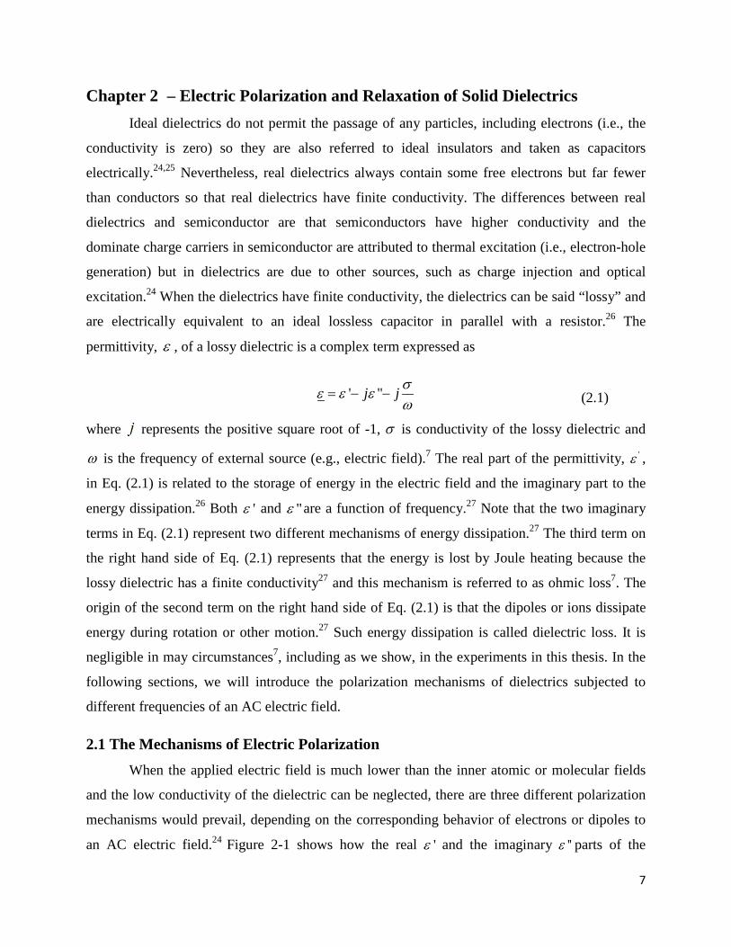
permittivity, ε , of a lossy dielectric is a complex term expressed as
' "j jσε ε εω
= − − (2.1)
where represents the positive square root of -1, σ is conductivity of the lossy dielectric and
ω is the frequency of external source (e.g., electric field).7 The real part of the permittivity, 'ε ,
in Eq. (2.1) is related to the storage of energy in the electric field and the imaginary part to the
energy dissipation.26 Both 'ε and "ε are a function of frequency.27 Note that the two imaginary
terms in Eq. (2.1) represent two different mechanisms of energy dissipation.27 The third term on
the right hand side of Eq. (2.1) represents that the energy is lost by Joule heating because the
lossy dielectric has a finite conductivity27 and this mechanism is referred to as ohmic loss7. The
origin of the second term on the right hand side of Eq. (2.1) is that the dipoles or ions dissipate
energy during rotation or other motion.27 Such energy dissipation is called dielectric loss. It is
negligible in may circumstances7, including as we show, in the experiments in this thesis. In the
following sections, we will introduce the polarization mechanisms of dielectrics subjected to
different frequencies of an AC electric field.
2.1 The Mechanisms of Electric Polarization When the applied electric field is much lower than the inner atomic or molecular fields
and the low conductivity of the dielectric can be neglected, there are three different polarization
mechanisms would prevail, depending on the corresponding behavior of electrons or dipoles to
an AC electric field.24 Figure 2-1 shows how the real 'ε and the imaginary ''ε parts of the

8
complex permittivity vary with different frequency due to loss of a series of response
mechanisms.28
Figure 2-1 Real and imaginary parts of complex permittivity and dielectric dispersion of a heterogeneous lossy dielectric versus the applied frequency [Hao, T.; Kawai, A.; Ikazaki, F., Mechanism of the electrorheological effect: Evidence from the conductive, dielectric, and surface characteristics of water-free electrorheological fluids. Langmuir 1998, 14 (5), 1256-1262.]28 (used under fair use, 2013)
The response mechanisms are:
1. Electronic polarization: At UV frequencies (~1015 to ~1016 Hz), the electron clouds of atoms
or molecules are displaced with respect to the inner positive nucleus. This polarization exists in
any kind of dielectrics.
2. Atomic or ionic polarization (vibrational polarization): The ions or atoms of a polyatomic
molecule are moved relative to each other due to the external electric field, causing a change in
dipole moment.
3. Orientational polarization (or Debye relaxation): This polarization only happens in polar
dielectric. The electric field would drive the permanent dipoles to align toward the direction of
the electric field.
~1015~109~103

9
There is a fourth type polarization that occurs when the low conductivity of the dielectric
cannot be neglected (or the applied field is high enough): the migration of charge carriers. When
the migration of charge carriers is impeded at the interface between two unlike dielectrics and/or
grain boundaries of the dielectric, then an accumulation of charge occurs at the interface.24 This
is so-called “interfacial or space charge polarization”24 and is also referred to as “Maxwell-
Wagner interfacial polarization” since the theory was developed by James Clerk Maxwell and
later on refined by K.W. Wagner29. This polarization exists in amorphous or polycrystalline
solids or materials consisting of trapped charges.24 The movement of charge to the surface takes
time, so this mechanism only operates at low frequencies or in a DC electric field. Jones has
investigated this time-dependent phenomenon by deriving the time-dependent effective dipole
moment of a homogeneous ohmic dielectric sphere with permittivity 2ε , conductivity 2σ , and
radius R in a ohmic dielectric fluid with permittivity 1ε and conductivity 1σ (Eq. (2.2)).7
3 32 1 2 11 0 1 0
2 1 2 1
( ) 4 [1 exp( / )] 4 exp( / )2 2eff MW MWp t R E t R E tσ σ ε επε τ πε τ
σ σ ε ε − −
= − − + − + + (2.2)
where 2 1
2 1
22MW
ε ετσ σ
+=
+ is Maxwell-Wagner charge relaxation time associated with the charge
accumulation at the surface of the sphere. When MWt τ<< (i.e., high frequency), the first term on
the right hand side of Eq. (2.2) would be negligible and the effective moment is dominate by the
permittivities, meaning no charge accumulation at the surface of the sphere. However, when
MWt τ>> (i.e., low frequency), the first term on the right hand side of Eq. (2.2) dominates if
charge accumulation can occur at the surface. Since the field-induced force is proportional to the
effective dipole moment, we can expect that the field-induced force would have a similar
frequency response. The relationship between the field-induced force and the effective moment
would be introduced in detail in Chapter 3.

10
Chapter 3 – Electromechanics of Particles Every material has its own special electrical properties, thus having different responses,
such as polarization and field-induced forces, to an external electric field. In Chapter 2, different
electric polarizations and the corresponding mechanisms have been introduced. In this chapter,
we focus on the forces that the particles with diameter range from 1 to 1000 µm experience
through the action of an external electric field and/or an induced-field by other nearby polarized
particles. The forces can be categorized based on the types of the applied electric field and the
particles’ surroundings (e.g., high conductivity electrolyte or air) as electrophoresis (EP),
dielectrophoresis (DEP), electrorotation (ROT), electroosmosis (EO), electrohydrodynamics
(EHD), and so forth.27 Herein we mainly cover DEP since in our study it is the main mechanism
and the others do not occur or can be ignored.
First the fundamentals and some equations of the DEP are introduced. Then two
analytical models of electric field-induced forces between two identical particles developed from
different points of view are reviewed. We will use these models to interpret our experimental
observations in Chapter 6.
3.1 General Overview of Dielectrophoresis (DEP) DEP refers to the translation motion of an uncharged dielectric and/or conductive particle
caused by polarization effects in a non-uniform electric field.7,29 EP is the movement of a
charged particle resulted from the Coulomb force between the particle and an electric field.27
Different from EP, DEP is basically attributed to the interaction of an electric field with the
electric field-induced dipole moments.27 In addition, DEP can occur not only in a DC electric
field but also in an AC electric field as long as the electric field is non-uniform, which can be
from the directly applied a non-uniform external electric field and/or indirectly generated by
other nearby polarized particles7,27 as is the case in the work described in this thesis. Although a
uniform electric field can also induce dipole moments in an uncharged particle, the vector sum of
these dipoles is zero, causing no motion of the particle. On the other hand, EP can only occur in a
DC electric field since the direction of the EP force depends on the polarity of the electric field
and an AC field would cause the charged particle to oscillate around an axis but not move from
that average point over time; that is, the EP force is averaged to zero in an AC field.29 Therefore,

11
we can conclude different behaviors and forces of a particle under an electric field as follows
(Table 3-1).
Table 3-1 Different behaviors and forces for a particle in different conditions
Uncharged Particle Charged particle
DC field
Both DEP and EP occur in a non-uniform filed. EP occurs due to the accumulated charges at the interface of the particle. In a uniform field, only EP occurs.
Both DEP and EP occur in a non-uniform field and only EP occurs in a uniform filed.
AC field
Only DEP occurs if the field is non-uniform. Otherwise, neither DEP nor EP will occurs. The particle will oscillate.
Only DEP occurs if the field is non-uniform. Otherwise, neither DEP nor EP will occurs. The particle will oscillate.
One of interesting features of DEP is that the polarized particle is not always attracted to
the region of the stronger electric field. It is opposite under certain conditions instead. When the
particle is more polarizable than its environment (medium), more induced charge separation
takes place in the particle than in the medium, causing higher charge density inside the interface
than outside and the effective dipole across the particle is in the same direction as the electric
field, as shown in Figure 3-1 (a). If the applied field is non-uniform, then the particle is attracted
and to the high-field region, which is termed positive DEP. This is the case in the experiments
described in this thesis, where we have a high dielectric particle in air, and the particle is near
another particle. On the contrary, if the particle is less polarizable than the medium, the effective
dipole across the particle in the opposite direction to the electric field (Figure 3-1 (b)). If the
applied field is non-uniform, the particle would be repelled from the high-field region. In other
words, the particle is attracted to the low-field region in a non-uniform electric field when the
polarizability of the particle is less than the medium. The phenomenon is termed negative DEP.

12
Figure 3-1 Schematic of the polarization of an uncharged particle under an electric field when (a) the polarizability of the particle is greater than the suspending medium or (b) the polariability of the particle is less than the suspending medium. [Morgan, H.; Green, N. G., AC Electrokinetics: colloids and nanoparticles. Research Studies Press: Philadelphia, PA, 2003.]27 (Used under fair use, 2013)
Figure 3-2 Numerically calculated electric field lines of four different situations: (a) the particle is more polarizable than the medium and the field is uniform; (b) the particle is less polarizable than the medium and the field is uniform; (c) the particle is more polarizable than the medium and the field is non-uniform; (d) the particle is less polarizable than the medium and the field is non-uniform. [Morgan, H.; Green, N. G., AC Electrokinetics: colloids and nanoparticles. Research Studies Press: Philadelphia, PA, 2003.]27 (Used under fair use, 2013)

13
Figure 3-2 shows the electric field lines of the above situations. Note that the electric field line
on both sides of the particle is symmetric when the electric field is uniform no matter whose
polarizability is greater (Figure 3-2 (a) and (b)), meaning the net DEP force exerted on the
particle is zero in a uniform field. Further, as the polarizability of the particle greater than the
medium, the electric field lines inside the particle is near zero and the lines outside it would bend
to and/or be perpendicular to the surface of the particle, just like a metal sphere in an electric
field (Figure 3-2 (a) and (c)). By contrast, the particle would act as an insulator as its
polarizability less than the medium. The outside electric field lines would bend around the
particle and the density of the inside lines is similar to those outside. If the particle and the
medium have the same polarizability, there is no effective dipole across the particle and no DEP
occurs.
In addition to the electrical properties of the particle and the medium and the non-
uniformity and strength of the electric field, the frequency of the applied field can control the
direction and the magnitude of the DEP force as well. At low frequencies, the accumulation of
the free charge at the interface between the particle and the medium (i.e., a Maxwell-Wagner
interfacial polarization as mentioned in Chapter 2) dominates the DEP force. The amount of the
accumulated charge on either side of the interface depends on the impedance of these materials
and the frequency of the applied field. In other words, the conductivitiesI 30, of the particle and the
medium dominate the DEP force. At high frequencies, the permittivities of the particle and the
medium dominate the DEP force since the charge within the particle is not able to respond to the
high frequency field. At the intermediate frequency range, the transition from positive DEP to
negative DEP or from negative DEP to positive DEP takes place. This is referred to as dielectric
dispersion.7,27,29 The detail of frequency-dependent DEP would be reviewed in Section 3.2.2.
So far we have discussed DEP on a single particle. But particle-particle interactions are
often important in applications, and are the subject of this thesis. Here two cases of particle-
particle interactions are stated and their calculated electric field distributions are shown in Figure
3-3 and Figure 3-4, respectively. The first case is that the axis connects the centers of two
identical particles (i.e., line-of-centers) parallel to the direction of an applied uniform electric
IThe more accurate terminology should be “admittance”, not “conductivity.” The admittance in an AC electric field is analogous to the electrical conductance in a DC field.30 The admittance is complex but usually the real part, which is the electrical conductance, is considered in most discussions. Further, the electrical conductance is proportional to the electrical conductivity so “conductivity” is used in most literatures and models.

14
field, as shown in Figure 3-3. The darker part in the figures means lower field strength and the
lighter part means higher field strength. In Figure 3-3 (a), the particle are more polarizable than
the medium so they experience positive DEP. Note that the field strength between the particles is
higher than those of the other sides of the particles and the particles would move to high-field
region so they would move to each other. On the other hand, the particles are less polarizable
than the medium in Figure 3-3 (b) so they experience negative DEP. Interestingly the particle
move to each other as well since the field strength between the particles is lower than those of
the other sides of the particles. As a result, two identical particles would “attract” to each other
when their line-of-centers parallels to the direction of the applied electric field no matter whether
Figure 3-3 Two dimensional electric field distributions around two identical particles align with an axis connecting the centers of the particles parallel to the direction of an applied uniform electric field: (a) particles are more polarizable than the medium so positive DEP occurs; (b) particles are less polarizable than the medium so negative DEP occurs. [Morgan, H.; Green, N. G., AC Electrokinetics: colloids and nanoparticles. Research Studies Press: Philadelphia, PA, 2003.]27 (Used under fair use, 2013)
the polarizability of the particles is greater or smaller than the medium. The second case is
similar to the first one but the direction of the electric field is perpendicular to the line-of-centers
of the particles (Figure 3-4). Contrary to the first case, two identical particles would “repel” each
other and move to the region with their favorable field strength (e.g., particles experiencing
positive DEP move to high-filed regions) to reach a stable state (i.e., like the arrangement in the
first case) no matter whether their polarizability is greater or smaller than the medium. In
conclusion, for identical particles under an electric field, the direction of force is determined by
the angle between the electric field and the line-of-centers of the particles, not the polarizability.

15
Figure 3-4 Two dimensional electric field distributions around two identical particles align with an axis connecting the centers of the particles perpendicular to the direction of an applied uniform electric field: (a) particles are more polarizable than the medium so positive DEP occurs; (b) particles are less polarizable than the medium so negative DEP occurs. [Morgan, H.; Green, N. G., AC Electrokinetics: colloids and nanoparticles. Research Studies Press: Philadelphia, PA, 2003.]27 (Used under fair use, 2013)
We have briefly introduced some features of the DEP from a phenomenological
perspective. The following will introduce some related equations of DEP in the electromagnetic
and mathematical point of view.
3.2 Analysis of DEP by Effective Moment Method
3.2.1 General Overview of Calculation of DEP force by Effective Moment Method
To derive the equation of the DEP force, first we need to consider a force on an
infinitesimal dipole in a non-uniform electric field since the origin of the DEP is the interaction
of a non-uniform electric field with the induced field-dipole. As shown in Figure 3-5, a dipole
consists of two charges of equal magnitudes and opposite signs separated by a vector distance d
in an electric field E
. Assume that the charges are stationary or with negligible velocities and
accelerations so the movement of the charges does not change the electric field much and thus is
negligible, which is referred to as a quasi-electrostatic system.7

16
Figure 3-5 The two charges in a dipole experiences different forces in magnitudes of a non-uniform electric field. [Jones, T. B., Electromechanics of Particles. Cambridge University Press: New York City, NY, 1995.]7 (Used under fair use, 2013)
Thus, the net force on the dipole is
( ) ( )F qE r d qE r= + −
(3.1)
where r
is the position of –q. If d
is smaller than the characteristic dimension of the electric
field nonuniformity (i.e., the electric field is nearly uniform across the dipole), the electric field
can be expanded around r
by a vector Taylor series, given by
( ) ( ) ( ) ...E r d E r d E r+ = + ⋅∇ +
(3.2)
Substituting Eq. (3.2) into Eq. (3.1) gives
( ) ( ) ( ) ... ( )F qE r qd E r qE r qd E r= + ⋅∇ − + ≈ ⋅∇
(3.3)
where the higher order terms (i.e., d2, d3, and so on) is neglected. For a finite dipole,
dipoleF p E= ⋅∇
(3.4)
Eq. (3.4), referred to as dielectrophoretic approximation, can be applied to any physical dipoles,
such as a polar molecule or a polarized particle with finite size.7 Note that this approximation
demonstrates that the force on a dipole is zero in a uniform electric field, corresponding to the
previous statement.
However, higher order terms in Eq. (3.3) should be taken into consideration when the
characteristic dimension of the electric field nonuniformity is comparable to the dimension of the
object we concern, such as the case of closely spaced particles where the dimension of the
nonuniformity of the local electric field induced by the particles is comparable to the particle size.
Herein the effective moment method is introduced to approximate the p
in Eq. (3.4) more
17
accurately for the calculation of the DEP force of a particle. The idea of this method is to
hypothesize that the DEP force of a particle can be expressed by the effective moments effp
derived from solving the induced electrostatic field due to the particle.7 The reasons for this
choice are that its ease of implementation and validity in many cases where is hard to employ the
derivations based on the Maxwell stress tensor.7
Here the derivation of the effective moment in the simplest case is reviewed first since
this can derive the effective moments of other more general cases simply by adjusting some
parameters to the corresponding situations. Subsequently, the general expression of effective
moment and the limitation of this method are stated.
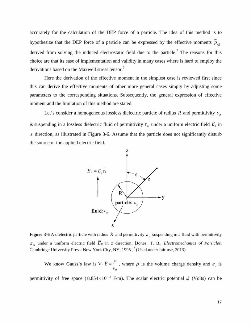
Let’s consider a homogeneous lossless dielectric particle of radius R and permittivity pε
is suspending in a lossless dielectric fluid of permittivity mε under a uniform electric field 0E in
z direction, as illustrated in Figure 3-6. Assume that the particle does not significantly disturb
the source of the applied electric field.
Figure 3-6 A dielectric particle with radius R and permittivity pε suspending in a fluid with permittivity
mε under a uniform electric field 0E
in z direction. [Jones, T. B., Electromechanics of Particles. Cambridge University Press: New York City, NY, 1995.]7 (Used under fair use, 2013)
We know Gauss’s law is 0
E ρε
∇ ⋅ =
, where ρ is the volume charge density and 0ε is
permittivity of free space ( 128.854 10−× F/m). The scalar electric potential φ (Volts) can be

18
related to the vector electric field by E φ= −∇
. Thus, we can get 2
0
ρφε
∇ = − , which is referred
to as Poisson’s equation. As the charge density is zero, we obtain 2 0φ∇ = , which is termed
Laplace’s equation. Due to the conservation of an electrostatic field26 and no existence of free
charge (i.e., both the particle and the medium are lossless) in this case, the curl and the
divergence of the electric field are zero. As a result, the electric potential satisfies Laplace’s
equation everywhere for this case. Assume the dipole moment is the dominate contribution
compared with other multipoles, which can be ignored. Hence the general solutions for Laplace’s
equation are assumed7
0 2
cos( , ) cos ,mAr E r r R
rθφ θ θ= − + > (3.5)
( , ) cos ,p r Br r Rφ θ θ= − < (3.6)
where mφ and pφ are the potential within the fluid and the sphere, respectively and A and B are
unknown constants. The first term on the right hand side of Eq. (3.5) represent the applied
electric field and the second term represents the induced dipole due to the particle.
To specify the solutions, we need to find out the boundary conditions at the particle
surface (i.e., r R= ). The first boundary condition is the continuity of the normal electric field
components across the particle-fluid boundary, which can be rewritten as
( , ) ( , )m pr R r Rφ θ φ θ= = = (3.7)
The second boundary condition is the continuity of the normal components of the electric flux
density (or electric displacement) D
(Cm-2) across the boundary. D
is defined as D Eε=
. Thus
the second boundary condition can be written as
( , ) ( , )m rm p rpE r R E r Rε θ ε θ= = = (3.8)
where mrmE
rφ∂
= −∂
and prpE
rφ∂
= −∂
are the normal electric field components in the fluid and the
particle, respectively. Substituting Eq. (3.5) and (3.6) into Eq. (3.7) and (3.8), we obtain

19
302
p m
p m
A R Eε εε ε
−=
+ and 0
32m
p m
B Eεε ε
=+
(3.9)
Based on the concept of the effective moment method, the effective dipole moment of the
polarized particle in this case can be taken as an equivalent, free-charge, point dipole offering the
same dipolar electric potential dipoleφ II
, which is
2
cos4eff
dipolem
prθ
φπε
= (3.10)
Table 3-2 Mathematical expressions for the moment, electric potential, and z-directed force due to the linear multipoles, or any axisymmetric charge distribution. [Jones, T. B., Electromechanics of Particles. Cambridge University Press: New York City, NY, 1995.]7 (Used under fair use, 2013)
Comparing the second term on the right hand side of Eq. (3.5) with Eq. (3.10), we can get
IIThe expressions of the electric potential by linear multipoles are summarized in Table 3-2 and the detailed derivations by Legendre polynomials can be found in Ref. 7 and 26. Here we directly use the derived results.

20
3 30 04 4 4
2p m
eff m m mp m
p A R E KR Eε ε
πε πε πεε ε
−= = =
+ (3.11)
( , )2
p mp p
p m
Kε ε
ε εε ε
−=
+ (3.12)
K is known as the Clausius-Mossotti function, representing the strength of the effective
polarization of a spherical particle.7 Note that K can point out the relative direction of the
applied electric field and the effective dipole moment. As 0K > (i.e., p mε ε> ), the dipole and
applied electric field point in the same direction; however, as 0K < (i.e., p mε ε< ), the dipole
points toward the opposite direction to the electric field, corresponding to the statement in
section 3.1.1.
Finally, substituting Eq. (3.11) into Eq. (3.4), dielectric approximation gives
3 202 ( )
2p m
DEP mp m
F R Eε ε
πεε ε
−= ∇
+
(3.13)
However, Eq. (3.13) only can be applied to the case we specified. Table 3-3 summarizes the
effective moments, Calusius-Mossotti function, electric potentials, and forces for more general
cases. The detailed derivations of these expressions can be found in Ref. 7. Note that these
mathematical formulas look very similar to Eq. (3.11) and (3.13) and they all can be derived by
the equations in Table 3-2. As for lossy materials, the permittivities should be in the complex
form, which is represented by underlining ε , so does Calusius-Mossotti function. In addition,
the lossy properties of materials are significant under an AC electric field; thus the DEP
behaviors of lossy materials under an AC field are discussed, so do that in Table 3-2. Thus the
concept of phasor, a representation of a complex number in terms of a complex exponential by
Euler formula, is introduced to rewrite time-varying parameters, such as electric field and
potential for the connivance of calculation. For example, 0 0 0cos Re[ exp( )]z zE E te E j t eω ω= =
and 0 0 exp( ) zE E j t eω=
is the vector phasor expression of a sinusoidal AC electric field. Only
the real part, which is denoted Re[…], is meaningful. That is why the real part of the force is
considered in Table 3-3. Furthermore, the force under an AC electric field consists of a constant
(average) term and a time-varying term. Since the motion due to the time-varying term is usually

21
damped heavily by the viscosity of the suspension medium for the particle size range from 1 to
1000 μm7, Table 3-3 only pays attention on the time-average term, which is designated <…>.
However, the medium we used in our study is air so the time-varying term should be studied as
well. We will discuss the time-varying term in detail in Chapter 6.
Note that the effective moment method is not rigorous for lossy dielectrics since potential
energy arguments are not legitimate.7 Even so, the effective moment method is still very useful
because in most circumstance, dielectric loss is negligible and there is no much difficulty to
adjust the method when dielectric loss cannot be neglected.
3.2.2 Frequency-Dependent DEP
Let’s now consider the case of a homogenous particle with ohmic loss but no dielectric
loss suspended in a dielectric medium under an electric field. Eq. (T3.4) and (T3.10) point out

22
Table 3-3 Summary of some mathematical expressions based on the effective moment method for some specific cases.7
Only consider dipole moment Consider both dipole and other mutipoles
Lossless dielectric homogeneous sphere
3
04eff mp KR Eπε= (3.11)
( , )2
p mp p
p m
Kε ε
ε εε ε
−=
+ (3.12)
2
cos4eff
dipolem
prθ
φπε
= (3.10)
3 2
02 ( )2
p mDEP m
p m
F R Eε ε
πεε ε
−= ∇
+
(3.11)
( ) 2 1 1
( )1
4( 1)!
n n nn m z
n
K R Epn z
πε + −
−
∂=
− ∂ (T3.5)
( )
( 1)p mn
p m
Kn n
ε εε ε
−=
+ + (T3.6)
2
( 1)!4
nz
n n nm
E n qz
φπε ζ +
∂ += − =
∂ (T3.7)
ζ : the distance between the electric field source and the center of the particle
( )
2( ) 2 1 1
1
( )!
2!( 1)!
nnn z
n n zn n
n n nm z
zn
EpF q d E en z
K R E en n z z
πε + −
−
∂= ⋅∇ =
∂
∂∂= − ∂ ∂
(T3.8)
Ohmic lossy dielectric homogeneous sphere
304 meff
p KR Eπε=
(T3.1)
0 1( )2 2 1
p m p m
p m p m MW
jKj
σ σε ε ωτωε ε σ σ ωτ
−− += = + + +
(T3.2)
22
p mMW
p m
ε ετ
σ σ+
=+
, 0p m
p m
ε ετ
σ σ−
=−
(T3.3)
* 3 21( ) Re[ ] 2 Re[ ( )]
2 m rmseffF t p E R K Eπε ω= ⋅∇ = ∇
(T3.4)
( )
( 1)n p m
p m
Kn n
ε εε ε
−=
+ + (T3.9)
212 1
( ) ,( )1
2 Re[ ]!( 1)!
nnn z rmsn m
z n
ERF Kn n z zπε −+
−
∂∂= − ∂ ∂ (T3.10)

23
that Re[ ]K is the factor to determine the frequency dependence of the time-averaged DEP force.
To study the frequency-dependent DEP, we can merely focus on Re[ ]K . From Eq. (T3.2), we
can get
2 2 2
3( )Re[ ]
2 ( 2 ) (1 )p m m p p m
p m MW p m MW
Kε ε ε σ ε σε ε τ σ σ ω τ
− −= +
+ + + (3.14)
where MWτ depicts the decay of a dipolar distribution of free charge at the surface of the particle.7
Applying two frequency-limitations to the ( )K ω gives
0
lim Re[ ]2MW
p m
p m
Kωτ
σ σσ σ→
−=
+ (3.15)
lim Re[ ]2MW
p m
p m
Kωτ
ε εε ε→∞
−=
+ (3.16)
Eq. (3.15) and (3.16) confirm two different DEP behaviors at low and high frequencies,
respectively, that is, the conductivities of the sphere and medium govern the low-frequency DEP
Figure 3-7 Calculated DEP spectra of homogeneous dielectric spheres with ohmic loss but no dielectric loss when (a) 0/ 2.5mε ε = , 0/ 10.0pε ε = , 84 10mσ
−= × S/m, 810pσ −= S/m and 5R = µm, and (b)
0/ 10.0mε ε = , 0/ 1.0pε ε = , 810 /m S mσ −= , 710pσ −= S/m and 5R = µm. [Jones, T. B., Electromechanics of Particles. Cambridge University Press: New York City, NY, 1995.]7 (Used under fair use, 2013)
p m
m p
σ σ
ε ε
<
<
m p
p m
σ σ
ε ε
<
<

24
behavior and the permittivities of the sphere and medium governs the high-frequency DEP
behavior. Figure 3-7 shows the variation of Re[ ]K versus the applied electric field frequencies
in different conditions. Note that at a certain frequency, Re[ ]K becomes zero and there is no
DEPF . This frequency is so-called crossover frequency since the force has opposite sign on either
side of this frequency.29 For the work in this thesis, the medium is always air, so the dielectric
constant and conductivity of the particles is always greater than the medium.
3.2.3 Models for Layered Spherical Particles
So far, we have only concerned homogeneous spheres. As for heterogeneous spheres, we
briefly introduce the particle with shell structure here. The principle of the model for layered
spherical particles is to replace a layered spherical particle with an equivalent homogeneous
particle of the same radius but with the effective permittivity, as shown in Figure 3-8 (a), so that
the mathematical expressions for a homogenous sphere above are still valid for the layered
sphere as long as the permittivity of the homogeneous sphere is replaced by the effective
permittivity of the layered sphere.7 So the general expression of the effective permittivity is
3 1
' 1
3 1
1
22
2
N N
N NN N
N N
N N
a
a
ε εε ε
ε εε εε ε
+
+
+
+
−+ + = − − +
(3.17)
where 1/N Na R R += and N+1 indicates the most inner layer so N represents the layer shells the
most inner layer. Eq. (3.17) can be applied repeatedly for multilayer structure. As shown in
Figure 3-8 (a), we can use 3ε and 4ε to calculate the effective permittivity '3ε first and then use
'3ε and 2ε to calculate '
2ε . In addition, Eq. (3.17) is for a sphere with ohmic loss but no dielectric
loss and Maxwell-Wagner relaxation happens for each interface. For a lossless sphere, we can
just replace the complex form of permittivities by the real form of permittivies. In fact, the
derivation of Eq. (3.17) is similar to that in section 3.2.1 so it is valid only for a uniform or
nearly uniform electric field since only the dipole is concerned. For a layered sphere with ohmic
loss but no dielectric loss in a nonuniform field, higher mutilpolar terms should be concerned,
which gives

25
( )2 1
'2 ( )2 1
( 1)( )nn
n nn
a n Ka nK
ε+
+
+ = −
(3.18)
where ( )nK is defined as Eq.(T3.9). Similarly, for a lossless sphere, we can just replace ( )nK by ( )nK defined as Eq. (T3.6).
Figure 3-8 (a) Schematic of the replacement of multilayered spherical particle with an equivalent homogeneous sphere of the same radius but with the effective permittivity. [Jones, T. B., Electromechanics of Particles. Cambridge University Press: New York City, NY, 1995.]7 (Used under fair use, 2013) (b) The DEP spectrum of the tow-layered spherical particle. The solid line represents Re[ ]K and the dot line represents Im[ ]K . [Morgan, H.; Green, N. G., AC Electrokinetics: colloids and nanoparticles. Research Studies Press: Philadelphia, PA, 2003.]27 (Used under fair use, 2013)
It is noteworthy that Eq. (3.17) is the same as Maxwell’s classic mixture formula for the
effective permittivity of a mixture consisting of noninteracting spherical particles in a medium
with very low volume fraction (i.e., 1ϕ << )7,27, which is usually written as
(a)
(b)
Re[
K] a
nd Im
[K]

26
1 22
12
p m
p mmix m
p m
p m
ε εϕ
ε εε ε
ε εϕ
ε ε
−+ + =
− − +
(3.19)
3.3Maxwell-Wagner Model of Interparticle Force in AC-DC Electric Fields Maxwell-Wagner Model is the simplest model to simulate the electric-field interparticle
force resulting from both the perimittivites and condcutivities of identical dielectric spheres with
ohmic loss and an ohmic lossy dielectric medium by combining the effective moment method
with the point-dipole approximation.5 The derivation of this model starts at solving Laplace’s
equation of an isolated dielectric sphere with ohmic loss in a uniform AC electric field and
assuming the induced dipole moment is the dominate contribution of the particle polarization,
like the derivation in section 3.2.1. Combining the concept of the point-dipole approximation, the
time-averaged force on a sphere i at the origin due to another identical sphere j at ( , )ij ijr θ as,
shown in Figure 3-9 (a), can be expressed
6
2 2 24
12( , ) ( ) [(3cos 1) (sin 2 ) ]mij ij ij eff rms ij r ij
RF r E e er θπεθ β ω θ θ= − +
(3.20)
where 0 / 2rmsE E= , and the effective relative polarizability effβ is
2 2 2
22
( )1 ( )
c d mweff
mw
β β ωτβωτ
+=
+ (3.21)
where
2p m
dp m
ε εβ
ε ε−
=+
, 2
p mc
p m
σ σβ
σ σ−
=+
(3.22)
Interestingly, if we apply two frequency limits to Eq. (3.21), we can find similar results to Eq. (3.15) and (3.16). That is,
2 2lim ( )
MWeff dωτ
β ω β→∞
= (3.23)
2 2
0lim ( )MW
eff cωτβ ω β
→= (3.24)

27
which also demonstrate that the conductivities of particles and medium govern the field-induced
force in a DC and/or low-frequency AC electric fields and the permittivities of particles and
medium govern the force in a high-frequency AC fields. Likewise, to see the frequency
dependence of the electric field-induced interparticle force, we merely focus on the variation of 2 ( )effβ ω with frequency, which is plotted in Figure 3-9 (b).
Figure 3-9 (a) Electric field-induced interaction between two identical spheres i and j in an electric
field. ijr is the separation between the centers of the particles and ijθ is the angle between the line-of-
center and the electric field. (b) Calculated square of the effective relative polarizability 2effβ versus
dimensionless frequency in terms of the Maxwell-Wagner relaxation time: (I) 10d cβ β= ; (II)
0.1d cβ β= . [Parthasarathy, M.; Klingenberg, D. J., Electrorheology: Mechanisms and models. Materials Science & Engineering R-Reports 1996, 17 (2), 57-103.]5 (Used under fair use, 2013)
3.4 Equivalent Circuit Model of Interparticle Force in AC-DC Electric Fields Different from the electromagnetic point of view above, Colver has employed the
concept of equivalent circuits to develop an interparticle force model of for electric field
stabilized gas-fluidized beds31, as illustrated in Figure 3-10. The resistance-capacitance
components in this model result in two time constants: self-particle charge relaxation time pτ
and particle-particle relaxation time bτ for transient decay of charge within a particle and
between two particles, respectively. To formulate the model, Colver came up some assumptions
as follows.
0E
(a) (b)
(I)
(II)ijr

28
(1) The concerned spherical powders are in a cubic packing.
(2) Particles are semi-insulating with a small but finite surface electrical conductivity (i.e.,
ohmic loss) and finite contact resistance at point of contact.
(3) Self-particle charge decay is no influenced by neighboring particles and can be evaluated
using single-particle relaxation theory. The single particle charge relaxation time is
0' ( 2 )4
pp
s
dε ετ
σ+
= (3.25)
where d is the particle diameter and sσ is the surface conductivity of the particle, which
can be given as
ln( )sp c
d dr
σπρ
= (3.26)
where pρ is the apparent (single) particle resistivity and cr is the particle contact radius.
(4) Particle-particle charge decay can be evaluated using continuum bed relaxation theory.
The bulk powder charge relaxation time is given as
'pb bτ ε ρ= (3.27)
where bρ is the apparent bulk powder resistivity and pε is the corresponding bulk
powder permittivity for bed voidage α , given as Eq. (3.28) and (3.29) respectively.
48 0.69 17.71 5.12 0.188(9.406 10 ) ( ) RHb E T d eρ − − −= × × (3.28)
where T is temperature (K) and RH is relative humidity (%) and this equation has been
tested up to 40% RH.
0 0
0
0
3 2 1
3 1
p p
p
p
ε εα
ε εεεε
αε
− −
=
+ −
(3.29)

29
(5) The equivalent circuit is comparable small to the wavelength of the applied signals so all
electrical signals travel through the circuit quickly, affecting every point in the circuit
simultaneously (i.e., lumped parameter circuit theory).30 Thus distributed capacitance and
resistance over the surface of a particle can be assumed having single values.
(6) Circuit components are linear, which means any steady-state output of the circuit (e.g.,
voltage and current) is also a sinusoidal signal with frequency f when the input signal is
a sinusoidal function with frequency f but they may not be in phase.
Figure 3-10 An equivalent circuit for formulating the interparticle force of a one-diemensional particle chain in AC-DC fields. [Colver, G. M., An interparticle force model for ac-dc electric fields in powders. Powder Technology 2000, 112 (1-2), 126-136.]31 (Used under fair use, 2013)
Clover also assumed the capacitors in the circuit are simple parallel plate capacitors.
Therefore the contact capacitance cC at the interface between the particles and the self-particle
capacitance pC are given as
'2
0 01
cc
c c
A rC Kx x
ε ε π= = ,
'2
2p
p
rC K
dε π
= (3.30)
where cx is the separation distance between the particles, cA is the effective capacitance area, 'r
is the radius of cA and the constants 1K and 2K account for effective capacitance area,
distributed capacitance, curvature of particles, and the average contact separation distance.

30
For the application of the model to both AC and DC fields, a sinusoidal applied field
( ) exp( )V t V j tω= is assumed. Based on Kirchhoff’s law, we can obtain the differential equation
depicting the AC (or DC as 0ω → ) voltage drop across the contact capacitance cV
[1 ] j tc c cp
b pc
dV V V j edt
ωωττ τ
+ = + AC or DC ( 0ω → ) (3.31)
where the time constants are defined as
1 [ ] [ ]1/ 1/
p cb p c p c
p c p c
pc cpc p c
p c p c p c
R RC C C C
R R R R
RR RR R R R R R
τ
τ τ τ
= + = + + +
= = ++ + +
(3.32)
where cR is the particle contact resistance, pR is the single particle resistance
[ ]pc p p c p p cR C C R Cτ τ= + = + , p p pR Cτ = and c c cR Cτ = is the particle contact relaxation time.
Solving Eq. (3.32) gives
2
0 1 22
1 ( )exp exp ( )
1 ( )pb
cb pc b
tV A V j tτ ωτ ω δ δ
τ τ τ ω +
= − + × + − + (3.33)
where 1δ and 2δ are defined as 1tan 1/ bδ ωτ= and 2tan 1/ pδ ωτ= , respectively. On the right
hand side of Eq. (3.33), the first term is the transient response and the second term is the steady-
periodic response. The interparticle force can be taken as the force acting on the plates of the
contact capacitor. Since the transient term would diminish over time, we can ignore it and also
the phase angle (i.e., 1 2 0tω δ δ+ − = ), obtaining the peak force per unit area
222max 0 0 0
2
220
02
1 ( )2 2 1 ( )
1 ( )2 1 ( )
pc b
c b pc c
p b
b pc c
F E VxA
d Ex
τ ωε ε ττ ω τ
τ ωε ττ ω τ
+= =
+
+=
+
, AC/DC (3.34)
where '2cA rπ= and the separation distance between the particles is assumed smaller than the
diameter of the particle so the applied voltage can be rewritten in terms of the electric field

31
strength in the far-field. Further, the time-averaged interparticle force per unit area can be
expressed
22
0 max2
1 ( )2 1 ( ) 2
avg p brms
c cb pc c
F Fd ExA A
τ ωε ττ ω τ
+= =
+ , AC (3.35)
where 0 / 2rmsE E= is the rms value for the applied sinusoidal field.
To cover both AC and DC fields, Colver further combined DC field interparticle force
equation Eq. (3.36) with Eq. (3.34), giving more general AC-DC interparticle force equation Eq.
(3.37).
2 20dc bkF d E Eβ βδπε −= DC (3.36)
2
2 2max 0 2
1 ( )1 ( )
pbk
b
F d E Eγ
β βτ ωδπε
τ ω−
+=
+ (3.37)
where δ , β , and γ are constants and bkE is the electric breakdown strengthIII
Although Colver’s model is based on the concept of the equivalent circuit, some features
of his model correspond or similar to some conclusions from the effective moment method and
Maxwell-Wagner model, which are summarized as follows.
between the
spheres.
(1) The mathematical expressions of the electric field-induced force from these three models
all show the force is proportional to the square of the rms value of the applied electric
field.
(2) Colver’s model also shows that the force would either increase of decrease with
frequency. Colver mentioned that it is the relative magnitude of pτ and bτ that
determines the trend of the force with the frequency. Note that Eq. (3.25) Eq. (3.27) can
be used to calculate these two time constants based on the assumptions (3) and (4). In
addition, the permittivity and conductivity of the particles would always greater than the
IIIElectric (or dielectric) breakdown strength is the maximum electric field strength that an insulating material can withstand without any current leakage.25 Once the electric field strength larger than this value, the insulating material would not be insulating anymore, but conductive.

32
medium in Colver’s model since he derived his model for air medium. Thus we can infer
that the trend of the force depends on the relative magnitude of the permittivity and
surface conductivity of the particles and the resistivity and the permittivity of bulk
powder in Colver’s model.
(3) Besides pτ and bτ , Colver also pointed out that /p cC C governs the magnitude of the
forces at large values of bτ ω and /c pR R governs the force at small values of bτ ω . Note
that 0/ ( / )( / )p c c pC C x d ε ε= as 1 2K K K= = for simplification. Then in other words, we
can interpret that the force is governed by the perimitivities of the particles and air at high
frequency and by the conductivities of the particles and the air at low frequency when the
separation distance between the two particles are fixed.
We will use these models to interpret our experimental results in Chapter 6.

33
Chapter 4 – Atomic Force Microscopy (AFM) and the Technique of Force
Measurements AFM is well-known for its ability to image surface topography at the micro- and/or
nanoscale. However, what AFM can really do is far more than this by a well-designed
experiment, the choice of operation modes, instrumental modification, and/or methods of data
acquisition.32 Besides imaging, AFM has used in the measurements of different surface forces
(e.g., van der Waal and adhesion forces)33,34 and nanoscale dielectric constant,35 the quantitative
study of elastic and viscoelastic properties and tribology, including friction, wear and
lubrication,36,37 picogram mass sensors,38 nanoscale fabrication,39 and so on, shown the
versatility of this instrument. In this charter, we will focus on the technique of force
measurement, which is used in the work. But in the beginning, we will briefly introduce basic
concepts and modes of AFM before talking about the measurement of forces.
4.1 Basic Concepts and Modes of AFM There are mainly five parts in AFM: 1) cantilevers and the attached tips, 2) laser beam 3)
photodiode (i.e., photo dectactor), 4) piezoelectric positioner (usually shorten to piezo), and 5) a
feedback loop, as shown in Figure 4-1. Before the measurement, the laser beam is focused at the
end of the cantilever and deflects to the photodiode. When the tip on the cantilever feels or
senses some forces between itself and the sample, the cantilever would start to bend, thus
changing the position of the deflected laser beam on the photodiode. At this moment, the signal
detected by the photodiode would be fed into a DC feedback amplifier in the feedback loop,
comparing with the set point determined by the operator. The resulting difference (i.e., error
signal) is sent to a proportional–integral–differential (PID) controller to make the piezo adjust
the separation between the cantilever and the sample, keeping the deflection of the laser beam
equal to the set point. The adjustment of the piezo generates the image of the sample surface.40
Note that the stiffness of the cantilever would affect how small the force can be reflected to the
photodiode. The softer the cantilever is, the smaller the force can be detected, which can be
explained by Hooke’s law and the stiffness of the cantilever is also called the spring constant of
the cantilever. In addition, the apex radius and the geometry of the tip would affect how small
the indentation and the convexity at the surface of the sample can be probed by the tip. Thus, the
combination of the cantilever and tip would determine the resolution of an AFM image since the

34
sensitivity and the quality of the photodioe, piezo, and the feedback loop for commercial AFMs
are quite similar nowadays.
The operation of AFM can be divided into several modes based on whether the cantilever
oscillates or not and the types of the set point. Here, a static mode – contact mode and two
dynamic modes – amplitude modulation (AM) and frequency modulation (FM) modes are
introduced. Besides those three basic modes, we will also introduce a Kelvin probe force
microscopy (KPFM), which is related to this work.
Contact mode
The features of the contact mode are that the cantilever does not oscillate, the tip would
directly touch the sample while imaging and can be used in both ambient conditions and liquids
due to its simplicity. The set point of this mode is the deflection of laser beam on the photodiode.
Although this mode is mostly used, it would cause the damage either of the sample or of the tip,
depending on which one is harder, thus distorting the features of generated image and not
suitable for imaging soft materials, such as biomaterials and polymers.40
Amplitude-Modulation (AM) Mode
The principle of the AM mode is shown in Figure 4-1. First the cantilever is mechanically
excited at or near its free resonant frequency (i.e., the resonant frequency without the effect of
tip-sample interaction). When the tip approaches the sample and starts to sense the force, the
deflection of the laser beam from the cantilever would change and is detected by the photodiode.
The detected signal is sent to a lock-in amplifier to get the information of the amplitude and
phase of the oscillating cantilever for comparing with the set point, a chosen amplitude of the
oscillation, usually is 70-80% of the free amplitude (the amplitude at the free resonant
frequency). As state before, the calculated error signal from the DC feedback amplifier is fed
into the PID controller to control the piezo, keeping the detected signal from the photodiode (or
the detected amplitude) is the same as the set point.41 The adjustment of the piezo here is the
topography of the sample surface as well. In addition, the difference between the detected phase
and the phase from the driving force for exciting the cantilever can give the map of the material
properties of the sample, such as soft or hard.42 The AFM mode is usually used in ambient

35
conditions and liquids, but not in the ultra high vacuum (UHV), which would slow down the
speed of imaging.41-43
(a)
(b)
Figure 4-1 (a) The behavior of the cantilever in an AM mode [Melitz, W.; Shen, J.; Kummel, A. C.; Lee, S., Kelvin probe force microscopy and its application. Surface Science Reports 2011, 66 (1), 1-27.]43 (Used under fair use, 2013) (b) Scheme of an AFM setup in the AM mode. [Schirmeisen, A.; Anczykowski, B.; Hölscher, H.; Fuchs, H., Dynamic Modes of Atomic Force Microscopy. In Nanotribology and nanomechanics. Volume 1, Measurement techniques and nanomechanics, Bhushan, B., Ed. Springer: Berlin ; Heidelberg ; New York 2011; pp 307-353.]41 (Used under fair use, 2013)
Conventionally, the AM-mode is also called the tapping mode since the cantilever is
oscillating at or near its free resonant frequency, causing the tip touch the sample shortly but

36
frequently.40 However, the AM-mode can be used in a non-contact mode as well,42 which is
confusing; thus, it is better to name the modes based on the type of the set point and the
operation principle of the feedback loop.
Frequency-Modulation (FM) Mode
Similar to the AM-mode, the cantilever is excited at its free resonant frequency in the FM
mode as well. Nevertheless the set point of the FM mode is the free resonant frequency of the
(a)
(b)
Figure 4-2 (a) The behavior of the cantilever in an FM mode. [Melitz, W.; Shen, J.; Kummel, A. C.; Lee, S., Kelvin probe force microscopy and its application. Surface Science Reports 2011, 66 (1), 1-27.]43 (Used under fair use, 2013) (b) Scheme of an AFM setup in the FM mode. [Schirmeisen, A.; Anczykowski, B.; Hölscher, H.; Fuchs, H., Dynamic Modes of Atomic Force Microscopy. In Nanotribology and nanomechanics. Volume 1, Measurement techniques and nanomechanics, Bhushan, B., Ed. Springer: Berlin ; Heidelberg ; New York 2011; pp 307-353.]41 (Used under fair use, 2013)
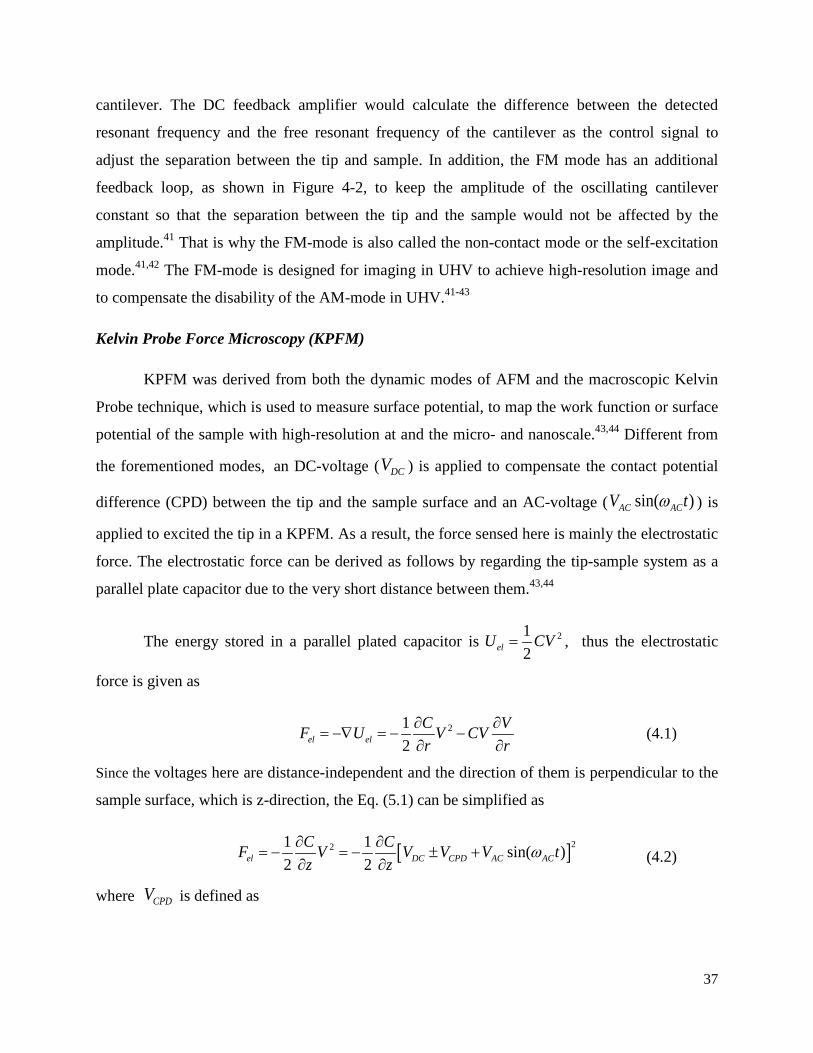
37
cantilever. The DC feedback amplifier would calculate the difference between the detected
resonant frequency and the free resonant frequency of the cantilever as the control signal to
adjust the separation between the tip and sample. In addition, the FM mode has an additional
feedback loop, as shown in Figure 4-2, to keep the amplitude of the oscillating cantilever
constant so that the separation between the tip and the sample would not be affected by the
amplitude.41 That is why the FM-mode is also called the non-contact mode or the self-excitation
mode.41,42 The FM-mode is designed for imaging in UHV to achieve high-resolution image and
to compensate the disability of the AM-mode in UHV.41-43
Kelvin Probe Force Microscopy (KPFM)
KPFM was derived from both the dynamic modes of AFM and the macroscopic Kelvin
Probe technique, which is used to measure surface potential, to map the work function or surface
potential of the sample with high-resolution at and the micro- and nanoscale.43,44 Different from
the forementioned modes, an DC-voltage ( DCV ) is applied to compensate the contact potential
difference (CPD) between the tip and the sample surface and an AC-voltage ( sin( )AC ACV tω ) is
applied to excited the tip in a KPFM. As a result, the force sensed here is mainly the electrostatic
force. The electrostatic force can be derived as follows by regarding the tip-sample system as a
parallel plate capacitor due to the very short distance between them.43,44
The energy stored in a parallel plated capacitor is 212elU CV= , thus the electrostatic
force is given as
212el el
C VF U V CVr r
∂ ∂= −∇ = − −
∂ ∂ (4.1)
Since the voltages here are distance-independent and the direction of them is perpendicular to the
sample surface, which is z-direction, the Eq. (5.1) can be simplified as
[ ]221 1 sin( )2 2el DC CPD AC AC
C CF V V V V tz z
ω∂ ∂= − = − ± +
∂ ∂ (4.2)
where CPDV is defined as

38
tip smapleCPDV
e eφ φφ −∆
= =− −
(4.3)
where tipφ and smapleφ are work function of the tip and sample and e is the elementary charge.
Note that the sign of CPDV in Eq. (4.2) is determined by how DCV is applied to the sample or the
tip. Based on Eq. (4.3), we can calculate the work function of the sample by using the tip with a
known work function in KPFM. Further, elF can be divided into three forces by rearranging Eq.
(4.2).
2 21 1( )2 4DC DC CPD AC
CF V V Vz
∂ = − ± + ∂ (4.4)
( ) sin( )DC CPD AC ACCF V V V tzω ω∂
= − ±∂
(4.5)
2 cos(2 )4AC
ACVCF t
zω ω∂=∂
(4.6)
The operation principle of KPFM is based these three forces, DCF , Fω and 2F ω . We would also
use similar concepts to explain our results in chapter 8.
Since KPFM is based on the dynamic modes of AFM, it can be operated in either AM or
FM mode as well. The principles and feedback loops designs of AM- and FM-KPFM are show
in Figure 4-3. In AM-KPFM, the amplitude of the oscillating cantilever at ACω is taken as
control signal. Once the feedback loops get the signal of amplitude, it would adjust DCV to
minimize the difference between DCV and CPDV , thus nullifying Fω and the amplitude. The
adjustment of DCV is can be used to map the CPD of the sample.43 In FM-KPFM, the frequency
shift of the oscillation cantilever from ACω is the control signal instead. Similarly, the feedback
loops would adjust DCV to reduce the frequency shift and the adjustment of DCV can be converted
to the image of CPD since they possess the same magnitude but opposite sign.

39
Figure 4-3 Scheme of the operation principle of a KPFM. [Sadewasser, S., Experimental Technique and Working Modes. In Kelvin probe force microscopy: measuring and compensating electrostatic forces, Sadewasser, S.; Glatzel, T., Eds. Springer-Verlag Berlin Heidelberg: Heidelberg ; New York, 2012; pp 7-24.]44 (Used under fair use, 2013)
4.2 Technique of Force Measurement Both the contact mode and dynamic modes can be used in surface force measurement.33,41
Here we only introduce the fore measurement technique in contact mode since we use this mode
in this work.
The principle of surface force measurement by AFM, as shown in Figure 4-4, is different
from that of imaging. For imaging, the cantilever usually with a sharp tip would scan the sample
surface, which is controlled by a feedback loop. However, for force measurement, a microsphere
would be attach to the end of the cantilever, used as a tip/probe, and the cantilever or the sample,
depending on where the piezo is located, would approach and retract the sample surface as
illustrated in the right-hand side of Figure 4-4. The cantilever with a microsphere is so-called the
colloidal probe, which is developed to quantitatively measure the surface forces.33 The reasons
for using a microsphere rather than a sharp tip are as follows. First, the force between a colloidal
probe and sample is larger than that between a sharp tip, which usually only has a 5-10 nm
radius, and sample based on the Derjaguin approximation so the measurement can be more
accurate. The Derjaguin approximation is expressed as

40
1 2
1 2
( ) 2 ( )R RF D W DR R
π
≈ + (4.7)
where D is the distance between the two subjects (e.g., the colloid and the sample), 1R and 2R
the radii of the two subjects, respectively, and W the interaction free-energy.45 Second, more
quantitative analysis, such as calculating the surface energy by the Derijaguin approximation can
be proceeded since the geometry of the colloidal probe is known and it is easy to determine the
radius of a microsphere. Also, the surface roughness of a microsphere can be controlled and
examined easier than that of a small, sharp tip during manufacturing. Furthermore, we can
choose to use the microspheres made from different materials and/or coated with different
chemicals/materials, such as hydrophobic functional groups and gold to study surface forces in
different systems.33
Figure 4-4 On the left, a typical raw data diagram of the deflection of the cantilever (i.e., the deflection of the laser beam for the catnielver) vs. the piezo position (i.e., the displacement of the piezo) from a force measurement by AFM is shown. On the right, the scheme of the behaviors of a cantilever with respect to a flat sample in a force measurement is illustrated. [Ralston, J.; Larson, I.; Rutland, M. W.; Feiler, A. A.; Kleijn, M., Atomic force microscopy and direct surface force measurements - (IUPAC technical report). Pure and Applied Chemistry 2005, 77 (12), 2149-2170.]34 (Used under fair use, 2013)
A typical raw data curve from the force measurement by AFM is shown in the left-hand
side of Figure 4-4. There are five regions in this curve corresponding to different behaviors of
the cantilever which are illustrated on the right of Figure 4-4. In region I and V, the distance
between the probe and the sample is so large that the colloidal probe does not sense any force
and no bending of the cantilever. In region II, however, the distance is quite short; thus the
colloidal probe starts to sense some forces, either attractive (in Figure 4-4) or repulsive (in Figure
4-5), and the cantilever deflection is not flat anymore. In region III, the probe contacts the
V

41
sample and moves compliantly with the piezo. This linear region is called the constant
compliance region and reflects the optical sensitivity of the photodiode with respect to the
cantilever deflection, which is usually used to calibrate the cantilever deflection.34,46 In region IV,
the cantilever still contacts the sample but the piezo moves in an opposite direction. Once the
restoring force of the cantilever is large enough to pull off the cantilever itself from the sample
surface, the cantilever would jump back to the original position (i.e., region V) since the distance
between the colloidal probe and the sample is large and no surface force is sensed by the
colloidal probe.
Figure 4-5 The procedure for converting a cantilever deflection vs. piezo displacement curve to a force vs. distance curve. [Senden, T. J., Force microscopy and surface interactions. Current Opinion in Colloid & Interface Science 2001, 6 (2), 95-101.]46 (Used under fair use, 2013)

42
The standard procedure for converting the raw data to a force curve is illustrated in
Figure 4-5. Usually the cantilever deflection at large distance ( z in Figure 4-5) is assumed no
measured surface force and is used to define the zero of cantilever deflection signal. As
mentioned before, the slope of the constant compliance region (Ω ) is used to calibrate and
convert the cantilever deflection signal into units of distance. Then the calibrated and converted
deflection signal ( x ) would be multiplied by the calibrated spring constant of the cantilever with
the microsphere ( k ) to get the surface forces between the colloidal probe and the sample. The
separation or distance ( d ) between the colloidal probe and the surface is the relative movement
between the cantilever ( x ) and the piezo ( D ) and the contact position ( c ) is used to define the
zero separation.46 However, in this work, we modify this procedure since the electric field-
induced force is a very long-range force and we need to use the data collected under no electric
field to define the zero of the cantilever deflection signal. We will state our modify procedure in
Chapter 6 for details.

43
Chapter 5 – Experimental Section
5.1 AFM Setup This work was mainly performed with a CypherTM AFM (Asylum Research, Santa
Barbara, CA). To measure the FDEP between the two particles, we modified the AFM as shown in
Figure 5-1.
Figure 5-1 Schematic of apparatus. The sphere attached to the cantilever is referred to as the “top sphere” whereas the sphere attached to the scanner is referred to as the “bottom sphere
The electric field was created using two electrodes separated with a gap of 7.00 mm by a
rubber prop. Indium tin oxide (ITO) coated slides which are transparent but highly conductive
were chosen as the electrodes to allow the laser beam pass through the top electrode as shown in
Figure 5-1. The applied voltage was generated by a function generator (Mode1395 100 MHz
Synthesized Arbitrary Waveform Generator, Wavetek-Datron) and amplified 100× by a voltage
amplifier (Model 2100HF High Frequency High-Voltage Power Amplifier, Trek Inc.). The
voltage was varied from 60 to 220 V rms (root-mean-square). All voltages in this thesis are rms
values. The frequency was in the range from DC to 1 MHz.
To create a low humidity environment, the whole AFM was enclosed in a flexible glove
chamber (GLOVE BAG™ Inflatable Glove Chamber, Glas-Col LLC) supplied with dry air
Flexible Glove Chamber
E
ITO coated slide(transparent)
Dielectric spheres
Cantilever holder
Cantilever
LaserPhotodiode
x, y, z-scanner
Piezo
Dry Air
Humidity meter
Rubberprop
Functional Generator
Voltage Amplifier

44
continuously circulated. The RH can go down to less than 3% within around 1 to 2 hours but the
measurement was executed after about 8 hours of continuous flow to ensure the surface of the
microspheres and their surroundings are dry enough. During the measurement, dry air still
circulated to maintain the low humidity environment. The air flow did not significantly affect
AFM operation which has been examined by measuring the variation of the deflection of laser
beam with time (Figure 5-2). The RH and temperature in the chamber was monitored by a
humidity meter (THWD-3 Relative Humidity and Temperature Meter, Amprobe). All
measurements of field-induced interactions between two spheres were conducted at 2 ± 1 % RH
and 25 ± 3 °C.
Figure 5-2 Effect of air-flow on deflection of AFM cantilever in glove bag. Plot shows deflection of cantilever as a function of time with no air flow (top) and with air flow (bottom).
5.2 Sample Preparation A barium titanate (BaTiO3) glass microsphsere (MO-SCI Specialty Products, L.L.C.) was
attached to the end of a silicon rectangular shaped cantilever (tipless, NSC12/no backside metal
coating, MikroMasch) with heat-softening epoxy resin (Epikote 1004) by micromanipulators
under an optical microscope. The attachment was confirmed by an optical microscope. The
normal spring constants and resonant frequencies of the colloidal probes and cantilevers alone
were calibrated by the Hutter method47. The surface roughness of the microspheres on the
0 10 20 30 40 50 60 70 80 90 100
0.0
0.5
1.0
1.50 10 20 30 40 50 60 70 80 90 100
0.0
0.5
1.0
1.5
Varia
tion
of D
efle
ctio
n (n
m)
Time (s)
air flow
no air flow

45
cantilever was examined by inverse imaging with a TGT01 grating (NT-MDT). The
microspheres had a roughness less than 500 pm rms over the areas of 1 µm x 1 µm and 500 nm x
500 nm. For studying field-induced interactions between two spheres, the BaTiO3 glass spheres
were attached to a thin glass slide with epoxy resin by using micromanipulators. The sizes of the
microspheres used in this study verified by using the camera module of the AFM were
approximately 30 μm in diameter.
5.3 Alignment of Two Particles To investigate field-induced intershpereical interaction, the two microspheres were first
aligned manually using a video microscope that is part of the AFM, and then aligned more
accurately by imaging the bottom sphere with the top sphere. After imaging the sphere on the
glass slide on the bottom electrode by the colloidal probe, the commercial AFM software can
identify and control the relative position of the top and bottom spheres. Thus, we can align the
two microspheres and measure the force as a function of distance between the apexes of the
spheres via the software.34
5.4 Force Curve Collection and Analysis Since the electric field-induced force is a long range force, we modified the normal
procedure. In the normal method, the zero of force is determined from the force (deflection) at
large separation, where there is no surface force. When there is a very long range and slowly
varying force, it is difficult to know at what separation zero force occurs. In addition, there is a
complicating effect, the virtual deflection48, where the signal from the deflection varied slowly
with distance, even when there is no change in force.
Fortunately, the field-induced force can be conveniently turned on and off with a switch,
so we have established the zero force with the field turned off. Thus, for each condition (e.g., at
60 V and 5 kHz), two successive force curves, one with and one without an applied voltage, were
collected for around one second of each other. The measurement without an applied voltage was
used to determine “zero deflection” as in the normal method as shown in Figure 5-3 (a). The two
measurements (with and without the applied field) were each analyzed in the normal way, i.e. to
produce a force–separation plot, thereby ensuring that the two curves have the same zero of
separation, and were not shifted due to slight changes in temperature. The deflection signal in the

46
(a)
(b)
Figure 5-3 (a) Raw data showing deflection–piezo position with the field on or off. (b) Net Force as a function of separation after the zero field data has been subtracted.
absence of the field was then subtracted from the deflection signal in the field. An additional
effect of this subtraction is that all other contributions to the measured force are removed. We
have explicitly assumed that these other contributions are additive. These other contributions
include measurement artifacts due to variation in the laser signal with separation (virtual
-6 -5 -4 -3 -2 -1 0 1 2-200
0
200
400
600
800
1000
1200
1400
no E 60 V, 5 kHz
Piezo Position (µm)
Defle
ctio
n (n
m)
Jump-to-Contact
Piezo Position (µm)
Defle
ctio
n (n
m)
-2.5 -2.0 -1.5 -1.0 -0.5 0.0 0.5-100
-80
-60
-40
-20
0
20
40
0 1 2 3 4 5 6-400
-300
-200
-100
0
100
60 V, 5 kHz
Separation (µm)
Forc
e (n
N)
47
deflection and optical interference between reflections of light from the cantilever and sample)
and real forces, such as the van der Waals force. Thus, we assume that the van der Waals force is
not affected by the applied field. In practice, this is a small assumption because the van der
Waals force is very weak and short range (Figure 5-3 (a)) compared to the field-induced force,
and is usually only significant at separations where we are unable to measure data because of a
mechanical instability.
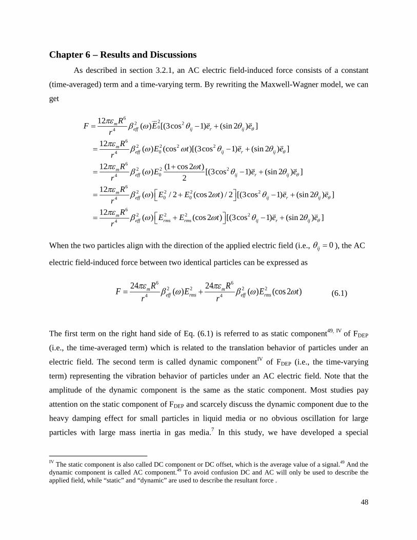
48
Chapter 6 – Results and Discussions As described in section 3.2.1, an AC electric field-induced force consists of a constant
(time-averaged) term and a time-varying term. By rewriting the Maxwell-Wagner model, we can
get
622 204
62 2 2 2
04
62 2 2
04
62 2
04
12 ( ) [(3cos 1) (sin 2 ) ]
12 ( ) (cos )[(3cos 1) (sin 2 ) ]
12 (1 cos 2 )( ) [(3cos 1) (sin 2 ) ]2
12 ( ) / 2
meff ij r ij
meff ij r ij
meff ij r ij
meff
RF E e er
R E t e er
R tE e er
R E Er
θ
θ
θ
πε β ω θ θ
πε β ω ω θ θ
πε ωβ ω θ θ
πε β ω
= − +
= − +
+= − +
= +
2 20
62 2 2 2
4
(cos 2 ) / 2 [(3cos 1) (sin 2 ) ]
12 ( ) (cos 2 ) [(3cos 1) (sin 2 ) ]
ij r ij
meff rms rms ij r ij
t e e
R E E t e er
θ
θ
ω θ θ
πε β ω ω θ θ
− +
= + − +
When the two particles align with the direction of the applied electric field (i.e., 0ijθ = ), the AC
electric field-induced force between two identical particles can be expressed as
6 6
2 2 2 24 4
24 24( ) ( ) (cos 2 )m meff rms eff rms
R RF E E tr rπε πε
β ω β ω ω= + (6.1)
The first term on the right hand side of Eq. (6.1) is referred to as static component49, IV
7
of FDEP
(i.e., the time-averaged term) which is related to the translation behavior of particles under an
electric field. The second term is called dynamic componentIV of FDEP (i.e., the time-varying
term) representing the vibration behavior of particles under an AC electric field. Note that the
amplitude of the dynamic component is the same as the static component. Most studies pay
attention on the static component of FDEP and scarcely discuss the dynamic component due to the
heavy damping effect for small particles in liquid media or no obvious oscillation for large
particles with large mass inertia in gas media. In this study, we have developed a special
IV The static component is also called DC component or DC offset, which is the average value of a signal.49 And the dynamic component is called AC component.49 To avoid confusion DC and AC will only be used to describe the applied field, while “static” and “dynamic” are used to describe the resultant force .

49
experimental setup and measurement techniques by AFM to observe the translation and vibration
behaviors of a microparticle in air simultaneously. In addition to study the time-averaged electric
field-induced force between two closely spaced spherical dielectric microparticles, we have also
found that the vibration behavior of small particles would affect their translation behaviors while
they are close enough in air. Therefore, we also describe and discuss the interesting dynamic
component. We believe both static and dynamic components of the electric field-induced force
of two closely spaced microparticles are important for better understanding the interfacial and
surface phenomena under an electric field.
Our analyses and discussion are divided into several sections as follows. The contribution
from the cantilever to the total force measured by AFM will be introduced and discussed first in
section 6.1. Then, we will discuss the static and dynamic behavior of the colloidal probe to
determine the behavior of small particles in air under an AC electric field in section 6.2. We will
then discuss how the electric field affects the time-averaged electric field-induced force in
section 6.3 and field-induced adhesion in section 6.4.
6.1 Cantilever Contribution to the Total Measured Electric Field-Induced Force The main objective of this thesis is to understand how an external electric field affects the
forces between two spherical particles. However, our measurement necessitates the use of an
AFM cantilever to determine the force, and this cantilever can also be polarized and can affect
the polarization of the spheres, so it was necessary to first characterize the behavior of the
cantilever. The behavior of the cantilever is interesting in its own right because an applied filed
can be used to drive the oscillation of a cantilever.
The three experimental systems are shown in Figure 6-1: (a) cantilever with sphere
attached (colloidal probe) interacting with sphere; (b) cantilever only and (c) cantilever
interacting with sphere. When comparing results from these three systems, our objective is to
finally understand the two sphere experiment, so we always describe a range of separations that
are relevant to that system. Thus the cantilever is always the same distance from the lower plate
when we compare different experiments. For example, if the range of separations of interest is 0–
6 µm in a sphere-sphere (diameter 30 µm) experiment, then the cantilever is 60–66 µm from the

50
plate during the experiment. Thus the relevant separation for the cantilever in the cantilever-only
experiment is also 60–66 µm from the plate.
Figure 6-2 (a) shows the forces between the cantilever and the bottom electrode under an
electric field and no electric field, respectively. The results demonstrate that even when the
separation is quite large (from 60 to ~66 µm), the cantilever still can be polarized and sense a
strong attractive force, implying the field-induced force is a strong long-range force. In addition,
force for system (c) is greater than (b) so the cantilever interacts significantly with the bottom
sphere.
(a) (b) (c)
Figure 6-1 The three different systems considered here (a) Two spheres system: The field-induced force between two BaTiO3 glass microspheres was measured. Note that the measured force in this system contains the contribution from the cantilever. (b) Cantilever-only system. This is used to determine the effect of the field on the cantilever. (c) Cantilever-bottom sphere system. This is used to determine the interaction between the cantilever and bottom sphere. The dash circles represent the locations of the spheres in the two spheres system, which means the separations between the cantilever and the bottom electrode in these three systems are the same.
In more detail, the field-forces of the cantilever-only system and the cantilever-bottom
sphere system (Figure 6-2 (b)) have no significant separation dependence. This shows that there
is little variation in the field at this large separation and/or that the force has a short range. This is
useful because the shape of the sphere-sphere force curve is not affected by the cantilever. When
we bring the cantilever much closer to the bottom plate (separation 0–5 μm), the force decreases
exponentially with distance.
Figure 6-2 (b) displays the comparison of the forces of three different systems at 60 V
and 5 kHz. As expected, the force of the two spheres system is the largest since it contains the
LASER
PIEZOELECTRIC TRANSLATION STAGE
POSITION SENSITIVE DETECTOR
CANTILEVER
LASER
PIEZOELECTRIC TRANSLATION STAGE
POSITION SENSITIVE DETECTOR
CANTILEVER
LASER
PIEZOELECTRIC TRANSLATION STAGE
POSITION SENSITIVE DETECTOR
CANTILEVER

51
(a)
(b)
Figure 6-2 (a) Comparison of the force under an electric field (at 60 V and 5 kHz) to the force without applying electric filed from the cantilever-only system. The separation here is the distance between the cantilever and the bottom electrode. (b) The comparisons of three separation-dependent forces from three different systems at 60 V and 5 kHz. Note the separation here is the distance between two spheres in the two spheres system. For the cantilever-only system, the separation should be “separation + 60 μm”; for the cantilever-bottom system, it should be “separation + 30 μm.”
contributions from the cantilever and spheres. As the separation is large (e.g., 5 μm in the two
spheres system), the field-induced force of the cantilever-bottom system (- 13.33 nN at 5 μm) is
larger than half that of the two spheres system (-20.78 nN at 5 μm), indicating that the
contribution from the cantilever to the measured field-induced force is significant at large
separation. However, the field-induced force of the cantilever-bottom system is equal to and/or
less than half the forces of the two spheres while the separation is equal to and/or smaller than 3
µm. Similar results were obtained from a series of different applied voltages and frequencies.
0 1 2 3 4 5 6
-300
-250
-200
-150
-100
-50
0
60 V at 5 kHz Two spheres Cantilever-only Cantielver-bottom sphere
Separation (µm)
Forc
e (n
N)

52
Thus, we would not consider the forces at the separation larger than 3 µm in the following
discussion.
6.2 AC Electric Field-Induced Oscillation Behavior of a Colloidal Probe To study the vibration behaviors, we collected time series of the deflection signal at
sample rate 5 MHz while the colloidal probe was approached to and retracted from the bottom
BaTiO3 glass microsphere with different applied voltages and frequencies. The small data blocks
(40000 samples) at the separation from around 2 μm to 1.85 μm while the probe was approached
to the bottom sphere were chosen to convert to amplitude-frequency spectra by fast Fourier
transformation (FFT) with the application of a Hanning window (IGOR Pro 5.02, WaveMetrics,
Portland, OR) so that the effect of cantilever can be neglected in the data analyses.
(a)
(b)
(c)
(d)
(e)
(f)
Figure 6-3 Time series data of the deflection signal of the two spheres system when the applied voltage is 60 V and the applied frequency is: (a) 10 kHz; (c) 26 kHz; (e) 27 kHz and the corresponding FFT spectra (b), (d) and (f) respectively. The resonant frequency of the colloidal probe is 53 kHz.

53
(a)
(b)
(c)
(d)
(e)
(f)
(g)
(h)
Figure 6-4 Time series data of the deflection signal of the two spheres system when the applied voltage is 60 V and the applied frequency is: (a) 40 kHz; (c) 50 kHz; (e) 55 kHz; (g) 82 kHz and the corresponding FFT spectra (b), (d), (f) and (h) respectively. The resonant frequency of the colloidal probe is 53.0 kHz.
From equation 6.1, we expect that the time series data will show a peak at two times the
drive frequency ( 02 f ). The measured time series of the deflection data is shown in Figure 6-3
Figure 6-4, along with Fourier transforms. The measured data can be more complex, because (i)
the cantilever has its own response function and (ii) there could be other forces. The response
function of the colloid probe can be determined from the thermal noise spectrum, which shows
that the cantilever resonance ( rf ) is at 53 kHz. Thus, we always expect a constant response

54
function below 53 kHz, a stronger response at 53 kHz and a weaker response at higher
frequencies. The thermal noise is present during all experiments so we always expect to see a
peak at 53 kHz regardless of the drive frequency. This can be seen in Figure 6-3 and Figure 6-4.
We also see the response at 02 f in all data, confirming the applicability of Eq. (6.1). However,
there are also other harmonics ( 0f , 03 f , 04 f , etc.). The amplitude of different peaks at different
applied frequency is summarized in Figure 6-5.
Figure 6-5 The comparison of the magnitude of different peaks that response at 0 (i.e., static component),
0f , 2 f and rf at different applied frequencies ( 0f ).
Both the Maxwell-Wagner Model (Eq. 3.3.24) and Colver’s equivalent circuit model (Eq.
3.3.39) point out that the electric field-induced force is proportional to the square of the electric
field. By rearranging the equations (e.g., Eq. (6.1)), we can conclude that particles under an AC
electric field would vibrate at 02 f in theory. In addition, the cantilever would vibrate under an
AC electric field at 02 f as well. The reason for the cantilever vibration is the cooperation of the
mechanical spring force from the cantilever itself and the AC electric field-induced force
between the cantilever and the electrodes. Take the electrodes and the cantilever as two parallel-
plate capacitors in series as illustrated in Figure 6-6 and assume that they have the same area and
the fringing fields can be neglected.50,51 Since the cantilever is polarized by the electrodes,
0 20 40 60 80 100
100
101
102
103
104
105
Ampl
itude
(V)
Applied Frequency, f0 (kHz)
Static Component f0 2f0 fr=53 kHz

55
Figure 6-6 The scheme of the configuration of the cantilever and electrodes, where g is the gap between the cantilever and bottom electrode, G is the gap between the two electrodes, 'g is the gap between the cantilever and the bottom electrode, z is the displacement of the cantilever, V is the applied voltage, V1 is the voltage between the cantilever and bottom electrode, and V2 is the voltage between the cantilever and top electrode. Note that V=V1+V2. The bottom electrode was totally fixed. Although the top electrode was fixed at one end, it still can be taken as “totally fixed” due to its large mass inertia. The cantilever was only fixed at one end.
electric fields would be built between the cantilever and the top and bottom electrodes
respectively. Assuming that the voltage between the cantilever and the bottom electrode is
1 1,0 0cos( )V V tω= and that between the cantilever and the top electrode is 2 2,0 0cos( )V V tω= ; thus
0 1 2cos( )V V t V Vω= = + . As a result, the net force of the configuration illustrated in Figure 6-3
can be expressed as50,51
2 21 22 2
2 2 2 21,0 0 2,0 02 2
1 ' 1 '2 ( ' ) 2 ( ' )1 ' 1 'cos ( ) cos ( )2 ( ' ) 2 ( ' )
netA AF V V kz
g z G g zA AV t V t kz
g z G g z
ε ε
ε εω ω
= − + +− − +
= − + +− − +
(6.2)
where 'A represents the area of the electrode plate and the cantilever respectively and the
positive sign is for the forces that increase the gap between the cantilever and the bottom
electrode. On the right hand side of Eq. (6.2), the first term is the electrostatic force between the
cantilever and bottom electrode, the second term is the electrostatic force between the cantilever
and top electrode and the third term is the spring force of the cantilever. In Eq. (6.2), the
magnitude of the electrostatic forces change with the applied frequency and time at a fixed
magnitude of the applied voltage, thus changing the corresponding spring force according to the
Newton’s third law. Therefore, the frequency of the net force “waveform” would be equal to 2f0
theoretically.
V1 g’
G-g’
Fixed electrode
Fixed electrode
One end is fixed the other end is moveable
Behave like a spring
zV
V2

56
(a)
(b)
(c)
(d)
(e)
(f)
Figure 6-7 Time series data of the deflection signal of the cantilever-only system when the applied voltage is 60 V and the applied frequency is: (a) 75 kHz; (c) 80 kHz; (e) 82 kHz and the corresponding FFT spectra (b), (d) and (f) respectively. The resonant frequency of the cantilever is 164 kHz.
Our results (Figure 6-3, Figure 6-4 and Figure 6-5) demonstrate that the AC electric field-
induced force indeed response at 02 f . Nevertheless, we found that the force would also response
at rf and other 0nf ( n is a non-zero positive integer) as well, which cannot be explained by the
above theories. We also collected time series of the deflection signal of the cantilever-only
system as shown in Figure 6-7. Similar phenomena can be observed in the cantilever-only
system as well even if the rf of the cantilever without mounted sphere is 164 kHz, which is
quite different from that of the colloidal probe. The detected peak at fr is quite small and mostly
is buried in the noise floor as shown in Figure 6-7 (b) and (f). Besides, no peak prevails above
the noise floor at 03 f and 04 f in the cantilever-only system, which may be buried in the noise
floor as well. The magnitude of different peaks at different response frequencies and different
applied frequencies is summarized in Figure 6-8. Likewise, the magnitude of the static

57
component is always the largest except at around half rf of the cantilever (i.e., 82 kHz). As for
the dynamic component, the peak that responses at 02 f is the largest, especially at half rf . The
magnitude of the peak at 0f has no big difference at different 0f , for 0f does not cover rf of the
cantilever.
Figure 6-8 The comparison of the magnitude of different peaks that response at 0 (i.e., static component),
0f and 02 f at different applied frequencies ( 0f ).
The possible reason for the appearance of the peak at 04 f in the two sphere system may
be the local electric field around the spheres due to the polarized charge on the two spheres.
Since the top sphere mainly oscillates at 02 f , the bottom sphere would sense a field with
frequency 02 f due to the polarized charges on the top sphere and thus has polarized charges
alternating at 02 f . Likewise, the top sphere would sense a field with frequency 02 f due to the
polarized charge on the bottom sphere and thus would response at twice the 02 f ; that is, 4f0.
Note that the peak at 04 f is smaller than the peak at 02 f in Figure 6-3 (b), (d) and (f) since the
polarized charges induced AC local field is much smaller than the externally applied field. This
also explains why no peak prevails above the noise floor at 06 f in the two spheres system. In the
0 20 40 60 80 100100
101
102
103
104
Am
plitu
de (V
)
Applied Frequency, f0 (kHz)
Static component f0 2f0

58
cantilever-only system, only a cantilever is under an electric field so no local field induced from
the polarized charge on other objects and hence no peak prevails at 04 f .
(a)
(b)
Figure 6-9 The correlation between the applied electric field strength and the amplitude of the peak at (a) the applied frequency 0f and (b) twice the applied frequency 02 f in the two spheres system.
3 4 5 6 7 8 9 10 11 12 13 14 15 160
20
40
60
80
100
120
140
16021 28 35 42 49 56 63 70 77 84 91 98 105 112
Voltage (V)
Peak at f0
100 kHz 1 kHz
Electric Field (V/mm)
Ampl
itude
(V)
0 20 40 60 80 100 120 140 160 180 200 220
0
100
200
300
400
500
600
700
800
900
1000
Ampl
itude
(V)
E2 (V2/mm2)
Peak at 2f0 100 kHz 1 kHz

59
As for the peak at 0f in the FFT spectra of both the two spheres system and the
cantilever-only system, Kaler et al. have reported similar results for a 45-μm-diameter
protoplasted tobacco plant cell suspended in sorbitol solution under a low-frequency electric
field.52 They suggest that the peak at 0f is attributed to the Coulomb interaction between the
(a)
(b)
Figure 6-10 The variation of the AC electric field-induced force with the separation between two BaTiO3 glass microspheres at the applied voltage: (a) 30 V and (b) 60 V when the applied frequency is around half the resonant frequency of the colloidal probe (i.e., 53 kHz).
0 1 2 3 4 5 6
-60
-40
-20
0
20
40
25 kHz 26 kHz 27 kHz
Separation (µm)
Forc
e (n
N)
30 V
0 1 2 3 4 5 6-450
-300
-150
0
150
300
450
25 kHz 26 kHz 27 kHz
Separation (µm)
Forc
e (n
N)
60 V

60
surface charges on the cells in the aqueous medium and the external electric field (i.e.,
electrophoresis). Based on their results, they found that the magnitude of the oscillation is
proportional to the applied voltage at frequency above ~10 Hz when the applied frequency is
ranged from ~1 to ~1000 Hz. Nevertheless, based on our results, we do not find any correlation
between the applied field strength and the amplitude of the peak at 0f (Figure 6-8 (a)) whereas
the amplitude of the peak at 02 f is proportional to the square of the applied field strength,
agreeing with the Maxwell-Wagner and Colver’s models (Figure 6-8 (b)). We are not sure
whether the peak at 0f is attributed to the surface charge or not. It may also result from the
nonlinearity of our systems. Further study is necessary to understand these phenomena.
Figure 6-11 The comparison of the magnitude of the colloidal probe vibration responses at twice the applied frequency when the applied voltages are 30, 60 and 100 V.
Note that the peak at 02 f abruptly increases and become the largest peak (larger than the
static component) when 0f is equal to half rf in the two sphere system and cantilever-only
system. This is because the colloidal probe/cantilever vibrates at 02 f and when 0f is equal to
half rf of the colloidal probe/cantilever, 02 f is equal to rf and resonance of the colloidal
probe/cantilever happens. Figure 6-10 shows the force curves of the static component of the two
0 20 40 60 80 100
101
102
103
104
Ampl
itude
(V)
Applied Freuqency, f0 (kHz)
Peak at 2f0 100 V 60 V 30 V

61
sphere system when the applied frequency is around half the resonance frequency. As shown in
Figure 6-10, the colloidal probe is not able to measure the force due to its resonance. Therefore,
while the colloidal probe resonates (i.e. the applied frequency is at 25, 26, or 27 kHz), the
measured forces are not legitimate and we would not concern these into our discussion.
We also study the effect of the applied electric voltage on the amplitude of the deflection
signal at different applied frequency. Figure 6-11 shows the comparison of the peak at 02 f at
different applied voltages and applied frequencies. The magnitude of the amplitude increases
with the applied voltage. As the applied voltage increases, the resonance still occurs when the
applied frequency is half rf of the colloidal probe. This indicates that no electrostatic spring
softening/hardening effect happens, which would decrease/increase the resonant frequency of the
resonator.53
(a)
(b)
(c)
(d)
Figure 6-12 The variation of the deflection signal at the separation between the two BaTiO3 glass microspheres ranged from (a) 0.90 to 1.00 µm; (b) 0.40 to 0.50 µm as the applied voltage is 60 V and the applied frequency is 5 kHz and at the separation ranged from 0.90 to 1.00 µm when the applied voltage is 100 V and the applied frequency is (c) 5 kHz; (d) 100 kHz.
In addition to the time series of the deflection signal, we also analyze the variation of the
deflection signal with the separation between the two BaTiO3 glass microspheres. Figure 6-12 (a)
and (b) show the variation of the deflection signal at two different regions of the separation
between the two BaTiO3 glass microspheres when the applied voltage is 60 V and the applied
frequency is 5 kHz. As the range of the separation is between 0.90 and 1.00 µm, the amplitude of
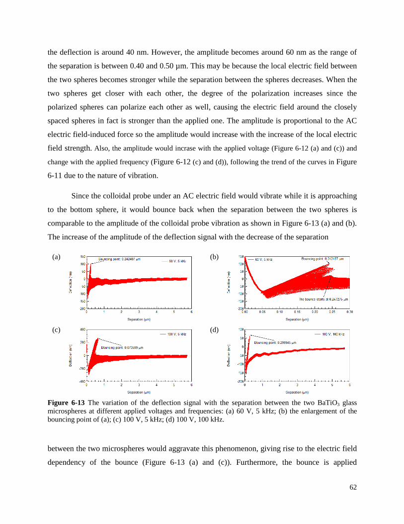
62
the deflection is around 40 nm. However, the amplitude becomes around 60 nm as the range of
the separation is between 0.40 and 0.50 µm. This may be because the local electric field between
the two spheres becomes stronger while the separation between the spheres decreases. When the
two spheres get closer with each other, the degree of the polarization increases since the
polarized spheres can polarize each other as well, causing the electric field around the closely
spaced spheres in fact is stronger than the applied one. The amplitude is proportional to the AC
electric field-induced force so the amplitude would increase with the increase of the local electric
field strength. Also, the amplitude would incrase with the applied voltage (Figure 6-12 (a) and (c)) and
change with the applied frequency (Figure 6-12 (c) and (d)), following the trend of the curves in Figure
6-11 due to the nature of vibration.
Since the colloidal probe under an AC electric field would vibrate while it is approaching
to the bottom sphere, it would bounce back when the separation between the two spheres is
comparable to the amplitude of the colloidal probe vibration as shown in Figure 6-13 (a) and (b).
The increase of the amplitude of the deflection signal with the decrease of the separation
(a)
(b)
(c)
(d)
Figure 6-13 The variation of the deflection signal with the separation between the two BaTiO3 glass microspheres at different applied voltages and frequencies: (a) 60 V, 5 kHz; (b) the enlargement of the bouncing point of (a); (c) 100 V, 5 kHz; (d) 100 V, 100 kHz.
between the two microspheres would aggravate this phenomenon, giving rise to the electric field
dependency of the bounce (Figure 6-13 (a) and (c)). Furthermore, the bounce is applied

63
frequency-dependent as well due to the frequency-dependent amplitude as shown above. In
Figure 6-12, we point out where the colloidal probe would bounce back, which is referred to as
“bouncing point” and summarize them at some conditions in Table 6-1. At a fixed applied
frequency, the bouncing point increases with the applied voltage. At a fixed applied voltage, the
bouncing point would increase with the applied frequency when it is below or equal to the
resonant frequency of the colloidal probe but decrease with the applied frequency when it is
above the resonant frequency, like the trend of curves in Figure 6-11. Note that there is no
apparent bounce as the applied frequency is 100 kHz. For example, the bouncing point is 295 nm
as the applied voltage is 100 V and the applied frequency is 100 kHz. Thus, we would discuss
the data at 100 kHz from 100 V to 30 V for the static components in the following sections since
this set is affected by the vibration of the colloidal probe much less. Also the smallest separation
we would concern is 300 nm.
Table 6-1 Brief summary of the bouncing point at different applied voltages and frequencies.
Applied Voltage and Frequency bouncing point (nm) 120, 100 kHz 869.54 100 V, 5 kHz 673.60
100 V, 100 kHz 299.95 60 V, 5 kHz 242.49
60 V, 100 kHz 153.89 30 V, 5 kHz None
30 V, 100 kHz None
6.3 Electric Field-Induced Force between Two Dielectric Microspheres
We measured the variation of the AC electric field-induced force ( inF ) with different
separations between the two BaTiO3 glass microspheres and different applied voltages/applied
electric field strengths ( 0E ) at different frequencies. Figure 6-14 shows the frequency
dependence of the field-induced force and the negative sign of the force means the measured
force is an attractive force. In Figure 6-14 (a), the field-induced force does not change with
frequency at different separations. In Figure 6-14 (b), there is no obvious variation of the field-
induced force from 1 kHz to 100 kHz at difference voltages. Thus, our results demonstrate that
the AC field-induced force between two dielectric microspheres at 1-100 kHz is independent of

64
(a)
(b)
Figure 6-14 (a) The variation of the AC electric field-induced forces with the separation between two BaTiO3 glass microspheres at different frequencies when the applied voltage is 60 V. (b) The variation of the AC electric field-induced forces with frequencies at different applied voltages when the separation between the two dielectric microspheres is 2.5 μm.
the frequency. Based on the Maxwell-Wagner model,5,12 the frequency-dependent term in the
Maxwell-Wagner model can be expressed by combining Eq. (3.21) and Eq. (3.22)
0.0 0.5 1.0 1.5 2.0 2.5 3.0 3.5-120
-110
-100
-90
-80
-70
-60
-50
-40
-30
-20
60 V 10 kHz 20 kHz 30 kHz 40 kHz 50 kHz 60 kHz 70 kHz 80 kHz 90 kHz 100 kHz
Separation (µm)
Forc
e (n
N)
0 20 40 60 80 100
-100
-80
-60
-40
-20
0
20
40
Forc
e (n
N)
Freqeuency (kHz)
2.5 µm 100 V 60 V 30 V

65
2 2 2
22 2 2
( ) ( )( 2 ) ( 2 )
p m p meff
p m p m
σ σ ω ε εβ
σ σ ω ε ε− + −
=+ + +
(6.3)
Since the dielectric constant of BaTiO3 glass microspheres25, 54,V
2effβ
and the range of the frequency
we used are quite high, we can ignore the terms of conductivity in Eq. (6.4), resulting in
independent of the frequency. In addition, the frequency-dependent terms in Colver’s model31
(Eq. (3.35)) can be neglected as well due to the large dielectric constant of BaTiO3 and applied
frequencies. Hence, our results about frequency dependence of the AC field-induced force agree
not only with Maxwell-Wagner model but also with Colver’s model. Although some research
results31,10 demonstrate that the AC field-induced force is frequency-dependent, the range of the
frequencies they used is so small that the conductivity would dominate the field-induced force,
not the dielectric constant. Some charges would easily accumulate at the material surfaces under
a low-frequency or DC field; that is the Maxwell-Wagner interfacial Relaxation,7,27 causing the
time-varying field-induced force even if the humidity is well-controlled.
To verify that our results do not have the Maxwell-Wagner interfacial relaxation, we
measured the variation of the field-induced force with time when the colloidal probe was
positioned around 6 μm above the bottom microsphere and hovered for over 100 seconds.18 We
also measured the force without any electric field as a reference. Figure 6-15 shows our results of
examining on Maxwell-Wagner Relaxation effect. In Figure 6-15 (a) and (b), the force varies
with time as a DC field is applied but the force maintains constant as 1 kHz electric field is
applied. This examination points out that the permittivities of the particles and the medium
dominate the field-induced force, not their conductivities under the applied AC field in our
experiment, implying the crossover frequency is lower than the 1 kHz for our system. We also
study the effect of the electric field strength on the rate of the charge accumulation by comparing
the variation of the normalized force with time (Figure 6-15 (c)). Surprisingly, there is no big
difference when the applied voltage is doubled. The above examination and analysis of the
Maxwell Wagner Relaxation effect suggests that AFM has potential to quantitatively study this V The BaTiO3 glass microspheres we used are not made of BaTiO3. The composition (by weight) of the microspheres is SiO2 (1~20%), B2O3 (1~20%), ZrO2 (1~10% ), BaO (40~70% ), and TiO2 (40~70%).54(a) Thus the relative permittivity of the particle we used may be less than 8054(b) but still much higher than that of air and of cantilever. And the electrical conductivity of oxides are usually quite low (< ~10-3 S/m)54(c). Further, BaTiO3 is ferroelectric so the special phenomena of the ferroelectric materials under an electric field are not taken into account here since the microspheres are not made of ferroelectric materials.

66
effect at micro- and/or nanoscale, which may help the study of high-dielectric electronic
materials.55
(a)
(b)
(c)
Figure 6-15 The variations electric field-induced force between two dielectric microspheres with time when the applied voltage is (a) 60 V and (b) 120 V and the distance between the two spheres is around 6 μm. The electric fields were applied after AFM started to record the data for about 5 seconds. (c) The variation of normalized DC electric field-induced force with time at difference applied voltages.
Beside the frequency dependence, we have also studied the relationship between the
field-induced force and the applied electric field strength at different separations as shown in
Figure 6-16. Our analyses manifest that the field-induced force would increase with the applied

67
voltage/electric field strength. In addition, the shorter the separation between the two
microspheres is, the lager the field-induced force is. To elucidate the relationship between the
filed-induced force and the electric field strength for two closely spaced dielectric microspheres,
we choose to plot the field-induced force versus the square of the applied electric field strength
(Figure 6-16). Surprisingly, the plotted curves exhibit linearity even when the separation is two
orders smaller than the diameter of the microsphere. Although according to the Maxwell-Wagner
model (Eq. (3.20)) the field-induced force should be proportional to the square of the applied
electric field strength, the model is , however, derived from the concept of the point-dipole
approximation, which is legitimate when the separation between the spheres is more than one
diameter.56
Figure 6-16 Relationship of the electric field-induced forces between two BaTiO3 glass microspheres with the square of the applied electric field at different separation as the applied frequency is 100 kHz.
To further study this, we also compare our results with the theoretical calculation from
two analytical models, the Maxwell-Wagner model and Colver’s equivalent circuit model as
shown in Figure 6-17. The calculated forces are smaller than the experimental results. The
discrepancy is expectable since the local electric field (i.e., the electric-field distribution around
the region where spheres are going to contact each other) for the closely spaced spheres is much
0 50 100 150 200 250 300-300
-250
-200
-150
-100
-50
0
0 2450 4900 7350 9800 12250 14700
3.0 µm 2.5 µm 2.0 µm 1.0 µm 500 nm 300 nm
E2 (V2/mm2)
Forc
e (n
N)
V2

68
higher than the applied electric field ( 0E ).57 Therefore, we conclude that the electric field around
the microsphere is indeed distorted and enhanced due to the small separation between the two
spheres.
(a)
(b)
Figure 6-17 (a) Comparison of the measured electric field-induced force with calculated results from different models and the fit to a simple power law, 2
0/ bcF E a x −= ⋅ , where a and b are constants and
b=0.5671. (b) The enlargement of (a) at small separation.
0.0 0.5 1.0 1.5 2.0 2.5 3.0-7
-6
-5
-4
-3
-2
-1
0
F/E2 0 (
nN⋅m
m2 /V
2 )
Separation (µm)
Experiment (30 V, 100 kHz) Maxwell-Wagner Model Colver's Model F/E2
0=a⋅xbc
Adj-R2=0.98
0.0 0.1 0.2 0.3 0.4 0.5-7
-6
-5
-4
-3
-2
-1
0
F/E2 0 (
nN⋅m
m2 /V
2 )
Separation (µm)
Experiment (30 V, 100 kHz) Maxwell-Wagner Model Colver's Model F/E2
0=a⋅xbc
Adj-R2=0.98

69
Note that the simulated curve from Colver’s model is closer to the experimental data than
that from the Maxwell-Wagner model when the separation is around 350 nm. The main
difference between these two models is that the field-induced force is inversely proportional to
the fourth power of the distance between the centers of the two spheres in the Maxwell-Wagner
model but in Colver’s model, the field-induced force is inversely proportional to the square of
the separation between the two spheres (i.e, from the bottom of the sphere to the top of the other
sphere).
Although we do not have a good theoretical model for the force, we have examined the
fit to a simple power law, 20/ b
cF E a x −= ⋅ where a and b are fitting constants. A good fit is
obtained when 0.5671b = , even at small separation, as shown in Figure 6-18.
Figure 6-18 The linearity between ln F and ln cx .
6.4 Electric Field-Induced Adhesion Force The field induced force increases in magnitude as the separation decreases but we are
unable to measure the force at very small separations because the spring becomes mechanically
unstable. One additional point that is experimentally accessible is the force at zero separation,
which can be obtained by bringing the spheres into contact and measuring the force required to
0.02 0.05 0.14 0.37 1.00 2.72
0.37
1.00
2.72
30 V, 100 kHz
ln xc (µm)
ln F
(nN)

70
Figure 6-19 The variation of the AC electric field-induced adhesion with different applied frequencies when the applied voltages are 100, 60 and 30, respectively. The dash lines represent the average values of each set of data.
pull them apart. This is the adhesion force, which has many applications in particle removal,
friction, resistance to disruption of particle aggregates, etc. We measured the adhesion for both
the DC force and the AC force. First, we examined the frequency dependence of the AC force.
The oscillatory response makes interpretation of this measurement more complicated because the
oscillation will make it easier for the particle to pull off the surface. Figure 6-19 shows that the
force is mainly independent of frequency, as for the forces at finite separation. There is a large
amount of scatter at low frequency, but we could not determine a consistent trend.
Figure 6-20 (a) shows the adhesion forces with and without field. When the field was off,
the measured adhesion force can range from -700 nN to -1200 nN. The possible reasons for such
large deviation are that the contact charges were generated while the colloidal probe was used to
scan the bottom sphere for finding the apex of the bottom sphere and the two spheres contected
during the force measurement no matter the field was on or off. Bunker et al. have studied the
electrostatic force between a lactose microsphere and a glass slide by AFM in these two
situations at different humidity: i) repeatedly contacting the particle with the glass slide in the
0 20 40 60 80 100-80
-60
-40
-20
-600
-400
-200
-160
-140
-120
-100
30 V
Applied Freuqnecy, f0 (kHz)
Elec
tric
Fiel
d-In
duce
d Ad
hesio
n Fo
rce
(nN)
100 V
60 V

71
(a)
(b)
Figure 6-20 (a) Adhesion force with field on and off. The solid spots means field off and the hollow spot means field on. (b) Correlation between the number of time of two spheres contact and the adhesion force.
normal direction by taking force-distance curves (contact charging) and ii) scanning the particle
across the surface of glass slide in contact mode imaging (tribocharging).58 They found both the
contact charging and tribocharing would generate contact charge at the surface at 0.1% RH. In
addition, the more the time that two spheres contacted, the higher the electrostatic force is. We
20 40 60 80 100 120
-1800
-1600
-1400
-1200
-1000
-800
-600
No field (AC) 100 kHz No field (DC) DC field
Applied Voltage (V)
Adhe
sion
Forc
e (n
N)
-1000
-950
-900
-850
-800
-750
-700 No field
Number of contact
Adhe
sion
Forc
e (n
N)
~50 ~450
R2=0.7317

72
also found similar qualitative results in our system as shown in Figure 6-19 (b). This hypothesis
corresponds to the existence of the peak at 0f in the FFT spectra of dynamic component as well.
Due to the possible existence of contact charges at the sphere surface, we subtract the adhesion
force without the field from the adhesion force with the field to get the field-induced adhesion
force as shown in Figure 6-21. Figure 6-21 shows the electric field dependence of the electric
field-induced adhesion force for the AC applied field and for the DC applied field. For both of
these fields, the adhesion is proportional to the square of the field strength, as for the force at a
finite separation, which implies that its origin is DEP (Figure 6-16). The important point is that
the adhesion can be systematically varied by the application of an electric field, and increased
greatly compared to the adhesion in the absence of a field. Note also that the DC-induced
adhesion is greater than the AC-induced adhesion. This result plus the dependence on the square
of the field is again consistent with results at finite separation so we again attribute the force to
accumulation of charges at the surface (the Maxwell-Wagner relaxation effect).
Figure 6-21 Relationship between the electric field-induced adhesion force and the square of the applied electric field strength under a DC and an AC electric field, where the frequency of the AC field is 100 kHz. The dash lines are the linear fitting results.
0 50 100 150 200 250 300 350-800
-700
-600
-500
-400
-300
-200
-100
0
AC field (100 kHz) DC field
E2 (V2/mm2)
Elec
tric
Fiel
d-In
duce
d Ad
hesio
n Fo
rce
(nN)
73
Chapter 7 – Conclusions We developed a quantitatively technique to measure the forces of two dielectric
microspheres induced by an external electric field in a low humidity environment by AFM.
Different from other proposed techniques, AFM can precisely control the relative position of the
microspheres, thus able to study the relationship between electric field-induced force and the
separation between two spheres, which is scarcely studied due to the limitation of the
measurement technique.
By the technique we developed, we measured the electric field-induced force and electric
field-induced adhesion force between two BaTiO3 glass microspheres under a DC and an AC
electric field in a very low humidity environment (less than 5% RH). We found that the DC
electric field-induced force of two spheres at a fixed separation would increase with time,
demonstrating the existence of the Maxwell-Wagner relaxation effect in a novel method and
exhibiting the potential of AFM to study dielectric properties of dielectric materials at micro-
and/or nanoscale. In addition, our results show that the AC electric field-induced force would not
change with the applied frequency ranged from 1 to 100 kHz, implying the crossover frequency
of the system we studied is below 1 kHz and the permittivities of the BaTiO3 glass microspheres
and the medium (i.e., dry air) dominate the field-induced force. Surprisingly, the AC electric
field-induced force is still proportional to the square of the applied electric field strength even
when the separation between two spheres is much smaller than the diameter of the microsphere
at which the local electric field would be distorted. Compared to the calculated results from the
Maxwell-Wagner model that is derived from the concept of the point-dipole approximation, the
measured AC field-induced force is much larger especially when the separation between the
spheres is very small, indicating that the local electric field around the closely spaces spheres is
indeed distorted. We also compared experimental results with other calculated results from
Colver’s equivalent circuit model. Interestingly, the results from Colver’s model are closer to the
experimental results than those from the Maxwell-Wagner model while the separation between
the spheres is small, implying the field-induced force is a very long-range force than the present
theories predict.

74
There is also an oscillatory component to the field-induced force. This force occurs at a
frequency of twice the field frequency and scales with the square of the field amplitude. It is
therefore consistent with a DEP force. The amplitude also grows as the separation decreases.
Finally, there is a large adhesion between the particles both in the absence of the field and
in the presence of the field. The additional force caused by the field has similar properties to the
force at a distance: it is independent of the frequency and scales with the square of the field
amplitude. The field is thus a useful method of controllably holding particles together in air.

75
References 1. Feng, J. Q.; Hays, D. A., Relative importance of electrostatic forces on powder particles.
Powder Technology 2003, 135, 65-75.
2. Rosensweig, R. E., PROCESS CONCEPTS USING FIELD-STABILIZED 2-PHASE
FLUIDIZED FLOW. Journal of Electrostatics 1995, 34 (2-3), 163-187.
3. Andres, U., Dielectric separation of minerals. Journal of Electrostatics 1996, 37 (4), 227-
248.
4. Hao, T., Electrorheological suspensions. Advances in Colloid and Interface Science 2002,
97 (1-3), 1-35.
5. Parthasarathy, M.; Klingenberg, D. J., Electrorheology: Mechanisms and models.
Materials Science & Engineering R-Reports 1996, 17 (2), 57-103.
6. Pethig, R., Review Article-Dielectrophoresis: Status of the theory, technology, and
applications. Biomicrofluidics 2010, 4 (2).
7. Jones, T. B., Electromechanics of Particles. Cambridge University Press: New York City,
NY, 1995.
8. Tombs, T. N.; Jones, T. B., DIGITAL DIELECTROPHORETIC LEVITATION. Review
of Scientific Instruments 1991, 62 (4), 1072-1077.
9. Wang, Z. Y.; Peng, Z.; Lu, K. Q.; Wen, W. J., Experimental investigation for field-
induced interaction force of two spheres. Applied Physics Letters 2003, 82 (11), 1796-1798.
10. Wang, Z. Y.; Shen, R.; Niu, X. J.; Lu, K. Q.; Wen, W. J., Frequency dependence of a
field-induced force between two high dielectric spheres in various fluid media. Journal of
Applied Physics 2003, 94 (12), 7832-7834.
11. Wang, Z. Y.; Shen, R.; Niu, X. J.; Sun, G.; Lu, K. Q.; Hou, B.; Wen, W. J., Dielectric
dependence of field-induced interspherical force. Journal of Physics D-Applied Physics 2005, 38
(8), 1325-1329.
12. Rankin, P. J.; Klingenberg, D. J., The electrorheology of barium titanate suspensions.
Journal of Rheology 1998, 42 (3), 639-656.
13. Mittal, M.; Lele, P. P.; Kaler, E. W.; Furst, E. M., Polarization and interactions of
colloidal particles in ac electric fields. Journal of Chemical Physics 2008, 129 (6).
14. Wei, M. T.; Junio, J.; Ou-Yang, H. D., Direct measurements of the frequency-dependent
dielectrophoresis force. Biomicrofluidics 2009, 3 (1).

76
15. Hong, Y.; Pyo, J. W.; Baek, S. H.; Lee, S. W.; Yoon, D. S.; No, K.; Kim, B. M.,
Quantitative measurements of absolute dielectrophoretic forces using optical tweezers. Optics
Letters 2010, 35 (14), 2493-2495.
16. Jonas, A.; Zemanek, P., Light at work: The use of optical forces for particle manipulation,
sorting, and analysis. Electrophoresis 2008, 29 (24), 4813-4851.
17. Neuman, K. C.; Nagy, A., Single-molecule force spectroscopy: optical tweezers,
magnetic tweezers and atomic force microscopy. Nature Methods 2008, 5 (6), 491-505.
18. Mizes, H. A., ADHESION OF SMALL PARTICLES IN ELECTRIC-FIELDS. Journal
of Adhesion Science and Technology 1994, 8 (8), 937-951.
19. Mizes, H.; Ott, M.; Eklund, E.; Hays, D., Small particle adhesion: measurement and
control. Colloids and Surfaces a-Physicochemical and Engineering Aspects 2000, 165 (1-3), 11-
23.
20. Kwek, J. W.; Vakarelski, I. U.; Ng, W. K.; Heng, J. Y. Y.; Tan, R. B. H., Novel parallel
plate condenser for single particle electrostatic force measurements in atomic force microscope.
Colloids and Surfaces a-Physicochemical and Engineering Aspects 2011, 385 (1-3), 206-212.
21. Gouveia, R. F.; Galembeck, F., Electrostatic Charging of Hydrophilic Particles Due to
Water Adsorption. Journal of the American Chemical Society 2009, 131 (32), 11381-11386.
22. Shamai, R.; Andelman, D.; Berge, B.; Hayes, R., Water, electricity, and between ... On
electrowetting and its applications. Soft Matter 2008, 4 (1), 38-45.
23. Gomez-Monivas, S.; Saenz, J. J.; Calleja, M.; Garcia, R., Field-induced formation of
nanometer-sized water bridges. Phys. Rev. Lett. 2003, 91 (5).
24. Kao, K. C., DIELECTRIC PHENOMENA IN SOLIDS: With Emphasis on Physical
Concepts of Electronic Processes. Academic Press: Amsterdam ; Boston, 2004.
25. Laughton, M. A.; Warne, D. F., Electrical Engineer's Reference. Newnes: Boston, 2003.
26. Lorrain, P.; Corson, D. R.; Lorrain, F., Fundamentals of Electromagnetic Phenomena.
W.H. Freeman: New York, 2000.
27. Morgan, H.; Green, N. G., AC Electrokinetics: colloids and nanoparticles. Research
Studies Press: Philadelphia, PA, 2003.
28. Hao, T.; Kawai, A.; Ikazaki, F., Mechanism of the electrorheological effect: Evidence
from the conductive, dielectric, and surface characteristics of water-free electrorheological fluids.
Langmuir 1998, 14 (5), 1256-1262.

77
29. Hughes, M. P., Nanoelectromechanics in Engineering and Biology. CRC Press: Boca
Raton, Fla, 2003.
30. Nilsson, J. W.; Riedel, S., Electric Circuits. 7th ed.; Pearson/Prentice Hall: Upper Saddle
River, N.J., 2005.
31. Colver, G. M., An interparticle force model for ac-dc electric fields in powders. Powder
Technology 2000, 112 (1-2), 126-136.
32. Bhushan, B.; Fuchs, H., Applied Scanning Probe Methods. Springer: Berlin ; New York,
2009; Vol. I-XIII.
33. Butt, H. J.; Cappella, B.; Kappl, M., Force measurements with the atomic force
microscope: Technique, interpretation and applications. Surface Science Reports 2005, 59 (1-6),
1-152.
34. Ralston, J.; Larson, I.; Rutland, M. W.; Feiler, A. A.; Kleijn, M., Atomic force
microscopy and direct surface force measurements - (IUPAC technical report). Pure and Applied
Chemistry 2005, 77 (12), 2149-2170.
35. (a) Fumagalli, L.; Ferrari, G.; Sampietro, M.; Gomila, G., Quantitative Nanoscale
Dielectric Microscopy of Single-Layer Supported Biomembranes. Nano Letters 2009, 9 (4),
1604-1608; (b) Gramse, G.; Casuso, I.; Toset, J.; Fumagalli, L.; Gomila, G., Quantitative
dielectric constant measurement of thin films by DC electrostatic force microscopy.
Nanotechnology 2009, 20 (39).
36. Attard, P., Measurement and interpretation of elastic and viscoelastic properties with the
atomic force microscope. Journal of Physics-Condensed Matter 2007, 19 (47).
37. Bhushan, B., Nanotribology and Nanomechanics. Springer: Berlin, 2011; Vol. I & II.
38. Sone, H.; Fujinuma, Y.; Hosaka, S., Picogram mass sensor using resonance frequency
shift of cantilever. Japanese Journal of Applied Physics Part 1-Regular Papers Short Notes &
Review Papers 2004, 43 (6A), 3648-3651.
39. (a) Dagata, J. A.; Perez-Murano, F.; Martin, C.; Kuramochi, H.; Yokoyama, H., Current,
charge, and capacitance during scanning probe oxidation of silicon. I. Maximum charge density
and lateral diffusion. Journal of Applied Physics 2004, 96 (4), 2386-2392; (b) Dagata, J. A.;
Perez-Murano, F.; Martin, C.; Kuramochi, H.; Yokoyama, H., Current, charge, and capacitance
during scanning probe oxidation of silicon. II. Electrostatic and meniscus forces acting on
cantilever bending. Journal of Applied Physics 2004, 96 (4), 2393-2399.

78
40. Jalili, N.; Laxminarayana, K., A review of atomic force microscopy imaging systems:
application to molecular metrology and biological sciences. Mechatronics 2004, 14 (8), 907-945.
41. Schirmeisen, A.; Anczykowski, B.; Hölscher, H.; Fuchs, H., Dynamic Modes of Atomic
Force Microscopy. In Nanotribology and nanomechanics. Volume 1, Measurement techniques
and nanomechanics, Bhushan, B., Ed. Springer: Berlin ; Heidelberg ; New York 2011; pp 307-
353.
42. Garcia, R.; Perez, R., Dynamic atomic force microscopy methods. Surface Science
Reports 2002, 47 (6-8), 197-301.
43. Melitz, W.; Shen, J.; Kummel, A. C.; Lee, S., Kelvin probe force microscopy and its
application. Surface Science Reports 2011, 66 (1), 1-27.
44. Sadewasser, S., Experimental Technique and Working Modes. In Kelvin probe force
microscopy: measuring and compensating electrostatic forces, Sadewasser, S.; Glatzel, T., Eds.
Springer-Verlag Berlin Heidelberg: Heidelberg ; New York, 2012; pp 7-24.
45. Israelachvili, J., Intermolecular & surface Forces. Academic Press London: London ;
San Diego 1991.
46. Senden, T. J., Force microscopy and surface interactions. Current Opinion in Colloid &
Interface Science 2001, 6 (2), 95-101.
47. Hutter, J. L.; Bechhoefer, J., CALIBRATION OF ATOMIC-FORCE MICROSCOPE
TIPS. Review of Scientific Instruments 1993, 64 (7), 1868-1873.
48. Honig, C. D. F.; Ducker, W. A., Squeeze Film Lubrication in Silicone Oil: Experimental
Test of the No-Slip Boundary Condition at Solid-Liquid Interfaces. J. Phys. Chem. C 2008, 112
(44), 17324-17330.
49. Figliola, R. S.; Beasley, D. E., Theory and Design for Mechanical Measurements. 5th ed.;
John Wiley: Hoboken, NJ 2011.
50. Senturia, S. D., Microsystem Design. Kluwer Academic Publishers: Boston, 2001.
51. Kaajakari, V., Practical MEMS: Design of microsystems, accelerometers, gyroscopes,
RF MEMS, optical MEMS, and microfluidic systems. Small Gear Publishing: 2009.
52. Kaler, K.; Jones, T. B.; Paul, R., LOW-FREQUENCY MICROMOTIONS OF DEP-
LEVITATED PLANT-PROTOPLASTS .1. Journal of Colloid and Interface Science 1995, 175
(1), 108-117.

79
53. Zhao, J. H.; Bridges, G. E.; Thomson, D. J., Direct evidence of "spring softening"
nonlinearity in micromachined mechanical resonator using optical beam deflection technique.
Journal of Vacuum Science & Technology A 2006, 24 (3), 732-736.
54. (a) Data sheet of barium-titanate spheres. Mo-Sci Corporation: Rolla, MO; (b) Robertson,
J., High dielectric constant oxides. European Physical Journal-Applied Physics 2004, 28 (3),
265-291.
55. Lunkenheimer, P.; Bobnar, V.; Pronin, A. V.; Ritus, A. I.; Volkov, A. A.; Loidl, A.,
Origin of apparent colossal dielectric constants. Physical Review B 2002, 66 (5).
56. Whittle, M.; Bullough, W. A.; Peel, D. J.; Firoozian, R., DEPENDENCE OF
ELECTRORHEOLOGICAL RESPONSE ON CONDUCTIVITY AND POLARIZATION
TIME. Physical Review E 1994, 49 (6), 5249-5259.
57. Chen, Y.; Sprecher, A. F.; Conrad, H., ELECTROSTATIC PARTICLE-PARTICLE
INTERACTIONS IN ELECTRORHEOLOGICAL FLUIDS. Journal of Applied Physics 1991,
70 (11), 6796-6803.
58. Bunker, M. J.; Davies, M. C.; James, M. B.; Roberts, C. J., Direct observation of single
particle electrostatic charging by atomic force microscopy. Pharmaceutical Research 2007, 24
(6), 1165-1169.


