Mecanique & Industries 10, 365–376 (2009) www.mecanique-industries.orgc© AFM, EDP Sciences 2009DOI: 10.1051/meca/2009070
Mecanique& Industries
Effect of manufacturing defects on the dynamic behaviourfor an helical two-stage gear system
Lassaad Walha, Yassine Drissa, Tahar Fakhfakh and Mohamed Haddar
Unit research of mechanical systems dynamics, National engineering school of Sfax, Tunisia
Received 11 March 2008, Accepted 6 August 2009
Abstract – The modelling of the dynamic behaviour of three-dimensional model of two-stage gear systemis formulated for general helical gears location. The excitation is induced by the periodic variation of themesh stiffnesses. This case describes the real working of the gearings. First, the modal analysis of the systemis treated. Then, the calculation of the dynamic response is performed by a step-by-step time integrationmethod (Newmark method). Finally, two types of manufacturing defects on the gears are introduced inthe model: eccentricity and profile defect. An analysis of the effects of these defects on the gear systemdynamic behaviour is then treated.
Key words: Helical two-stage gear / eccentricity /profile error
Resume – Effets des defauts de fabrication sur le comportement dynamique d’une transmis-sion par engrenage a deux etages a denture helicoıdale. La modelisation du comportement dyna-mique d’un modele spatial relative a une transmission par engrenage a deux etages a denture helicoıdaleest formulee pour une disposition generale des roues dans le carter. La principale source d’excitation est lavariation periodique de la raideur d’engrenement. Dans une premiere etude une analyse modale est traitee.Ensuite le comportement dynamique est determine grace a la methode de resolution numerique pas a pasdans le temps (methode de Newmark). Finalement, deux types de defauts de fabrication des roues sontintroduits dans le modele : defaut d’excentricite et defaut de profil. L’analyse des effets de ces defauts surle comportement dynamique du systeme est etudiee.
Mots cles : Transmission a deux etages / denture helicoıdale / defaut d’excentricite / defaut de profil
1 Introduction
Gearing is actually the best solution to transmit ro-tational motions and couple which has been offered nu-merous advantages [1]: it ensures a mechanical reliabilityand its mechanical efficiency is of the order of 0.96 to0.99. But today, several applications inquire for the gear-ing transmissions to be more and more reliable, light andhaving long useful life that requires the control of theacoustic broadcast and the vibratory behaviour of thesegearings [2].
The literature is rich by theoretical and experimentalworks achieved on the gearings. Several problems havetreated on the one stage gear system [3, 4]. Yakhou [5]worked on the helical teeth in the gearboxes. He men-tionned the different origins of the noises radiated bythese boxes. He introduced in the model the casing andthe rolling bearings. His work was validated by an exper-imental part. Perret-Liaudet [6] introduced some flexible
a Corresponding author: [email protected]
shafts in his one stage gear model. To solve the dynam-ics response of the system, he used an iterative spectralmethod that permits to reduce the time of the calculation.
The works of research [6–14] included the differenttypes of defects that may affect the gearings. Indeed, theresearchers are interested in the gearing defects allowingthem to be able to analyze the dynamic behaviour of thetransmission in presence of these defects. Parker et al. [15]treated a plane problem of two-stage gear systems consti-tuted by three toothed wheels without introducing nei-ther the flexibility of the bearing nor the shaft one. Theywere interested in the problem of instabilities in these sys-tems. However, the previous investigations have treatedonly models of two-stage gear systems with spur gear. Inthis paper, a three-dimensional model of two-stage gearsystems in permanent working state is developed. Then,the numeric results concerning the dynamic response areobtained thanks to an algorithm of numerical integra-tion (Newmark algorithm [8]). Finally, the cases of perfectand defected gearbox with two geometric defects are thenstudied.
Article published by EDP Sciences

366 L. Walha et al.: Mecanique & Industries 10, 365–376 (2009)
Nomenclature
[C] proportional damping matrix
Eptot potential energy coming from the misalignment
fei mesh frequencies (Hz)
{F0} external force vector
h mesh phasing
j j = 1 to 3; number of the block
kφj , kψj bending stiffness of the bearing j (N/m)
kxj , kyj , kzj traction-compression stiffness of the bearing j (N.m/rad)
kθj torsional stiffness of the shaft j (N/m)
[Ks] average stiffness matrix of the structure
[K(t)] gear mesh stiffness matrix
[KC] mean matrix component
[KV] time mesh stiffness varying matrix component with zero average[K
]global average stiffness matrix of the model
Lmax maximal length of contact line (N/m)
Lmin minimal length of contact line (N/m)
[M] time independent system mass matrix
{q} generalised coordinate’s vector
{qS} , {qd} static and dynamic components of the generalised coordinate’s vector
Rbij basic radius of the wheel i related to block j (m)
xj , yj , zj translational displacements of the bearing j (N/m)
Zij teeth numbers of the gears (ij)
αi pressure angles (◦)β helix angle (◦)χ angle between the center lines which locates the second stage relatively to the first (◦)γi angle that the line of the gear centers makes with the stationary axis (◦)δs teeth deflections (s = 1, 2) (m)
εα contact ratio
εβ overlap ratio
2 Model of the two-stage gear system
Two-stage gear system is composed of two trains ofgearings. Every train links two blocks. So, the gear systemhas in totality three blocks (j = 1 to 3) [5,16]. Every block(j) is supported by flexible bearing the stiffness of whichkxj , kyj , kzj , kφj and kψj are the traction-compressionand the bending stiffness [17]. Moreover, the shafts (j) areonly submitted to the torsional motion and admit sometorsional stiffness kθj. The wheels 11 and 32 character-ize respectively the motor side and the receiving machineside which inertias are Im and Ir [18]. The other helicalgears constitute the gearbox. The gear meshes are mod-elled by linear spring along the lines of action (Fig. 1). xj ,yj and zj are supposed the translational displacements ofthe bearing. The shaft lengths are considered of the sameorder of the teeth width. Moreover, it is assumed that themasses of shafts are negligible.
3 Mesh stiffness variation modelling
The meshes stiffness variations k1(t) and k2(t) aremodelled by trapezoidal waves that depend on the fea-tures of the gearings [18]. It is proportional to the length
of contact line. The basic length l′ (Fig. 2), the contactratio εα and the overlap ratio εβ are defined by [18]:
l′ = (P 2b + P 2
x )1/2; (1)εα = L/Pb=A+a; (2)
εβ= l′/Px=B+b; (A,B : real parts, a, b : decimal parts)(3)
The maximal length Lmax and the minimal length Lmin
(Fig. 3) are defined as follows:
Lmax = (AB +Ab+ aB + c)l′; (4)
if (a+ b) > 1 : Lmin = (AB +Ab+ aB + (a+ b− 1))l′;(5)
if (a+ b) < 1 : Lmin = (AB +Ab+ aB)l′;With c the smallest of a and b
(6)
εαi are the contact ratios (i = 1, 2). Mesh frequencies feiare related by the following relation [15]:
fe2 =Z22
Z21fe1 (7)
Z21 and Z22 represent the teeth numbers of the gears (21)and (22). The term pi represents “the initial phasing” for

L. Walha et al.: Mecanique & Industries 10, 365–376 (2009) 367
Gear 12
Wheel 32
Gear 21 Gear 22
Wheel 11
Gear 31
ky3kx3
kz3
kz2
kx2
ky1kx1
kz1
k1(t)
k2(t)
kθ2
kθ1
11θ
1k φ
kθ3
ky2
1k ψ
2kψ
2k φ
3k φ
3k ψ
12θ
21θ
22θ
31θ32θ
Fig. 1. Model of the two-stage gear system.
Fig. 2. Traces of the contact line in the action plan [18].
the mesh stiffness on the stage i. Mesh phasing h betweenthe two mesh stiffness 1 and 2 (Fig. 9) is expressed by [15]:
h =χZ22
2π(8)
χ represents the angle between the lines of the centres andlocates the second stage relatively to the first. To simplify
Time
Length of the contact line
L
L
a-b tc t c t (1-a-b) t
t = Te
max
min
Fig. 3. Modelling of the mesh stiffness variation of the helicalgear [18].
31
O12
O31
O21 γ2
γ10X
r
2122
12
11
32
0Yur
0Yur
0Xr
α1
α2
Fig. 4. Positions of the wheels of the helical two stage-gearsystem.
the problem, it is supposed that γ1 = 0◦ (Fig. 4), then χis expressed by:
χ = π − γ2 (9)
4 Equations of motion
The positions of the wheels of the helical two stage-gear system are represented by Figure 4. αi are the pres-sure angles. Every γi designates the angle that the line ofthe gear centers makes with the stationary axis
(O, �X0
).
4.1 Expression of the teeth deflections
The generalised coordinate’s vector {q} includestwenty-one degrees of freedom. Indeed, each block j hasseven degrees of freedom: five degrees (xj , yj , zj, φj , ψj)corresponding to the bearing j displacements (threetranslations and two rotations) and two degrees (θ1j , θ2j)corresponding to the wheels (1) and (2) of the shaft j(due to the above hypothesis):
{q} = {x1, y1, z1, x2, y2, z2, x3, y3, z3, φ1, ψ1, φ2, ψ2,
φ3, ψ3, θ11, θ12, θ21, θ22, θ31, θ32} (10)

368 L. Walha et al.: Mecanique & Industries 10, 365–376 (2009)
basic circle of wheel 21
basic circle of wheel 12
action plan
line of contact
γ1
α1
k1(t)
p1 p2
2xuur
2yuur
2xuur
1xur
1yuur
2zuur
1zur
β1Q 1 2Q Quuuuur
2Q
zr
l1, l2
1nur
1Q
2Q
Basic circle of gear 21
Basic circle of gear 12
Fig. 5. Modelling of the connection between gear (12) and gear (21).
Table 1. Constants appearing in the expression of δ1(l, t).
s1 cos β sin(γ1 − α1)
s2 cos β cos(γ1 − α1)
s3 sin β
s4 −l cos2 β cos(γ1 − α1) + sin β(−Rb12 sin(α1 − γ1) + cos(γ1 − α1)(p1 − l sin β))
s5 −l cos2 β sin(γ1 − α1) − sin β(Rb12 cos(α1 − γ1) + sin(γ1 − α1)(l sin β − p1))
s6 Rb12 cos β
s7 l cos2 β cos(γ1 − α1) − sin β(Rb21 sin(α1 − γ1) − cos(γ1 − α1)(p2 + l sin β))
s8 l cos2 β sin(γ1 − α1) + sin β(−Rb21 cos(α1 − γ1) + sin(γ1 − α1)(p2 + l sin β))
s9 Rb21 cos β
The first teeth deflection δ1(t) is written as follows(Fig. 5):
δ1(t) = Lδ1 {q} (11)
Lδ1 = [−s1 s2 s3 s1 −s2 −s3 0 0 0 s4 s5 s7 s8 0 0 0 s6 s9 0 0 0](12)
The constants si are given in Table 1. In this table, thedistances p1 and p2 are defined by:
p1 = Rb12 tgα1 ; p2 = Rb21 tgα1 (13)
Rbij is the basic radius of the wheel j related to block i.The second teeth deflection δ2(t) is supposed to be
defined by the product of L by {q} and written as follows(Fig. 6):
Lδ2 = [0 0 0 t1−t2 t3 −t1 t2 −t3 0 0 t4 t5 t7 t8 0 0 0 t6 t9 0 ](14)
The constants ti are given in Table 2. In this table, thedistances p′2 and p3 are defined by:
p3 = Rb22 tgα2 ; p4 = Rb31 tgα2 (15)
4.2 Matrix differential equation
Lagrange formalism leads to the set of differentialequations governing the system motion:
[M] {q} + [C] {q} + ([Ks] + [K(t)]) {q} = {F0} (16)
[M] represents the time independent system mass ma-trix. The average stiffness matrix of the structure is notedby [Ks].
[KS] =[Kp 00 Kθ
](17)
[Kp] can be written as follow:
[Kp] = diag(kx1, ky1, kz1, kx2, ky2, kz2, kx3, ky3, kz3) (18)

L. Walha et al.: Mecanique & Industries 10, 365–376 (2009) 369
basic circle of wheel 31
basic circle of wheel 22
action plan
line of contact
3xuur
3yuur
3zuur
2xuur
2yuur
1zur
2γ
2α
k2(t)
'2p 3p
β2Q 3Q
l2, l3
2Q
2 3Q Quuuuur
3Q
2nuur
Basic circle of gear 31
Basic circle of gear 22
Fig. 6. Modelling of the connection between gear (22) and gear (31).
Table 2. Constants appearing in the expression of δ2(l, t).
t1 cos β sin(α2 + γ2)
t2 cos β cos(α2 + γ2)
t3 sin β
t4 l cos2 β cos(α2 + γ2) + sin β(Rb22 sin(α2 + γ2) + cos(α2 + γ2)(l sin β − p3))
t5 l cos2 β sin(α2 + γ2) − sin β(Rb22 cos(α2 + γ2) + sin(α2 + γ2)(p3 − l sin β))
t6 −Rb22 cos β
t7 −l cos2 β cos(α2 + γ2) − sin β(−Rb31 sin(α2 + γ2) + cos(α2 + γ2)(l sin β + p4))
t8 −l cos2 β sin(α2 + γ2) + sin β(−Rb31 cos(α2 + γ2) − sin(α2 + γ2)(p4 + l sin β))
t9 −Rb31 cos β
[Kθ] is composed by shafts stiffness and it is expressed by:
[Kθ] =⎡⎢⎢⎢⎢⎢⎢⎢⎢⎢⎢⎢⎢⎢⎢⎢⎢⎣
kφ1 0 0 0 0 0 0 0 0 0 0 00 kψ1 0 0 0 0 0 0 0 0 0 00 0 kφ2 0 0 0 0 0 0 0 0 00 0 0 kψ2 0 0 0 0 0 0 0 00 0 0 0 kφ3 0 0 0 0 0 0 00 0 0 0 0 kψ3 0 0 0 0 0 00 0 0 0 0 0 kθ1 −kθ1 0 0 0 00 0 0 0 0 0 −kθ1 kθ1 0 0 0 00 0 0 0 0 0 0 0 kθ2 −kθ2 0 00 0 0 0 0 0 0 0 −kθ2 kθ2 0 00 0 0 0 0 0 0 0 0 0 kθ3 −kθ30 0 0 0 0 0 0 0 0 0 −kθ3 kθ3
⎤⎥⎥⎥⎥⎥⎥⎥⎥⎥⎥⎥⎥⎥⎥⎥⎥⎦
(19)
[K(t)] is the gearmesh stiffness matrix. It is a time varyingmatrix and can be expressed by:
[K(t)] = (Lδ1)T Lδ1k1(t) + (Lδ2)
T Lδ2k2(t) (20)
k1(t) ant k2(t) are the time varying mesh stiffness func-tions.
[K(t)] can then be written as:
[K(t)] = [KC] + [KV(t)] (21)
where [KC] is the mean matrix component, [KV(t)] is thetime varying matrix component with zero average.
It is noted that[K
]is the global average stiffness ma-
trix of the model. This time independent matrix is ex-pressed by: [
K]
= [KS] + [KC] (22)
[KS] is defined in equation (17).The vector {q} can be decomposed in static and dy-
namic components vector as:
{q} = {qS} + {qd} (23)
The pseudo static component {qS} is introduced by:[K
]{qS} = {F0} (24)

370 L. Walha et al.: Mecanique & Industries 10, 365–376 (2009)
Table 3. System parameters.
Material :42CrMo4 ρ = 7860 Kg.m−3
Motor characteristics
Motor torque Cm = 1000 N.m
Motor inertia Im = 3.5 × 10⁻⁴ Kg.m2
Motor speed Nm = 1500 rpm
Receiving characteristicsReceiving torque Cr = −2888 N.m
Receiving inertia Ir = 6.5 × 10⁻⁴ Kg.m2
Bearing stiffness kxi = 108 N.m−1 ; kyi = 108 N.m−1 ; kzi = 108 N.m−1
Shafts torsional stiffness kθi = 3 × 10⁵(N.m−1)/rad
First gearmesh Second gearmesh
Pressure angle αn = 20◦
Helix angle β = 20◦
Teeth module mn = 4 × 10⁻³ m
Teeth number Z12 = 18 ; Z21 = 26 Z22 = 20 ; Z31 = 40
Average mesh stiffness kmoy = 4108 N.m−1 kmoy = 4108 N.m−1
Contact ratio εα1 = 2.7 εα2 = 3.7
Covering ratio εβ1 = 1.09 εβ2 = 1.09
Teeth width b = 35 × 10−3 m
Where the external force vector {F0} can be written as:
{F0} = {0, 0, 0, 0, 0, 0, 0, 0, 0, 0, 0, 0, 0, 0, 0, Cm,0, 0, 0, 0,−Cr}T (25)
In this context, a proportional damping is considered andcan be expressed by: [19]
[C] = λ [M] + μ[K
](26)
where λ and μ are the damping constants defined by:
λ = μ = 0.03 (27)
The matrix differential equation governing the dynamiccomponent behaviour will then be written as:
[M] {qd}+[C] {qd}+([KS] + [K(t)]) {qd} = − [KV(t)] {qs}(28)
5 Modal analysis
Table 3 regroups the technological and dimensionalfeatures of the two-stage gear system. The frequencies andmodal deflections are determined while assimilating thematrix stiffness of the model to the average matrix notedby [K]. Table 4 regroups the first natural frequencies ofthe system for three locations of the wheels. The presenceof null frequency characterizing of rigid body motion isnoticed. Also, it is noted that the optimal position, whichoptimizes the conception of the two-stage gear system, isdefined by χ = 135◦.
Figures 7 and 8 represent some eigen modes of thewheels for the three cases of wheels location. The dashedlines indicate the initial wheels positions. The first modehas purely rotational motion and characterizes the rigid
Table 4. Eigen frequencies of the model.
Frequency χ = 180◦ χ = 135◦ χ = 80◦
h = 0 h = 0.5 h = 0.44
f1 0 0 0
f2 1660 1680 1720
f3 = f4 2080
f5 2270 2300 2380
f6 2530 2490 2440
f7 2610
f8 3690 3680 3620
f9= f10 4160
f11 6170 6120 5960
body motion. The sixth mode is a combined motion oftranslation and rotation. The ninth mode is a mode ofpure translational motion.
According to the Table 4, it is noticed that:
– the eigen frequencies f3 and f4 (respectively f9 andf10) are equal for every wheels positions. Moreover,it is noted that the eigen modes associated to thesefrequencies present only translational displacementsat the third bearing (respectively at the first one);
– the frequency f7 is independent of the position of thewheels.
6 Dynamic response for two-stage gearsystem without defects
The calculation of the dynamic response is performedby a step-by-step time integration method (Newmarkmethod). The step of integration is equal to 10−5 s.For the two-stage gear system without defects, the main

L. Walha et al.: Mecanique & Industries 10, 365–376 (2009) 371
Reference position First mode (Rigid body motion)
Sixth mode (f = 2530 Hz) Ninth mode (f = 4160 Hz)
12
11
22
2112
11
22
21
32
31
31
32
12
11
22
2112
11
22
21
32
31
32
1211
22
2112
11
22
21
32
31
31
32
1211
22
2112
11
22
21
32
31
32
31
31
Fig. 7. Typical vibration for the three types of modes for χ = 180◦.

372 L. Walha et al.: Mecanique & Industries 10, 365–376 (2009)
135χ = ° (f6 = 2490 Hz) 80χ = ° (f6 = 2440 Hz)
1211
22
2112
11
22
21
32
31
31
32
1211
2112
11
22
21
32
31
32
Fig. 8. Typical vibration for the Sixth mode.
0 1 2 3 4 5 6
x 10-3
2
2.5
3
3.5
4
4.5
5x 10
8
Time (s)
Stif
fnes
s (N
/m)
h
Fig. 9. Modelling of two mesh stiffness variation (–: k1(t);–:k2(t)).
sources of excitation are the two mesh stiffness variationsrepresented by Figure 9.
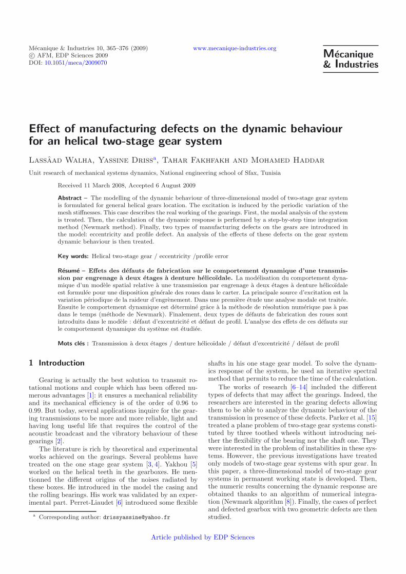
Figure 10 represents the frequency response of trans-lational displacements resulting on the first bearing. It isclearly noticed the presence of several peaks in every sig-nal. These peaks correspond to the two mesh frequenciesfe1 = 450 Hz and fe2 = 346 Hz with their harmonicsand other combined frequencies such as fe1 − fe2 andfe1 + fe2. The position which is defined by χ = 135◦,leads to the reduction of the gear system vibratory level.
7 Modelling of the defects
Most gearboxes include inherent defects followingtheir manufacture. These defects may increase whileworking. They are essentially:
– errors of tooth: perfectly conjugated deviations of aprofile of tooth, caused by imperfections of manufac-ture, or by a modification of profile;
– errors of manufacturing: as the eccentricity errors. . .
In this paper we try to approach two defects while sup-posing that they are the more met in the practice.
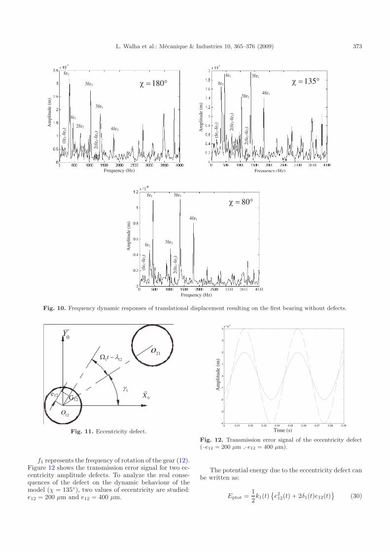
7.1 Modelling of the eccentricity defect
The transmission is now supposed having an eccen-tricity on gear (12). The eccentricity expresses the dis-tance between the theoretical and the real rotational axis(Fig. 11) belonging to the first train of the two-stage gearsystem. O12 and G12 represent respectively the rotationaland geometric centres of the gear (12). The eccentricitydefect is defined by the parameter e12, which representsthe distance between the axis, and by a phase λ12 to spec-ify the initial angular position.
An eccentricity defect causes teeth deflection on theirown line of action. The deflection δ1(t) is then added witha transmission error e12(t) defined by:
e12(t) = e12 sin(2πfd − λ12 − α1) (29)
fd is the frequency of defect. In our case, fd = f1.
L. Walha et al.: Mecanique & Industries 10, 365–376 (2009) 373
fe2
fe1
2fe2
3fe2
3fe1
(fe
1-fe
2)
2(fe
1-fe
2)
180χ = °
4fe2 2(fe
1-fe
2)
fe2
fe1
3fe2
3fe1
Frequency (Hz)
(fe
1-fe
2)
2(fe
1-fe
2)
135χ = °4fe1
fe2
fe1
3fe2
3fe1
Am
plitu
de (
m)
(fe
1-fe
2)
2(fe
1-fe
2)
80χ = °
4fe1
Frequency (Hz)
Am
plitu
de (
m)
Am
plitu
de (
m)
Frequency (Hz)
Fig. 10. Frequency dynamic responses of translational displacement resulting on the first bearing without defects.
80ψ = °
0Yuuur
0Xr1γ
1 12t λΩ −
12O
21o
e12 G12
Fig. 11. Eccentricity defect.
f1 represents the frequency of rotation of the gear (12).Figure 12 shows the transmission error signal for two ec-centricity amplitude defects. To analyze the real conse-quences of the defect on the dynamic behaviour of themodel (χ = 135◦), two values of eccentricity are studied:e12 = 200 μm and e12 = 400 μm.
0 0.01 0.02 0.03 0.04 0.05 0.06 0.07 0.08 0.09-4
-3
-2
-1
0
1
2
3
4x 10
-4
Time (s)
Am
plitu
de (
m)
Time (s)
Am
plit
ude
(m)
Fig. 12. Transmission error signal of the eccentricity defect(–e12 = 200 μm ,–e12 = 400 μm).
The potential energy due to the eccentricity defect canbe written as:
Eptot =12k1(t)
{e212(t) + 2δ1(t)e12(t)
}(30)

374 L. Walha et al.: Mecanique & Industries 10, 365–376 (2009)
f1
fe1-f1fe1+f1
2fe1-f1 2fe1+f1
Frequency (Hz)
Am
plitu
de N
) e12=200μm
e12=400μm
Am
plitu
de (
N)
Fig. 13. Time and spectrum varying external force due to the eccentricity defect.
0 200 400 600 800 1000 1200 1400 1600 1800 20000
1
2
3
4
5
6
7
8x 10
-7
Frequency (Hz)
Am
plitu
de (
m/H
z)
fe1
f1
fe1-f1
fe23fe2
fe1+f13fe1-f1
3fe1+f1
3fe1
2fe1
Am
plit
ude
(m)
Frequency (Hz)0 200 400 600 800 1000 1200 1400 1600 1800 2000
0
0.5
1
1.5
2
2.5
3
3.5
4x 10
-7
Frequency (Hz)
Am
plitu
de (
m/H
z)
fe1
f1fe1-f1
fe23fe2
fe1+f13fe1-f1
3fe1+f1
3fe1
2fe1
Frequency (Hz)
Am
plit
ude
(m)
e12 = 200 μm e12 = 400 μm
Fig. 14. Frequency dynamic response of the first bearing for eccentricity defect.
Then, the effect of the eccentricity defect can be expressedby the external force {Fpex(t)} given by:
{Fpex(t)} = k1(t)e12(t){−s1, s2, s3, s1,−s2,−s3, 0, 0, 0,s4, s5, s7, s8, 0, 0, 0, s6, s9, 0, 0, 0}T (31)
Figure 13 shows the time and the spectrum varying ex-ternal force due to the eccentricity defect. The spectrumsignal represents several peaks due to the modulating phe-nomenon resulting from eccentricity defect and mesh vari-ation (mfe1 ± nf1).
Figure 14 represents the dynamic displacementresponse spectrum of the first bearing for eccentricity de-fect.
The responses are characterized by the appearance ofsidebands around the first mesh frequency (fe1 = 450 Hz)and of its first harmonics. The appearance of a new peakbesides the signal is noticed, this peak corresponds to thedefect frequency (f1 = 25 Hz). The modulation ampli-tude will be more and more amplified when the value ofeccentricity is raised. This result is translated in the spec-trum by the amplitudes amplification of the sidebandsthat surround the mesh frequency. The second mesh fre-quency (fe2 = 346 Hz) will not be affected by the defectfor any value of eccentricity.
0Yuur
0Xuur1γ
1( )k t
12o
21o12
p (t)
Fig. 15. Profile error modelling.
7.2 Effect of a profile error on the dynamic response
Profile errors result in imperfections on the geometryof the teeth. It is characterized by a shape deviation be-tween the real profile and the theoretical profile of thetooth.
A profile error constitutes a source of important exci-tation in gearboxes. For similar teeth profiles error, theseexcitations are periodic of fundamental frequency equal tothe mesh frequency corresponding to the wheel affectedby this error.

L. Walha et al.: Mecanique & Industries 10, 365–376 (2009) 375
2fe1
fe1
4fe1
5fe1
3fe1
Am
plitu
de (
m)
2fe1
fe1
4fe1
5fe1
3fe1
Am
plitu
de (
m)
p12=100 μm p12=300 μm
Frequency (Hz) Frequency (Hz)
Fig. 16. Frequency responses of the first bearing with profile error (χ = 135◦).
As it is presented in the Figure 15, the defect of profileerror is introduced by the addition of a displacement typeterm p(t) to the tooth deflection on the line of action. Thiserror is supposed identical on all teeth for the gear (12).
Its variation is assimilated by:
p12(t) = p12 ++∞∑n=1
p12 sin(2 π n fe1 t) (32)
p12 and fe1 represent respectively the profile error valueand the first mesh frequency.
The profile error leads to a new external excitationexpressed by:
{Fpp(t)} = k1(t)∂δ1(t)∂qi
p12(t) (33)
{Fpp(t)} = k1(t)p12(t){−s1, s2, s3, s1,−s2,−s3, 0, 0, 0,s4, s5, s7, s8, 0, 0, 0, s6, s9, 0, 0, 0}T (34)
The profile error will amplify the amplitude of the trans-lational displacements on the three bearings. This resultis clear in the Figure 16.
8 Conclusion
In this paper, the helical two-stage gear system wasmodelled by twenty-one degrees of freedom system witha time varying stiffness matrix. In the first time, thedynamic behaviour of the two-stage gear system with-out defects was made. A step-by-step time integrationmethod (Newmark algorithm) was used to obtain this dy-namic behaviour. The frequency dynamic response showsthe domination of the peaks corresponding to the meshfrequencies. The dynamic response fluctuations are min-imum for the second wheels location (χ = 135◦) thatpermits to reduce the gearbox size.
The helical two-stage gear system behaviour is af-fected by manufacturing defects. An amplitude modula-tion occurs when an eccentricity defect is introduced. This
defect produced sidebands around the affected gearmeshfrequency and its first harmonics.
A profile error increases the vibratory level. These sur-veys allow getting an idea on the characterisation of thedynamic response of the helical two-stage gear system af-fected by manufacturing defects.
References
[1] G.W. Blankenship, R. Singh, Dynamic force transmis-sibility in helical gear pairs, Mechanism and MachineTheory 29 (2000) 212–228
[2] C. Bard, Modelisation du comportement dynamique destransmissions par engrenages, these de doctorat, InstitutNational des Sciences Appliquees de Lyon, INSAL 0031,1995
[3] P. Velex, M. Ajmi, On the modelling of excitations ingeared systems by transmission errors, J. Sound Vib., 290(2006) 882–909
[4] P. Velex, M. Ajmi, Dynamic tooth loads and quasi-statictransmission errors in helical gears – Approximate dy-namic factor formulae, Mechanism and Machine Theory42 (2007) 1512–1526
[5] K. Yakhou, Validation experimentale d’un modele dy-namique globale de boıte de vitesses automobile, Thesede l’Institut National des Sciences Appliquees de Lyon,2002
[6] Perret-Liaudet, Etude des mecanismes de transfert en-tre l’erreur de transmission et la reponse dynamique desboıtes de vitesses d’automobile, These de l’Ecole Centralede Lyon, 1992
[7] F. Chaari, T. Fakhfakh, R. Hbaieb, J. Louati, M. Haddar,Influence of manufacturing errors on the dynamics behav-ior of planetary gears, International Journal of AdvancedManufacturing Technology 27 (2005) 738–746
[8] G. Dhatt, G. Touzot, Une presentation de la methode deselements finis, edition Maloine, 1984
[9] M. Haddar, M. Ben Amar, W. Gafsi, A. Maalej, Analysedu comportement dynamique et tribologique d’une trans-mission a engrenages droits en presence d’un defaut deparallelisme, 3e journees de mecanique et ingenierie, Sfax,Tunisie, 2000

376 L. Walha et al.: Mecanique & Industries 10, 365–376 (2009)
[10] R. Hbaieb, F. Chaari, T. Fakhfakh, M. Haddar, Influenceof eccentricity, profile error and tooth pitting on helicalplanetary gear vibration, Machine Dynamics Problems,29 (2005) 5–32
[11] M. Lebold, K. McClintic, R. Cambell, C. Byington, K.Maynard, Review of vibration analysis methods for gear-box diagnostics and prognostics. Proceedings of the 54thMeeting of the Society for Machinery Failure PreventionTechnology, Virginia Beach, 2000
[12] G. Litak, M.I. Friswell, Vibrations in gear systems,Chaos, Solitons & Fractals 16 (2003) 145–150
[13] A.J. Miller, A new wavelet basis for the decomposi-tion of gear motion error signals and its application togearbox diagnostics, These de l’universite de l’etat dePennsylvanie, 1999
[14] K.P. Maynard, Interstitial processing: the applicationof noise processing gear fault detection. Proceedings ofthe international conference on Condition monitoring,University of Wales Swansea, UK, 1999, pp. 77-86
[15] G.R. Parker, J. Lin, Mesh Stiffness Variation Instabilitiesin Two–stage Gear Systems, Journal of vibration andacoustics, 124 (2002)
[16] L. Walha, J. Louati, T. Fakhfakh, M. Haddar, Effectsof eccentricity defect and tooth crack on two-stage gearsystem behaviour, International Journal of EngineeringSimulation 6 (2005) 17–24
[17] T. Eritenel, R.G. Parker, Modal properties of three-dimensional helical planetary gears, J. Sound Vib., InPress, Corrected Proof, Available online 10 April 2009
[18] M. Maatar, Contribution a l’analyse du comportementdynamique de reducteurs a engrenages simple etage,Influence des ecarts de forme et des defauts de montage,These de l’Institut National des Sciences Appliquees deLyon, 1995
[19] R. Bigret, J.L. Freon, Diagnostic, maintenance, disponi-bilite des machines tournantes, edition Masson, 1995


