
ECONOMIC EVALUATION OF CAPTURING CO2 FROM
NATURAL GAS POWER PLANT AND INJECTING CO2 FOR
ENHANCED OIL RECOVERY AS AN INTEGRATED SYSTEM
A Thesis
Submitted to the Faculty of Graduate Studies and Research
in Partial Fulfillment of the Requirements
for the Degree of
Master of Applied Science
in Process Systems Engineering
University of Regina
by
Nima Allahyari
Regina, Saskatchewan
January 2013
© Copyright 2013: Nima Allahyari

UNIVERSITY OF REGINA
FACULTY OF GRADUATE STUDIES AND RESEARCH
SUPERVISORY AND EXAMINING COMMITTEE
Nima Allahyari, candidate for the degree of Master of Applied Science in Process Systems Engineering, has presented a thesis titled, Economic Evaluation of Capturing CO2 From Natural Gas Power Plant and Injecting CO2 for Enhanced Oil Recovery as an Integrated System, in an oral examination held on December 17, 2012`. The following committee members have found the thesis acceptable in form and content, and that the candidate demonstrated satisfactory knowledge of the subject material. External Examiner: Dr. Ezeddin Shirif, Petroleum Systems Engineering
Supervisor: Dr. David deMontigny, Process Systems Engineering
Committee Member: Dr. Amr Henni, Process Systems Engineering
Committee Member: Dr. Hussameldin Ibrahim, Process Systems Engineering
Chair of Defense: Dr. Warren Wessel, Faculty of Education *Not present at defense

i
Abstract
CO2 is said to be one of the most important greenhouse gas that causes global warming.
The most common sources of CO2 emission into the atmosphere are fossil fueled power
plants. With the increasing demand of energy in the world, more power plants needs to be
built and consequently more CO2 is released to the atmosphere. On the other hand, there
is possibility of establishing tax for carbon emission in different countries. One of the
popular methods for decreasing the emission of CO2 is using MEA as a chemical solution
to capture it and inject it to an oil reservoir for enhanced oil recovery.
In this research a comprehensive economic evaluation has been done for capturing CO2
from a natural gas combine cycle power plant with the nominal capacity of 500 MW and
compressing it for enhanced oil recovery as an integrated system.
The power plant, CO2 capture plant, and CO2 compression plant were simulated using
Aspen Hysys. The information from the simulations, such as flow rates, temperatures and
pressures, was used to determine the size of major equipment. These sizes, along with the
material of construction and type of equipment, were used to estimate the cost of the
equipment. A chemical engineering cost index was applied to convert all equipment costs
to 2012 dollars. Next, to calculate the total capital cost of the project, the fraction of
purchased equipment cost method (Peters et al., 2003) was used.
The profitability of the project has been calculated as return on investment, payback
period, net return, net present worth, and discounted cash flow rate of return. Parameters
such as the price of natural gas, oil, electricity, and the oil production to CO2 injection

ii
ratio of the reservoir affect the profitability of the project significantly. Therefore, a
sensitivity analysis was done on these parameters to find out that how safe an investment
in this project is regarding the current situation of the market. Based on the technical
engineering analysis, and a detailed economic study, the results indicate that the project is
feasible. This is subject to changes in the market prices of natural gas, oil, and electricity,
as well as the validity of the economic and technical assumptions.

iii
Acknowledgments
I wish to acknowledge the following people and organizations:
• Dr. David deMontigny, my supervisor, for his excellent guidance, valuable advice,
timely encouragement, and technical support throughout the course of this research
work.
• Dr. Hallvard F. Svendsen from Norwegian University of Science and Technology,
Norway for providing the Esbjerg CASTOR plant data.
• Petroleum Technology Research Centre (PTRC) for the research grant to Dr.
David deMontigny.
• Faculty of Graduate Studies and Research (FGSR) for graduate scholarships in Fall
2011 and 2012.

iv
Dedication
To my beloved parents and sister

v
Table of Contents
Abstract ............................................................................................................................... i
Acknowledgments ............................................................................................................ iii
Dedication ......................................................................................................................... iv
Table of Contents .............................................................................................................. v
List of Tables .................................................................................................................... ix
List of Figures ................................................................................................................... xi
Nomenclature .................................................................................................................. xii
CHAPTER 1: INTRODUCTION .................................................................................... 1
CHAPTER 2: LITERATURE REVIEW ....................................................................... 6
2.1 CO2 Capture Methods ................................................................................................... 6
2.2 CO2 Capture Technologies ........................................................................................... 8
2.3 Different Solvents for Post-Combustion CO2 Capture with Chemical Absorption .... 11
2.4 Post-Combustion CO2 Capture with Chemical Absorption ........................................ 11
2.5 Modeling and Simulation of Chemical Absorption Post-Combustion CO2 Capture .. 15
2.6 Worldwide Research Centers and Pilot Plants for CO2 Capture ................................ 17

vi
2.7 Integration of Power Plant with Post-Combustion CO2 Capture Plant ....................... 18
2.8 Economic Evaluation of Power Plant Integrated with CO2 Capture Plant and CO2
Enhanced Oil Recovery .................................................................................................... 19
2.9 Objective ..................................................................................................................... 21
CHAPTER 3: METHODOLOGY ................................................................................ 22
3.1 Simulation ................................................................................................................... 24
3.1.1 Natural Gas Combined Cycle Power Plant .................................................. 24
3.1.1.1 Process Description ....................................................................... 24
3.1.1.2 Key Process Simulation Specifications ........................................ 27
3.1.2 CO2 Capture Unit ........................................................................................ 29
3.1.2.1 Process Description ....................................................................... 29
3.1.2.2 Key Process Simulation Specifications ........................................ 32
3.1.3 CO2 Compression Unit ................................................................................ 35
3.1.3.1 Process Description ....................................................................... 35
3.1.3.2 Key Process Simulation Specifications ........................................ 37
3.2 Capital Cost Estimation .............................................................................................. 38
3.2.1 Major Equipment List .................................................................................. 40
vii
3.2.2 Major Equipment Sizing and Purchase Cost ............................................... 42
3.2.3 Total Capital Investment .............................................................................. 51
3.3 Operating Cost Estimation .......................................................................................... 52
3.3.1 Utility Consumption .................................................................................... 53
3.3.2 Raw Materials and Products ........................................................................ 58
3.3.3 Labor ............................................................................................................ 59
3.3.4 Total Product Cost Excluding Depreciation ................................................ 61
3.3.5 Depreciation ................................................................................................. 62
3.4 Economic Evaluation .................................................................................................. 63
CHAPTER 4: RESULTS AND DISCUSSION ............................................................ 70
4.1 Profitability of the Project ........................................................................................... 70
4.1.1 Return on Investment (ROI) ....................................................................... 70
4.1.2 Payback Period (PBP) ................................................................................. 71
4.1.3 Net Return .................................................................................................... 72
4.1.4 Net Present Worth (NPW) .......................................................................... 72
4.1.5 Discounted Cash Flow Rate of Return (DCFR) ......................................... 73
4.2 Sensitivity Analysis .................................................................................................... 73

viii
4.2.1 Price of Natural Gas ..................................................................................... 73
4.2.2 Price of Oil ................................................................................................... 74
4.2.3 Price of Electricity ....................................................................................... 75
4.2.4 Oil Production to Injected CO2 Ratio .......................................................... 75
CHAPTER 5: CONCLUSIONS AND RECOMMENDATIONS ............................... 77
5.1 Conclusions ................................................................................................................. 77
5.2 Recommendations ....................................................................................................... 78
References ........................................................................................................................ 79
Appendix A: Power Plant Material Balance Tables .................................................... 87
Appendix B: CO2 Capture Plant Material Balance Tables ........................................ 90
Appendix C: CO2 Compression Plant Material Balance Tables ................................ 94

ix
List of Tables
Table 3.1: Natural gas combined cycle power plant key process simulation specifications
........................................................................................................................................... 28
Table 3.2a: CO2 capture plant key process simulation specifications .............................. 33
Table 3.2b: CO2 capture plant key process simulation specifications ............................. 34
Table 3.3: CO2 compression plant key process specifications ......................................... 37
Table 3.4: Major equipment list ........................................................................................ 41
Table 3.5: Summary of column sizing .............................................................................. 45
Table 3.6: Overal heat transfer coefficients in tubular heat exchangers (GPSA, 2004) .. 47
Table 3.7a: Summary of equipment cost estimation ......................................................... 48
Table 3.7b: Summary of equipment cost estimation ........................................................ 49
Table 3.7c: Summary of equipment cost estimation ......................................................... 50
Table 3.8: Total capital cost components ......................................................................... 51
Table 3.9a: Utility consumption summary ........................................................................ 54
Table 3.9b: Utility consumption summary ....................................................................... 55
Table 3.10: Annual utility consumption ........................................................................... 57

x
Table 3.11: Annual amount of raw materials and products .............................................. 58
Table 3.12: Typical labor requirements for process equipments (Peters et al., 2003) ...... 60
Table 3.13: Total product cost components ...................................................................... 61
Table 3.14a: Economic evaluation calculations summary ................................................ 65
Table 3.14b: Economic evaluation calculations summary ............................................... 66
Table 3.14c: Economic evaluation calculations summary ................................................ 67
Table 3.14d: Economic evaluation calculations summary ............................................... 68
Table 3.14e: Economic evaluation calculations summary ................................................ 69

xi
List of Figures
Figure 1.1: Atmospheric CO2 concentration trend (Scripps Institution of Oceanography,
2012) .................................................................................................................................. 2
Figure 1.2: Global and continental temperature change (IPCC, 2007) .............................. 3
Figure 1.3: Predicted fuel-based world electricity generation (Kothandaraman, 2010) .... 4
Figure 2.1: Different CO2 capture methods (Kanniche et al., 2010) ................................. 7
Figure 2.2: CO2 capture technology classifications (Rao & Rubin, 2002) ...................... 10
Figure 2.3: Simplified process flow diagram for an absorption plant (deMontigny, 1998)
........................................................................................................................................... 14
Figure 3.1: Natural gas combined cycle power plant process flow sheet ......................... 25
Figure 3.2: CO2 capture plant process flow sheet ............................................................. 29
Figure 3.3: CO2 compression plant process flow sheet .................................................... 35
Figure 3.4: Pressure drop correlation for packed towers (Kohl & Nielson, 1997) .......... 43

xii
Nomenclature
A Area (m2)
Aj, avg Annual average of operating cash flow
AP Annual production
APBP Acceptable payback period
AR Annual requirement
C Heat capacity (J/°C.kg)
CT Combustion turbine
CTG Combustion turbine generator
DB Declining balance
DCFR Discounted cash flow rate of return
EOR Enhanced oil recovery
FCI Fixed capital investment
HRSG Heat recovery steam generation
LMTD Logarithmic mean temperature difference
𝐦 Mass flow rate (kg/h)

xiii
mar Minimum acceptable rate of return
MEA Monoethanolamine
N Number of years of operation
NG Natural gas
NGCC Natural gas combined cycle
Np, avg Annual average of net profit
NPW Net present worth
OROP Operating rate of the plant
P Price
PBP Payback period
Q Heat (J)
r Oil production to CO2 injection ratio
Rn, avg Annual average of net return
ROI Return on investment
STG Steam turbine generator
TACF Total annual cash flow
TCI Total capital investment

xiv
Ts, c Shell side cold temperature (°C)
Ts, h Shell side hot temperature (°C)
Tt, c Tube side cold temperature (°C)
Tt, h Tube side hot temperature (°C)
U Overall heat transfer coefficient (J/ °C.m2.h)
λ Latent heat (J/kg.)

1
CHAPTER 1: INTRODUCTION
CO2 is said to be one of the most important greenhouse gas that causes global warming.
The concentration of CO2 in the atmosphere was 280 ppm in 1860, 316 ppm in 1958, 369
ppm in 2005 (Wang et al., 2010) and 392 ppm in 2011 (Scripps Institution of
Oceanography, 2012). The annual trend of atmospheric CO2 concentration is shown in
Figure 1.1.
An increase of 0.74 ˚C (1.33 ˚F) in the global surface temperature can be seen from
1900 to 2000 and it is predicted that the global surface temperature will raise 1.1 to 6.4
˚C (2.0 to 11.5 ˚F) by 2100 (“Global warming,” n.d.). Global and continental temperature
change can be seen in Figure 1.2.
With an increasing demand for energy, there is a need for more fossil fuel-fired power
plants. These power plants are the main source of industrial CO2 emissions, and it is
predicted that the level of CO2 in the atmosphere will rise to 750 ppm by 2100 (Wang et
al., 2010). Predicted fuel-based world electricity generation is shown in Figure 1.3.

2
Figure 1.1: Atmospheric CO2 concentration trend (Scripps Institution of Oceanography, 2012)
310 315 320 325 330 335 340 345 350 355 360 365 370 375 380 385 390 395 400
1955 1960 1965 1970 1975 1980 1985 1990 1995 2000 2005 2010 2015
Atm
osph
eric
CO
2 Con
cent
ratio
n (p
pm)
Year

3
Figure 1.2: Global and continental temperature change (IPCC, 2007)

4
Figure 1.3: Predicted fuel-based world electricity generation (Kothandaraman, 2010)

5
The increase of atmospheric CO2 concentration and increase in global temperature will
cause the sea level to rise globally and, as a result, some islands and territories around the
world will go under the water.
One of the strategies for overcoming to global warming problem is CO2 capture and
storage (CCS). CCS is a “process consisting of the separation of CO2 from industrial and
energy-related sources, transport to a storage location and long-term isolation from the
atmosphere” (IPCC, 2005).
One of the best ways to sequester CO2, from an industry point of view, has been
demonstrated in the recent success of the IEA GHG Weyburn-Midale CO2 Monitoring
and Storage Project (Wilson & Monea, 2004). The cost of CO2 capture and storage can
be offset through the sales of incremental oil production. The CO2 required for EOR in
Weyburn, Saskatchewan, Canada, is produced at Dakota Gasification Company’s
synthetic fuel plant in Beulah, North Dakota, USA. It is transported to Weyburn through
a 320 km pipeline. The purity of the CO2 is 95% and the flow rate is approximately 5,000
tonne/day. EOR has increased the oil production of Weyburn field to over 25,000
barrel/day. Without EOR the oil production of the field would have been 13,000
barrel/day.

6
CHAPTER 2: LITERATURE REVIEW
2.1 CO2 Capture Methods
Pre-combustion, post-combustion and oxyfuel are three major methods that have been
developed for CCS. These methods are shown in Figure 2.1.
In pre-combustion, fuel is converted to synthesis gas (CO and H2) through gasification
or steam reforming. Next, CO is reacted to produce CO2 with the use of a shift
conversion process. The result is a stream including CO2 and H2. H2 is used as fuel for
generating power and CO2 is captured. Due to the high concentration of CO2 in this
process, it can be captured easier and cheaper than other methods but the disadvantage is
that pre-combustion cannot be used for existing power stations.
In post-combustion, CO2 is captured from flue gas that is the product of fossil fuel
combustion. The advantage of this method is that it can be integrated with an existing
power station. The disadvantage is that this method consumes a huge amount of energy
and affects the efficiency and power output of the power station.
Oxyfuel is a process that uses pure oxygen instead of air to burn the fuel. Therefore, the
flue gas contains CO2 and water vapor. The CO2 can be easily recovered by condensing
out the water. The disadvantage of this method is the high cost of producing pure oxygen.

7
Figure 2.1: Different CO2 capture methods (Kanniche et al., 2010)

8
At the moment, post-combustion capture using absorption is the most mature
technology, and arguably the preferred technology, since the process of absorption has
been used for decades in gas treating. In this process, fuel is burned with air, generating a
flue gas that has a low CO2 partial pressure. This makes it ideal for chemical absorption
since the CO2 can be selectively removed from the flue gas, despite the low
concentration.
2.2 CO2 Capture Technologies
In each CO2 capture method, the result is a stream that is a mixture of CO2 with other
components. To capture the CO2, engineers need to select the appropriate CO2 capture
technology. Selecting the most suitable CO2 capture technology depends on several
factors such as the concentration of CO2, desired CO2 recovery, purity of captured CO2,
sensitivity to impurities, capital and operating cost and the cost of required additives to
prevent fouling and corrosion (Kanniche et al., 2010).
Generally, CO2 capture technologies can be categorized as follows:
1. Physical: This process includes capturing CO2 using physical solvents. Either
applying heat or decreasing pressure can regenerate the solvents. Typical solvents
for this method are Selexol (dimethyl ethers of polyethylene glycol) and Rectisol
(methanol).
2. Chemical absorption: In this process, CO2 reacts with a chemical solvent. After that,
the solvent is regenerated and captured CO2 is released as product. The advantages
of this method that makes it proper for commercial purposes are high selectivity and
high purity of the produced CO2.

9
3. Adsorption: In this method, an adsorbent is used to capture CO2. To regenerate the
adsorbent and produce CO2 either heat (temperature swing adsorption TSA) or
pressure reduction (pressure swing adsorption PSA) can be used. This method is not
suitable for industrial scale because of the low adsorption capacity of available
adsorbents and necessity of a flue gas with high CO2 concentration.
4. Cryogenics systems: In these systems, CO2 is captured at low temperature. This
method needs high concentration of CO2 in flue gas.
5. Membrane systems: There are two types of membrane systems for CO2 capture,
namely gas separation membranes and gas absorption membranes. The partial
pressure of CO2 in the flue gas stream used for these systems needs to be relatively
high, and the purity of the produced CO2 is not very high. To have a high purity
CO2 production, multistage systems are required.
CO2 capture technology classifications can be seen in Figure 2.2.

10
Figure 2.2: CO2 capture technology classifications (Rao & Rubin, 2002)

11
2.3 Different Solvents for Post-Combustion CO2 Capture with Chemical Absorption
The characteristics of an ideal solvent for chemical absorption process are low
regeneration heat requirements, high thermal stability, low environmental impact, and
low solvent cost (Wang et al., 2010).
Amine based chemical absorption has been shown to be one of the best options for
capturing CO2 from the flue gas of power plants (Rao and Rubin, 2002). The process is
suited for the low partial pressure conditions of the solute gas, and existing power plants
can be retrofitted with the technology.
Many researchers have focused their efforts on the mechanistic study of chemical
reaction, mass transfer, phase equilibrium and other similar point of views related to CO2
capture (Aroonwilas et al., 2003; Soave et al., 2002; Freguia et al., 2003; Mimura et al.,
1995). One of the main drawbacks to the CO2 capture process is the high energy
requirement for solvent regeneration. As a result, there is a large effort among
researchers to reducing the thermal energy requirement for solvent regeneration (Mariz,
1998; Chapel et al., 1999; Barchas et al., 1992; Alie et al., 2005; Singh et al., 2003;
Sander et al., 1992; Suda et al., 1992; Chang et al., 2005).
2.4 Post-Combustion CO2 Capture with Chemical Absorption
Absorption is an important gas purification technique and is used in a number of
processes. In general, the process involves the transfer of a solute gas into a liquid
solvent solution. In chemical absorption systems, the overall absorption rate is enhanced
by the chemical reaction, making them more suitable for processes that have a low solute

12
partial pressure. This is usually the case in fossil fuel power plants where the flue gas is
emitted at atmospheric conditions and typically contains 5 - 15% CO2 by volume.
Since CO2 is an acid gas it can be absorbed by any alkaline solution. Traditionally,
carbonate solutions and alkanolamine solutions have been used in CO2 absorption
processes. These solvents can react reversibly or irreversibly with the CO2. Normally
chemical solvents that have reversible reaction kinetics are favored since they can be
regenerated and reused in the process. As a result, alkanolamines have been a popular
choice for gas treating operations. Previous work at the International Test Centre for CO2
Capture by Aroonwilas et al., 1999, and deMontigny et al., 2001, has shown that MEA is
a suitable solvent for CO2 capture.
A simple process flow diagram is shown in Figure 2.3 for the absorption process. The
process is a counter-current gas-liquid mass transfer process. Sour gas containing CO2
enters the bottom of the absorber and flows upwards. The absorption solvent solution
enters at the top of the absorber and flows downward. Inside the column the gas and
liquid phases contact each other on the column internals. The CO2 is absorbed into the
solvent along the length of the column and a sweet gas leaves the top of the absorber.
The rich solution, which is loaded with CO2, leaves through the bottom of the absorber
and is preheated in a heat exchanger before entering the top of the regenerator. The rich
solvent is boiled in the regenerator, causing the CO2 to desorb from the solvent solution.
Desorption is essentially the reverse of absorption whereby the mass being transferred
moves from the liquid phase to the gaseous phase. At the top of the regenerator water
and solvent vapors are condensed and returned to the system. A lean solvent solution

13
leaves the bottom of the regenerator and is recycled to the CO2 absorber. The CO2 gas
coming off the top of the regenerator can be compressed and sent through various
treatment and drying operations to prepare it for use in other markets. This closed loop
continuous system is the standard design layout.

14
Figure 2.3: Simplified process flow diagram for an absorption plant (deMontigny,
1998)
Lean-RichHeat Exchanger
Lean Feed Pump
Reflux
Rich Feed Pump
Treated Gas
Cooler
Absorber
Regenerator
Condenser
Feed Gas
Sour Gas
Lean-RichHeat Exchanger
Lean Feed Pump
Reflux
Rich Feed Pump
Treated Gas
Cooler
Absorber
Regenerator
Condenser
Feed Gas
Sour Gas

15
2.5 Modeling and Simulation of Chemical Absorption Post-Combustion CO2
Capture
There are two types of models for mass transfer in absorbers and regenerators:
equilibrium-based and rate-based. In equilibrium-based models, the gas and liquid phases
are assumed to be in equilibrium at each tray and the performance of the tray depends on
the tray efficiency (Schneider et al., 1999). However, in amine chemical absorption
systems, chemical reactions exist that do not let the system reach equilibrium. In rate-
based models, the chemical reactions and heat and mass transfer components are taken
into consideration (Noeres et al., 2003). A number of researchers have successfully
modeled absorbers and strippers using these types of models (Lawal et al., 2009a,b;
Kvamsdal et al., 2009; Ziaii et al., 2009).
Mangalapally et al., 2009, simulated CO2 capture using a rate-base model in
CHEMASIM, open-source chemical engineering software. They used pure amine and
amine blends (CASTOR1, CASTOR2) as solvents to compare with MEA. The simulation
for the two new solvents was validated with experimental data from a pilot plant.
According to the results, CASTOR2 is the most efficient solvent when the liquid flow
rate is low. When the column height is high, both CASTOR1 and CASTOR2 are better
than MEA in terms of decreasing the amount of energy required for regeneration.
MEA solution is widely used for CO2 capture because of its fast reaction rate, which
allows for a smaller absorption column. However, MEA is corrosive and requires a lot of
energy for regeneration. To improving system performance, blended alkanolamines can
be used instead of MEA alone. One of the most commonly chosen amine for blended
16
solvents is methyldiethanolamine (MDEA), which has a low energy requirement for
regeneration, good stability, and high CO2 absorption capacity. The disadvantage of
MDEA is that it does not have a fast reaction with CO2. As a result, 2-amino-2-methyl-1-
propanol (AMP) is becoming popular because it is less corrosive and needs less
regeneration energy when compared to MEA. AMP has the same capacity for absorbing
CO2 as MDEA, but it offers a higher rate of absorption (Yih & Shen, 1988; Crooks &
Donnellan, 1990).
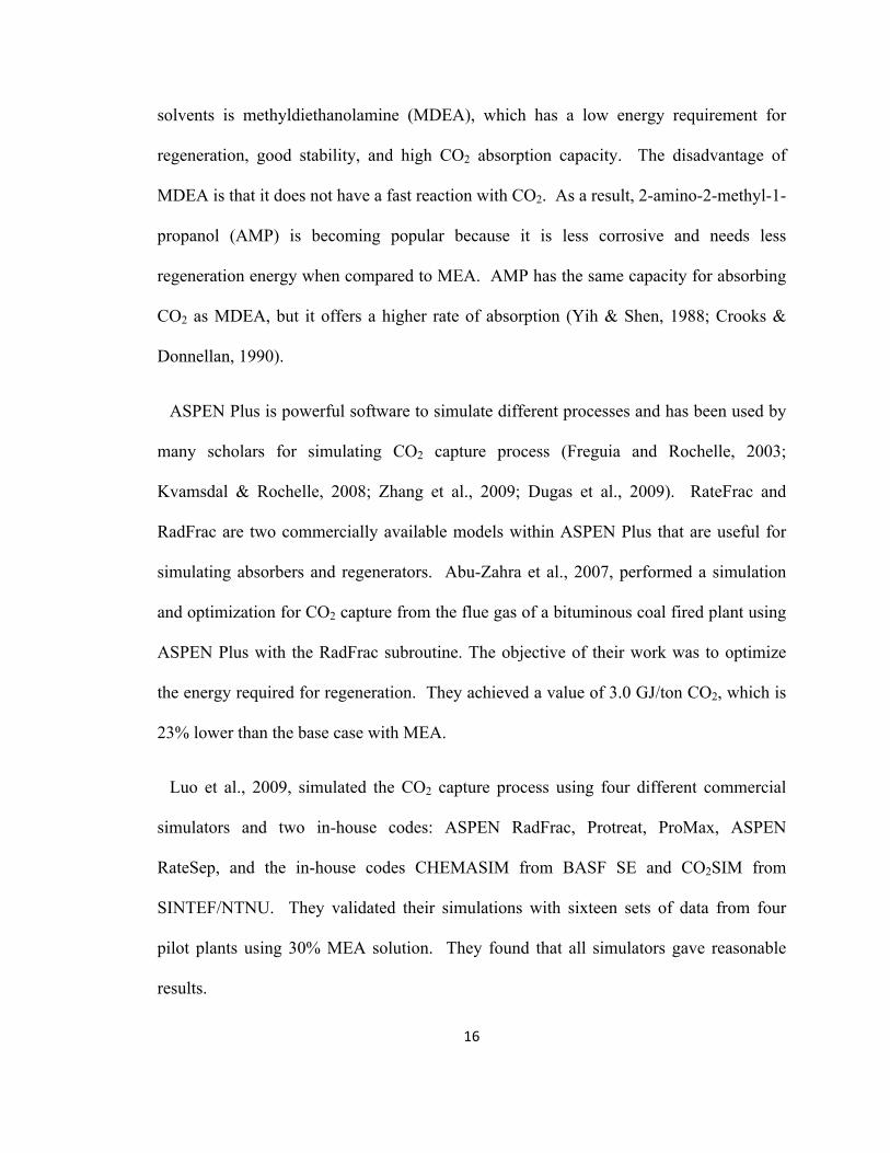
ASPEN Plus is powerful software to simulate different processes and has been used by
many scholars for simulating CO2 capture process (Freguia and Rochelle, 2003;
Kvamsdal & Rochelle, 2008; Zhang et al., 2009; Dugas et al., 2009). RateFrac and
RadFrac are two commercially available models within ASPEN Plus that are useful for
simulating absorbers and regenerators. Abu-Zahra et al., 2007, performed a simulation
and optimization for CO2 capture from the flue gas of a bituminous coal fired plant using
ASPEN Plus with the RadFrac subroutine. The objective of their work was to optimize
the energy required for regeneration. They achieved a value of 3.0 GJ/ton CO2, which is
23% lower than the base case with MEA.
Luo et al., 2009, simulated the CO2 capture process using four different commercial
simulators and two in-house codes: ASPEN RadFrac, Protreat, ProMax, ASPEN
RateSep, and the in-house codes CHEMASIM from BASF SE and CO2SIM from
SINTEF/NTNU. They validated their simulations with sixteen sets of data from four
pilot plants using 30% MEA solution. They found that all simulators gave reasonable
results.

17
Pellegrini et al., 2010, used a rate-based distillation model in ASPEN Plus to simulate a
CO2 capture plant. The energy requirement of two different process configurations, a
double column and a multi pressure column, were compared. For a given purification of
the solvent, operating pressure was the parameter that had the most significant effect on
the reboiler duty. The energy needed for stripping was much lower in the multi pressure
column configuration than that in the double column configuration.
Simulators without a proper mathematical model cannot give reasonable predictions.
Unfortunately, there are not very many mathematical models describing CO2 absorption
in amines in the literature. Some thermodynamic models have been developed for
predicting experimental data. The models proposed by Kent & Eisenberg, 1976, and
Chen et al., 1979, are the most famous. The last one is referred to as the Electrolyte-
NRTL and is based on the excess Gibbs free energy of the mixture. This model can be
used under a wide range of temperatures and loadings. Hilliard, 2008, has used
Electrolyte-NRTL to develop a new thermodynamic model describing amine systems
behavior. His model is more accurate than previous models. Plaza et al., 2009, used
Hilliard’s model and kinetics extracted from values obtained by Aboudheir, 2002, to
propose a new MEA model that was solved using ASPEN Plus. The results from their
simulation have been validated with pilot plant data.
2.6 Worldwide Research Centers and Pilot Plants for CO2 Capture
Wang et al., 2010, compiled the following list of research centres and CO2 capture pilot
plants from around the world that are trying to address this problem:

18
1. Luminant Carbon Management Programme (University of Texas at Austin)
2. International Test Centre for CO2 Capture (University of Regina)
3. CASTOR (EU Countries)
4. iCap (European Commission)
5. CAPRICE (International Research Project)
6. CESAR (International Research Project)
7. NZEC Initiative (UK and China)
8. CO2CRC (Australia and New Zealand)
9. Mitsubishi Heavy Industries R&D (Japan)
2.7 Integration of Power Plant with Post-Combustion CO2 Capture Plant
Aroonwilas and Veawab, 2007, simulated the capture of CO2 from a 500 MW
supercritical coal fire plant using MEA, MDEA and a mixture of both. They decreased
the regeneration heat requirement with a specific mixture of MEA and MDEA and
improved the efficiency of the whole power plant and CO2 capture plant by 3% when
compared to just using MEA. CO2 capture from pulverized coal power plant with MEA
has also been investigated by Chalmers & Gibbins, 2007, who recommended further
detailed study in a number of scenarios related to system operation. Kvamsdal et al.,
2010, studied the effect of integrating CO2 capture with MEA in a 450 MW natural gas
combined cycle (NGCC). They found that a 9% decrease in efficiency would happen for
plants that operate at 90% CO2 recovery and CO2 compression to 12 MPa.
The three studies mentioned above have all been for steady state conditions. Recently
Lawal et al., 2010, developed a dynamic model for CO2 capture using chemical

19
absorption. They used the developed model for investigating an integrated enhanced-O2
coal-fired power plant with CO2 capture (Lawal et al., 2011a). The results show that the
higher CO2 partial pressure, the lower required heat for regeneration. Through four case
studies, Lawal et al., 2011b, performed a scale-up for post-combustion CO2 capture
integrated with a 500 MW subcritical power plant and studied the effect of different
parameters on the performance of the system.
Romeo et al., 2008, introduced some solutions for decreasing the reboiler duty by
retrofitting a CO2 capture plant with a power plant. They also completed an economical
assessment and technical analysis in their paper. The main idea in their work is to use
different energy sources to meet the energy requirements of the reboiler in order to
decrease the cost of CO2 capture. For example, they suggest that when adding CO2
capture to a power plant, the steam or gas turbine could provide energy to the reboiler
while at the same time provide energy for CO2 compression. In this scenario, steam has
to be extracted from the turbines in a way that optimizes the performance and efficiency
of the power plant.
2.8 Economic Evaluation of Power Plant Integrated with CO2 Capture Plant and
CO2 Enhanced Oil Recovery
There have been a few research projects on the economic evaluation of CO2 capture
plant in the literature. deMontigny et al. (1997) investigated the possibility of reducing the cost
of CO2 production for EOR using cogeneration concepts. They studied natural gas power plants
with different capacities integrated with CO2 capture plants, but they concluded that the market
for oil and electricity at the time make the project economically unfeasible.

20
Tontiwachwuthikul et al. (1998) studied the technical and economic feasibility of
capturing CO2 from a coal-fired power plant to use the CO2 for EOR in Saskatchewan.
They used cogeneration concepts and optimization strategies to reduce the cost of CO2
capture. They concluded that the project is technically feasible and cogeneration and
optimization strategies can decrease expenses significantly, but capital and operating
expenses for capturing CO2 was too high for the oil market at the time.

21
2.8 Objective
The objective of this thesis is to study the economic feasibility of capturing CO2 from a
combined cycle power plant with the nominal capacity of 500 MW and compressing it to
use for EOR as an integrated system. The typical size of natural gas combined cycle
power plants offered by Alstom, General Electric and Siemens, three major
manufactures, ranges from 50 MW to 500 MW. Cost of the plant depends on the size, but
larger plants take advantage of economy of scale, which lowers the cost per kilowatt of
produced electricity.
In order to estimate the cost of purchased equipment, a simulation was done for the
power plant, CO2 capture plant, and CO2 compression plant. The data from the simulation
was used to size the major equipment and estimate the capital and operating cost of the
project. Using capital and operating costs, the profitability of the project was calculated
with respect to the return on investment, payback period, net return, net present worth,
and discounted cash flow rate of return. The effect of the price of natural gas, oil,
electricity, and oil production to injected CO2 ratio has been examined for its effect on
the profitability of the project.

22
CHAPTER 3: METHODOLOGY
The aim of this thesis is to perform a cost estimation and economic evaluation on CO2
capture from a 500 MW natural gas combined cycle power plant for injection into an oil
reservoir for enhanced oil recovery (EOR). This integrated system was evaluated
economically using 2012 costing figures. The operating conditions for the power plant
were adopted from the U.S. Department of Energy (U.S. DOE) & National Energy
Technology Laboratory (NETL) (2011).
Post-combustion CO2 capture with MEA solutions was selected as the separation
technology. The operating conditions for CO2 capture plant were the typical conditions
found in the literature.
It has been considered that the main part of the cost for injecting CO2 into a reservoir is
the cost of the compression unit. Therefore, other EOR expenses such as CO2 injection
well components have been neglected compare to the cost of CO2 compression unit.
Also, in this study, CO2 recycle for enhanced oil recovery has not been considered
because of the complexity of the process. Such a considering would increase the capital
cost and payback period of the project.
Cost estimation and economic evaluation is the backbone of this thesis. According to
the information and the time available for the purpose of this thesis, the accuracy of the
method that has been used is ±20%. All the procedures and methods for cost estimation
and economic evaluation are from Peters et al. (2003). The capital cost has been

23
estimated using a percentage of delivered-equipment cost method that will be explained
in detail later in section 3.2.
In order to estimate the cost of purchased equipment, the major equipment components
needed to be sized. Material balance tables for all units were obtained through the
simulations. In this study, Aspentech Hysys was used for process simulation. The results
were presented as material balance tables for each unit. The data from the material
balance tables were then used with the Peters et al. (2003) online cost estimator to
determine equipment costs. When equipment was not available in this online cost
estimator, equipment prices from Fisher et al. (2005) and the U.S. DOE & NETL (2011)
were used. Modifications for the capacities required in this project were determined by
applying the six-tenths factor rule from Peters et al. (2003). There are a number of
exponential factors for different types of equipment that can be used instead of 0.6, but
all of those factors are less than 0.6 for the equipment sized in this study. The estimated
capital cost of major equipment is slightly higher when using the six-tenth rule instead of
different exponential factors for each equipment. All the prices from different years have
been converted to 2012 prices using chemical engineering plant cost indexes that are
published each month in Chemical Engineering.

24
3.1 Simulation
3.1.1 Natural Gas Combined Cycle Power Plant
3.1.1.1 Process Description
A simplified natural gas combined cycle (NGCC) power plant configuration from the
U.S. DOE & NETL (2011) has been used in this study. The design is based on two
advanced F class combustion turbine generators (CTG), two heat recovery steam
generator (HRSG) systems, and one steam turbine generator (STG) that are considered to
be commercially available. However, in the process flow diagram that can be seen in
Figure 3.1, only one CTG and HRSG have been displayed. However, in the material
balance table (Table A.1, A.2, A.3, and A.4), the flow rates are for two trains. It was
considered that natural gas (NG) is available in the battery limit of the plant at 3 MPa and
38 °C, which is compatible with the requirements of advanced F class CTGs. The flow
rate of NG into the power plant depends on the capacity of the CTG system. CTGs are
available in discrete sizes and STCs are available in wide range of capacities. The amount
of sulfur compounds in the natural gas stream is assumed negligible. Therefore, the
emission of SOx can be neglected. To control the emission of NOx, a low NOx burner and
selective catalytic reduction technology was applied to reduce the emission of NOx to 2.5
ppmv at 15% O2. The NOx control system is assumed to be included in HRSG and the
details of the system are out of the scope of this study. Also, natural gas is assumed to
contain no mercury and particulate matters, therefore, no control is required for mercury
and particulate matters.

25
The nominal net plant electricity production for this study is 500 MW but the actual
electricity production changes because of the requirements of the CO2 capture and
compression plant. The CTG system consists of an air compressor, combustor and gas
turbine. Air, at atmospheric pressure and 25 °C, enters the air compressor and is
compressed to 3 MPa. NG mixes with compressed air in the combustor and it is assumed
that combustion is complete and all the carbons in NG convert to CO2. Combustion gas
produces electricity in gas turbine and the flue gas leaves the gas turbine at atmospheric
pressure and 671 °C. The flue gas enters to HRSG in order to produce steam for a single
reheat 16.5 MPa/566 °C steam cycle. The flue gas leaves the HRSG at 90 kPa and 142 °C
and goes to the CO2 capture unit as the feed. The steam required for the CO2 capture unit
stripper reboiler is extracted from steam cycle at 446.1 kPa and 281 °C as saturated steam
and returns as saturated water at the same conditions. The steam cycle consists of a
HRSG, STG, condenser, and condensate pump to form a Rankine cycle for electricity
production.

26
Figure 3.1: Natural gas combined cycle power plant process flow sheet

27
3.1.1.2 Key Process Simulation Specifications
The fluid package used for the simulation of the power plant is Soave-Redlich-Kwong
(SRK). A summary of simulation inputs is displayed in Table 3.1. From this table, the
temperature and pressure of the natural gas is 38 °C and 3100 kPa, respectively, which is
compatible with advanced F class gas turbines (U.S. DOE & NETL, 2011). Air is
considered to enter at standard condition and compress up to 3100 kPa to mix with
natural gas in the combustor. Saturated steam at 466.1 kPa goes to the CO2 capture plant
reboiler and returns to the steam cycle as saturated water at 466.1 kPa. The data in Table
3.1 comes from studies done by the U.S. DOE & NETL (2011).

28
Table 3.1: Natural gas combined cycle power plant key process simulation specifications
Natural Gas
Temperature (°C) 38.00 Pressure (kPa) 3,100.00
Molar Flow (kmol/h) 4,020 Composition (mole fraction) -
C1 0.93 C2 0.03 C3 0.01 C4 0.00
CO2 0.01 H2O 0.00 O2 0.02 N2 0.00
Air
Temperature (°C) 25.00 Pressure (kPa) 101.32
Molar Flow (kmol/h) 98174 Composition (mole fraction) -
O2 0.79 N2 0.21
Air Compressor Outlet Pressure (kPa) 3,100.00 Combustor Conversion Reactor with 100% Conversion
Gas Turbine Outlet Pressure (kPa) 101.32 Efficiency 85%
Flue Gas Temperature (°C) 142.00 Pressure (kPa) 90.00
HP Steam Temperature (°C) 566.00 Pressure (kPa) 16,500.00
Steam Turbine Outlet Pressure (kPa) 5 Efficiency 75%
Condenser Outlet Temperature (°C) 31 Condensate Pump Discharge Pressure (kPa) 16,500.00
Efficiency 65%
Steam to Reboiler Vapor Fraction 1
Temperature (°C) 149.35 Pressure (kPa) 466.10
Steam from Reboiler Vapor Fraction 0

29
3.1.2 CO2 Capture Unit
3.1.2.1 Process Description
The CO2 capture unit in this thesis is based on the Fluor Econamine FG PlusSM
technology (Sander & Maritz, 1992) that is suitable for recovering CO2 from low
pressure stream with the presence of O2 such as flue gas stream from fossil fuel power
plants. The process flow diagram of CO2 capture unit is displayed in Figure 3.2.

30
Figure 3.2: CO2 capture plant process flow sheet

31
The CO2 capture plant was been designed to remove 90% of the CO2 from flue gas
stream coming from the power plant. The flue gas goes through the flue gas cooler to
cool down to 39 °C. Then, it goes to a separator to separate the condensed water from
previous step. The condensed water is used as cooling tower makeup water and the flue
gas goes to the flue gas blower. The flue gas blower increases the pressure and
temperature of the flue gas to 111.32 kPa and 50 °C that is appropriate for the absorber.
The flue gas enters the bottom of the absorber and the lean MEA (30 wt.%) with a CO2
loading of 0.2 mole CO2/mole MEA enters from the top of the column at atmospheric
pressure and 40 °C. The typical number of stages for an absorber is about 20 for tray
column, or the length of packing equivalent to 20 stages for a packed column. In many
cases, the length or number of stages in an absorber is selected from previous plants
(Kohl & Nielsen, 1997). The number of stages for the absorber in this study is 27 to
achieve a rich amine CO2 loading of 0.4 mole CO2/mole MEA and 90% CO2 recovery.
Exhaust gas from the top of the absorber goes to the water wash section to recover 80%
of the amine remaining in the exhaust gas. There are 7 stages needed in the wash water
column to recover 80% of the amine. The treated gas leaves the water wash column from
the top. Roughly 5% of the liquid from the bottom returns to the absorber and the rest
recycles to the wash water column through a pump and cooler where wash water makeup
is added to it. The rich amine from the bottom of the absorber goes to the rich amine
pump to increase the pressure to 482.40 kPa. Then, it goes to a lean/rich amine heat
exchanger with a temperature approach of 10 °C to warm up the rich amine to 110 °C.
Rich amine enters the stripper from the top. The typical number of stages for a stripper is
12 to 20. In this study the stripper has 13 stages. The CO2 stream leaves the condenser

32
with a purity of 97 mole% and goes to the compression unit. The reboiler operates at 120
°C in the bottom of the stripper to regenerate the MEA solution. Based on the simulation
results, 6.1 GJ heat is required in the reboiler per tonne of produced CO2. The CO2
loading of the lean amine from the reboiler is 0.2 mole CO2/mole MEA. The lean amine
goes to a lean amine pump where the pressure is increased up to 447.90 kPa. After the
pressure increase, it goes to a lean/rich amine heat exchanger for an initial cool down,
and then to the lean amine cooler to cool all the way down to 40 °C. Before the lean
amine cooler, makeup amine is injected to the amine stream. After cooling down, amine
enters the absorber from the top to complete the amine cycle.
3.1.2.2 Key Process Simulation Specifications
The fluid package used for the simulation of the CO2 capture unit is Aspen Hysys
Amine Package. A summary of simulation inputs is displayed in Table 3.2a, b. The outlet
temperature of the flue gas cooler is 39 °C, which is lower than the temperature of the
flue gas entering the absorber. This is because of the increase in the flue gas temperature
through the flue gas blower. For a 90% CO2 recovery, rich amine loading of 0.4 mole
CO2/mole MEA, and liquid flow rate of 160000 mol/h, the absorber will have 27 stages.
The wash water makeup has been calculated to recover 80% of the amine (Kohl &
Nielsen, 1997).

33
Table 3.2a: CO2 capture plant key process simulation specifications
Flue Gas
Temperature (°C) 142.00 Pressure (kPa) 101.32 Molar Flow (kmol/h) 102,310.5
8 Composition (mole fraction) - CO2 4.09E-02 H2O 7.88E-02 MEA 0.00E+00 O2 1.22E-01 N2 7.59E-01
Flue Gas Cooler Outlet Temperature (°C) 39.00 Flue Gas Blower Outlet Pressure (kPa) 111.30
Lean Amine
Temperature (°C) 40.00 Pressure (kPa) 101.32 Molar Flow (kmol/h) 160,000 Composition (mole fraction) - CO2 2.32E-02 H2O 8.61E-01 MEA 1.16E-01 O2 7.50E-58 N2 4.78E-60
Absorber
Number of Stages 27 Top Pressure (kPa) 101.32 Bottom Pressure (kPa) 107.85 CO2 Removal 90% Rich Amine CO2 Loading(mole CO2/mole MEA) 0.4
Water Wash Section
Number of Stages 7 Top Pressure (kPa) 101.32 Bottom Pressure (kPa) Amine Recovery 80%
Wash Water Stream Splitter
Split Ratio 19:1 Wash Water Pump Outlet Pressure (kPa) 101.32
Wash Water Makeup
Temperature (°C) 25.00 Pressure (kPa) 101.32 Molar Flow (kmol/h) 999.16 Composition (mole fraction) - H2O 1.00E+00
Wash Water Cooler Outlet Temperature (°C) 37.50

34
Table 3.2b: CO2 capture plant key process simulation specifications Rich Amine Pump Outlet Pressure (kPa) 482.40
Rich/Lean HEX Hot Side Outlet Temperature (°C) 110.00 Cold Side Outlet Temperature (°C) 55.75 Temperature Approach (°C) 10
Stripper
Number of Stages 13 Top Pressure (kPa) 181.30 Bottom Pressure (kPa) 189.90 Reboiler Temperature (°C) 120.00 CO2 Mole Fraction in CO2 Product 0.97 Lean Amine CO2 Loading (mole CO2/mole MEA) 0.2
Lean Amine Pump Outlet Pressure (kPa) 447.90
MEA Makeup
Temperature (°C) 25.00 Pressure (kPa) 101.32 Molar Flow (kmol/h) 8.32 Composition (mole fraction) - MEA 1.00E+00
Water Makeup
Temperature (°C) 25.00 Pressure (kPa) 101.32 Molar Flow (kmol/h) 3,462.54 Composition (mole fraction) - H2O 1.00E+00
Lean Amine Cooler Outlet Temperature (°C) 40.00

35
3.1.3 CO2 Compression Unit
3.1.3.1 Process Description
In order to provide CO2 for EOR injection, the pressure must increase up to around 14.7
MPa, which is a typical pressure for EOR. The number of compression stages is based on
a maximum temperature of 177 °C and a maximum compression ratio of 3. The
condensed water from the interstage separators was used as cooling tower makeup water.
Figure 3.3 shows the process flow sheet of the CO2 compression plant.

36
Figure 3.3: CO2 compression plant process flow sheet

37
3.1.3.2 Key Process Simulation Specifications
The fluid package used for the simulation of the CO2 compression unit is SRK. A
summary of simulation inputs is displayed in Table 3.3.
Table 3.3: CO2 compression plant key process specifications
CO2 Product
Temperature (°C) 34.02 Pressure (kPa) 181.30 Molar Flow (kmol/h) 3,904.11 Composition (mole fraction) - CO2 9.70E-01 H2O 2.96E-02 MEA 0.00E+00 O2 8.98E-05 N2 2.97E-04
K-200 Compression Ratio 3 Efficiency (polytropic) 79.5%
E-200 Outlet Temperature (°C) 40.00
K-201 Compression Ratio 3 Efficiency (polytropic) 79.5%
E-201 Outlet Temperature (°C) 40.00
K-202 Compression Ratio 3 Efficiency (polytropic) 79.5%
E-202 Outlet Temperature (°C) 40.00
K-203 Compression Ratio 3 Efficiency (polytropic) 79.5%
E-203 Outlet Temperature (°C) 40.00

38
3.2 Capital Cost Estimation
The sum of money needed before putting an industrial plant into operation to buy all of
the equipment, piping, controls, and service facilities is called capital cost. Capital cost is
classified as fixed-capital investment and working capital. Fixed-capital investment refers
to the capital needed to build the plant and working capital is money required for
operating the plant. The sum of fixed-capital investment and working capital is called
total capital investment. Fixed-capital investment is divided into manufacturing fixed-
capital investment, or direct cost, and nonmanufacturing fixed-capital investment, or
indirect cost. The components of fixed-capital investment are as follows:
• Direct costs:
1. Purchased equipment
2. Purchased equipment delivery
3. Purchased equipment installation
4. Instrumentation and controls
5. Piping
6. Electrical systems
7. Buildings (including services)
8. Yard improvements
9. Service facilities
10. Land
• Indirect costs:
1. Engineering and supervision

39
2. Construction expenses
3. Legal expenses
4. Contractor’s fee
5. Contingency
The components of working capital are listed below:
1. Raw materials and supplies carried in stock
2. Finished products in stock and semi finished products in the process of being
manufactured
3. Accounts receivable
4. Cash kept on hand for monthly payment of operating expenses, such as salaries,
wages, and raw material purchases
5. Accounts payable
6. Taxes payable
There are various methods for capital cost estimation. Choosing a specific method
depends on detail information available and desired accuracy. Capital cost estimation
methods are:
1. Detailed-item estimate
2. Unit cost estimate
3. Percentage of delivered-equipment cost
4. Lang factors for approximation of capital investment
5. Power factor applied to plant/capacity ratio

40
6. Invest cost per unit of capacity
7. Turnover ratio
The details of each method can be found in (Peters et al., 2003). For the purposes of this
study, and based on the detail information available, the percentage of delivered-
equipment cost method has been used. In this method, the cost of major equipment is
estimated from the literature, existing plants with similar configuration, and vendors. The
cost of delivering the equipment is represented as a percentage of the purchased
equipment cost. Other components of capital cost are calculated as a percentage of the
delivered-equipment cost. The accuracy of this method is in the range of ±20 to 30
percent. The more equipment that is included in the major equipment list, the more
accurate this method becomes. Therefore, as a first step, a detailed major equipment list
needs to be prepared.
3.2.1 Major Equipment List
Major equipment is listed in 3.4 for different units. There is minor equipment that has
not been considered in this research. This minor equipment is neglected because its cost
and importance are less than that of major equipment. Minor equipment includes the
amine surge tank, amine storage tank, makeup amine pump, water storage tank, and
makeup water pump.

41
Table 3.4: Major equipment list
Power Plant
Gas Turbine HRSG Steam Turbine Condenser Condensate Pump
CO2 Capture Unit
Flue Gas Cooler Flue Gas Blower KO Drum Flue Gas Blower Absorber Water Wash Wash Water Pump Wash Water Cooler Rich Amine Pump Rich/Lean Heat Exchanger Stripper Reboiler Condenser Reflux Accumulator Reflux Pump Lean Amine Pump Lean Amine Cooler Packing Filter Reclaimer
CO2 Compression Unit Iterstage Coolers Interstage Separators CO2 Compressors

42
3.2.2 Major Equipment Sizing and Purchase Cost
To estimate the equipment cost, the quantity of equipment, type of equipment, material
of construction, and size of equipment is needed. Spare equipment has been considered
for all mechanical equipment such as pumps and compressors, and the type and material
of construction have been determined from the literature. For calculating the cost, a
parameter that represents the size of the equipment is required. Size parameters are
calculated from the data in material balance table and data from the simulations. The cost
estimation for equipment that used size parameters that were out of the range of online
cost estimator, or were different than the size in the literature, the six-tenth rule from
Peters et al., 2003 has been used as Equation 3.1:
Cost of equipment a = cost of equipment b × !"#"!$%& !" !"#$%&!'( !!"#"!$%& !" !"#$%&!'( !
!.! (3.1)
For most of the equipment, the cost has been estimated from Peters et al. (2003) online
cost estimator and the cost of the other equipment has been found from the literature for
the same equipment with similar configuration. The cost from online cost estimator and
the literature are for year 2002, 2004, and 2007. In order to convert the cost for year
2012, chemical engineering plant indexes for each equipment has been used through the
Equation 3.2 (Peters et al., 2003),
Present cost = original cost !"#$% !"#$% !" !"#$#%&!"#$% !"#$% !" !"#$ !"#$#%&' !"#$ !"# !"#$%&'(
(3.2)
Chemical engineering plant indexes for year 2002, 2004, 2007, and 2012 are 390.4,
444.2, 525.4, and 593.8 (Lozowski, 2007; Lozowski, 2012) respectively.

43
The size parameter for the absorber, stripper and wash water column is weight. For
calculating the weight of these columns, column length and diameter are required.
Diameter of packed columns can be calculated from the pressure drop correlation
displayed in Figure 3.4. Length, or height of the column, can be estimated by the number
of ideal stages times HETP. Y-axis in this graph is called flow capacity factor and X-axis
is called relative flow capacity. The results of column sizing have been summarized in
Table 3.5.

44
Figure 3.4: Pressure drop correlation for packed towers (Kohl & Nielson, 1997)

45
Table 3.5: Summary of column sizing Parameter Absorber Stripper Wash Water Unit
L 4,163,580 4,279,080 554,980 lb/h
G 3,177,395 533,325 3,090,108 lb/h
Liquid kinematic viscosity 1.45 0.39 0.80 cSt
Gas density 0.07 0.07 0.06 lb/ft^3 Liquid density 64.00 63.18 64.78 lb/ft^3
F 18 18 18 -
ΔP 0.47 0.47 0.47 in water/ft Relative flow capacity 0.04 0.27 0.01 -
Flow capacity factor 0.06 0.03 0.07 -
G* 0.70 0.48 0.73 lb/ft^2s
A 1,264.48 311.85 1,175.16 ft^2 D 40.12 19.93 38.68 ft
D 12.23 6.07 11.79 m
HETP 0.76 0.76 0.76 m Number of stages 27 13 7 -
Length 20.47 9.85 5.31 m
Wall thickness 0.01 0.01 0.01 m Volume of shell + heads 10.23 2.47 4.16 m^3
Density of CS 7,850 7,850 7,850 kg/m^3
Weight of shell + heads 80,282 19,362 32,640 kg
Volume of packing 2,404.23 285.49 579.29 m^3 Bulk weight of packing 166 166 166 kg/m^3
Weight of packing 399,103 47,391 96,162 kg

46
The size parameter for heat exchangers, condensers, and coolers is area. Area (m2) of
the heat exchangers is calculated from Equation 3.3 and 3.4 (GPSA, 2004),
A = !!×!"#$
(3.3)
LMTD = !!,!!!!,! ! !!,!!!!,!
!" !!,!!!!,!!!,!!!!,!
(3.4)
Heat transfer coefficients (U) are listed in Table 3.6 for different systems. Other
parameters can be found from material balance tables and simulations.
The size parameter for compressors is the required power (kW) that can be extracted
from the simulations.
The size parameter for pumps is volumetric flow rate (m3/s)×discharge pressure (kPa)
that can be easily calculated from material balance tables and the simulations.
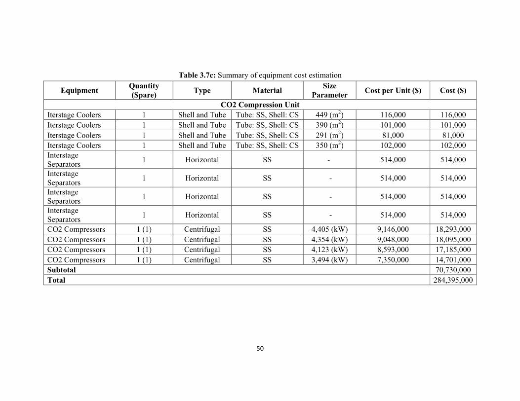
The results of the cost estimation are listed in Table 3.7a, b, c.

47
Table 3.6: Overal heat transfer coefficients in tubular heat exchangers (GPSA, 2004; Perry, 1997)
Shell Side Tube Side Overal Heat Transfer Coefficient (Btu/°F.ft2.h) Water Air, N2 20-40 Water Water 180-200 MEA MEA 120-130 Water Amine 100-110 Steam Water 400-1000 Water 100 psia Gas 35-40 Water 300 psia Gas 40-50 Water 700 psia Gas 60-70 Water 1000 psia Gas 80-100
Note: 1 Btu/°F.ft2.h = 5.678 J/°C.m2.h

48
Table 3.7a: Summary of equipment cost estimation
Equipment Quantity (Spare) Type Material Size Parameter Cost per
Unit ($) Cost ($)
Power Plant
Gas Turbine 2 170 MW advanced F class w/dry low-NOx burner - - 42,549,000 85,097,000
HRSG 2 Drum, multi-pressure with
economizer section and integral dearator
- - 27,646,000 55,292,000
Steam Turbine 1 Tendem compound, HP, IP, and tow-flow LP turbine - - 20,257,000 20,257,000
Condenser 1 Shell and Tube Tube: SS, Shell: CS 2744 (m2) 318,000 318,000
Condensate Pump 1 Centrifugal CS 900 (m3.kPa/s) 314,000 314,000
Subtotal 161,278,000

49
Table 3.7b: Summary of equipment cost estimation
Equipment Quantity (Spare) Type Material Size Parameter Cost per
Unit ($) Cost ($)
CO2 Capture Unit Flue Gas Cooler 1 Shell and Tube Tube: SS, Shell: CS 8,857 (m2) 642,000 642,000 Flue Gas Blower KO Drum 1 Horizontal SS - 5,210,000 5,210,000 Flue Gas Blower 1 (1) Forced Draft SS 2,882,514 (kW) 1,714,000 3,428,000 Absorber 2 Packed Shell: CS, Packing: SS 80,282 (kg) 609,000 1,219,000 Water Wash 2 Packed Shell: CS, Packing: SS 32,640 (kg) 248,000 495,000 Wash Water Pump 1 (1) Centrifugal SS 13 (m3.kPa/s) 16,000 31,000 Wash Water Cooler 1 Shell and Tube Tube: SS, Shell: CS 284 (m2) 74,000 74,000 Rich Amine Pump 1 (1) Centrifugal SS 497 (m3.kPa/s) 220,000 440,000 Rich/Lean Heat Exchanger 1 Shell and Tube Tube: SS, Shell: CS 35,271 (m2) 1,470,000 1,470,000 Stripper 2 Packed Shell: CS, Packing: SS 19,362 (kg) 147,000 294,000 Reboiler 2 Kettle Type Tube: SS, Shell: CS - 1,673,000 3,347,000 Condenser 2 Shell and Tube Tube: SS, Shell: CS 3,295 (m2) 355,000 709,000 Reflux Accumulator 2 Horizontal SS - 18,000 36,000 Reflux Pump 2 (2) Centrifugal SS 6 (m3.kPa/s) 13,000 53,000 Lean Amine Pump 1 (1) Centrifugal SS 471 (m3.kPa/s) 213,000 425,000 Lean Amine Cooler 1 Shell and Tube CS 2,962.70 (m2) 333,000 333,000
Packing 2 IMTP50 SS 2,404+ 579+285 (m3) 16,302,000 32,604,000
Filter 1 Horizontal CS - 503,000 503,000
Reclaimer 1 Horizontal-Kettle Tube: SS, Shell: CS - 1,074,000 1,074,000
Subtotal 52,387,000
50
Table 3.7c: Summary of equipment cost estimation
Equipment Quantity (Spare) Type Material Size
Parameter Cost per Unit ($) Cost ($)
CO2 Compression Unit Iterstage Coolers 1 Shell and Tube Tube: SS, Shell: CS 449 (m2) 116,000 116,000 Iterstage Coolers 1 Shell and Tube Tube: SS, Shell: CS 390 (m2) 101,000 101,000 Iterstage Coolers 1 Shell and Tube Tube: SS, Shell: CS 291 (m2) 81,000 81,000 Iterstage Coolers 1 Shell and Tube Tube: SS, Shell: CS 350 (m2) 102,000 102,000 Interstage Separators 1 Horizontal SS - 514,000 514,000
Interstage Separators 1 Horizontal SS - 514,000 514,000
Interstage Separators 1 Horizontal SS - 514,000 514,000
Interstage Separators 1 Horizontal SS - 514,000 514,000
CO2 Compressors 1 (1) Centrifugal SS 4,405 (kW) 9,146,000 18,293,000 CO2 Compressors 1 (1) Centrifugal SS 4,354 (kW) 9,048,000 18,095,000 CO2 Compressors 1 (1) Centrifugal SS 4,123 (kW) 8,593,000 17,185,000 CO2 Compressors 1 (1) Centrifugal SS 3,494 (kW) 7,350,000 14,701,000 Subtotal 70,730,000 Total 284,395,000

51
3.2.3 Total Capital Investment
Total capital investment and its components for this project can be seen in Table 3.8.
Table 3.8: Total capital cost components
Capital Cost Components Fraction of delivered equipment Calculated values, million $
Direct Costs Purchased equipment, E - 284.40 Delivery, fraction of E 0.10 28.44 Subtotal: delivered equipment - 312.83
Purchased equipment installation 0.47 147.03
Instrumentation & Controls (installed) 0.36 112.62
Piping (installed) 0.68 212.73 Electrical systems (installed) 0.11 34.41
Buildings (including services) 0.18 56.31
Yard improvements 0.10 31.28 Service facilities (installed) 0.70 218.98 Total direct costs 2.60 1126.20
Indirect Costs Engineering and supervision 0.33 103.24 Construction expenses 0.41 128.26 Legal expenses 0.04 12.51 Contractor's fee 0.22 68.82 Contingency 0.44 137.65 Total indirect costs 1.44 450.48
Fixed capital investment (FCI) 1576.69 Land 0.06 17.06
Working capital (WC) 0.89 278.42 Total capital investment (TCI) 1855.11

52
3.3 Operating Cost Estimation
Total operating cost includes all expenses such as costs for producing the products,
selling the products, and recovering of capital cost. The total operating cost is classified
as manufacturing costs and general expenses. Manufacturing costs are all expenses
related to production. Manufacturing cost is also called operating or production cost.
Manufacturing cost categorizes into three subdivisions: 1) variable production costs, 2)
fixed charges, and 3) plant overhead costs. The components of total production cost are
listed below:
• Manufacturing cost
o Variable cost
§ Raw materials
§ Operating labor
§ Operating supervision
§ Utilities
§ Maintenance and repairs
§ Operating supplies
§ Laboratory charges
§ Royalties
§ Catalysts and solvents
o Fixed charges
§ Taxes (property)
§ Financing (interest)

53
§ Insurance
§ Rent
§ Depreciation
o Plant overhead
• General expenses
o Administration
o Distribution and selling
o Research and Development
Utility consumption, raw materials and products costs, and the required operating labor
needs to be calculated. The other components of total production cost are calculated as a
percentage of these parameters and fixed capital investment, as per the procedure
outlined by Peters et al., 2003.
3.3.1 Utility Consumption
Utilities include electricity, fuel, refrigeration, steam, water treatment and disposal,
process water, and cooling water.
The electricity for all of the equipment has been provided by the power plant. The
steam required for the stripper reboiler in the CO2 capture plant is produced from the
power plant steam cycle. No refrigeration or water treatment and disposal system has
been considered in this study. The information require for calculating the required utility
is from the simulations. The utility consumption of each plant has been listed in Table
3.9a, b.

54
Table 3.9a: Utility consumption summary Electricity
Item Duty (kW) Power Plant
Air Compressor 484,617 Gas Turbine -825,888 Steam Turbine -60,942 Condensate Pump 1,389 Subtotal -400,824
CO2 Capture Unit Flue Gas Blower 9,087 Rich Amine Pump 594 Lean Amine Pump 417 Wash Water Pump 0 Subtotal 10,098
CO2 Compression Unit K-200 4,405 K-201 4,354 K-203 4,123 K-204 3,494 Subtotal 16,375 Total -374,351
Coolers Duty Item Duty (kW)
Power Plant Condenser 123,715 Subtotal 123,715
CO2 Capture Unit Lean Amine Cooler 59,087 Wash Water Cooler 6,265 Flue Gas Cooler 100,559 Condenser 169,571 Subtotal 335,482
CO2 Compression Unit E-200 5,032 E-201 5,225 E-203 5,933 E-204 11,900 Subtotal 28,090 Total 487,287

55
Table 3.9b: Utility consumption summary Cooling Water (15 C - 30 C)
Item Flow (kg/h) Power Plant 6,688,774 CO2 Capture Unit 18,138,089 CO2 Compression Unit 1,518,702 Total 26,345,565
Reboilers Duty Item Duty (kW)
CO2 Capture Unit Reboiler 287,927 Total 287,927
Steam (466.1 kPa) Item Flow (kg/h)
CO2 Capture Unit 287,927 Total 287,927
Process Water Item Flow (kg/h)
CO2 Capture Unit Wash Water Makeup 18,000 Water Makeup 62,378 Stream 3 -19,478 Subtotal 60,900
CO2 Compression Unit Stream 2 -2 Stream 6 -1,089 Stream 10 -618 Stream 14 -165 Subtotal -1,874 Total 59,026
Fuel Item Flow (MMBtu/h)
Natural Gas 3118

56
Required cooling water has been calculated from the cooler duty using Equation 3.5:
m!""#$%& !"#$% =!"##×!!""#$%×(!!"#$% !" !" ℃!!!"#$% !" !" ℃)/!
!"!!" (3.5)
C!"#$% !" !" ℃ = 4435.5 (J/℃. kg); C!"#$% !" !" ℃ = 4442.6 (J/℃. kg)
The flow rate of steam can be calculated from the reboiler duty using Equation 3.6:
m!"#$% = !"##×!!"#$%&"!!!"#. !"#$% !" !"".! !"#
(3.6)
λ!"#. !"#$% !" !"".! !"# = 2137861 (J/kg)
The rest of amounts listed in Table 3.9a, b have been taken directly from the simulation.
The nominal capacity of the power plant is 500 MW but the actual capacity of the
power plant is less than nominal capacity because of the steam extracted for the reboiler
from the steam cycle of the power plant.
Annual utility consumption and the price per unit have been presented in Table 3.10.

57
Table 3.10: Annual utility consumption
Utility Unit Cost Annual Utility Requirement
Annual Utility Cost, million $/y
Fuel 2.09 $/MMBtu 27,314,381 MMBtu/y 57.09 Cooling Water 0.08 $/m3 114,307,651 m3/y 9.15 Process Water 0.53 $/m3 507,605 m3/y 0.27

58
3.3.2 Raw Materials and Products
The annual amount of raw materials and products, and the price per unit, has been
presented in Table 3.11.
Table 3.11: Annual amount of raw materials and products Raw Materials Unit Cost Annual Consumption Annual Cost, million $/y
MEA 1.95 $/kg 4.454 million kg/y 8.67
Products Unit Cost Annual Production Annual Cost, million $/y
Electricity 110 $/MWh 3.279 million MWh 360.73
Oil 100 $/barrel 4.842 million barrel/y 484.17

59
3.3.3 Labor
Using the data from Table 3.12, it is estimated that about 10 people are required to
operate the plant per shift. Assuming that there are 8 hours per shift, 3 shifts per day and
365 days per year, 876,00 employee-hours are needed annually. Average wage of
operating labor per hour is assumed to be 35 $. Therefore, 3.066 million $/y is the labor
cost for this project.

60
Table 3.12: Typical labor requirements for process equipments (Peters et al., 2003)
Type of Equipment Workers/Unit/Shift Number of Units Workers/Shift
Blowers and compressors 0.1-0.2 9 1.8 Centrifugal separator 0.25-0.50 - - Crystallizer, mechanical 0.16 - - Dryer, rotary 0.5 - - Dryer, spray 1.0 - - Dryer, tray 0.5 - - Evaporator 0.25 - - Filter, vacuum 0.125-0.25 - - Filter, plate and frame 1.0 1 1 Filter, rotary and belt 0.1 - - Heat exchangers 0.1 9 0.9 Process vessels, towers (including auxiliary pump and exchangers)
0.2-0.5 11 5.5
Reactor, batch 1.0 - - Reactor, continuous 0.5 - - Total 9.2

61
3.3.4 Total Product Cost Excluding Depreciation
Total production cost and its components for this project can be seen in Table 3.13.
Table 3.13: Total product cost components
Item Defau
lt factor
Basis
Basis cost,
million $/y
Cost, million
$/y
Raw materials - - - 8.67 Operating labor - - - 3.07 Operating supervision 0.15 of operating labor 3.07 0.46 Utilities - - - 66.50 Maintenance and repairs 0.06 of FCI 1619.60 97.17 Operating supplies 0.15 of maintenance & repair 97.18 14.58 Laboratory charges 0.15 of operating labor 3.07 0.46 Royalties (if not on lump-sum basis) 0.01 of co 355.62 3.56
Catalysts and solvents - - - 0.00 Variable cost = 194.47
Taxes (property) 0.02 of FCI 1619.60 32.39 Financing (interest) 0 of FCI 1619.60 0.00 Insurance 0.01 of FCI 1619.60 16.20 Rent 0 of FCI 1619.60 0.00 Depreciation Calculated separately
Fixed Charges = 48.59
Plant overhead, general 0.6 of labor, supervision and maintenance 100.70 60.42
Plant Overhead = 60.42 Manufacturing cost = 303.47
Administration 0.2 of labor, supervision and maintenance 100.70 20.14
Distribution & selling 0.05 of co 355.62 17.78 Research & Development 0.04 of co 355.62 14.22
General Expense = 52.15 TOTAL PRODUCT COST WITHOUT DEPRECIATION = co = 355.62

62
3.3.5 Depreciation
Depreciation is included in the total product cost under the fixed charges group. The
idea behind depreciation is that the value of the physical equipment decreases with time.
Additionally, depreciation must be deducted from income for calculating the income tax.
Therefore, depreciation must be considered in the total product costs.
There are various methods for calculating depreciation. The method that has been used
in this study is the declining balance (DB) method. In this method, a fixed fraction is
selected as the rate of depreciation for the depreciable capital each year. For this project,
0.1 has been selected as depreciation rate that is a common value. The depreciation
period has been considered for 30 years, which is equal to the lifetime of the plants.

63
3.4 Economic Evaluation
Previously, the total capital and product cost were estimated. The next step is to do an
economic evaluation and calculate the profitability of the project. The assumptions that
have been made for this economic evaluation are as follows (Peters et al., 2003; U.S.
DOE & NETL, 2011):
1. The capital investment period is 3 years. 15% of the capital cost is invested in first
year, 35% in second year and 50% in third year.
2. The plant lifetime is 30 year.
3. Inflation rate is 2% per year.
4. Income tax is 35% per year.
Table 3.14a, b, c, d, e presents all the expenses of the project for each year. This data is
required for calculating the profitability of the project in next chapter.
The price of land and the working capital cost have been separated from the total
capital cost because the depreciation is not applicable for these costs. The cost of land
and working capital are recovered in year 30 completely. The start-up cost is only for
Year 1. It is assumed that the plant operates at 50% of full capacity for Year 1, 90% for
Year 2, and 100% for the rest of the years. The annual operating cash flow is the net
profit plus the depreciation for each year. The annual operating cash flow is equal to the
net profit after Year 6 when the fixed capital cost has been depreciated completely. The

64
total annual cash flow is the summation of the annual operating cash flow and all annual
capital investment or recovery.

65
Table 3.14a: Economic evaluation calculations summary Year -2 -1 0 1 2 3 4 5 Land -17.06 - - - - - - -
Fixed capital investment, million $ -236.50 -562.88 -820.19 - - - - -
Working capital, million $ - - -286.00 - - - - - Total capital investment, million $ -253.57 -562.88 -1106.19 - - - - -
Start-up cost, million $ - - - -161.96 - - - -
Operating rate, fraction of capacity - - - 0.50 0.90 1.00 1.00 1.00
Annual sales, million $ - - - 448.31 823.09 932.83 951.49 970.52
Annual total product cost (depreciation not included), million $
- - - -274.20 -363.88 -392.63 -400.49 -408.50
Annual depreciation, million $/y - - - 161.96 145.76 131.19 118.07 106.26 Annual gross profit, million $ - - - -149.81 313.44 409.02 432.94 455.77
Annual net profit, million $ - - - -149.81 203.74 265.86 281.41 296.25
Annual operating cash flow, million $ - - - 12.15 349.50 397.05 399.48 402.51 Total annual cash flow, million $ -253.57 -562.88 -1106.19 12.15 349.50 397.05 399.48 402.51
Cumulative cash position, million $ -253.57 -816.44 -1922.63 -1910.48 -1560.99 -1163.94 -764.46 -361.95

66
Table 3.14b: Economic evaluation calculations summary Year 6 7 8 9 10 11 12 13 Land - - - - - - - -
Fixed capital investment, million $ - - - - - - - -
Working capital, million $ - - - - - - - - Total capital investment, million $ - - - - - - - -
Start-up cost, million $ - - - - - - - -
Operating rate, fraction of capacity 1.00 1.00 1.00 1.00 1.00 1.00 1.00 1.00
Annual sales, million $ 989.93 1009.73 1029.92 1050.52 1071.53 1092.96 1114.82 1137.12
Annual total product cost (depreciation not included), million $
-416.67 -425.00 -433.50 -442.17 -451.01 -460.03 -469.23 -478.62
Annual depreciation, million $/y 95.63 86.07 77.46 69.72 62.75 56.47 50.82 45.74 Annual gross profit, million $ 477.63 498.66 518.96 538.64 557.78 576.46 594.77 612.76
Annual net profit, million $ 310.46 324.13 337.33 350.11 362.55 374.70 386.60 398.29
Annual operating cash flow, million $ 406.09 410.20 414.79 419.83 425.30 431.17 437.42 444.04 Total annual cash flow, million $ 406.09 410.20 414.79 419.83 425.30 431.17 437.42 444.04
Cumulative cash position, million $ 44.14 454.34 869.13 1288.96 1714.26 2145.43 2582.85 3026.89

67
Table 3.14c: Economic evaluation calculations summary Year 14 15 16 17 18 19 20 21 Land - - - - - - - -
Fixed capital investment, million $ - - - - - - - -
Working capital, million $ - - - - - - - - Total capital investment, million $ - - - - - - - -
Start-up cost, million $ - - - - - - - -
Operating rate, fraction of capacity 1.00 1.00 1.00 1.00 1.00 1.00 1.00 1.00
Annual sales, million $ 1159.86 1183.06 1206.72 1230.86 1255.47 1280.58 1306.19 1332.32
Annual total product cost (depreciation not included), million $
-488.19 -497.95 -507.91 -518.07 -528.43 -539.00 -549.78 -560.78
Annual depreciation, million $/y 41.17 37.05 33.35 30.01 27.01 24.31 21.88 19.69 Annual gross profit, million $ 630.51 648.06 665.46 682.77 700.03 717.27 734.53 751.85
Annual net profit, million $ 409.83 421.24 432.55 443.80 455.02 466.23 477.45 488.70
Annual operating cash flow, million $ 451.00 458.29 465.90 473.81 482.03 490.54 499.33 508.39 Total annual cash flow, million $ 451.00 458.29 465.90 473.81 482.03 490.54 499.33 508.39
Cumulative cash position, million $ 3477.89 3936.17 4402.07 4875.88 5357.91 5848.45 6347.77 6856.17

68
Table 3.14d: Economic evaluation calculations summary Year 22 23 24 25 26 Land - - - - -
Fixed capital investment, million $ - - - - -
Working capital, million $ - - - - - Total capital investment, million $ - - - - -
Start-up cost, million $ - - - - -
Operating rate, fraction of capacity 1.00 1.00 1.00 1.00 1.00
Annual sales, million $ 1358.96 1386.14 1413.87 1442.14 1470.99
Annual total product cost (depreciation not included), million $
-571.99 -583.43 -595.10 -607.00 -619.14
Annual depreciation, million $/y 17.72 15.95 14.35 12.92 11.63
Annual gross profit, million $ 769.25 786.76 804.41 822.22 840.22 Annual net profit, million $ 500.01 511.40 522.87 534.44 546.14
Annual operating cash flow, million $ 517.73 527.34 537.22 547.36 557.77
Total annual cash flow, million $ 517.73 527.34 537.22 547.36 557.77
Cumulative cash position, million $ 7373.90 7901.24 8438.46 8985.83 9543.59

69
Table 3.14e: Economic evaluation calculations summary Year 27 28 29 30 Row Sum Land - - - 17.06 0.00
Fixed capital investment, million $ - - - - -1619.57
Working capital, million $ - - - 286.00 0.00 Total capital investment, million $ - - - - -1922.63
Start-up cost, million $ - - - - -
Operating rate, fraction of capacity 1.00 1.00 1.00 1.00 -
Annual sales, million $ 1500.41 1530.41 1561.02 1592.24 35834.03
Annual total product cost (depreciation not included), million $
-631.53 -644.16 -657.04 -670.18 -15185.61
Annual depreciation, million $/y 10.46 9.42 8.48 7.63 1550.92
Annual gross profit, million $ 858.42 876.84 895.51 914.43 18935.55 Annual net profit, million $ 557.97 569.95 582.08 594.38 12255.67
Annual operating cash flow, million $ 568.43 579.36 590.56 602.01 13806.59
Total annual cash flow, million $ 568.43 579.36 590.56 973.73 12255.67
Cumulative cash position, million $ 10112.03 10691.39 11281.95 12255.67 -

70
CHAPTER4: RESULTS AND DISCUSSION
4.1 Profitability of the Project
After estimating the total capital and product cost, one can make the decision if the
investment should be committed or not. To make decisions on an investment, the
profitability of the investment must be measured. There are different methods to measure
the profitability of the investment. In this section, the profitability of the project will be
examined as the result of this research using these methods.
Profitability calculation methods are classified as those that do not consider the time
value of money and those that do. Rate of return on investment, payback period, and net
return are the methods that do not consider the time value of money. The methods that
consider the time value of money include net present worth and discounted cash flow rate
of return.
4.1.1 Return on Investment (ROI)
Return on investment is defined as the ratio of the average net profit per year to the
total capital cost. The ROI for this project is from Equation 4.1 (Peters, 2003):
ROI = !!,!"#!"#
= (!""##.!"/!")!"##.!"
×100 = 21.2 % (4.1)
One of the common profitability standards is the minimum acceptable rate of return
(mar). For a project to be acceptable for investors, the earnings of the project must be

71
equal or higher than the mar. Generally, the mar is expressed as percentage of the cost of
capital as a basis per year. The value of the mar depends on uncertainties and risk of the
project. More uncertainties in the project result in a higher minimum acceptable rate of
return. The mar for this project has been evaluated as 12% per year (Peters et al., 2003).
Based on the ROI, this project is profitable.
4.1.2 Payback Period (PBP)
The length of time required for recovering the capital investment is called the payback
period. It can be calculated as the ratio of fixed-capital investment to average annual
operating cash flow. From Equation 4.2, the payback period for this project is (Peters et
al., 2003):
PBP = !"#!!,!"#
= !"!#.!"(!"#$%.!"/!")
= 3.5 year (4.2)
The calculated PBP should be compared with the value calculated from the mar that can
be calculated from Equation 4.3 (Peters et al.,2003):
APBP = !.!"!!"!!.!"/!
= !.!"!.!"!!.!"/!"
= 5.7 year (4.3)
PBP for the project is smaller than APBP, which means that the PBP of this project is
profitable.

72
4.1.3 Net Return
Net return is the difference of the total cash flow earned and the total amount earned at
the minimum acceptable rate of return plus the total capital cost. Net return can be
calculated from Equation 4.4 (Peters et al., 2003):
R!,!"# = N!,!"# −m!"×TCI → R!,!"# =!""##.!"
!"− 0.12×1922.63 =
177.81 million $/year (4.4)
Any positive value for net return shows that the earning potential of the project is
greater than the cost of repaying the investment. According to the calculated value of net
return for this project, it is profitable.
4.1.4 Net Present Worth (NPW)
The meaning of net present worth is the amount of money earned that is more than the
sum of the return of all the investments and the earnings on the investments at the
minimum acceptable rate of return. The NPW for this project can be calculated Equation
4.5 (Peters et al., 2003):
NPW = (1+m!")!!×TACF!!"!!!! = 1008.35 million $ (4.5)
The concept of NPW is the same as the net return but the time value of money has been
considered in NPW. Therefore, the greater positive value of NPW means that the
investment is more profitable.

73
4.1.5 Discounted Cash Flow Rate of Return (DCFR)
The concept of DCFR is the same as NPW. The difference is that in this method NPW
is assumed to be zero and the rate of return is calculated. The larger difference between
DCFR and mar means that is a more profitable investment. DCFR for this project could
be calculated using Equation 4.6 (Peters et al., 2003):
0 = (1+ DCFR)!!×TACF!!"!!!! → DCFR = 16.7 %/y (4.6)
4.2 Sensitivity Analysis
The profitability of this project depends on several factors. The most important factors
that can affect the profit of this project are the price of natural gas, oil, and electricity. On
the other hand, it is assumed that injection of one tonne CO2 generally increases oil
production up to 3.3 barrel (Gozalpour, Ren, & Tohidi, 2005). This number strongly
depends on the characteristics of the reservoir and can change annual oil production
significantly.
In this section the effect of the price of natural gas, oil, electricity, and oil production to
CO2 injection ratio on the profitability of the project is examined. For this purpose, the
net present worth of the project is assumed to be zero and each parameter is calculated
keeping other parameters constant.
4.2.1 Price of Natural Gas
The price that has been used in this study for natural gas, is 2.09 $/MMBtu. The new
price of natural gas should be calculated in a way that net present worth become zero at

74
minimum acceptable rate of return. Therefore, the new total annual cash flow should be
calculated with new price of natural gas.
TACF!"# = TACF!"##$%& − OROP×AR!"×(P!"#,!" − P!"##$%&,!") (4.7)
Substituting new total annual cash flow from Equation 4.7 and the annual NG
requirement and current price of NG from Table 3.13 in Equation 4.5 results in Equation
4.8:
NPW = (1+ 0.12)!!×TACF!"##$%&,! − OROP!×27314381 (MMBtu/y)×!"!!!!
(P!"#,!" − 2.09 ($/MMBtu)) = 0 (4.8)
The current total annual cash flow and operating rate of the plant can be substituted
from Table 3.17 a, b, c, d, e. By solving Equation 4.8, the new price of NG is 7.33
$/MMBtu. This means that for the prices of NG that are higher than 7.33 $/MMBtu while
all other parameters are constant, the project is no longer profitable.
4.2.2 Price of Oil
The method for examining the effect of the change in oil price is very similar to the one
above for the price of NG. However, because oil is a product, new total annual cash flow
is calculated from Equation 4.9:
TACF!"# = TACF!"##$%& + OROP×AP!"#×(P!"#,!"# − P!"##$%&,!"#) (4.9)
Substituting new total annual cash flow from Equation 4.9 and annual oil production
and current price of oil from Table 3.14 in Equation 4.5 results in Equation 4.10:

75
NPW = (1+ 0.12)!!×TACF!"##$%&,! + OROP!×4842000 (barrel/y)×(P!"#,!"# −!"!!!!
100 ($/barrel)) = 0 (4.10)
The current total annual cash flow for each year and the operating rate of the plant can
be substituted from Table 3.17 a, b, c, d, e. By solving Equation 4.10, the new price of oil
is 66.86 $/barrel. This means that for the oil prices less than 66.86 $/barrel while all other
parameters are constant, the project is no longer profitable.
4.2.3 Price of Electricity
The procedure for calculating the minimum price of electricity for this project to be
profitable is the same method used to calculate the minimum price of oil. The only
difference is that the price of the oil in the Equation 4.9 and 4.10 should be replaced by
the price of electricity. Annual electricity generation and the current price of electricity
can be found in Table 3.14. Current total annual cash flow for each year, and the
operating rate of the plant, can be substituted from Table 3.17 a, b, c, d, e. By solving
equation, new price of electricity is 61.06 $/MWh. This means that for the prices of
Electricity less than 61.06 $/MWh while all other parameters are constant, the project is
no longer profitable.
4.2.4 Oil Production to CO2 Injection Ratio
To find the minimum allowable oil production to CO2 injection ratio in an oil reservoir
for the project to be profitable, the total annual cash flow equation should be written as
Equation 4.11:

76
TACF!"# = TACF!"##$%& + OROP×AP!"#×!!"#
!!"##$%&×P!"##$%&,!"# (4.11)
The current oil production to CO2 injection ratio of the project is 3.3 barrel/tonne of
injected CO2 (Gozalpour et al., 2005). Substituting the new total annual cash flow from
Equation 4.11 and annual oil production and current price of oil from Table 3.14 in
Equation 4.5 result in Equation 4.12:
NPW =
1+ 0.12 !!×TACF!"##$%&,! +!"!!!!
OROP!×4842000 barrel/y ×!!"#
!.! (!"##$%/!"##$ !" !"#$%&$' !"!)×100 ($/barrel) = 0(4.12)
The current total annual cash flow for each year, and the operating rate of the plant, can
be substituted from Table 3.17 a, b, c, d, e. By solving Equation 4.12, the minimum
allowable oil production to CO2 injection ratio of an oil reservoir is calculated as 2.21
barrel/tonne of injected CO2. This means that for an oil reservoir with oil production to
CO2 injection ratio less than 2.21 barrel/tonne while all other parameters are constant, the
project is no longer profitable.

77
CHAPTER 5: CONCLUSIONS AND RECOMMENDATIONS
5.1 Conclusions
A very comprehensive economic study was done in this study. A NGCC power plant
with the nominal capacity of 500 MW combined with a CO2 capture plant and CO2
compression unit was simulated using Aspen Hysys. The results from the simulations
were used to calculate the size of all major equipment and the amount of required utility,
raw materials and products in the plants. Base on the size of the equipment, the price of
equipment was evaluated and the total capital cost was estimated. The total production
cost was estimated with the use of the amount of required utility, raw materials and
products of the plants. Next, depreciation, gross profit, net profit, operating cash flow and
total annual cash flow were calculated. The total capital cost was estimated as 1855
million dollars and the total annual product cost was estimated as 356 million dollars.
Annual sale of electricity and oil was calculated as 845 million dollars. Using these
estimations, profitability of the project was calculated. Profitability parameters include
return on investment calculated as 21.2 % per year; payback period calculated as 3.5
year; net return calculated as 178 million dollars per year; net present worth calculated
1008 million dollars; and discounted cash flow rate of return calculated as 16.7 % per
year.
The price of natural gas, oil, and electricity, and value of oil production to injected CO2
ratio of the oil reservoir, for which the project is still profitable, were calculated as 7.33

78
$/MMBtu, 66.86 $/barrel, 61.06 $/MWh, and 2.21 barrel/tonne of injected CO2
respectively.
The results show that the profitability of the project is very sensitive to the oil
production to injected CO2 ratio of oil reservoir. However, with the current price of
natural gas (2.09 $/MMBtu), oil (100 $/barrel), and electricity (110 $/MWh), it is
profitable and safe to invest in the project.
5.2 Recommendations
The profitability calculations show that with the current situation of the market, the
project is profitable. The accuracy of the economic evaluation performed in this study
was ±20% to 30%. A study with higher accuracy and more detail can be done in the
future. This study should include the cost of control systems, piping, fittings, valves, and
all minor equipment. Instead of estimating the price of equipment using the charts and
data in the literature, the price of equipment could be obtain from vendors.
This study considered typical operating conditions for each plant. Another study could
be done to optimize the operating conditions of the plants in order to reduce capital and
operating cost.

79
References
Aboudheir, A. 2002. Kinetics modeling and simulation of carbon dioxide absorption into highly
concentrated and loaded monoethanolamine solutions. Ph.D. Dissertation, University of Regina,
Regina, Saskatchewan.
Abu-Zahra, M., Schneiders, L., Niederer, J., Feron, P., and Versteeg, G. 2007. CO2 capture from
power plants Part I. A parametric study of the technical performance based on
monoethanolamine. International Journal of Greenhouse Gas Control, 1, 37.
Alie, C., Backham, L., Croiset, E., and Douglas, P. 2005. Simulation of CO2 capture using MEA
scrubbing: a flowsheet decomposition method. Energy Conversion and Management, 46, 475.
Aroonwilas, A., & Veawab, A. (2007). Integration of CO2 capture unit using single- and blended-
amines into supercritical coal-fired power plants: implications for emission and energy
management. Int. J. Greenhouse Gas Control, 1, 143-150.
Aroonwilas, A., Chakma, A., Tontiwachwuthikul, P., and Veawab, A. 2003. Mathematical
modelling of mass-transfer and hydrodynamics in CO2 absorbers packed with structured
packings. Chemical Engineering Science, 58, 4037.
Aroonwilas, A., Veawab, A., and Tontiwachwuthikul, P. 1999. Behavior of the mass transfer
coefficient of structured packings in CO2 absorbers with chemical reactions. Industrial and
Engineering Chemistry Research, 38 (5), 2044.
Barchas, R. 1992. The Kerr–McGee/ABB Lummus Crest technology for recovery of CO2 from
stack gases. Energy Conversion and Management, 33, 333.

80
Chalmers, H., & Gibbins, J. (2007). Initial evaluation of the impact of post-combustion capture of
carbon dioxide on supercritical pulverised coal power plant part load performance. Fuel, 86,
2109-2123.
Chang, H., and Shih, C. 2005. Simulation and optimization for power plant flue gas CO2
absorption-stripping systems. Separation Science and Technology, 40, 877.
Chapel, D., Ernst, J., and Mariz, C. 1999. Recovery of CO2 from flue gases: commercial trends.
Presented at the 1999 Canadian Society of Chemical Engineers annual meeting, Saskatoon, SK,
Canada, 4-6 October.
Chen, C., Britt, H., Boston, J., & Evans, L. 1979. Extension and application of the Pitzer equation
for vapor-liquid equilibrium of aqueous electrolyte systems with molecular solutes. AIChE
Journal, 25, 820.
Crooks, J., and Donnellan, J. 1990. Kinetics of the reaction between carbon dioxide and tertiary
amines. Journal of Organic Chemistry, 55, 1372.
deMontigny, D. (1998). Carbon dioxide absorption studies using ultra-highly concentrated
monoethanolamine solutions. Master of Applied Science in Industrial Engineering. University
of Regina.
deMontigny, D., Kritpiphat, W., Gelowitz, D., & Tontiwachwuthikul, P. (1997). Simultaneous
production of electricity, steam, and CO2 from small gas-fired cogeneration plants for
enhanced oil recovery. Energy Convers. Mgmt, 38, 223-228.
deMontigny, D., Tontiwachwuthikul, P., and Chakma, A. 2001. Parametric studies of carbon
dioxide absorption into highly concentrated monoethanolamine solutions. Canadian Journal of
Chemical Engineering, 79 (1), 137.

81
Dugas, R., Alix, P., Lemaire, E., Broutin, P., & Rochelle, G. (2009). Absorber model for CO2
capture by monoethanolamine application to CASTOR pilot results. Energy Procedia, 103–107.
Fisher, K. S., Beitler, C., Rueter, C., Searcy, K., Rochelle, G., & Jassim, M. (2005). Integrating
MEA regeneration with CO2 compression and peaking to reduce CO2 capture costs. U.S.
Department of Energy.
Freguia, S., & Rochelle, G. T. (2003). Modeling of CO2 capture by aqueous monoethanolamine.
AlChE Symp. Ser., 49, 1676-1686.
Gas Processors Suppliers Association (GPSA). (2004). Engineering data books. (12th edition).
Volume 1 & 2. Tulsa, Oklahoma, USA: Gas Processors Association.
Global warming. (n.d.). Wikipedia. Retrieved from:
http://en.wikipedia.org/wiki/Global_warming#cite_note-grida7-6.
Gozalpour, F., Ren, S. R., & Tohidi, B. (2005). CO2 EOR and storage in oil reservoirs. Oil & Gas
Science and Technology, 60 (3), 537-546.
Hilliard, M. 2008. A predictive thermodynamic model for an aqueous blend of potassium
carbonate, piperazine, and monoethanolamine for carbon dioxide capture from flue gas. Ph.D
Dissertation, The University of Texas at Austin, Austin, Texas.
IPCC. (2005). Intergovernmental panel on climate change (IPCC) special report on carbon
dioxide capture and storage. Cambridge, UK: Cambridge University Press.
IPCC. (2007). Summary for policymakers in: Climate change 2007: The physical science basis.
Contribution of working group I to the fourth assessment report of the intergovernmental panel
on climate change. Cambridge University Press, Cambridge, United Kingdom and New York,
NY, USA.

82
Kanniche, M., Gros-Bonnivard, R., Jaud, P., Valle-Marcos, J., Amann, J., & Bouallou, C. (2010).
Pre-combustion, post-combustion and oxy-combustion in thermal power plant for CO2 capture.
Applied Thermal Engineering, 30, 53-62.
Kent, R., & Eisenberg, B. 1976. Better data for amine treating. Hydrocarbon Process, 55 (2), 87.
Kohl, A., & Nielsen, R. (1997). Gas purification. (5th edition). Houston, Texas: Gulf Publishing
Company.
Kothandaraman, A. (2010). Carbon dioxide capture by chemical absorption: A solvent
comparison study. Doctor of Philosophy in Chemical Engineering Practice at the Massachusetts
Institute of Technology.
Kvamsdal, H. M., & Rochelle, G. T. (2008). Effects of the temperature bulge in CO2 absorption
from flue gas by aqueous monoethanolamine. Ind. Eng. Chem. Res., 47 (3), 867-875.
Kvamsdal, H. M., Hetland, J., Haugen, G., Svendsen, H. F., Major, F., Karstad, V., & Tjellander,
G. (2010). Maintaining a neutral water balance in a 450 MWe NGCC–CCS power system with
post-combustion carbon dioxide capture aimed at offshore operation. Int. J. Greenhouse Gas
Contro, l4, 613-622.
Kvamsdal, H. M., Jakobsen, J. P., & Hoff, K. A. (2009). Dynamic modelling and simulation of a
CO2 absorber column for post-combustion CO2 capture. Chem. Eng. Process.: Process
Intensification, 48, 135-144.
Lawal, A., Wang, M., & Stephenson, P. (2011a). Investigating the dynamic response of CO2
chemical absorption process in partial O2–fired power plant with post-combustion CO2 capture,
GHGT-10. Energy Procedia, 3.

83
Lawal, A., Wang, M., & Stephenson, P. (2011b). Demonstrating full-scale post-combustion CO2
capture for coal-fired power plants through dynamic modelling and simulation. Fuel, 90.
Lawal, A., Wang, M., Stephenson, P., & Yeung, H. (2009a). Dynamic modelling of CO2
absorption for post-combustion capture in coal-fired power plants. Fuel, 88 (12), 2455-2462.
Lawal, A., Wang, M., Stephenson, P., & Yeung, H. (2009b). Dynamic modeling and simulation
of CO2 chemical absorption process for coal-fired power plants. Comput. Aided Chem. Eng.,
27, 1725-1730.
Lawal, A., Wang, M., Stephenson, P., Koumpouras, G., & Yeung, H. (2010). Dynamic modelling
and analysis of post-combustion CO2 chemical absorption process for coal-fired power plants.
Fuel, 89 (10), 2791-2801.
Lozowski, D. (2007). Economic indicators. Chemical Engineering, 114 (9), ProQuest pg. 94.
Lozowski, D. (2012). Economic indicators. Chemical Engineering, 119 (9), ProQuest pg. 75.
Luo, X., Knudsen, J., deMontigny, D., Sanpasertparnich, T., Idem, R., Gelowitz, D., Notz, R.,
Hoch, S., Hasse, H., Lemaire, E., Alix, P., Tobiesen, F., Juliussen, O., Köpcke, M., and
Svendsen, H. 2009. Comparison and validation of simulation codes against sixteen sets of data
from four different pilot plants. Energy Procedia, 1, 1249.
Mangalapally, H., Notz, R., Hoch, S., Asprion, N., Sieder, G., Garcia, H., and Hasse, H. 2009.
Pilot plant experimental studies of post combustion CO2 capture by reactive absorption with
MEA and new solvents. Energy Procedia, 1, 963.
Mariz, C.L. 1998. Carbon dioxide recovery: large scale design trends. Journal of Canadian
Petroleum Technology, 37, 42.

84
Mimura, T., Shimojo, S., Suda, T., Iijima, M., and Mitsuoka, S. 1995. Research and development
on energy saving technology for flue gas carbon dioxide recovery and steam system in power
plant. Energy Conversion and Management, 36, 397.
Noeres, C., Kenig, E. Y., & Górak, A. (2003). Modelling of reactive separation processes:
reactive absorption and reactive distillation. Chem. Eng. Prog., 42, 157-178.
Pellegrini, L., Moioli, S., and Gamba, S. 2010. Energy saving in a CO2 capture plant by MEA
scrubbing. Chemical Engineering Research and Design.
Perry, R. H., Green, D. W., & Maloney, J. O. (1997). Perry’s chemical engineers’ handbook. (7th
edition). New York: McGraw-Hill. P
Peters, M., S., Timmerhaus, K., D., & West, R., E. (2003). Plant design and economics for
chemical engineers. (5th edition). New York: McGraw-Hill.
Plaza, J., Wagener, D., & Rochelle, G. 2009. Modeling CO2 capture with aqueous
monoethanolamine. Energy Procedia, 1, 1171.
Rao, A. B., & Rubin, E. S. (2002). Atechnical, economic, and environmental assessment of
amine-based CO2 capture technology for power plant greenhouse gas control. Environ.
Technol., 36, 4467-4475.
Romeo, L., Bolea, I., & Escosa, J. 2008. Integration of power plant and amine scrubbing to
reduce CO2 capture costs. Applied Thermal Engineering, 28, 1039.
Sander, M. T., & Maritz, C. L. (1992). The Fluor Daniel Econamine FG process: Past experience
and present day focus. Energy Convers. Mgmt, 35 (5-8), 341-348.
Schneider, R., Kenig, E. Y., & Górak, A. (1999). Dynamic modelling of reactive absorption with
the Maxwell-Stefan approach. IChemE A: Chem. Eng. Res. Des. 77, 633-638.

85
Scripps Institution of Oceanography. 2012. Scripps CO2 Data. Retrieved from:
http://co2now.org/images/stories/data/co2-atmospheric-mlo-monthly-scripps.xls.
Singh, D., Croiset, E., Douglas, P., and Douglas, M. 2003. Techno-economic study of CO2
capture from an existing coal fired power plant: MEA scrubbing vs. O2/CO2 recycle
combustion. Energy Conversion and Management, 44, 3073.
Soave, G., and Feliu, J. 2002. Saving energy in distillation towers by feed splitting. Applied
Thermal Engineering, 22, 889.
Suda, T., Fujii, M., Yoshida, K., Lijima, M., Seto, T., and Mitsuoka, S. 1992. Development of
flue gas carbon dioxide recovery technology. Energy Conversion and Management, 33, 317.
Tontiwachwuthikul, P., Chan, C., W., Kritpiphat, W., deMontigny, D., Skoropad, D., Gelowitz,
D., Aroonwilas, A., Mourits, F., Wilson, M., & Ward, L. (1998). Large scale carbon
dioxide production from coal-fired power stations for enhanced oil recovery: A new
economic feasibility study. The Journal of Canadian Petroleum Technology, 37 (11), 48-
55.
U.S. Department of Energy (U.S. DOE) & National Energy Technology Laboratory (NETL).
(2011). Cost and performance baseline of fossil energy plants: Natural gas combined cycle at
elevation. (volume 3c).
Wang, M., Lawal, A., Stephenson, P., Sidders, J., & Ramshaw, C., (2010). Post-combustion CO2
capture with chemical absorption: A state-of-the-art review. CHERD, 637.
Wilson, M., & Monea, M. 2004. IEA GHG Weyburn CO2 monitoring and storage project
summary report 2000-2004. Petroleum Technology Research Centre, Regina, Sk. Canada.

86
Yih, S., and Shen, K. 1998. Kinetics of carbon dioxide reaction with sterically hindered 2-amino-
2-methyl-1-propanol aqueous solutions. Industrial Engineering and Chemistry Research, 27,
2237.
Zhang, Y., Chen, H., Chen, C. -C., Plaza, J. M., Dugas Ross, & Rochelle, G. T. (2009). Rate-
based process modelling study of CO2 capture with aqueous monoethanolamine solution. Ind.
Eng. Chem. Res., 48, 9233-9246.
Ziaii, S., Rochelle, G. T., & Edgar, T. F. (2009). Dynamic modelling to minimise the energy use
for CO2 capture in power plant aqueous monoethanolamine. Ind. Eng. Chem. Res., 48, 6105-
6111.

87
Appendix A: Power Plant Material Balance Tables
Table A.1: Natural gas power plant material balance table .............................................. 88
Table A.2: Natural gas power plant material balance table .............................................. 88
Table A.3: Natural gas power plant material balance table .............................................. 89
Table A.4: Natural gas power plant material balance table .............................................. 89

88
Table A.1: Natural gas power plant material balance table Stream 1 2 3 4 Vapor Fraction 1.00 1.00 1.00 1.00 Temperature (°C) 598.50 1460.15 653.33 565.99 Pressure (kPa) 3100.00 3100.00 101.32 16500.00 Molar Flow (kmol/h) 98174.00 102310.58 102310.58 10973.80 Molecular Weight 28.85 28.36 28.36 18.02 Mass Density (kg/m3) 12.21 6.07 0.37 47.38 Composition (mole fraction) - - - - C1 0.00E+00 0.00E+00 0.00E+00 0.00E+00 C2 0.00E+00 0.00E+00 0.00E+00 0.00E+00 C3 0.00E+00 0.00E+00 0.00E+00 0.00E+00 C4 0.00E+00 0.00E+00 0.00E+00 0.00E+00 CO2 0.00E+00 4.09E-02 4.09E-02 0.00E+00 H2O 0.00E+00 7.88E-02 7.88E-02 1.00E+00 O2 2.10E-01 1.22E-01 1.22E-01 0.00E+00 N2 7.90E-01 7.59E-01 7.59E-01 0.00E+00
Table A.2: Natural gas power plant material balance table Stream 5 6 7 8 Vapor Fraction 0.91 0.00 0.00 0.00 Temperature (°C) 33.23 30.16 31.99 31.99 Pressure (kPa) 5.00 5.00 16500.00 16500.00 Molar Flow (kmol/h) 10973.80 10973.80 10973.80 10973.80 Molecular Weight 18.02 18.02 18.02 18.02 Mass Density (kg/m3) 0.04 1003.42 1007.01 1007.01 Composition (mole fraction) - - - - C1 0.00E+00 0.00E+00 0.00E+00 0.00E+00 C2 0.00E+00 0.00E+00 0.00E+00 0.00E+00 C3 0.00E+00 0.00E+00 0.00E+00 0.00E+00 C4 0.00E+00 0.00E+00 0.00E+00 0.00E+00 CO2 0.00E+00 0.00E+00 0.00E+00 0.00E+00 H2O 1.00E+00 1.00E+00 1.00E+00 1.00E+00 O2 0.00E+00 0.00E+00 0.00E+00 0.00E+00 N2 0.00E+00 0.00E+00 0.00E+00 0.00E+00

89
Table A.3: Natural gas power plant material balance table Stream 9 10 11 Vapor Fraction 1.00 0.00 0.00 Temperature (°C) 149.35 149.35 149.35 Pressure (kPa) 466.10 466.10 466.10 Molar Flow (kmol/h) 26977.04 26977.04 26977.04 Molecular Weight 18.02 18.02 18.02 Mass Density (kg/m3) 2.46 904.32 904.32 Composition (mole fraction) - - - C1 0.00E+00 0.00E+00 0.00E+00 C2 0.00E+00 0.00E+00 0.00E+00 C3 0.00E+00 0.00E+00 0.00E+00 C4 0.00E+00 0.00E+00 0.00E+00 CO2 0.00E+00 0.00E+00 0.00E+00 H2O 1.00E+00 1.00E+00 1.00E+00 O2 0.00E+00 0.00E+00 0.00E+00 N2 0.00E+00 0.00E+00 0.00E+00
Table A.4: Natural gas power plant material balance table Stream Air Flue Gas Natural Gas Vapor Fraction 1.00 1.00 1.00 Temperature (°C) 25.00 142.00 38.00 Pressure (kPa) 101.32 101.32 3100.00 Molar Flow (kmol/h) 98174.00 102310.58 4020.00 Molecular Weight 28.85 28.36 17.33 Mass Density (kg/m3) 1.18 0.83 21.81 Composition (mole fraction) - - - C1 0.00E+00 0.00E+00 9.31E-01 C2 0.00E+00 0.00E+00 3.20E-02 C3 0.00E+00 0.00E+00 7.00E-03 C4 0.00E+00 0.00E+00 4.00E-03 CO2 0.00E+00 4.09E-02 1.00E-02 H2O 0.00E+00 7.88E-02 0.00E+00 O2 2.10E-01 1.22E-01 0.00E+00 N2 7.90E-01 7.59E-01 1.60E-02

90
Appendix B: CO2 Capture Plant Material Balance Tables
Table B.1: CO2 capture plant material balance table ........................................................ 91
Table B.2: CO2 capture plant material balance table ........................................................ 91
Table B.3: CO2 capture plant material balance table ........................................................ 92
Table B.4: CO2 capture plant material balance table ........................................................ 92
Table B.5: CO2 capture plant material balance table ........................................................ 92
Table B.6: CO2 capture plant material balance table ........................................................ 93
Table B.7: CO2 capture plant material balance table ........................................................ 93
Table B.8: CO2 capture plant material balance table ........................................................ 93

91
Table B.1: CO2 capture plant material balance table Stream 1 2 3 4 Vapor Fraction 0.99 1.00 0.00 1.00 Temperature (°C) 39.00 39.00 39.00 49.98 Pressure (kPa) 101.32 101.32 101.32 111.30 Molar Flow (kmol/h) 102310.58 101229.43 1081.15 101229.43 Molecular Weight 28.36 28.48 18.02 28.48 Mass Density (kg/m3) 1.12 1.11 992.49 1.18 Composition (mole fraction) - - - - CO2 4.09E-02 4.14E-02 1.82E-05 4.14E-02 H2O 7.88E-02 6.90E-02 1.00E+00 6.90E-02 MEA 0.00E+00 0.00E+00 0.00E+00 0.00E+00 O2 1.22E-01 1.23E-01 2.27E-06 1.23E-01 N2 7.59E-01 7.67E-01 7.60E-06 7.67E-01
Table B.2: CO2 capture plant material balance table Stream 5 6 7 8 Vapor Fraction 0.00 0.00 0.00 0.00 Temperature (°C) 45.21 45.36 120.21 120.31 Pressure (kPa) 107.85 482.40 189.90 447.90 Molar Flow (kmol/h) 160370.95 160370.95 156466.85 156466.85 Molecular Weight 24.21 24.21 23.73 23.73 Mass Density (kg/m3) 1046.59 1046.54 981.91 981.84 Composition (mole fraction) - - - - CO2 4.67E-02 4.67E-02 2.37E-02 2.37E-02 H2O 8.38E-01 8.38E-01 8.58E-01 8.58E-01 MEA 1.16E-01 1.16E-01 1.18E-01 1.18E-01 O2 2.19E-06 2.19E-06 6.09E-58 6.09E-58 N2 7.23E-06 7.23E-06 3.99E-60 3.99E-60

92
Table B.3: CO2 capture plant material balance table Stream 9 10 11 12 Vapor Fraction 0.00 0.00 0.00 0.00 Temperature (°C) 55.75 55.18 40.00 49.45 Pressure (kPa) 447.90 101.32 101.32 101.30 Molar Flow (kmol/h) 156466.85 159937.71 159937.71 26311.32 Molecular Weight 23.73 23.61 23.61 19.46 Mass Density (kg/m3) 1019.73 1019.75 1025.18 1032.60 Composition (mole fraction) - - - - CO2 2.37E-02 2.32E-02 2.32E-02 1.01E-02 H2O 8.58E-01 8.61E-01 8.61E-01 9.63E-01 MEA 1.18E-01 1.16E-01 1.16E-01 2.74E-02 O2 6.09E-58 5.96E-58 5.96E-58 2.05E-06 N2 3.99E-60 3.90E-60 3.90E-60 6.83E-06
Table B.4: CO2 capture plant material balance table Stream 13 14 15 16 Vapor Fraction 0.00 0.00 0.00 0.00 Temperature (°C) 49.45 49.45 49.45 49.45 Pressure (kPa) 101.30 101.30 101.30 101.32 Molar Flow (kmol/h) 24995.75 1315.57 1315.56 24995.75 Molecular Weight 19.46 19.46 19.46 19.46 Mass Density (kg/m3) 1032.60 1032.60 1032.60 1032.60 Composition (mole fraction) - - - - CO2 1.01E-02 1.01E-02 1.01E-02 1.01E-02 H2O 9.63E-01 9.63E-01 9.63E-01 9.63E-01 MEA 2.74E-02 2.74E-02 2.74E-02 2.74E-02 O2 2.05E-06 2.05E-06 2.05E-06 2.05E-06 N2 6.83E-06 6.83E-06 6.83E-06 6.83E-06
Table B.5: CO2 capture plant material balance table
Stream 17 18 19 Cleaned Gas Vapor Fraction 0.00 0.00 0.00 1.00
Temperature (°C) 48.55 37.50 37.50 48.66 Pressure (kPa) 101.32 101.32 101.32 101.30 Molar Flow (kmol/h) 25994.91 25994.91 25940.88 101803.59 Molecular Weight 19.40 19.40 19.41 27.45 Mass Density (kg/m3) 1032.86 1037.02 1037.63 1.04 Composition (mole fraction) - - - - CO2 9.67E-03 9.67E-03 9.84E-03 4.00E-03 H2O 9.64E-01 9.64E-01 9.64E-01 1.11E-01 MEA 2.63E-02 2.63E-02 2.16E-02 8.16E-05 O2 1.97E-06 1.97E-06 1.95E-06 1.22E-01 N2 6.57E-06 6.57E-06 6.57E-06 7.62E-01

93
Table B.6: CO2 capture plant material balance table Stream CO2 Product Exhaust Gas Flue Gas Lean Amine Vapor Fraction 1.00 1.00 1.00 0.00 Temperature (°C) 34.02 51.09 142.00 40.00 Pressure (kPa) 181.30 101.30 101.32 101.32 Molar Flow (kmol/h) 3904.11 102174.03 102310.58 160000.00 Molecular Weight 43.23 27.44 28.36 23.61 Mass Density (kg/m3) 3.10 1.03 0.83 1025.19 Composition (mole fraction) - - - - CO2 9.70E-01 4.07E-03 4.09E-02 2.32E-02 H2O 2.96E-02 1.14E-01 7.88E-02 8.61E-01 MEA 5.65E-06 4.27E-04 0.00E+00 1.16E-01 O2 8.98E-05 1.22E-01 1.22E-01 7.50E-58 N2 2.97E-04 7.60E-01 7.59E-01 4.78E-60
Table B.7: CO2 capture plant material balance table Stream MEA Makeup Rich Amine Wash Water Makeup Vapor Fraction 0.00 0.00 0.00 Temperature (°C) 25.00 110.00 25.00 Pressure (kPa) 101.32 482.40 101.32 Molar Flow (kmol/h) 8.32 160370.95 999.16 Molecular Weight 61.08 24.21 18.02 Mass Density (kg/m3) 1027.49 1012.10 996.75 Composition (mole fraction) - - - CO2 0.00E+00 4.67E-02 0.00E+00 H2O 0.00E+00 8.38E-01 1.00E+00 MEA 1.00E+00 1.16E-01 0.00E+00 O2 0.00E+00 2.19E-06 0.00E+00 N2 0.00E+00 7.23E-06 0.00E+00
Table B.8: CO2 capture plant material balance table Stream Water Makeup Vapor Fraction 0.00 Temperature (°C) 25.00 Pressure (kPa) 101.32 Molar Flow (kmol/h) 3462.54 Molecular Weight 18.02 Mass Density (kg/m3) 996.75 Composition (mole fraction) - CO2 0.00E+00 H2O 1.00E+00 MEA 0.00E+00 O2 0.00E+00 N2 0.00E+00

94
Appendix C: CO2 Compression Plant Material Balance Tables
Table C.1: CO2 compression plant material balance table ............................................... 95
Table C.2: CO2 compression plant material balance table ............................................... 95
Table C.3: CO2 compression plant material balance table ............................................... 96
Table C.4: CO2 compression plant material balance table ............................................... 96
Table C.5: CO2 compression plant material balance table ............................................... 96

95
Table C.1: CO2 compression plant material balance table Stream 1 2 3 4 Vapor Fraction 1.00 0.00 1.00 0.98 Temperature (°C) 34.02 34.02 137.08 40.00 Pressure (kPa) 181.30 181.30 543.90 543.90 Molar Flow (kmol/h) 3903.99 0.11 3903.99 3903.99 Molecular Weight 43.24 18.03 43.24 43.24 Mass Density (kg/m3) 3.10 1000.76 6.96 9.40 Composition (mole fraction) - - - - CO2 9.70E-01 5.59E-04 9.70E-01 9.70E-01 H2O 2.96E-02 9.99E-01 2.96E-02 2.96E-02 MEA 0.00E+00 0.00E+00 0.00E+00 0.00E+00 O2 8.98E-05 4.56E-10 8.98E-05 8.98E-05 N2 2.97E-04 2.72E-09 2.97E-04 2.97E-04
Table C.2: CO2 compression plant material balance table Stream 5 6 7 8 Vapor Fraction 1.00 0.00 1.00 0.99 Temperature (°C) 40.00 40.00 145.17 40.00 Pressure (kPa) 543.90 543.90 1631.70 1631.70 Molar Flow (kmol/h) 3843.67 60.32 3843.67 3843.67 Molecular Weight 43.63 18.05 43.63 43.63 Mass Density (kg/m3) 9.34 996.66 20.95 29.73 Composition (mole fraction) - - - - CO2 9.85E-01 1.51E-03 9.85E-01 9.85E-01 H2O 1.44E-02 9.98E-01 1.44E-02 1.44E-02 MEA 0.00E+00 0.00E+00 0.00E+00 0.00E+00 O2 9.12E-05 1.62E-09 9.12E-05 9.12E-05 N2 3.02E-04 8.07E-09 3.02E-04 3.02E-04

96
Table C.3: CO2 compression plant material balance table Stream 9 10 11 Vapor Fraction 1.00 0.00 1.00 Temperature (°C) 40.00 40.00 147.48 Pressure (kPa) 1631.70 1631.70 4895.10 Molar Flow (kmol/h) 3809.60 34.08 3809.60 Molecular Weight 43.86 18.13 43.86 Mass Density (kg/m3) 29.63 998.10 65.62 Composition (mole fraction) - - - CO2 9.94E-01 4.43E-03 9.94E-01 H2O 5.59E-03 9.96E-01 5.59E-03 MEA 0.00E+00 0.00E+00 0.00E+00 O2 9.20E-05 5.11E-09 9.20E-05 N2 3.05E-04 2.55E-08 3.05E-04
Table C.4: CO2 compression plant material balance table Stream 12 13 14 Vapor Fraction 1.00 1.00 0.00 Temperature (°C) 40.00 40.00 40.00 Pressure (kPa) 4895.10 4895.10 4895.10 Molar Flow (kmol/h) 3809.60 3800.57 9.02 Molecular Weight 43.86 43.92 18.32 Mass Density (kg/m3) 109.19 109.09 1001.89 Composition (mole fraction) - - - CO2 9.94E-01 9.96E-01 1.18E-02 H2O 5.59E-03 3.25E-03 9.88E-01 MEA 0.00E+00 0.00E+00 0.00E+00 O2 9.20E-05 9.22E-05 1.79E-08 N2 3.05E-04 3.05E-04 8.98E-08
Table C.5: CO2 compression plant material balance table
Stream 15 CO2 for Injection CO2 Product Vapor Fraction 1.00 0.00 1.00 Temperature (°C) 147.62 40.00 34.02 Pressure (kPa) 14685.30 14685.30 181.30 Molar Flow (kmol/h) 3800.57 3800.57 3904.11 Molecular Weight 43.92 43.92 43.23 Mass Density (kg/m3) 219.91 674.84 3.10 Composition (mole fraction) - - - CO2 9.96E-01 9.96E-01 9.70E-01 H2O 3.25E-03 3.25E-03 2.96E-02 MEA 0.00E+00 0.00E+00 0.00E+00 O2 9.22E-05 9.22E-05 8.98E-05 N2 3.05E-04 3.05E-04 2.97E-04


