ECON6021 (Nov 2004)
Price Taking, Price Setting, and Competitive Market
This lecture will introduce:
Profit maximization Price Taking Firm
– Supply curve– Application: multi-plant firm
Price Setting Firm– Price-cost margin– Price discrimination
Competitive Market– Efficiency of Competitive Market
Marginal Analysis
Firm’s objective– to maximize profit π=TR-TC
If MR > MC, the extra revenue from selling one more unit exceeds the extra cost.
If MR < MC, the extra revenue from selling one more unit is less than the extra cost.
If MR = MC economic profit is maximized.
Profit Maximization
π is maximized if– MR = MC and MR cuts MC from above– So long as it is worthwhile producing
This holds for whatever market structure such as– Perfect competition (price taking firm) – Monopoly (price setting firm)

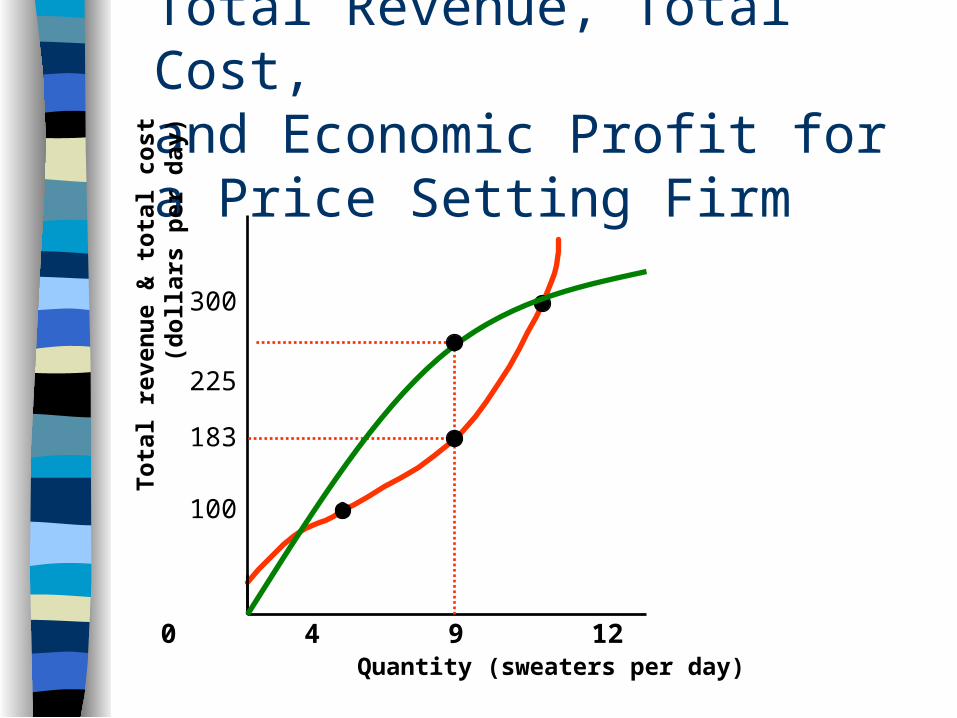
Price Taking FirmT
otal
rev
enu
e &
tot
al c
ost
(do
llar
s pe
r d
ay)
Quantity (sweaters per day)0 4 9 12
100
300
183
225
Economicloss
Economicprofit =TR - TC
TR
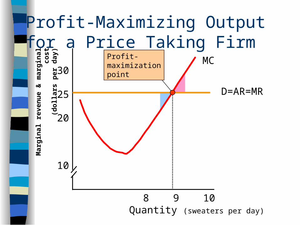
Profit-Maximizing Output for a Price Taking Firm
Quantity (sweaters per day)
8 9 10
10
20
30
Mar
gin
al r
even
ue
& m
argi
nal
cos
t (
dol
lars
per
day
)
25
Profit-maximizationpoint
D=AR=MR
MC
Total Revenue, Total Cost,and Economic Profit for a Price Setting Firm
Quantity (sweaters per day)
Tot
al r
even
ue
& t
otal
cos
t (
doll
ars
per
day
)
0 4 9 12
100
300
183
225
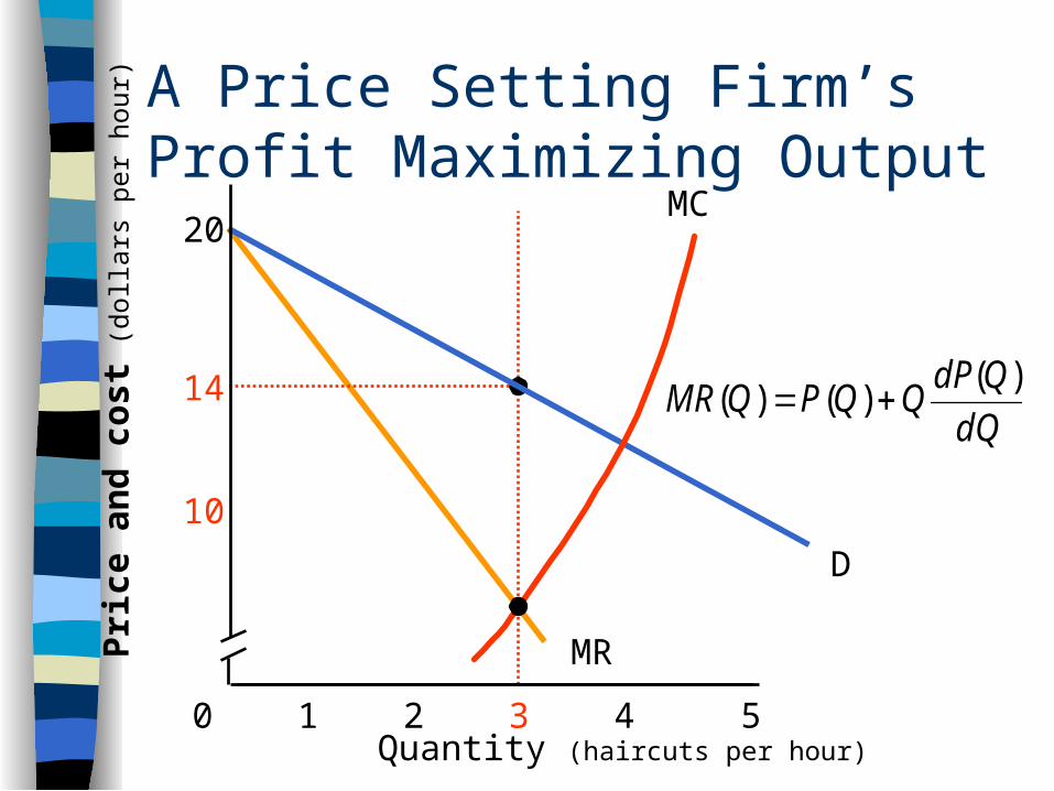
A Price Setting Firm’s Profit Maximizing Output
Pri
ce a
nd
cos
t (do
llar
s pe
r ho
ur)
0 1 2 3 4 5
10
14
20
Quantity (haircuts per hour)
D
MR
MC
dQ
QdPQQPQMR
)()()(
Price Taking Firm
Characteristics of Perfect Competition
– Many firms, each selling an identical product
– Many buyers
– No restrictions on entry into the industry
– Firms in the industry have no advantage over potential new
entrants
– Firms and buyers are well informed about prices of the
products of each firm in the industry
As a result of these characteristics, perfect competitors are
price takers.
Price takers -- firms that cannot influence the market price
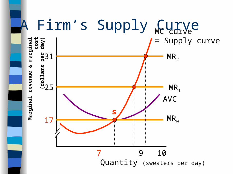
A Firm’s Supply CurveM
argi
nal
rev
enu
e &
mar
gin
al c
ost
(d
olla
rs p
er d
ay)
Quantity (sweaters per day)
7 9 10
17
25
31
MC curve = Supply curve
AVC
MR0
s
MR2
MR1
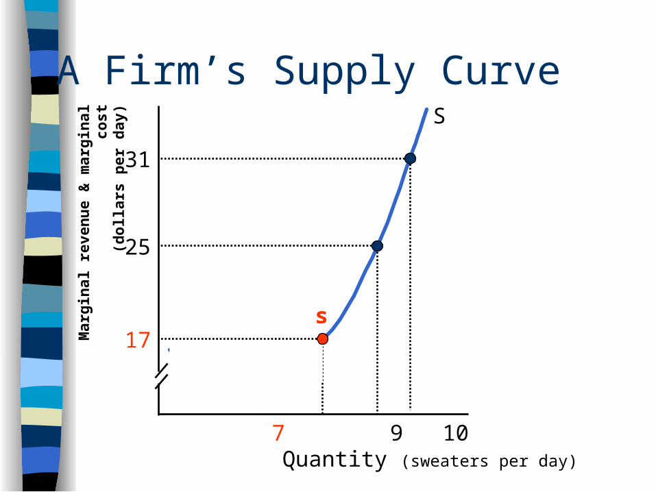
A Firm’s Supply Curve
Quantity (sweaters per day)
7 9 10
17
25
31
Mar
gin
al r
even
ue
& m
argi
nal
cos
t (
dol
lars
per
day
)S
s
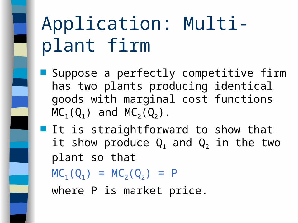
Application: Multi-plant firm
Suppose a perfectly competitive firm has two plants producing identical goods with marginal cost functions MC1(Q1) and MC2(Q2).
It is straightforward to show that it show produce Q1 and Q2 in the two plant so that
MC1(Q1) = MC2(Q2) = P
where P is market price.
Price Setting Firm
Price Setting Firm and How Monopoly Arises
The simplest form of price setting firm is monopoly
A monopoly is an industry that produces a good or service – for which no close substitute exists and – in which there is one supplier that is
protected from competition by a barrier preventing the entry of new firms.
Barriers to Entry
Key input owned by a firm– DeBeers, a South African firm that controls
more than 80 percent of the world’s supply of natural diamonds.
But most monopolies arise from two other types of barrier: legal barriers and natural barriers
Barriers to Entry
Legal Barriers to Entry– In a legal monopoly competition and entry is restricted by the
granting of a public franchise, government license, patent, or copyright.
– E.g. Microsoft is the only firm that is allowed to produce Window 98, etc. HK Town gas. China light
Natural Barriers to Entry– A natural monopoly results from a situation in which one firm can
supply the entire market at a lower price than two or more firms can.
– Example: Electric utility– A market used to be thought as a natural monopoly may turn out
to be no longer the case as technology progresses
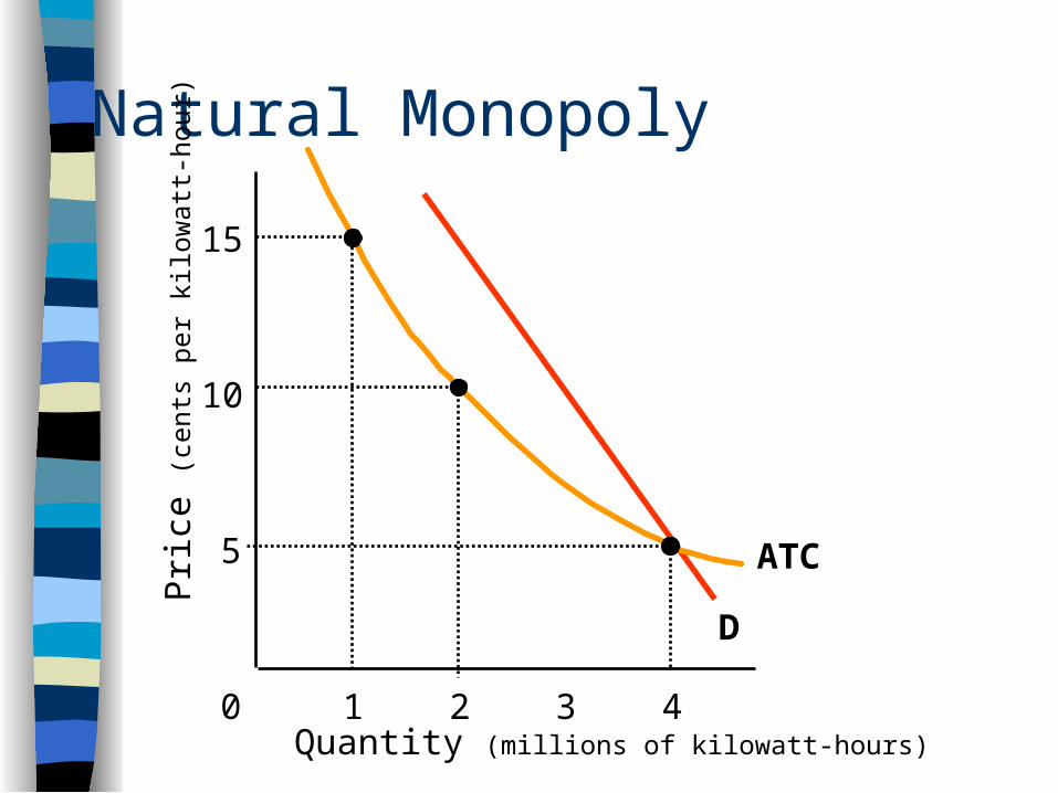
Natural Monopoly
Quantity (millions of kilowatt-hours)
5
10
15
0 1 2 3 4
D
Pri
ce (c
ents
per
kil
owat
t-ho
ur)
ATC
Monopoly Price-Setting Strategies Price discrimination is the practice of
selling different units of a good or service for different prices.
A single-price monopoly is a firm that must sell each unit of its output for the same price.
Single-Price Monopoly
The firm’s demand curve is the market demand curve.
Marginal revenue is not the same as the market price.
There is no supply curve for a monopoly.
Price and Output Decision
The competitive firm is a price taker, whereas the monopoly influences its price.
For the monopoly, price exceeds marginal revenue, thus price exceeds marginal cost.
Profit is maximized where MC = MR Monopolists can earn economic profits--firms
cannot enter due to barriers to entry.
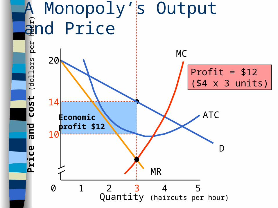
A Monopoly’s Output and PriceP
rice
an
d c
ost (
doll
ars
per
hour
)
0 1 2 3 4 5
10
14
20
Quantity (haircuts per hour)
ATCEconomicprofit $12
Profit = $12($4 x 3 units)
D
MR
MC
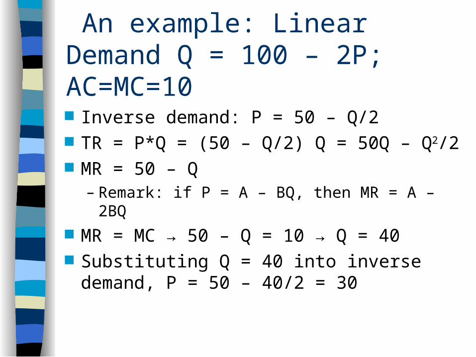
An example: Linear Demand Q = 100 – 2P; AC=MC=10
Inverse demand: P = 50 – Q/2 TR = P*Q = (50 – Q/2) Q = 50Q – Q2/2 MR = 50 – Q
– Remark: if P = A – BQ, then MR = A – 2BQ MR = MC → 50 – Q = 10 → Q = 40 Substituting Q = 40 into inverse
demand, P = 50 – 40/2 = 30
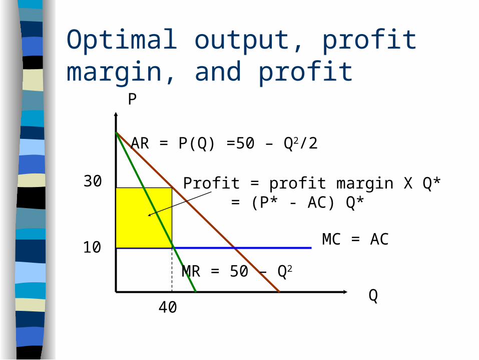
Optimal output, profit margin, and profit
MC = AC
AR = P(Q) =50 – Q2/2
Q
P
Profit = profit margin X Q*= (P* - AC) Q*
30
10
40
MR = 50 – Q2
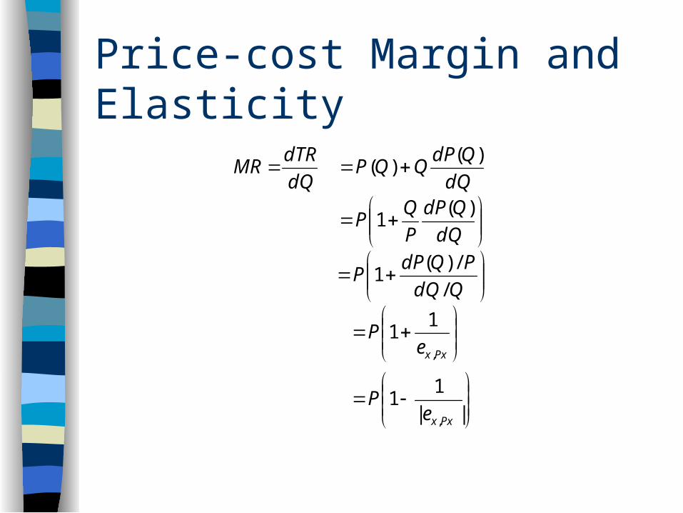
Price-cost Margin and Elasticity
||
11
11
/
/)(1
)(1
)()(
,
,
Pxx
Pxx
eP
eP
QdQ
PQdPP
dQ
QdP
P
QP
dQ
QdPQQP
dQ
dTRMR
Price-cost market and
||
1margincost -price
||
11
,
,
Pxx
Pxx
eP
MCPe
PMRMC
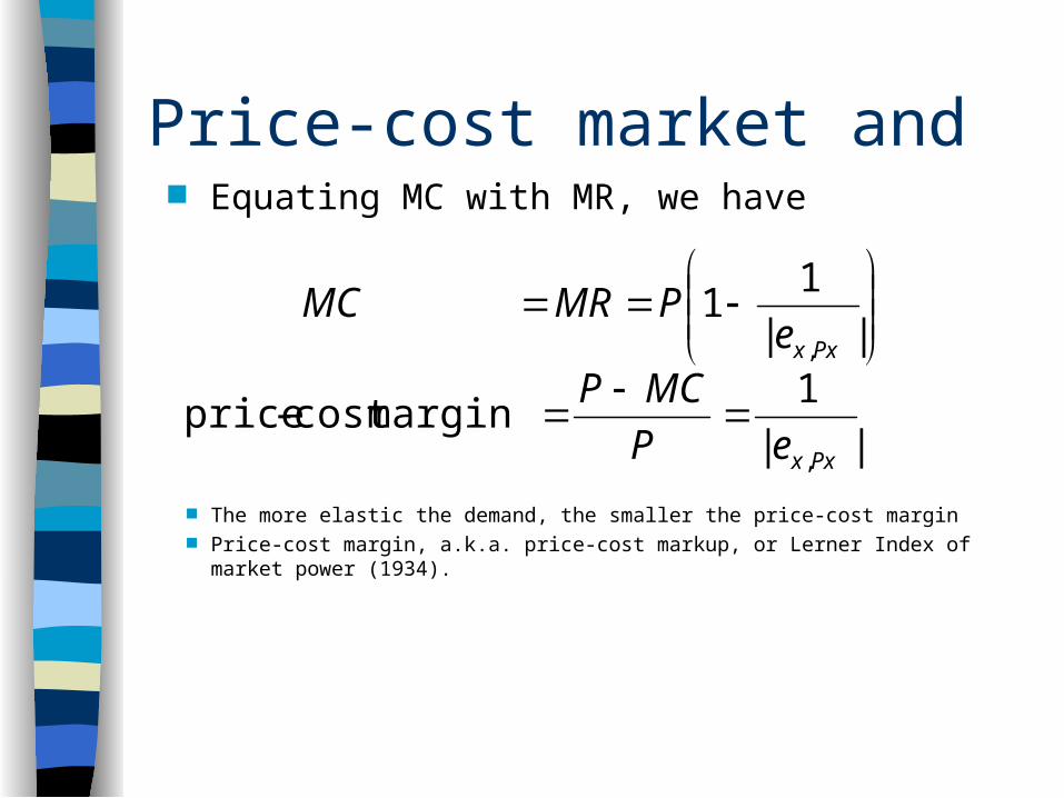
Equating MC with MR, we have
The more elastic the demand, the smaller the price-cost margin Price-cost margin, a.k.a. price-cost markup, or Lerner Index of market power (1934).
Competition and Efficiency
Efficiency is achieved when all the gains from trade have been realized (social welfare is maximized).
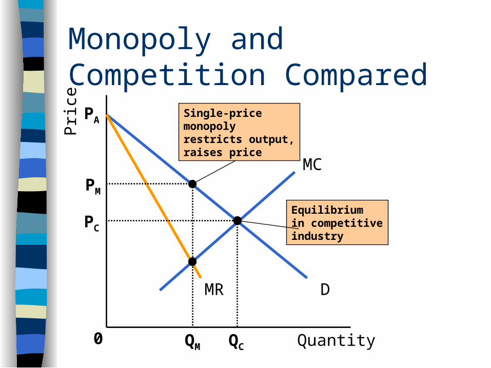
Monopoly andCompetition Compared
Pri
ce
Quantity
PA
PM
PC
0
DMR
MC
QM QC
Single-pricemonopolyrestricts output,raises price
Equilibriumin competitiveindustry
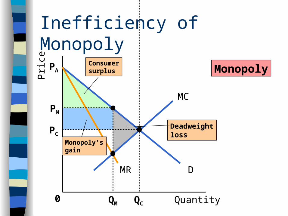
Inefficiency of MonopolyP
rice
Quantity
PA
PM
0
DMR
MC
QM QC
PC
Consumersurplus
Monopoly’sgain
Deadweightloss
Monopoly
Gains from Monopoly
Economies of Scale and Scope– Lowers average total cost and a greater
range of goods produced
Incentives to Innovate – The attempt to apply new knowledge in the
production process and obtain a patent
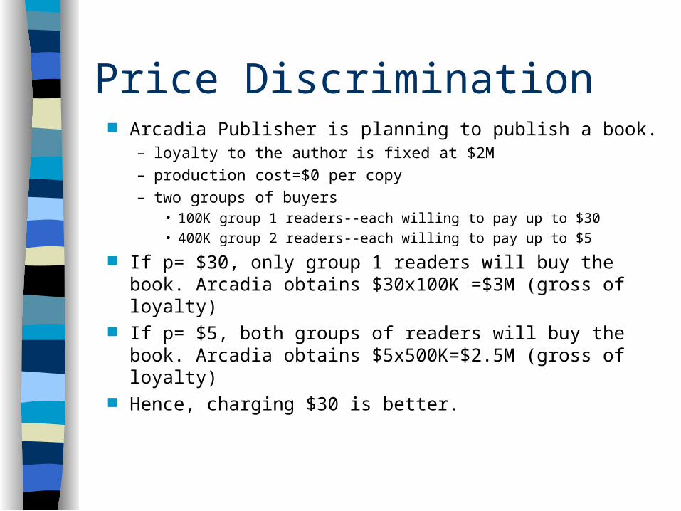
Price Discrimination Arcadia Publisher is planning to publish a book.
– loyalty to the author is fixed at $2M– production cost=$0 per copy– two groups of buyers
• 100K group 1 readers--each willing to pay up to $30• 400K group 2 readers--each willing to pay up to $5
If p= $30, only group 1 readers will buy the book. Arcadia obtains $30x100K =$3M (gross of loyalty)
If p= $5, both groups of readers will buy the book. Arcadia obtains $5x500K=$2.5M (gross of loyalty)
Hence, charging $30 is better.
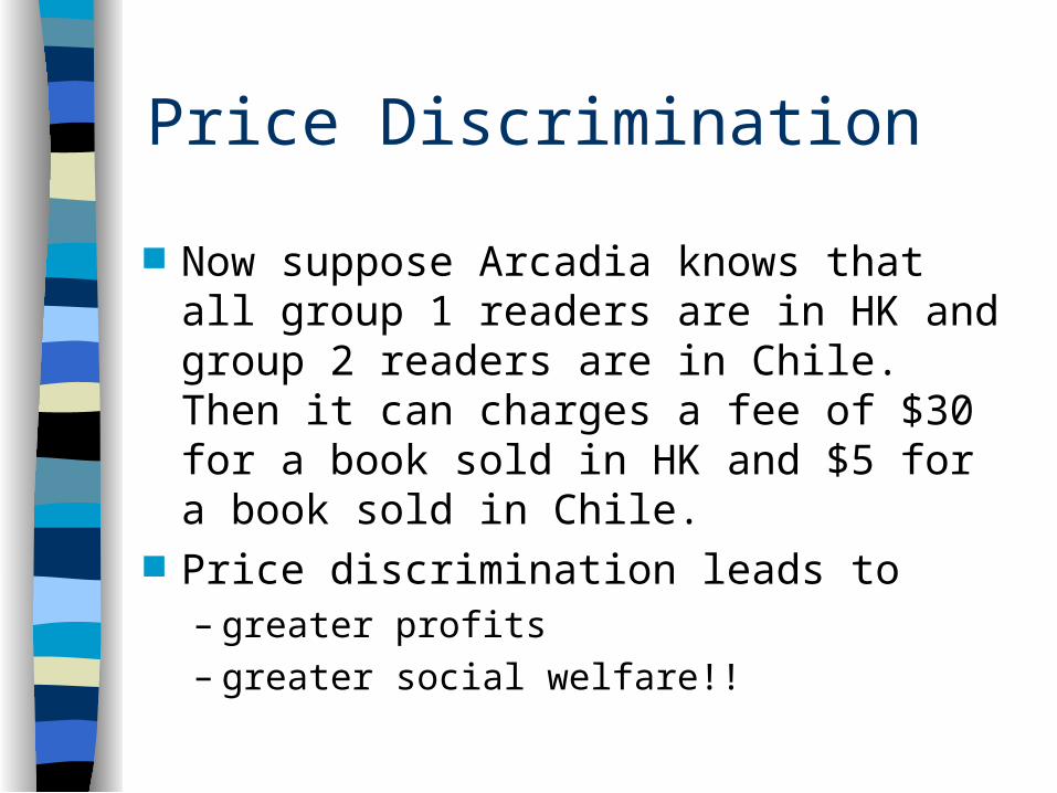
Price Discrimination
Now suppose Arcadia knows that all group 1 readers are in HK and group 2 readers are in Chile. Then it can charges a fee of $30 for a book sold in HK and $5 for a book sold in Chile.
Price discrimination leads to– greater profits– greater social welfare!!
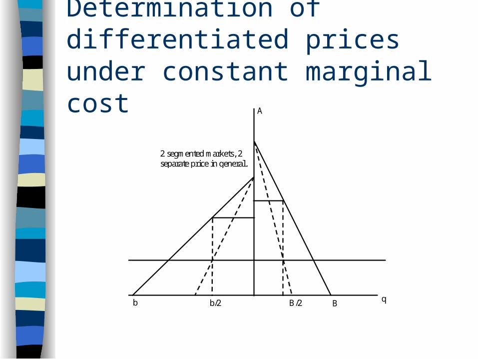
Determination of differentiated prices under constant marginal cost
A
q b b/2 B B/2
2 segmented markets, 2 separate price in general.
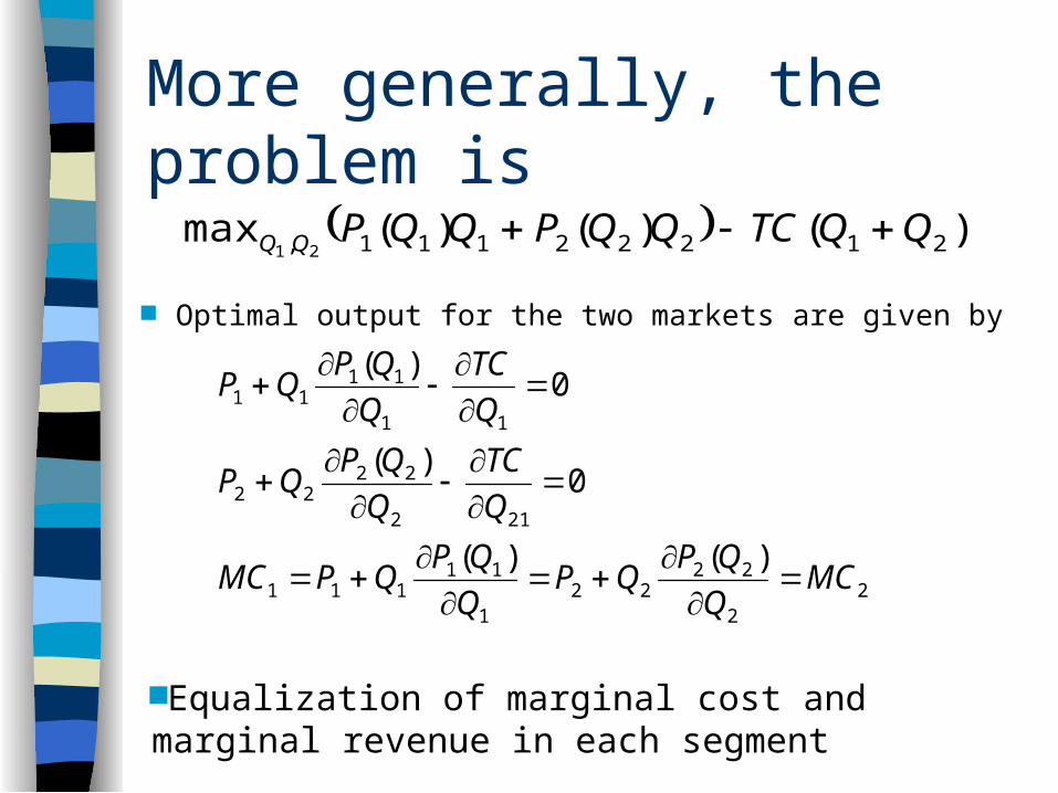
More generally, the problem is
)()()(max 21222111, 21QQTCQQPQQPQQ
Optimal output for the two markets are given by
22
2222
1
11111
212
2222
11
1111
)()(
0)(
0)(
MCQ
QPQP
Q
QPQPMC
Q
TC
Q
QPQP
Q
TC
Q
QPQP
Equalization of marginal cost and marginal revenue in each segment

Evidence of Geographic Price Discrimination
Parallel imports--unauthorized flows of genuine products across countries that compete with authorized distribution channels (ranging from deluxe cars to cheap beer)
It is often thought that parallel imports of HK made movie and music products back into HK market adversely affects the very survival of HK movie and music industry.
Price Discrimination: How to separate different customers
Coupons--those people who have lower time cost will collect and use coupons to get a discount; they are likely to have lower maximum willingness to pay as well (Sincere VIP card works similarly)
In 1999, CTI charged different fees for its registered IDD users--37cents/min to US for smart users who made a double registration; $2.9 /min for not-so-smart users who did not (c.w. HKTC’s 001 and 0060).
Educational edition--software companies charge a substantial lower price to teachers and students for their software

Price Discrimination: How to separate different customers
Hardcover vs paperback--readers of lower maximum willingness to pay are more patient; hence publishing a paperback later attract these buyers without affecting sale to hardcover buyers (compared w. seasonal sales in department stores)--production differentiation in general
Different prices for different geographic locations– golf clubs are much more expensive in HK than in
the US (HK$4.5K vs US$250)– tennis ball--HK’s price is two or three times that in
the US
Competitive Markets
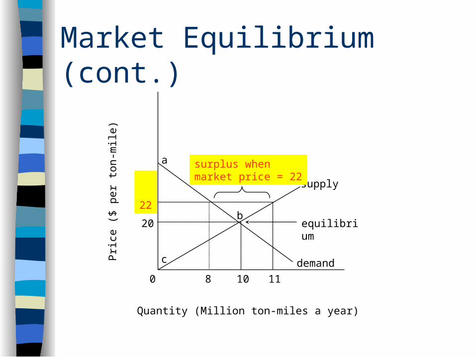
Market Equilibrium
Equilibrium is defined as the price at which the quantity demanded equals the quantity supplied (so markets clear)
– While all five conditions for perfect competition are (obviously) never fully satisfied, the model is still useful as frame of reference.
When a market is out of equilibrium, market forces push the price towards equilibrium
Excess supply (a.k.a., surplus) -- This triggers a price decrease
Excess demand (a.k.a., shortage) --This triggers a price increase
0
20
8 10 11
supply
demand
a
b
c
equilibrium
Quantity (Million ton-miles a year)
Pri
ce (
$ p
er
ton
-mil
e)
Market Equilibrium (cont.)
22
surplus when market price = 22
Invisible Hand
Social welfare (SW) = net gains from production and trade In the absence of tax, SW = buyer surplus + seller surplus In the presence of tax, SW = buyer surplus + seller surplus
+ tax revenue An outcome is efficient if the SW cannot be further
increased. [taxation cannot increase SW, to be shown shortly]
Perfect competition is efficient, in which– marginal benefit = price– marginal cost = price– single price in market
Price Ceiling
Upper limit that sellers can lawfully charge and buyers can lawfully pay rent control regulated price for electricity
Price Floor
Lower limit that sellers can charge and buyers can pay minimum wage agricultural price supports
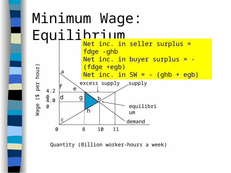
Minimum Wage: Equilibrium
0
4.20
8 10 11
supply
demand
a
b
c
equilibrium
excess supply
Quantity (Billion worker-hours a week)
Wage (
$ p
er
hour)
4.00
Net inc. in seller surplus = fdge -ghbNet inc. in buyer surplus = - (fdge +egb)Net inc. in SW = - (ghb + egb)
ef
d g
h
Minimum Wage: Losses
deadweight losses -- sellers willing to provide item at price that buyers willing to pay, but provision doesn’t occur
price elasticities of demand and supply
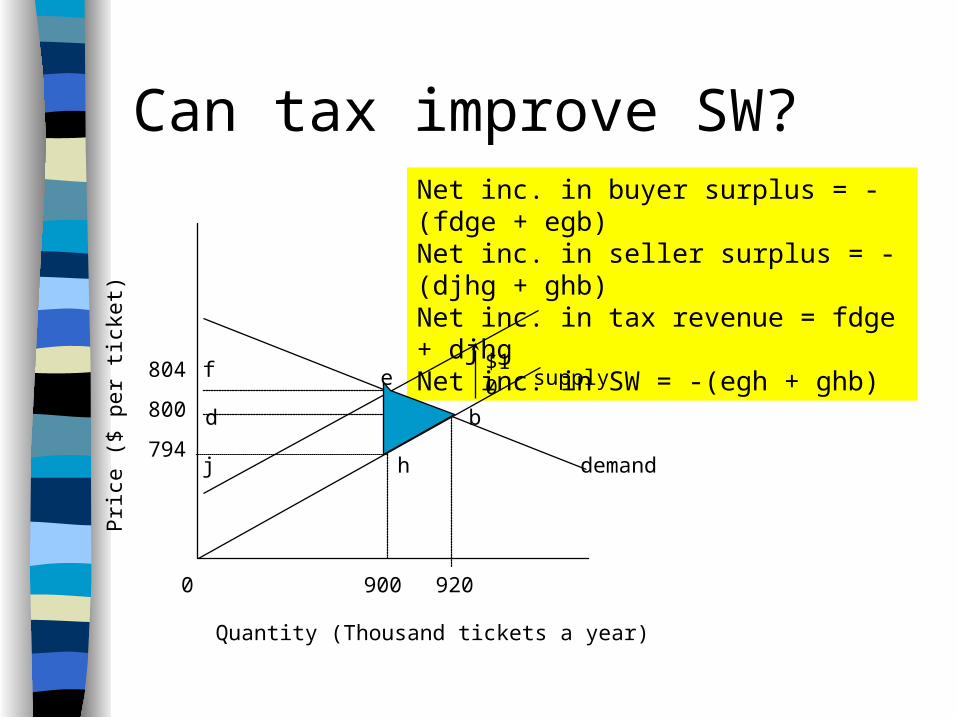
Can tax improve SW?Net inc. in buyer surplus = -(fdge + egb) Net inc. in seller surplus = -(djhg + ghb) Net inc. in tax revenue = fdge + djhgNet inc. in SW = -(egh + ghb)
0
800
900
e
Quantity (Thousand tickets a year)
Pri
ce (
$ p
er
tick
et)
supply
demand
$10
b
h
804
794
920
f
d
j
g
Tax: Does it matter whom the tax is imposed upon: sellers or buyers? If an excise tax of $10 is levied on sellers, the
sellers will be willing to supply the same quantity as before only when the price is increased by $10. [upper shifting of supply, demand unmoved]
If an excise tax of $10 is levied directly on buyers, the buyers will buy the same quantity as before only when the price charged by sellers is reduced by $10. [downward shifting of demand, supply unmoved.]
The outcomes under the two scenarios are the same


