
NBP Working Paper No. 257
Early warning models of banking crises applicable to non-crisis countries
Piotr Bańbuła, Marcin Pietrzak

Economic InstituteWarsaw, 2017
NBP Working Paper No. 257
Early warning models of banking crises applicable to non-crisis countries
Piotr Bańbuła, Marcin Pietrzak

Published by: Narodowy Bank Polski Education & Publishing Department ul. Świętokrzyska 11/21 00-919 Warszawa, Poland phone +48 22 185 23 35 www.nbp.pl
ISSN 2084-624X
© Copyright Narodowy Bank Polski, 2017
Piotr Bańbuła – Narodowy Bank Polski and Warsaw School of Economics. Corresponding author; [email protected]
Marcin Pietrzak – Narodowy Bank Polski
We would like to thank Martin O’Brien, Mateusz Pipień, Dobromił Serwa and Piotr Wdowiński, as well as participants of the NBP seminar, 36th International Symposium on Forecasting in Santander and 2nd Policy Research Conference of the ECBN in Ljubljana for comments and suggestions on earlier version of the paper. All remaining errors are our own. Any views expressed are those of the authors and do not necessarily reflect the views of Narodowy Bank Polski or other institutions they are affiliated with.

ContentsAbstract 4
1 Introduction 5
2 Literature review 8
3 Data and method 11
3.1 Data 113.2 Method 14
3.2.1 Financial cycle 143.2.2 Non-parametric methods and binary choice models 173.2.3 Evaluation of signals 20
4 Empirical results 23
4.1 Models with one explanatory variable 234.2 Stability of signals accuracy 254.3 Models with credit gap and three explanatory variables 28
5 Conclusions 32
References 33
Appendix A Data description and sources 37
Appendix B Logistic regression models 38
Appendix C ROC curves 39
3NBP Working Paper No. 257

2
Abstract
We built Early Warning Models (EWM) for determining the optimal moment
for build-up phase of the countercyclical capital buffer. For this purpose we
estimate a number of early warning models based on the wide panel of
countries. We test many potential variables from the early 1970s until 2014,
their combinations, and the stability of their signals. Our setting includes
country-specific information without using country-specific effects. This
allows for direct application of EWM we obtain to any country, including
those that have not experienced a banking crisis. Models with three
explanatory variables outperform models with smaller number of variates.
The probability of extracting a correct signal from best-performing EWM
exceeds 0.9. We find that low levels of VIX tend to precede crises, and this was
also true before 2006. This corroborates Minsky’s hypothesis about periodic
underestimation of risk in the financial sector. Other variables that generate
signals with the highest accuracy and stability are those associated with credit
growth, property prices and growth in the contribution of financial sector to
GDP. This last finding suggests that substantial increases in measured value
added of the financial sector seem to reflect augmented exposure to systemic
risk, rather than welfare improvements.
JEL codes: E44, G01, G21
Keywords: countercyclical capital buffer, early warning models, financial
stability.
Narodowy Bank Polski4
Abstract

3
1. Introduction
Outbreak of the most severe financial crisis in the last decades has increased
interest in the tools that would be able to reduce systemic risk. One of them is
countercyclical capital buffer, which is designed by the Basel Committee on
Banking Supervision (Basel III) and is implemented, among others, within the
framework of the Directive of the European Parliament and of the Council
2013/36/ EU of 26 June 2013. (CRD IV). Even though CRD IV obliges the
authority responsible for macroprudential supervision to calculate a
benchmark for the buffer rate, it allows the final decision to differ from the
reference level (this is called guided discretion). Three crucial issues related
to the use of countercyclical capital buffer are: (i) when to build up the buffer,
(ii) what is the optimal buffer rate level, (iii) when the buffer should be
released.
This study focuses on the fundamental, first issue. According to the
recommendation of the ESRB (2014) countercyclical capital buffer benchmark
rate is calculated as a linear function of only one variable (credit gap) that is
obtained under relatively strong assumptions (i.e. the financial cycle is
assumed to last over 20 years in all countries). However, rules suggested by
the ESRB do not preclude use of other quantitative or qualitative methods
since having broader information set should allow for better decisions. In this
respect we answer two basic questions: (i) which variables offer best warning
signals before the crisis?; (ii) how much does one gain by simultaneously
including information from more than one variable?
We analyse early warning properties of many macroeconomic and financial
indicators in nearly fifty countries starting (where possible) in the 1970s until
2
Abstract
We built Early Warning Models (EWM) for determining the optimal moment
for build-up phase of the countercyclical capital buffer. For this purpose we
estimate a number of early warning models based on the wide panel of
countries. We test many potential variables from the early 1970s until 2014,
their combinations, and the stability of their signals. Our setting includes
country-specific information without using country-specific effects. This
allows for direct application of EWM we obtain to any country, including
those that have not experienced a banking crisis. Models with three
explanatory variables outperform models with smaller number of variates.
The probability of extracting a correct signal from best-performing EWM
exceeds 0.9. We find that low levels of VIX tend to precede crises, and this was
also true before 2006. This corroborates Minsky’s hypothesis about periodic
underestimation of risk in the financial sector. Other variables that generate
signals with the highest accuracy and stability are those associated with credit
growth, property prices and growth in the contribution of financial sector to
GDP. This last finding suggests that substantial increases in measured value
added of the financial sector seem to reflect augmented exposure to systemic
risk, rather than welfare improvements.
JEL codes: E44, G01, G21
Keywords: countercyclical capital buffer, early warning models, financial
stability.
5NBP Working Paper No. 257
Chapter 1

4
2014. Among the novel variables we include VIX and contribution of the
financial sector to GDP and two hypotheses associated with these variables.
The VIX, often called a fear index, reflects joint effect of risk perception and
attitude toward risk by investors. If financial sector has tendency to be overly
optimistic and take excessive risk, which are followed by crises, as suggested
by Minsky, low levels of VIX should precede crises. It has also been argued
that measurement of contribution of financial sector is flawed (Haldane et al.
2010), and largely reflects risk taken by the sector rather than value added. If
that is indeed the case, unusually high share of financial sector in GDP growth
is expected to reflect unusually high levels of risk exposure that are bound to
sometimes materialise as crisis. We test both these hypotheses.
We evaluate the performance of all indicators using their levels, dynamics and
deviations from trend in period ranging from 5 to 16 quarters before the actual
crisis. Cyclical components are extracted by adjusting smoothing parameter
of the HP filter such that it corresponds to the financial cycle in a given
country, instead of assuming that the financial cycle has the same length in all
countries. We do not use fixed effects, but include country-specific
characteristic by using variables that are standardised using data for each
country. Fixed effects improve model performance, but essentially prevent
model use in countries that have not experienced crisis (fixed effect would
automatically push crisis probability to zero and would likely dominate all
explanatory variables also in future). We evaluate individual variables by not
only checking accuracy of their signals, but also its stability, i.e. we assess
accuracy in sample excluding current crisis, and check for out-of-sample
performance during the recent crisis. The best indicators are then included in
early warning models of banking crises as explanatory variables. We
Narodowy Bank Polski6

5
subsequently evaluate their statistical properties of models with one, two,
three and more explanatory variables. On the basis of the relative costs of
missing the crisis and false alarm of a crisis we calculate thresholds of
probability which signals crisis risk. We end up with signals that correctly
discriminate between tranquil and crisis states in more than 90% of cases, with
true positive rate in excess of 0.75 and false positive rate below 0.1.
Study is divided into four parts. Part 2 discusses the results of studies
conducted so far. Part 3 contains a description of the data and method, while
Part 4 discusses empirical results. Paper concludes with a summary.
4
2014. Among the novel variables we include VIX and contribution of the
financial sector to GDP and two hypotheses associated with these variables.
The VIX, often called a fear index, reflects joint effect of risk perception and
attitude toward risk by investors. If financial sector has tendency to be overly
optimistic and take excessive risk, which are followed by crises, as suggested
by Minsky, low levels of VIX should precede crises. It has also been argued
that measurement of contribution of financial sector is flawed (Haldane et al.
2010), and largely reflects risk taken by the sector rather than value added. If
that is indeed the case, unusually high share of financial sector in GDP growth
is expected to reflect unusually high levels of risk exposure that are bound to
sometimes materialise as crisis. We test both these hypotheses.
We evaluate the performance of all indicators using their levels, dynamics and
deviations from trend in period ranging from 5 to 16 quarters before the actual
crisis. Cyclical components are extracted by adjusting smoothing parameter
of the HP filter such that it corresponds to the financial cycle in a given
country, instead of assuming that the financial cycle has the same length in all
countries. We do not use fixed effects, but include country-specific
characteristic by using variables that are standardised using data for each
country. Fixed effects improve model performance, but essentially prevent
model use in countries that have not experienced crisis (fixed effect would
automatically push crisis probability to zero and would likely dominate all
explanatory variables also in future). We evaluate individual variables by not
only checking accuracy of their signals, but also its stability, i.e. we assess
accuracy in sample excluding current crisis, and check for out-of-sample
performance during the recent crisis. The best indicators are then included in
early warning models of banking crises as explanatory variables. We
7NBP Working Paper No. 257
Introduction

6
2. Literature review
Outbreak of the recent financial crisis intensified research focusing on the
usefulness of macroeconomic and financial variables as indicators of early
warning of imminent banking and more generally financial crises. One of the
first such studies by Borio and Drehmann (2009) uses the signal extraction
method (Kaminsky and Reinhart, 1999) and suggests that in the case of the US
early warning indicators would have signal significant imbalances in the
financial sector already in 2004. According to the study variables connected
with credit, real estate prices and equity prices have the highest predictive
ability. In addition, authors suggest that the analysis comprising several
variables gives better results than in case of one variable. In the following
years, a further increase of interest related to this field was observed. As a
result, there has been a substantial growth in the number of research papers
related to Early Warning Models. For instance Drehmann et al. (2010) used
the same methodology as Borio and Drehmann (2009) did. They analysed 7
variables for 36 developed countries. Credit gap, i.e. the deviation of ratio of
credit to GDP from the long-term trend, correctly indicates 72% of crises in
the sample (overall there are 25 crises) with the ratio of false signals to
accurate signals (noise-to-signal ratio - NtS) reaching 20%. Real estate prices
are equally useful. This variable correctly indicates crises in 67% of cases
which is achieved with NtS of 22%. The value added of their study is the
attempt to identify the length of financial cycle. When estimating the cyclical
component of analysed variables the authors took into account several
different smoothing parameters λ of Hodrick-Prescott filter (1997). They
assume that credit cycles are of the same length as the business cycles and that
they are respectively: two, three and four times longer. According to the
8
discriminate between tranquil and crisis periods. It should be noted, however,
that such a high score would not have been achieved had it not taken into
account country-specific effects, which increase accuracy1. Similarly to the
studies discussed previously Lainà et al. (2015) estimate a series of logistic
regression models for panel data of 11 EU Member States. Authors argue that
narrowing the number of countries in the sample (although the reverse trend
in the literature is observed) is needed to achieve larger homogeneity of
analysed countries. The results support the use of loans to deposits ratio and
property prices as those variables that warn about banking crises in the most
accurate way. Additionally, the authors analyse the cumulative probability of
banking crisis outbreak in the horizon of several quarters that is obtained by
multiplying the individual probabilities from a logistic regression model,
which implicitly hinges on the assumption that individual probabilities of
crisis are independent. Such assumption does not reflect the characteristics of
phenomena in question, which in turn means that the resulting cumulative
probabilities may differ from the actual ones. Another interesting work is the
one by Juks and Melander (2012) that points out that before making a decision
about the countercyclical capital buffer one should disaggregate the data by
sector (this is possible for the credit gap). Using data for Sweden, authors
show that excessive credit growth in the late 80s was driven by the growth in
lending to the non-financial corporations, while the credit boom in the years
preceding the recent financial crisis was due to the rise in households’ debt.
Finally, it is worth taking a look at two studies which check the benefits of
extending the sample such that is starts in: the beginning of the last century
in Finland (Laine et al., 2015) and in 1861 in Italy (Alessandri et al., 2015). The
1 Catão and Milesi-Ferretti (2014) suggest that the increase of AUROC resulting from country-specific effects
totals approximately 20 percentage points. In our sample it artificially "improves" the quality of predictive signals (AUROCs are higher by 20-30 percentage points depending on the variable).
Narodowy Bank Polski8
Chapter 2

7
principle proposed by Ravn and Uhlig (2002) values of smoothing parameters
λ are equal to: 1,600; 25,000; 125,000 and 400,000. The most accurate signals
were generated by the credit gap under the assumption that credit cycles are
four times longer than business cycles. Longer duration of financial cycles
relative to the business cycle was confirmed in later studies dedicated to the
issue of financial cycle length (see Drehmann et al., 2012; Schüler et al., 2015).
Importance of proper and early signals of imminent banking crisis was
highlighted in the study by Babecký et al. (2013) which uses a panel vector
autoregression models. Authors confirmed a hypothesis that the currency and
debt crises are preceded by banking crises. In the same study, based on the
data from 40 developed countries using Bayesian averaging, authors identify
variables that should be monitored in order to avoid banking crises. These
include credit, the inflow of foreign direct investment and money market
interest rates. Drehmann and Juselius (2012) postulate the inclusion of
variable called debt service ratio (DSR), which is an aggregate measure of a
debt service costs relative to aggregate income. The analysis carried out by
Drehmann and Juselius (2014) confirms the usefulness of this indicator, which
at shorter horizons, i.e. two years before a crisis, generates more accurate
signals than the credit gap. The conclusions regarding the usefulness of credit
gap are also confirmed in a study by Behn et al. (2013). That analysis covers
23 EU Member States and uses logistic regression models with fixed effects
(country-specific fixed effects). The main caveat of this approach is that due
to the inclusion of the country-specific effects, those models have limited
usefulness when it comes to the issuing early warning of crises in countries
which have never experienced such phenomena. Accuracy of signals
generated with those models is high since in over 90% of cases they correctly
6
2. Literature review
Outbreak of the recent financial crisis intensified research focusing on the
usefulness of macroeconomic and financial variables as indicators of early
warning of imminent banking and more generally financial crises. One of the
first such studies by Borio and Drehmann (2009) uses the signal extraction
method (Kaminsky and Reinhart, 1999) and suggests that in the case of the US
early warning indicators would have signal significant imbalances in the
financial sector already in 2004. According to the study variables connected
with credit, real estate prices and equity prices have the highest predictive
ability. In addition, authors suggest that the analysis comprising several
variables gives better results than in case of one variable. In the following
years, a further increase of interest related to this field was observed. As a
result, there has been a substantial growth in the number of research papers
related to Early Warning Models. For instance Drehmann et al. (2010) used
the same methodology as Borio and Drehmann (2009) did. They analysed 7
variables for 36 developed countries. Credit gap, i.e. the deviation of ratio of
credit to GDP from the long-term trend, correctly indicates 72% of crises in
the sample (overall there are 25 crises) with the ratio of false signals to
accurate signals (noise-to-signal ratio - NtS) reaching 20%. Real estate prices
are equally useful. This variable correctly indicates crises in 67% of cases
which is achieved with NtS of 22%. The value added of their study is the
attempt to identify the length of financial cycle. When estimating the cyclical
component of analysed variables the authors took into account several
different smoothing parameters λ of Hodrick-Prescott filter (1997). They
assume that credit cycles are of the same length as the business cycles and that
they are respectively: two, three and four times longer. According to the
8
discriminate between tranquil and crisis periods. It should be noted, however,
that such a high score would not have been achieved had it not taken into
account country-specific effects, which increase accuracy1. Similarly to the
studies discussed previously Lainà et al. (2015) estimate a series of logistic
regression models for panel data of 11 EU Member States. Authors argue that
narrowing the number of countries in the sample (although the reverse trend
in the literature is observed) is needed to achieve larger homogeneity of
analysed countries. The results support the use of loans to deposits ratio and
property prices as those variables that warn about banking crises in the most
accurate way. Additionally, the authors analyse the cumulative probability of
banking crisis outbreak in the horizon of several quarters that is obtained by
multiplying the individual probabilities from a logistic regression model,
which implicitly hinges on the assumption that individual probabilities of
crisis are independent. Such assumption does not reflect the characteristics of
phenomena in question, which in turn means that the resulting cumulative
probabilities may differ from the actual ones. Another interesting work is the
one by Juks and Melander (2012) that points out that before making a decision
about the countercyclical capital buffer one should disaggregate the data by
sector (this is possible for the credit gap). Using data for Sweden, authors
show that excessive credit growth in the late 80s was driven by the growth in
lending to the non-financial corporations, while the credit boom in the years
preceding the recent financial crisis was due to the rise in households’ debt.
Finally, it is worth taking a look at two studies which check the benefits of
extending the sample such that is starts in: the beginning of the last century
in Finland (Laine et al., 2015) and in 1861 in Italy (Alessandri et al., 2015). The
1 Catão and Milesi-Ferretti (2014) suggest that the increase of AUROC resulting from country-specific effects
totals approximately 20 percentage points. In our sample it artificially "improves" the quality of predictive signals (AUROCs are higher by 20-30 percentage points depending on the variable).
9NBP Working Paper No. 257
Literature review

9
second one calls into question the benefits of extending sample to get more
precise estimates of the credit gap.
8
discriminate between tranquil and crisis periods. It should be noted, however,
that such a high score would not have been achieved had it not taken into
account country-specific effects, which increase accuracy1. Similarly to the
studies discussed previously Lainà et al. (2015) estimate a series of logistic
regression models for panel data of 11 EU Member States. Authors argue that
narrowing the number of countries in the sample (although the reverse trend
in the literature is observed) is needed to achieve larger homogeneity of
analysed countries. The results support the use of loans to deposits ratio and
property prices as those variables that warn about banking crises in the most
accurate way. Additionally, the authors analyse the cumulative probability of
banking crisis outbreak in the horizon of several quarters that is obtained by
multiplying the individual probabilities from a logistic regression model,
which implicitly hinges on the assumption that individual probabilities of
crisis are independent. Such assumption does not reflect the characteristics of
phenomena in question, which in turn means that the resulting cumulative
probabilities may differ from the actual ones. Another interesting work is the
one by Juks and Melander (2012) that points out that before making a decision
about the countercyclical capital buffer one should disaggregate the data by
sector (this is possible for the credit gap). Using data for Sweden, authors
show that excessive credit growth in the late 80s was driven by the growth in
lending to the non-financial corporations, while the credit boom in the years
preceding the recent financial crisis was due to the rise in households’ debt.
Finally, it is worth taking a look at two studies which check the benefits of
extending the sample such that is starts in: the beginning of the last century
in Finland (Laine et al., 2015) and in 1861 in Italy (Alessandri et al., 2015). The
1 Catão and Milesi-Ferretti (2014) suggest that the increase of AUROC resulting from country-specific effects
totals approximately 20 percentage points. In our sample it artificially "improves" the quality of predictive signals (AUROCs are higher by 20-30 percentage points depending on the variable).
10
3. Data and method
3.1 Data
Potential leading indicators were analysed based on the data from 47
countries - all EU member states and countries outside the EU, for which the
Bank for International Settlements (BIS) publishes data on credit extended to
private non-financial sector. Thus it is the largest panel of countries taken into
account compared with the studies in the literature. The availability of the
data about the credit was the only criterion to include given country to the
sample because many studies indicate that the variables connected with the
credit cycles (i.e. credit gap and DSR) are the most useful. Our analysis covers
the period from the first quarter of 1970 to the second quarter of 2014.
However quite often for the initial 10-20 years in the sample the data is not
available and it is especially common for the countries of Central and Eastern
Europe. Variables were analysed in levels, growth rates (quarterly, annual,
two-, three- and four-year) and cyclical deviations from respective long-term
trend. In summary, we take into account twelve variables, their ratios and
transformations, which results in more than fifty analysed indicators.
Description of the data and their sources can be found in Appendix A.
In addition to the variables analysed so far, we included proxies of situation
in financial or when possible banking sector. These are contribution of
financial sector to GDP growth2 (VA hereafter), banking sector index on
equity market and VIX. Inclusion of VIX proxies market price of global risk.
2 Statistical offices do not publish data on banking sector contribution to GDP, however in majority of countries
banking sector plays dominant role in financial system. Thus, financial sector contribution can be still useful in predicting banking crises.
Narodowy Bank Polski10

9
second one calls into question the benefits of extending sample to get more
precise estimates of the credit gap.
8
discriminate between tranquil and crisis periods. It should be noted, however,
that such a high score would not have been achieved had it not taken into
account country-specific effects, which increase accuracy1. Similarly to the
studies discussed previously Lainà et al. (2015) estimate a series of logistic
regression models for panel data of 11 EU Member States. Authors argue that
narrowing the number of countries in the sample (although the reverse trend
in the literature is observed) is needed to achieve larger homogeneity of
analysed countries. The results support the use of loans to deposits ratio and
property prices as those variables that warn about banking crises in the most
accurate way. Additionally, the authors analyse the cumulative probability of
banking crisis outbreak in the horizon of several quarters that is obtained by
multiplying the individual probabilities from a logistic regression model,
which implicitly hinges on the assumption that individual probabilities of
crisis are independent. Such assumption does not reflect the characteristics of
phenomena in question, which in turn means that the resulting cumulative
probabilities may differ from the actual ones. Another interesting work is the
one by Juks and Melander (2012) that points out that before making a decision
about the countercyclical capital buffer one should disaggregate the data by
sector (this is possible for the credit gap). Using data for Sweden, authors
show that excessive credit growth in the late 80s was driven by the growth in
lending to the non-financial corporations, while the credit boom in the years
preceding the recent financial crisis was due to the rise in households’ debt.
Finally, it is worth taking a look at two studies which check the benefits of
extending the sample such that is starts in: the beginning of the last century
in Finland (Laine et al., 2015) and in 1861 in Italy (Alessandri et al., 2015). The
1 Catão and Milesi-Ferretti (2014) suggest that the increase of AUROC resulting from country-specific effects
totals approximately 20 percentage points. In our sample it artificially "improves" the quality of predictive signals (AUROCs are higher by 20-30 percentage points depending on the variable).
8
discriminate between tranquil and crisis periods. It should be noted, however,
that such a high score would not have been achieved had it not taken into
account country-specific effects, which increase accuracy1. Similarly to the
studies discussed previously Lainà et al. (2015) estimate a series of logistic
regression models for panel data of 11 EU Member States. Authors argue that
narrowing the number of countries in the sample (although the reverse trend
in the literature is observed) is needed to achieve larger homogeneity of
analysed countries. The results support the use of loans to deposits ratio and
property prices as those variables that warn about banking crises in the most
accurate way. Additionally, the authors analyse the cumulative probability of
banking crisis outbreak in the horizon of several quarters that is obtained by
multiplying the individual probabilities from a logistic regression model,
which implicitly hinges on the assumption that individual probabilities of
crisis are independent. Such assumption does not reflect the characteristics of
phenomena in question, which in turn means that the resulting cumulative
probabilities may differ from the actual ones. Another interesting work is the
one by Juks and Melander (2012) that points out that before making a decision
about the countercyclical capital buffer one should disaggregate the data by
sector (this is possible for the credit gap). Using data for Sweden, authors
show that excessive credit growth in the late 80s was driven by the growth in
lending to the non-financial corporations, while the credit boom in the years
preceding the recent financial crisis was due to the rise in households’ debt.
Finally, it is worth taking a look at two studies which check the benefits of
extending the sample such that is starts in: the beginning of the last century
in Finland (Laine et al., 2015) and in 1861 in Italy (Alessandri et al., 2015). The
1 Catão and Milesi-Ferretti (2014) suggest that the increase of AUROC resulting from country-specific effects
totals approximately 20 percentage points. In our sample it artificially "improves" the quality of predictive signals (AUROCs are higher by 20-30 percentage points depending on the variable).
10
3. Data and method
3.1 Data
Potential leading indicators were analysed based on the data from 47
countries - all EU member states and countries outside the EU, for which the
Bank for International Settlements (BIS) publishes data on credit extended to
private non-financial sector. Thus it is the largest panel of countries taken into
account compared with the studies in the literature. The availability of the
data about the credit was the only criterion to include given country to the
sample because many studies indicate that the variables connected with the
credit cycles (i.e. credit gap and DSR) are the most useful. Our analysis covers
the period from the first quarter of 1970 to the second quarter of 2014.
However quite often for the initial 10-20 years in the sample the data is not
available and it is especially common for the countries of Central and Eastern
Europe. Variables were analysed in levels, growth rates (quarterly, annual,
two-, three- and four-year) and cyclical deviations from respective long-term
trend. In summary, we take into account twelve variables, their ratios and
transformations, which results in more than fifty analysed indicators.
Description of the data and their sources can be found in Appendix A.
In addition to the variables analysed so far, we included proxies of situation
in financial or when possible banking sector. These are contribution of
financial sector to GDP growth2 (VA hereafter), banking sector index on
equity market and VIX. Inclusion of VIX proxies market price of global risk.
2 Statistical offices do not publish data on banking sector contribution to GDP, however in majority of countries
banking sector plays dominant role in financial system. Thus, financial sector contribution can be still useful in predicting banking crises.
10
3. Data and method
3.1 Data
Potential leading indicators were analysed based on the data from 47
countries - all EU member states and countries outside the EU, for which the
Bank for International Settlements (BIS) publishes data on credit extended to
private non-financial sector. Thus it is the largest panel of countries taken into
account compared with the studies in the literature. The availability of the
data about the credit was the only criterion to include given country to the
sample because many studies indicate that the variables connected with the
credit cycles (i.e. credit gap and DSR) are the most useful. Our analysis covers
the period from the first quarter of 1970 to the second quarter of 2014.
However quite often for the initial 10-20 years in the sample the data is not
available and it is especially common for the countries of Central and Eastern
Europe. Variables were analysed in levels, growth rates (quarterly, annual,
two-, three- and four-year) and cyclical deviations from respective long-term
trend. In summary, we take into account twelve variables, their ratios and
transformations, which results in more than fifty analysed indicators.
Description of the data and their sources can be found in Appendix A.
In addition to the variables analysed so far, we included proxies of situation
in financial or when possible banking sector. These are contribution of
financial sector to GDP growth2 (VA hereafter), banking sector index on
equity market and VIX. Inclusion of VIX proxies market price of global risk.
2 Statistical offices do not publish data on banking sector contribution to GDP, however in majority of countries
banking sector plays dominant role in financial system. Thus, financial sector contribution can be still useful in predicting banking crises.
11NBP Working Paper No. 257
Chapter 3

11
Analysis of this variable has a purpose of checking whether global factors
influence probability of banking crisis. Adding VA hinges on the assumption
that the value added of this sector is to some extent a measure of risk-taking.
According to national accounts VA is calculated as:
Revenues-Costs-Amortization = Renumeration + Interests + Dividends + Taxes + Retained Earnings.
Equation above shows that high VA (so in particular of banking sector) might
not be connected with its contribution to the welfare, but rather with risk-
taking, including systemic risk (Haldane et al. 2010; Wang, 2011). Such line of
reasoning leads to conclusion that this variable might be useful indicator of
imminent banking crises.
Dependent variable is a binary variable from the crisis database which is the
result of the work of the ESCB Heads of Research (Babecký et al., 2013). Dating
of crises is based on ten other studies which purpose is to identify periods of
crisis. Additionally it uses the expertise of ESCB HoR members. Before
proceeding to the description of our approach we would like to draw
attention to the issue of the type of credit aggregates used in other studies of
early warning indicators. There are two types:
a) Broad measure which covers total indebtedness of private non-
financial sector (also issuance of debt by non-financial corporations) –
in the financial accounts these are sectors: S.11 (non-financial
corporations), S.14 (households) and S.15 (non-profit institutions
serving households) and instruments: F.31 (short-term debt), F.32
(long-term debt), F.41 (short-term loans and advances) and F.42 (long-
term loans and advances).
12
b) Narrow measure which comprises loans extended by domestic banks
to the private non-financial sector and banks’ holdings of private non-
financial sector debt – data from aggregated balance sheet of other
monetary financial institutions.
According to the recommendation of the Basel Committee on Banking
Supervision (BCBS, 2010) when calculating the value of the CCB rate for banks
one should take into account broad measure. The Committee believes that this
reflects an attempt to limit the negative consequences of excessive credit
growth having its source in a non-bank part of the financial system. Moreover,
taking into account the broad measure minimizes the risk of transferring part
of the lending outside the banking sector. The use of a broad measure is also
proposed by the European Systemic Risk Board (ESRB, 2014, Annex, Part 1).
Its recommendation was preceded by analytical work which description can
be found in Detken et al. (2014). Other studies based on a broad measure
include: Juks and Melander (2012) and Gerdrup et al. (2013). In our opinion,
the argument concerning the use of broad measure is definitely justifiable for
the construction of early warning model of financial crises, but it is less clear
for early warning model designed for the purpose of countercyclical capital
buffer. The countercyclical capital buffer is intended to restrict lending in the
banking sector. This means that calibration should be linked to the lending in
the banking sector and not to the entire financial sector. If it were otherwise,
in extreme cases, in which credit is growing rapidly in the non-bank sector
and the banking remains unchanged, the imposition of the CCB rate on banks
would not be adequate. Lack of action against excessive growth rate of non-
bank sector lending (that would still be in the growth phase) could lead to
tensions in the financial system. This does not mean, however, that the use of
Narodowy Bank Polski12

11
Analysis of this variable has a purpose of checking whether global factors
influence probability of banking crisis. Adding VA hinges on the assumption
that the value added of this sector is to some extent a measure of risk-taking.
According to national accounts VA is calculated as:
Revenues-Costs-Amortization = Renumeration + Interests + Dividends + Taxes + Retained Earnings.
Equation above shows that high VA (so in particular of banking sector) might
not be connected with its contribution to the welfare, but rather with risk-
taking, including systemic risk (Haldane et al. 2010; Wang, 2011). Such line of
reasoning leads to conclusion that this variable might be useful indicator of
imminent banking crises.
Dependent variable is a binary variable from the crisis database which is the
result of the work of the ESCB Heads of Research (Babecký et al., 2013). Dating
of crises is based on ten other studies which purpose is to identify periods of
crisis. Additionally it uses the expertise of ESCB HoR members. Before
proceeding to the description of our approach we would like to draw
attention to the issue of the type of credit aggregates used in other studies of
early warning indicators. There are two types:
a) Broad measure which covers total indebtedness of private non-
financial sector (also issuance of debt by non-financial corporations) –
in the financial accounts these are sectors: S.11 (non-financial
corporations), S.14 (households) and S.15 (non-profit institutions
serving households) and instruments: F.31 (short-term debt), F.32
(long-term debt), F.41 (short-term loans and advances) and F.42 (long-
term loans and advances).
12
b) Narrow measure which comprises loans extended by domestic banks
to the private non-financial sector and banks’ holdings of private non-
financial sector debt – data from aggregated balance sheet of other
monetary financial institutions.
According to the recommendation of the Basel Committee on Banking
Supervision (BCBS, 2010) when calculating the value of the CCB rate for banks
one should take into account broad measure. The Committee believes that this
reflects an attempt to limit the negative consequences of excessive credit
growth having its source in a non-bank part of the financial system. Moreover,
taking into account the broad measure minimizes the risk of transferring part
of the lending outside the banking sector. The use of a broad measure is also
proposed by the European Systemic Risk Board (ESRB, 2014, Annex, Part 1).
Its recommendation was preceded by analytical work which description can
be found in Detken et al. (2014). Other studies based on a broad measure
include: Juks and Melander (2012) and Gerdrup et al. (2013). In our opinion,
the argument concerning the use of broad measure is definitely justifiable for
the construction of early warning model of financial crises, but it is less clear
for early warning model designed for the purpose of countercyclical capital
buffer. The countercyclical capital buffer is intended to restrict lending in the
banking sector. This means that calibration should be linked to the lending in
the banking sector and not to the entire financial sector. If it were otherwise,
in extreme cases, in which credit is growing rapidly in the non-bank sector
and the banking remains unchanged, the imposition of the CCB rate on banks
would not be adequate. Lack of action against excessive growth rate of non-
bank sector lending (that would still be in the growth phase) could lead to
tensions in the financial system. This does not mean, however, that the use of
13NBP Working Paper No. 257
Data and method

13
broad measure is not useful. On the contrary - indicators based on the broad
aggregate loan can inform about the situation in the entire financial sector,
which can have a spillover effects on the banking sector. Strong growth
outside the domestic banking sector, e.g.. through foreign borrowing, might
indirectly hit domestic sector through deteriorating creditworthiness of
clients and could warrant (countercyclical) capital buffer. This does not
change the fact that effective measures must be aimed at the root of the
problem. Besides, most of those abovementioned studies use banking crises.
Thus it leads to inconsistency because if the broad measure is used then crises
caused by non-bank financial institutions should also be taken into account.
3.2 Method
This section describes the approach used to estimate early warning models of
banking crises outbursts. Description is divided into three parts and concerns:
adjustment of the HP filter smoothing parameter to the length of the financial
cycle, choice of the method of extracting information from a set of variables
and assessment of the predictive quality of the signals generated by early
warning models.
3.2.1 Financial cycle
Estimation of the trend plays a crucial role when it comes to the
transformation of variables into deviations from long-term fluctuations. The
most commonly used approach is the HP filter with a smoothing parameter λ
= 400,000, which corresponds to the cycles four times longer than the length
of the business cycle (see Drehmann et al., 2010). HP filter trend estimates are
based on observations in the whole sample. In the literature about early
14
warning indicators modified version is used and it is called one-sided HP
filter, which estimates the trend in period t-k based on the observations from
periods t-k, t-k-1,…,1. Thus one-sided HP filter reflects the knowledge about
the economy in a given period. To determine the actual length of the cycle
which corresponds to the value of the smoothing parameter we use the
relationship between the smoothing parameter and the frequency (Maravall
and Del Rio, 2001) given by:
(3.1)
Where is the smoothing parameter and is the frequency (in quarters)
of financial cycle. Having we can use rule proposed by Ravn and Uhlig
(2002), which based on the allows to determine the length of financial
cycle relative to the business cycle:
It follows that for = 400.000 trend corresponds to the fluctuations lasting
approximately four times longer than the business cycle. It is intuitive that the
length of economic fluctuations differs between countries. Thus it seems
reasonable to connect the value of the smoothing parameter with the length
of the financial cycle. To this end, we use approach by Comin and Gertler
(2006) which consists in extracting the trend from annual growth rates of a
given variable (similar methods they used Drehmann et al., 2012, and Schüler
et al., 2015). This transformation is necessary, due to the second step of the
procedure that relies on the transition from the time domain to the frequency
domain.
Narodowy Bank Polski14

13
broad measure is not useful. On the contrary - indicators based on the broad
aggregate loan can inform about the situation in the entire financial sector,
which can have a spillover effects on the banking sector. Strong growth
outside the domestic banking sector, e.g.. through foreign borrowing, might
indirectly hit domestic sector through deteriorating creditworthiness of
clients and could warrant (countercyclical) capital buffer. This does not
change the fact that effective measures must be aimed at the root of the
problem. Besides, most of those abovementioned studies use banking crises.
Thus it leads to inconsistency because if the broad measure is used then crises
caused by non-bank financial institutions should also be taken into account.
3.2 Method
This section describes the approach used to estimate early warning models of
banking crises outbursts. Description is divided into three parts and concerns:
adjustment of the HP filter smoothing parameter to the length of the financial
cycle, choice of the method of extracting information from a set of variables
and assessment of the predictive quality of the signals generated by early
warning models.
3.2.1 Financial cycle
Estimation of the trend plays a crucial role when it comes to the
transformation of variables into deviations from long-term fluctuations. The
most commonly used approach is the HP filter with a smoothing parameter λ
= 400,000, which corresponds to the cycles four times longer than the length
of the business cycle (see Drehmann et al., 2010). HP filter trend estimates are
based on observations in the whole sample. In the literature about early
14
warning indicators modified version is used and it is called one-sided HP
filter, which estimates the trend in period t-k based on the observations from
periods t-k, t-k-1,…,1. Thus one-sided HP filter reflects the knowledge about
the economy in a given period. To determine the actual length of the cycle
which corresponds to the value of the smoothing parameter we use the
relationship between the smoothing parameter and the frequency (Maravall
and Del Rio, 2001) given by:
(3.1)
Where is the smoothing parameter and is the frequency (in quarters)
of financial cycle. Having we can use rule proposed by Ravn and Uhlig
(2002), which based on the allows to determine the length of financial
cycle relative to the business cycle:
It follows that for = 400.000 trend corresponds to the fluctuations lasting
approximately four times longer than the business cycle. It is intuitive that the
length of economic fluctuations differs between countries. Thus it seems
reasonable to connect the value of the smoothing parameter with the length
of the financial cycle. To this end, we use approach by Comin and Gertler
(2006) which consists in extracting the trend from annual growth rates of a
given variable (similar methods they used Drehmann et al., 2012, and Schüler
et al., 2015). This transformation is necessary, due to the second step of the
procedure that relies on the transition from the time domain to the frequency
domain.
15NBP Working Paper No. 257
Data and method

15
From the frequency domain perspective each variable can be decomposed
into following components: trend, cycle, seasonal and irregular. Such
decomposition is carried out using spectral analysis methods (Hamilton
1994). Such methods assign part of the variance of a variable to the given
frequency. The greater the variance for a given frequency, the more it affects
the whole variable. This allows to determine what is the length of the cycles
of a variable in question since it identifies dominant frequency. One of the
tools used within spectral analysis is periodogram - estimator of the power
spectrum. Periodogram for the variable is given by:
, (3.2)
where is the interval of the sample (in our case these are quarters), and is
the frequency. The variables for which the power spectrum is estimated
should be stationary3. Hence transformation to annual growth rate is needed
since it stationarizes variables examined4.
Financial cycle is identified as those fluctuations whose variance is the highest
in the range from 8 to 30 years. In other words, the frequency for which
periodogram attributed the biggest part of the variance is treated as
(dominant) length of the fluctuations identified as the financial cycle. Next,
using equation 3.1 for each variable we compute the value of smoothing
parameter which is consistent with the length of the financial cycle.
3 In the case of non-stationary variables it is not possible to define the power spectrum, because series of
autocovariance function do not converge. 4 Based on unit root tests in panel data (Im-Pesaran-Shin, ADF, Phillips-Perron) the null hypothesis should be
rejected for all variables in annual growth rates.
16
3.2.2 Non-parametric methods and binary choice models
Based on the literature review in part 2 we conclude that the most common
approaches in early warning indicators literature are: signal extraction
method (Kaminsky and Reinhart, 1999) and binary choice models. In the next
part we briefly present both methods.
Let be a binary variable equal to 1 if in the country in period
we observe a crisis and 0 otherwise. In order to construct early warning model
we have to find a variable which is equal to 1 periods before
the crisis and 0 otherwise. The first way to obtain such a variable is the
extraction of a signal, which generate a signal of a crisis when a variable
exceeds a predetermined threshold. The description of this method can be
presented by:
(3.3)
Where is a variable which aim is to issue signals quarters before the
crisis and is the threshold for this variable. Output from this method can be
stored in a confusion matrix (see Table 1) that summarizes discrimination
between tranquil and crisis periods.
Narodowy Bank Polski16
15
From the frequency domain perspective each variable can be decomposed
into following components: trend, cycle, seasonal and irregular. Such
decomposition is carried out using spectral analysis methods (Hamilton
1994). Such methods assign part of the variance of a variable to the given
frequency. The greater the variance for a given frequency, the more it affects
the whole variable. This allows to determine what is the length of the cycles
of a variable in question since it identifies dominant frequency. One of the
tools used within spectral analysis is periodogram - estimator of the power
spectrum. Periodogram for the variable is given by:
, (3.2)
where is the interval of the sample (in our case these are quarters), and is
the frequency. The variables for which the power spectrum is estimated
should be stationary3. Hence transformation to annual growth rate is needed
since it stationarizes variables examined4.
Financial cycle is identified as those fluctuations whose variance is the highest
in the range from 8 to 30 years. In other words, the frequency for which
periodogram attributed the biggest part of the variance is treated as
(dominant) length of the fluctuations identified as the financial cycle. Next,
using equation 3.1 for each variable we compute the value of smoothing
parameter which is consistent with the length of the financial cycle.
3 In the case of non-stationary variables it is not possible to define the power spectrum, because series of
autocovariance function do not converge. 4 Based on unit root tests in panel data (Im-Pesaran-Shin, ADF, Phillips-Perron) the null hypothesis should be
rejected for all variables in annual growth rates.
16
3.2.2 Non-parametric methods and binary choice models
Based on the literature review in part 2 we conclude that the most common
approaches in early warning indicators literature are: signal extraction
method (Kaminsky and Reinhart, 1999) and binary choice models. In the next
part we briefly present both methods.
Let be a binary variable equal to 1 if in the country in period
we observe a crisis and 0 otherwise. In order to construct early warning model
we have to find a variable which is equal to 1 periods before
the crisis and 0 otherwise. The first way to obtain such a variable is the
extraction of a signal, which generate a signal of a crisis when a variable
exceeds a predetermined threshold. The description of this method can be
presented by:
(3.3)
Where is a variable which aim is to issue signals quarters before the
crisis and is the threshold for this variable. Output from this method can be
stored in a confusion matrix (see Table 1) that summarizes discrimination
between tranquil and crisis periods.
17NBP Working Paper No. 257
Data and method

17
Table 1 Confusion matrix
Crisis period Tranquil period
Signal A B
No signal C D
Based on the information given in the table 1 we can calculate various
measures that are useful in evaluation of early warning indicators. These are:
noise-to-signal ratio , type I error ratio , type II error
ratio .
An alternative to the non-parametric method of signal extraction are models
of binary choice - logit and probit models. Davis and Karim (2008) suggest
that the use of models gives more accurate signals than non-parametric signal
extraction. In their view, the advantage of binary models is greater when one
has the intention to design a framework that will be used for many countries
without incorporation of country heterogeneity. Due to the small differences
between logit and probit models (differing only in the tails of distributions of
the error term), interpretation of the estimates from logistic regression model
as the odds ratio and due to the common use of logit models in the literature
we decided to report the probabilities of the crisis outbreak with logit models5:
5 We checked robustness of the results (in terms of AUROC) conditional on a distribution we used to estimate the
binary choice model. However, neither probit nor scobit models yield significantly higher AUROC than logit model. 3.2.2. Non-parametric method as proposed by Kaminsky and Reinhart also does not produce signals more accurate than those generated with logit.
18
(3.4)
Where are vectors of parameters, and the is the matrix of the
variables. The next step is to choose the functional form of the model. We need
to decide whether the model should include individual effects (for each
country), and if so, whether it should be fixed effects or random effects.
Approach used most commonly in the literature features fixed effects that do
not require the assumption of independence between these effects and the
explanatory variables. In this study, we do not use country-specific fixed
effects as a mean to account for heterogeneity between countries. It is
justifiable by the fact that, according to crises database by ESCB HoR there are
six countries in the EU that have never experienced banking crises (Austria,
Belgium, Luxembourg, Malta, Poland and Slovakia). For these countries, the
probability of banking crises derived from logistic regression model with
fixed effects would be of limited use, because fixed effects generate low value
of crisis probability throughout whole sample (in fact it is close to zero). To
circumvent this problem we use pooled regression model. In addition, the use
of pooled regression in case of non-crisis countries in the sample is necessary
even if it leads to the omitted variable bias. On the other hand, Bussiere and
Fratzscher (2006) show that ignoring the country-specific effects does not
always lead to significant changes in the conclusions drawn from models.
Finally, the heterogeneity of countries is partially tackled by normalizing the
variables (z-score), which is a compromise between country-specific effects
and pooled regression on non-normalized variables.
Narodowy Bank Polski18

17
Table 1 Confusion matrix
Crisis period Tranquil period
Signal A B
No signal C D
Based on the information given in the table 1 we can calculate various
measures that are useful in evaluation of early warning indicators. These are:
noise-to-signal ratio , type I error ratio , type II error
ratio .
An alternative to the non-parametric method of signal extraction are models
of binary choice - logit and probit models. Davis and Karim (2008) suggest
that the use of models gives more accurate signals than non-parametric signal
extraction. In their view, the advantage of binary models is greater when one
has the intention to design a framework that will be used for many countries
without incorporation of country heterogeneity. Due to the small differences
between logit and probit models (differing only in the tails of distributions of
the error term), interpretation of the estimates from logistic regression model
as the odds ratio and due to the common use of logit models in the literature
we decided to report the probabilities of the crisis outbreak with logit models5:
5 We checked robustness of the results (in terms of AUROC) conditional on a distribution we used to estimate the
binary choice model. However, neither probit nor scobit models yield significantly higher AUROC than logit model. 3.2.2. Non-parametric method as proposed by Kaminsky and Reinhart also does not produce signals more accurate than those generated with logit.
18
(3.4)
Where are vectors of parameters, and the is the matrix of the
variables. The next step is to choose the functional form of the model. We need
to decide whether the model should include individual effects (for each
country), and if so, whether it should be fixed effects or random effects.
Approach used most commonly in the literature features fixed effects that do
not require the assumption of independence between these effects and the
explanatory variables. In this study, we do not use country-specific fixed
effects as a mean to account for heterogeneity between countries. It is
justifiable by the fact that, according to crises database by ESCB HoR there are
six countries in the EU that have never experienced banking crises (Austria,
Belgium, Luxembourg, Malta, Poland and Slovakia). For these countries, the
probability of banking crises derived from logistic regression model with
fixed effects would be of limited use, because fixed effects generate low value
of crisis probability throughout whole sample (in fact it is close to zero). To
circumvent this problem we use pooled regression model. In addition, the use
of pooled regression in case of non-crisis countries in the sample is necessary
even if it leads to the omitted variable bias. On the other hand, Bussiere and
Fratzscher (2006) show that ignoring the country-specific effects does not
always lead to significant changes in the conclusions drawn from models.
Finally, the heterogeneity of countries is partially tackled by normalizing the
variables (z-score), which is a compromise between country-specific effects
and pooled regression on non-normalized variables.
19NBP Working Paper No. 257
Data and method

19
3.2.3 Evaluation of signals
An important requirement in case of early warning model is that it should
generate signals with considerable advance. In the case of countercyclical
capital buffer lower limit of the horizon is five quarters as the decisions
concerning this buffer is effective one year after the announcement. This
means that the signal of a crisis in the horizon of two quarters would have
limited usefulness for macro-prudential policy makers. The upper limit of the
horizon is not established, but in literature the maximum is five years. In this
study we decided to shorter upper limit of horizon to four years, which is
closer to the duration of the term of macroprudential authority members
(results do not change if we set it to either 3 or 5 years). Evaluation of signals
accuracy is based on the receiver operating characteristic (ROC) curve, which
illustrates the trade-off between the percentage of accurate signals of crises
(TPR - true positive rate) and the proportion of false signals of crises (FPR -
false positive rate) for all possible threshold values. The information
illustrated on the ROC curve is therefore the same as in the case of signal
extraction method., though it uses probability obtained from the logit model
rather than a variable directly. The area under the ROC curve (AUC) is a
measure of the predictive quality of signals. For variables that attain high
levels before crisis AUC of 1 means perfect discrimination (i.e. for each
threshold early warning model generates only accurate signals TPR = 1, FPR
= 0), while the value of 0.5 means that the signals have no predictive value.
The advantage of the evaluation with the ROC curve is also flexibility in terms
of the threshold, because its value depends on the preferences of avoiding the
type I error (omitting the crisis) relative to the type II error (false alarm of
20
crisis). The expected usefulness of particular model can be formalised in the
following function, which takes into account both the accuracy of the model
and the preferences concerning both types of error (Cohen et al. (2008)):
(3.5)
where P reflects the frequency of the „1” events, and reflects the relative
weight of type I (FN) and type II (FP) errors. The more preferable is to avoid
the type I errors (or larger the cost associated with committing such error) the
lower is the optimal threshold for signalling crisis. To show the impact of
changes in preferences on the threshold, FPR and TPR in section 4 we report
points on the ROC curves that are associated with optimal thresholds for
given preferences (or costs) between the two types of errors. In line with
considerations in the literature (ESRB 2014) we assume that type I errors (FN)
are more costly than type II errors (relations 2: 1 and 3: 1 are considered). Here
again it is worth noting the similarity of the ROC curve to the signal extraction
method since relative preferences are the same as weight in the policy
makers’ loss function.
Figure 1 shows how we assess the predictive quality of variables. Following
Drehmann and Juselius (2014) it is assumed that after the outbreak of the crisis
it makes no sense to predict one. This means that we eliminate periods of crisis
from the sample (grey boxes in Figure 1), leaving only the information about
the outbreak in the particular quarter. However the same authors assumed
that every crisis lasted two years, in this paper we use actual duration of
crises. This solves the issue of post-crisis bias raised by Bussiere and
Fratzscher (2006). Thanks to that we avoid the bias of artificially high ratio of
type II errors. This is because the average length of crises is approximately
Narodowy Bank Polski20

19
3.2.3 Evaluation of signals
An important requirement in case of early warning model is that it should
generate signals with considerable advance. In the case of countercyclical
capital buffer lower limit of the horizon is five quarters as the decisions
concerning this buffer is effective one year after the announcement. This
means that the signal of a crisis in the horizon of two quarters would have
limited usefulness for macro-prudential policy makers. The upper limit of the
horizon is not established, but in literature the maximum is five years. In this
study we decided to shorter upper limit of horizon to four years, which is
closer to the duration of the term of macroprudential authority members
(results do not change if we set it to either 3 or 5 years). Evaluation of signals
accuracy is based on the receiver operating characteristic (ROC) curve, which
illustrates the trade-off between the percentage of accurate signals of crises
(TPR - true positive rate) and the proportion of false signals of crises (FPR -
false positive rate) for all possible threshold values. The information
illustrated on the ROC curve is therefore the same as in the case of signal
extraction method., though it uses probability obtained from the logit model
rather than a variable directly. The area under the ROC curve (AUC) is a
measure of the predictive quality of signals. For variables that attain high
levels before crisis AUC of 1 means perfect discrimination (i.e. for each
threshold early warning model generates only accurate signals TPR = 1, FPR
= 0), while the value of 0.5 means that the signals have no predictive value.
The advantage of the evaluation with the ROC curve is also flexibility in terms
of the threshold, because its value depends on the preferences of avoiding the
type I error (omitting the crisis) relative to the type II error (false alarm of
20
crisis). The expected usefulness of particular model can be formalised in the
following function, which takes into account both the accuracy of the model
and the preferences concerning both types of error (Cohen et al. (2008)):
(3.5)
where P reflects the frequency of the „1” events, and reflects the relative
weight of type I (FN) and type II (FP) errors. The more preferable is to avoid
the type I errors (or larger the cost associated with committing such error) the
lower is the optimal threshold for signalling crisis. To show the impact of
changes in preferences on the threshold, FPR and TPR in section 4 we report
points on the ROC curves that are associated with optimal thresholds for
given preferences (or costs) between the two types of errors. In line with
considerations in the literature (ESRB 2014) we assume that type I errors (FN)
are more costly than type II errors (relations 2: 1 and 3: 1 are considered). Here
again it is worth noting the similarity of the ROC curve to the signal extraction
method since relative preferences are the same as weight in the policy
makers’ loss function.
Figure 1 shows how we assess the predictive quality of variables. Following
Drehmann and Juselius (2014) it is assumed that after the outbreak of the crisis
it makes no sense to predict one. This means that we eliminate periods of crisis
from the sample (grey boxes in Figure 1), leaving only the information about
the outbreak in the particular quarter. However the same authors assumed
that every crisis lasted two years, in this paper we use actual duration of
crises. This solves the issue of post-crisis bias raised by Bussiere and
Fratzscher (2006). Thanks to that we avoid the bias of artificially high ratio of
type II errors. This is because the average length of crises is approximately
21NBP Working Paper No. 257
Data and method

21
three years (Cecchetti et al., 2009). In study by Drehmann and Juselius (2014)
adoption of lower length means that signals can be only false (type II error),
but cannot miss crisis (because it actually occurred). Type I and II errors may
be committed only in the assessment window, which was adopted for the
period preceding the outbreak of the crisis from sixteen to five quarters (green
area in Figure 1).
Figure 1 Evaluation of signals
Source: own source.
0
0,2
0,4
0,6
0,8
1
1 7 13 19 25 31 37 43 49 55 61 67 73 79 85 91 97 103
109
115
121
127
133
139
145
151
157
163
169
175
181
187
193
199
crisis evaluation horizon signal
22
4. Empirical results
In this part of the study we show the estimates of pooled logistic regression
models, i.e. without country-specific effects, that issued the most accurate
signals in the sample of 47 countries in years 1970-2014. We analyse models
with one, two, and three variables (adding more variables does not improve
performance of the models).
This section is divided into two parts: (i) we examine the quality of the signals
for the full sample and check whether their accuracy is sample-dependent (ii)
next, we evaluate models with credit gap and three explanatory variables. The
first step is considered as the initial phase – preselection of variables that are
used in the second stage. Variables that enter the multivariable models issue
signals with stable accuracy – i.e. their usefulness is statistically significant in
full, pre-crisis and post-crisis sample. The inclusion of the credit gap reflects
the desire to create model that is readily applicable in policy making and ESRB
recommendation state that such variable should be included. Still, the
inclusion (or omission) of the credit gap does not change the performance of
the multivariable models.
4.1 Models with one explanatory variable
The results for models with one variable are presented in table 2. Each of these
models is estimated in a sample with at least five crisis periods. It is especially
important when we want to gauge stability of signals since stability is checked
by estimation of models in a pre-crisis sample and evaluation of signals it
Narodowy Bank Polski22

21
three years (Cecchetti et al., 2009). In study by Drehmann and Juselius (2014)
adoption of lower length means that signals can be only false (type II error),
but cannot miss crisis (because it actually occurred). Type I and II errors may
be committed only in the assessment window, which was adopted for the
period preceding the outbreak of the crisis from sixteen to five quarters (green
area in Figure 1).
Figure 1 Evaluation of signals
Source: own source.
0
0,2
0,4
0,6
0,8
1
1 7 13 19 25 31 37 43 49 55 61 67 73 79 85 91 97 103
109
115
121
127
133
139
145
151
157
163
169
175
181
187
193
199
crisis evaluation horizon signal
22
4. Empirical results
In this part of the study we show the estimates of pooled logistic regression
models, i.e. without country-specific effects, that issued the most accurate
signals in the sample of 47 countries in years 1970-2014. We analyse models
with one, two, and three variables (adding more variables does not improve
performance of the models).
This section is divided into two parts: (i) we examine the quality of the signals
for the full sample and check whether their accuracy is sample-dependent (ii)
next, we evaluate models with credit gap and three explanatory variables. The
first step is considered as the initial phase – preselection of variables that are
used in the second stage. Variables that enter the multivariable models issue
signals with stable accuracy – i.e. their usefulness is statistically significant in
full, pre-crisis and post-crisis sample. The inclusion of the credit gap reflects
the desire to create model that is readily applicable in policy making and ESRB
recommendation state that such variable should be included. Still, the
inclusion (or omission) of the credit gap does not change the performance of
the multivariable models.
4.1 Models with one explanatory variable
The results for models with one variable are presented in table 2. Each of these
models is estimated in a sample with at least five crisis periods. It is especially
important when we want to gauge stability of signals since stability is checked
by estimation of models in a pre-crisis sample and evaluation of signals it
23NBP Working Paper No. 257
Chapter 4

23
issues in a post-crisis sample. In appendix B we report summary of the best
models, while in appendix C we show ROC curves for signals they issue.
Five observations stand out. First, VIX appears to be the most informative
variable – low levels of VIX precede crises – and 75% of signals from the model
correctly identifies the state (the crisis in the horizon of several years or no
crisis). In the subsequent section we confirm that this is not necessarily only
an artefact of the recent global financial crisis. Overall, such behaviour of VIX
is in line with Minsky hypothesis, where financial crises are preceded by
undervaluation of risk. Second, and in line with previous studies, we find that
the cumulated growth of credit is also o good indicator of crisis, though its
predictive power is significantly lower than that of VIX. Third, high growth
of value added (VA) of the financial sector also tends to be a harbinger of
banking crisis. This is in line with the hypothesis that unusually high VA in
the financial sector reflects high risk taken by this sector rather than high value
added (Haldane et al. 2010; Wang, 2011). Fourth, we do not find neither Debt
Service Ratio nor credit gap – two variables that according to many studies
have the highest values of AUC – to be the most accurate. Potential
explanation can be twofold. Firstly, we take into account the greatest number
of countries analysed so far. Most of the studies from section 2 are related to
the euro zone countries or the European Union member states. This fact is
likely to facilitate getting high values of AUC (due to the greater homogeneity
of countries). The second factor is the specification of models, which does not
include country-specific fixed effects which as mentioned earlier, increase
AUC. This is confirmed by the AUC level of DSR and credit gap – in the
sample that contains only the EU countries and for models including fixed
effects – which total respectively 0.929 and 0.818. Finally, it is noteworthy that
24
threshold of 2:1 yields low or even zero levels of True Positive Rate. It means
that the ROC curve is relatively flat near the origin (0,0) and one needs to
substantially change preferences or relative costs to reach the tangent point
with the non-zero FPR and TPR. In the case of 3:1 preferences we observe a
significant drop in the threshold probability in most cases (which generates
signal of crisis). In addition, both FPR and TPR increase but due to the fact
that the models contain only one variable and have lower AUC than models
with several variables, the increase of both ratios is similar. It is worth noting
that for most models probability threshold above which alarms is generated
ranges from 20 to 40%.
4.2 Stability of signals accuracy
Since models in question are designed to predict banking crises it is not only
crucial to achieve high accuracy, but also its stability across the time. Are Early
Warning Models able to issue signals correctly throughout the time? Since we
have dozen of crises in the sample it is possible that they are not homogenous.
So far we discussed results for the full sample. The main disadvantage of full
sample is the fact that large fraction of crises is related to the last global
financial crisis of 2007-2008. Consequently, this increases significance of
global factors (VIX) or variables that have common component related to
financial market. Stability of accuracy may be tested by evaluation (via ROC
curve) of signals issued in 2007–2014 by models that are estimated in pre-crisis
sample (i.e. 1970–2006). If variables have the same predictive quality
regardless of type of crisis, their models should generate equally useful
signals in pre-crisis sample as well as in out-of-sample exercise. As mentioned
Narodowy Bank Polski24

23
issues in a post-crisis sample. In appendix B we report summary of the best
models, while in appendix C we show ROC curves for signals they issue.
Five observations stand out. First, VIX appears to be the most informative
variable – low levels of VIX precede crises – and 75% of signals from the model
correctly identifies the state (the crisis in the horizon of several years or no
crisis). In the subsequent section we confirm that this is not necessarily only
an artefact of the recent global financial crisis. Overall, such behaviour of VIX
is in line with Minsky hypothesis, where financial crises are preceded by
undervaluation of risk. Second, and in line with previous studies, we find that
the cumulated growth of credit is also o good indicator of crisis, though its
predictive power is significantly lower than that of VIX. Third, high growth
of value added (VA) of the financial sector also tends to be a harbinger of
banking crisis. This is in line with the hypothesis that unusually high VA in
the financial sector reflects high risk taken by this sector rather than high value
added (Haldane et al. 2010; Wang, 2011). Fourth, we do not find neither Debt
Service Ratio nor credit gap – two variables that according to many studies
have the highest values of AUC – to be the most accurate. Potential
explanation can be twofold. Firstly, we take into account the greatest number
of countries analysed so far. Most of the studies from section 2 are related to
the euro zone countries or the European Union member states. This fact is
likely to facilitate getting high values of AUC (due to the greater homogeneity
of countries). The second factor is the specification of models, which does not
include country-specific fixed effects which as mentioned earlier, increase
AUC. This is confirmed by the AUC level of DSR and credit gap – in the
sample that contains only the EU countries and for models including fixed
effects – which total respectively 0.929 and 0.818. Finally, it is noteworthy that
24
threshold of 2:1 yields low or even zero levels of True Positive Rate. It means
that the ROC curve is relatively flat near the origin (0,0) and one needs to
substantially change preferences or relative costs to reach the tangent point
with the non-zero FPR and TPR. In the case of 3:1 preferences we observe a
significant drop in the threshold probability in most cases (which generates
signal of crisis). In addition, both FPR and TPR increase but due to the fact
that the models contain only one variable and have lower AUC than models
with several variables, the increase of both ratios is similar. It is worth noting
that for most models probability threshold above which alarms is generated
ranges from 20 to 40%.
4.2 Stability of signals accuracy
Since models in question are designed to predict banking crises it is not only
crucial to achieve high accuracy, but also its stability across the time. Are Early
Warning Models able to issue signals correctly throughout the time? Since we
have dozen of crises in the sample it is possible that they are not homogenous.
So far we discussed results for the full sample. The main disadvantage of full
sample is the fact that large fraction of crises is related to the last global
financial crisis of 2007-2008. Consequently, this increases significance of
global factors (VIX) or variables that have common component related to
financial market. Stability of accuracy may be tested by evaluation (via ROC
curve) of signals issued in 2007–2014 by models that are estimated in pre-crisis
sample (i.e. 1970–2006). If variables have the same predictive quality
regardless of type of crisis, their models should generate equally useful
signals in pre-crisis sample as well as in out-of-sample exercise. As mentioned
25NBP Working Paper No. 257
Empirical results

25
in section 3 of our paper AUC equal to 0.5 means that signals are non-
informative. Their accuracy is the same as of signals generated by Bernoulli
distribution with probability . The upper confidence interval
for such AUC value is 0.55. Variables that exceed this value are considered
useful. This criterion is used to identify the variables characterized by the
stability of accuracy. It is assumed that the accuracy of signals is stable when
in full, pre-crisis sample and out-of-sample exercise AUC is significantly
higher than 0.5. Thanks to that we filter out variables that are either non-
informative or their interpretation changes with time.
Results of stability check can be found in the last two columns of table 2. In
column ‘AUC before 2006’ we report accuracy of signals issued by models
that are estimated in pre-crisis sample. High value of AUC means that given
variable is useful predictor of banking crises in period 1970–2006. Last column
of table 2 informs how accurate are signals that are issued by those models in
period 2007–2014.
Even though in shorter, pre-crisis sample models generate equally accurate
signals as in full sample, in case of out-of-sample exercise for some variables
signals are statistically worse than in case of full of shorter sample. These
variables are VIX, level and growth rate of betas, volatility of banking sector
index and relative volatility of banking sector index. Thus, usefulness of VIX
is to some extent statistical artefact related with the global nature of the last
crisis that occurred in more than thirty countries in sample. Nonetheless VIX
still issues quite accurate signals. Furthermore VIX meet criteria set before,
hence it is considered in the next stage.
26
Table 2 Models with one variable
Variable AUC Conf.
interval 2:1 FPR TPR 3:1 FPR TPR Crises
AUC
2006
AUC
after
2006
VIX 0.75 0.72 0.77 0.29 0.01 0.04 0.23 0.12 0.35 433 0.75 0.67
Credit (16) 0.73 0.71 0.76 0.51 0 0 0.23 0.07 0.23 406 0.71 0.85
Credit to HH (12) 0.69 0.67 0.72 0.53 0 0 0.19 0.12 0.34 319 0.66 0.77
VA (16) 0.67 0.63 0.71 0.4 0 0 0.21 0.11 0.27 168 0.69 0.63
VA (gap) 0.65 0.61 0.68 0.42 0 0 0.42 0 0 199 0.64 0.7
VA 0.64 0.6 0.68 0.25 0.01 0.05 0.25 0.01 0.05 199 0.67 0.68
PtI (16) 0.64 0.61 0.67 0.22 0.06 0.2 0.21 0.08 0.27 324 0.64 0.64
GDP (12) 0.63 0.6 0.66 0.39 0 0 0.39 0 0 331 0.57 0.78
PtI (gap) 0.63 0.6 0.66 0.28 0 0.02 0.22 0.04 0.12 336 0.62 0.72
Credit gap (Basel III) 0.63 0.59 0.66 0.32 0 0 0.21 0.03 0.09 316 0.64 0.62
DSR (4) 0.61 0.58 0.64 0.36 0 0 0.36 0 0 282 0.59 0.73
Betas (gap) 0.58 0.54 0.61 0.57 0 0 0.32 0 0 244 0.58 0.58
Betas (16) 0.58 0.53 0.61 0.32 0 0 0.22 0.01 0.02 208 0.6 0.45
Rel. volatility (16) 0.57 0.53 0.61 0.28 0 0 0.28 0 0 213 0.6 0.52
Rel. volatility (gap) 0.56 0.52 0.6 0.28 0 0 0.28 0 0 257 0.56 0.59
DSR (gap) 0.54 0.51 0.56 0.13 0 0.01 0.13 0 0.01 300 0.53 0.68
Volatility 0.53 0.49 0.56 0.17 0 0 0.17 0 0 244 0.51 0.32
Volatility (gap) 0.53 0.49 0.56 0.14 0 0 0.14 0 0 244 0.53 0.56
Volatility (12) 0.52 0.48 0.56 0.19 0 0 0.19 0 0 217 0.54 0.45
TED spread (gap) 0.52 0.48 0.56 0.34 0 0.01 0.27 0 0.02 219 0.53 0.51
Betas 0.52 0.48 0.55 0.16 0 0 0.16 0 0 244 0.57 0.35
TED spread (4) 0.52 0.48 0.55 0.22 0 0 0.22 0 0 208 0.51 0.57
Relative volatility 0.51 0.48 0.54 0.16 0 0 0.16 0 0 257 0.54 0.36
TED spread 0.49 0.46 0.53 0.17 0 0 0.17 0 0 224 0.51 0.42
Source: own computations. Note: Numbers in parentheses indicate growth rate of variable compared with the analogous k-th quarter before. AUC - area under the ROC curve; percentile bootstrap confidence intervals (1,000 repetitions). 2:1 - probability threshold alarming about the crisis and FPR and TPR assuming that the cost of missing a crisis is two times higher than unnecessary alarm of crisis. 3:1 - probability threshold alarming assuming that the cost of missing a crisis is three times higher than unnecessary alarm of crisis. Crises – number of quarters with crises in the sample. AUC 2006 – AUC of signals issued in sample 1970–2006 by models estimated in sample 1970–2006. AUC after 2006 – AUC of signals issued in sample 2007–2014 by models estimated in sample 1970–2006.
Narodowy Bank Polski26
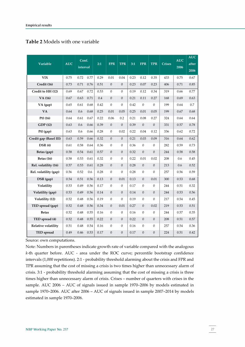
25
in section 3 of our paper AUC equal to 0.5 means that signals are non-
informative. Their accuracy is the same as of signals generated by Bernoulli
distribution with probability . The upper confidence interval
for such AUC value is 0.55. Variables that exceed this value are considered
useful. This criterion is used to identify the variables characterized by the
stability of accuracy. It is assumed that the accuracy of signals is stable when
in full, pre-crisis sample and out-of-sample exercise AUC is significantly
higher than 0.5. Thanks to that we filter out variables that are either non-
informative or their interpretation changes with time.
Results of stability check can be found in the last two columns of table 2. In
column ‘AUC before 2006’ we report accuracy of signals issued by models
that are estimated in pre-crisis sample. High value of AUC means that given
variable is useful predictor of banking crises in period 1970–2006. Last column
of table 2 informs how accurate are signals that are issued by those models in
period 2007–2014.
Even though in shorter, pre-crisis sample models generate equally accurate
signals as in full sample, in case of out-of-sample exercise for some variables
signals are statistically worse than in case of full of shorter sample. These
variables are VIX, level and growth rate of betas, volatility of banking sector
index and relative volatility of banking sector index. Thus, usefulness of VIX
is to some extent statistical artefact related with the global nature of the last
crisis that occurred in more than thirty countries in sample. Nonetheless VIX
still issues quite accurate signals. Furthermore VIX meet criteria set before,
hence it is considered in the next stage.
26
Table 2 Models with one variable
Variable AUC Conf.
interval 2:1 FPR TPR 3:1 FPR TPR Crises
AUC
2006
AUC
after
2006
VIX 0.75 0.72 0.77 0.29 0.01 0.04 0.23 0.12 0.35 433 0.75 0.67
Credit (16) 0.73 0.71 0.76 0.51 0 0 0.23 0.07 0.23 406 0.71 0.85
Credit to HH (12) 0.69 0.67 0.72 0.53 0 0 0.19 0.12 0.34 319 0.66 0.77
VA (16) 0.67 0.63 0.71 0.4 0 0 0.21 0.11 0.27 168 0.69 0.63
VA (gap) 0.65 0.61 0.68 0.42 0 0 0.42 0 0 199 0.64 0.7
VA 0.64 0.6 0.68 0.25 0.01 0.05 0.25 0.01 0.05 199 0.67 0.68
PtI (16) 0.64 0.61 0.67 0.22 0.06 0.2 0.21 0.08 0.27 324 0.64 0.64
GDP (12) 0.63 0.6 0.66 0.39 0 0 0.39 0 0 331 0.57 0.78
PtI (gap) 0.63 0.6 0.66 0.28 0 0.02 0.22 0.04 0.12 336 0.62 0.72
Credit gap (Basel III) 0.63 0.59 0.66 0.32 0 0 0.21 0.03 0.09 316 0.64 0.62
DSR (4) 0.61 0.58 0.64 0.36 0 0 0.36 0 0 282 0.59 0.73
Betas (gap) 0.58 0.54 0.61 0.57 0 0 0.32 0 0 244 0.58 0.58
Betas (16) 0.58 0.53 0.61 0.32 0 0 0.22 0.01 0.02 208 0.6 0.45
Rel. volatility (16) 0.57 0.53 0.61 0.28 0 0 0.28 0 0 213 0.6 0.52
Rel. volatility (gap) 0.56 0.52 0.6 0.28 0 0 0.28 0 0 257 0.56 0.59
DSR (gap) 0.54 0.51 0.56 0.13 0 0.01 0.13 0 0.01 300 0.53 0.68
Volatility 0.53 0.49 0.56 0.17 0 0 0.17 0 0 244 0.51 0.32
Volatility (gap) 0.53 0.49 0.56 0.14 0 0 0.14 0 0 244 0.53 0.56
Volatility (12) 0.52 0.48 0.56 0.19 0 0 0.19 0 0 217 0.54 0.45
TED spread (gap) 0.52 0.48 0.56 0.34 0 0.01 0.27 0 0.02 219 0.53 0.51
Betas 0.52 0.48 0.55 0.16 0 0 0.16 0 0 244 0.57 0.35
TED spread (4) 0.52 0.48 0.55 0.22 0 0 0.22 0 0 208 0.51 0.57
Relative volatility 0.51 0.48 0.54 0.16 0 0 0.16 0 0 257 0.54 0.36
TED spread 0.49 0.46 0.53 0.17 0 0 0.17 0 0 224 0.51 0.42
Source: own computations. Note: Numbers in parentheses indicate growth rate of variable compared with the analogous k-th quarter before. AUC - area under the ROC curve; percentile bootstrap confidence intervals (1,000 repetitions). 2:1 - probability threshold alarming about the crisis and FPR and TPR assuming that the cost of missing a crisis is two times higher than unnecessary alarm of crisis. 3:1 - probability threshold alarming assuming that the cost of missing a crisis is three times higher than unnecessary alarm of crisis. Crises – number of quarters with crises in the sample. AUC 2006 – AUC of signals issued in sample 1970–2006 by models estimated in sample 1970–2006. AUC after 2006 – AUC of signals issued in sample 2007–2014 by models estimated in sample 1970–2006.
27NBP Working Paper No. 257
Empirical results

27
4.3 Models with credit gap and three explanatory
variables
In this step we estimate models with credit gap and three explanatory
variables (table 3). Even though we analysed models with two and three
explanatory variables we do not report them, as models with two variables
have statistically worse predictive power than models with three variables.
The problem with three variables, however, is that the credit gap (computed
according to Basel III) very rarely enters most accurate early warning models.
However, accordingly to ESRB Recommendation (2014) credit gap has to be
incorporated into the model. To comply with this, we included credit gap in
each model and then added one, two and three additional explanatory
variables. Finally we end up with models of four variables in total, which were
statistically better than models comprising of smaller number of variables.
Furthermore early warning models with five variables were not statistically
more accurate than model with four variables. Below we report results
concerning these models.
In case of early warning models with credit gap and three explanatory
variables we see that all these models include VIX. Each of these models is
statistically more useful than the model based solely on VIX and eight models
with the highest AUC do not differ significantly from each other in terms of
signals accuracy (all these models are reported in table 3). For given
preferences of avoiding type I and type II errors we observe lower variation
in the probability thresholds that inform about crises compared with the case
of models with just one variable – model thresholds generally range between
20 to 30%. Additionally we do not only observe increase in overall quality of
28
the models but also there is improvement in terms of lower instances when a
crisis is missed – i.e. TPR ranges between 50 to 70%. As a result simultaneous
use of more than one variable in the model does not only increase overall
accuracy, but crucially substantially increases TPR with only very mild
increases in FPR.
Table 3 Models with credit gap and three explanatory variables
Model AUC Confidence
interval 2:1 FPR TPR 3:1 FPR TPR Crises
Credit gap (Basel III), DSR (4),
PtI (16) & VIX 0.92 0.88 0.95 0.3 0.1 0.76 0.3 0.1 0.76 156
Credit gap (Basel III), Betas
(gap), DSR (4) & VIX 0.92 0.88 0.95 0.36 0.07 0.68 0.28 0.11 0.79 121
Credit gap (Basel III), PtI (gap),
DSR (4) & VIX 0.92 0.88 0.95 0.3 0.09 0.76 0.3 0.09 0.76 156
Credit gap (Basel III), VA (gap),
DSR (4) & VIX 0.92 0.88 0.95 0.28 0.1 0.75 0.27 0.11 0.76 96
Credit gap (Basel III), VA, DSR
(4) & VIX 0.91 0.87 0.94 0.37 0.07 0.63 0.22 0.14 0.8 96
Credit gap (Basel III), VA (16),
DSR (4) & VIX 0.91 0.87 0.94 0.34 0.09 0.68 0.24 0.15 0.79 96
Credit gap (Basel III), Credit to
HH (12), DSR (4) & VIX 0.9 0.85 0.93 0.26 0.11 0.72 0.26 0.11 0.72 155
Credit gap (Basel III), DSR (4),
Credit (16) & VIX 0.89 0.85 0.92 0.32 0.06 0.47 0.19 0.14 0.77 178
Source: own computations.
Note: Numbers in parentheses indicate growth rate of variable compared with the analogous
k-th quarter before. AUC - area under the ROC curve; percentile bootstrap confidence
intervals (1,000 repetitions). 2:1 - probability threshold alarming about the crisis and FPR and
TPR assuming that the cost of missing a crisis is two times higher than unnecessary alarm of
crisis. 3:1 - probability threshold alarming assuming that the cost of missing a crisis is three
times higher than unnecessary alarm of crisis. Crises– number of quarters with crises in the
sample.
Narodowy Bank Polski28
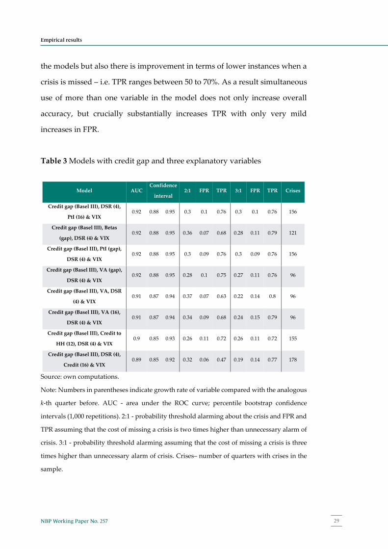
27
4.3 Models with credit gap and three explanatory
variables
In this step we estimate models with credit gap and three explanatory
variables (table 3). Even though we analysed models with two and three
explanatory variables we do not report them, as models with two variables
have statistically worse predictive power than models with three variables.
The problem with three variables, however, is that the credit gap (computed
according to Basel III) very rarely enters most accurate early warning models.
However, accordingly to ESRB Recommendation (2014) credit gap has to be
incorporated into the model. To comply with this, we included credit gap in
each model and then added one, two and three additional explanatory
variables. Finally we end up with models of four variables in total, which were
statistically better than models comprising of smaller number of variables.
Furthermore early warning models with five variables were not statistically
more accurate than model with four variables. Below we report results
concerning these models.
In case of early warning models with credit gap and three explanatory
variables we see that all these models include VIX. Each of these models is
statistically more useful than the model based solely on VIX and eight models
with the highest AUC do not differ significantly from each other in terms of
signals accuracy (all these models are reported in table 3). For given
preferences of avoiding type I and type II errors we observe lower variation
in the probability thresholds that inform about crises compared with the case
of models with just one variable – model thresholds generally range between
20 to 30%. Additionally we do not only observe increase in overall quality of
28
the models but also there is improvement in terms of lower instances when a
crisis is missed – i.e. TPR ranges between 50 to 70%. As a result simultaneous
use of more than one variable in the model does not only increase overall
accuracy, but crucially substantially increases TPR with only very mild
increases in FPR.
Table 3 Models with credit gap and three explanatory variables
Model AUC Confidence
interval 2:1 FPR TPR 3:1 FPR TPR Crises
Credit gap (Basel III), DSR (4),
PtI (16) & VIX 0.92 0.88 0.95 0.3 0.1 0.76 0.3 0.1 0.76 156
Credit gap (Basel III), Betas
(gap), DSR (4) & VIX 0.92 0.88 0.95 0.36 0.07 0.68 0.28 0.11 0.79 121
Credit gap (Basel III), PtI (gap),
DSR (4) & VIX 0.92 0.88 0.95 0.3 0.09 0.76 0.3 0.09 0.76 156
Credit gap (Basel III), VA (gap),
DSR (4) & VIX 0.92 0.88 0.95 0.28 0.1 0.75 0.27 0.11 0.76 96
Credit gap (Basel III), VA, DSR
(4) & VIX 0.91 0.87 0.94 0.37 0.07 0.63 0.22 0.14 0.8 96
Credit gap (Basel III), VA (16),
DSR (4) & VIX 0.91 0.87 0.94 0.34 0.09 0.68 0.24 0.15 0.79 96
Credit gap (Basel III), Credit to
HH (12), DSR (4) & VIX 0.9 0.85 0.93 0.26 0.11 0.72 0.26 0.11 0.72 155
Credit gap (Basel III), DSR (4),
Credit (16) & VIX 0.89 0.85 0.92 0.32 0.06 0.47 0.19 0.14 0.77 178
Source: own computations.
Note: Numbers in parentheses indicate growth rate of variable compared with the analogous
k-th quarter before. AUC - area under the ROC curve; percentile bootstrap confidence
intervals (1,000 repetitions). 2:1 - probability threshold alarming about the crisis and FPR and
TPR assuming that the cost of missing a crisis is two times higher than unnecessary alarm of
crisis. 3:1 - probability threshold alarming assuming that the cost of missing a crisis is three
times higher than unnecessary alarm of crisis. Crises– number of quarters with crises in the
sample.
29NBP Working Paper No. 257
Empirical results
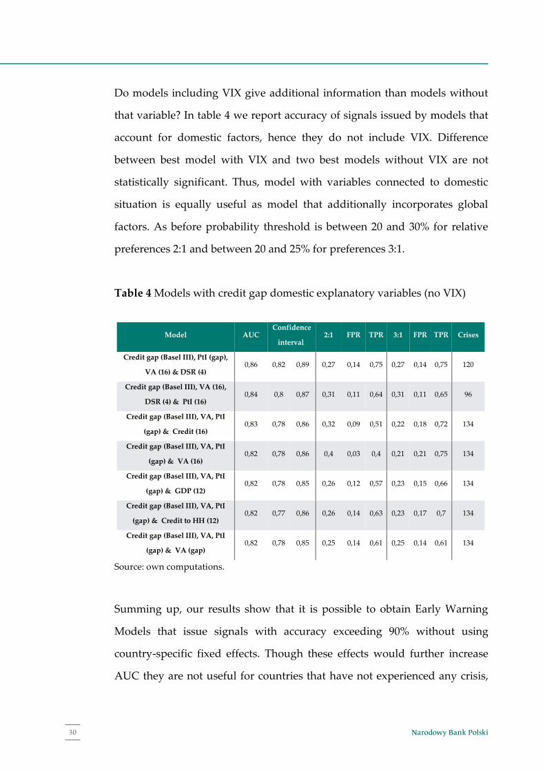
29
Do models including VIX give additional information than models without
that variable? In table 4 we report accuracy of signals issued by models that
account for domestic factors, hence they do not include VIX. Difference
between best model with VIX and two best models without VIX are not
statistically significant. Thus, model with variables connected to domestic
situation is equally useful as model that additionally incorporates global
factors. As before probability threshold is between 20 and 30% for relative
preferences 2:1 and between 20 and 25% for preferences 3:1.
Table 4 Models with credit gap domestic explanatory variables (no VIX)
Model AUC Confidence
interval 2:1 FPR TPR 3:1 FPR TPR Crises
Credit gap (Basel III), PtI (gap),
VA (16) & DSR (4) 0,86 0,82 0,89 0,27 0,14 0,75 0,27 0,14 0,75 120
Credit gap (Basel III), VA (16),
DSR (4) & PtI (16) 0,84 0,8 0,87 0,31 0,11 0,64 0,31 0,11 0,65 96
Credit gap (Basel III), VA, PtI
(gap) & Credit (16) 0,83 0,78 0,86 0,32 0,09 0,51 0,22 0,18 0,72 134
Credit gap (Basel III), VA, PtI
(gap) & VA (16) 0,82 0,78 0,86 0,4 0,03 0,4 0,21 0,21 0,75 134
Credit gap (Basel III), VA, PtI
(gap) & GDP (12) 0,82 0,78 0,85 0,26 0,12 0,57 0,23 0,15 0,66 134
Credit gap (Basel III), VA, PtI
(gap) & Credit to HH (12) 0,82 0,77 0,86 0,26 0,14 0,63 0,23 0,17 0,7 134
Credit gap (Basel III), VA, PtI
(gap) & VA (gap) 0,82 0,78 0,85 0,25 0,14 0,61 0,25 0,14 0,61 134
Source: own computations.
Summing up, our results show that it is possible to obtain Early Warning
Models that issue signals with accuracy exceeding 90% without using
country-specific fixed effects. Though these effects would further increase
AUC they are not useful for countries that have not experienced any crisis,
30
while models used in this study provide useful policy tools for both crisis and
non-crisis countries. Inclusion of VIX in models (a proxy for global factors) is
beneficial, however using data that reflects primarily domestic situation still
allows for high precision in issuing alarms.
Narodowy Bank Polski30

29
Do models including VIX give additional information than models without
that variable? In table 4 we report accuracy of signals issued by models that
account for domestic factors, hence they do not include VIX. Difference
between best model with VIX and two best models without VIX are not
statistically significant. Thus, model with variables connected to domestic
situation is equally useful as model that additionally incorporates global
factors. As before probability threshold is between 20 and 30% for relative
preferences 2:1 and between 20 and 25% for preferences 3:1.
Table 4 Models with credit gap domestic explanatory variables (no VIX)
Model AUC Confidence
interval 2:1 FPR TPR 3:1 FPR TPR Crises
Credit gap (Basel III), PtI (gap),
VA (16) & DSR (4) 0,86 0,82 0,89 0,27 0,14 0,75 0,27 0,14 0,75 120
Credit gap (Basel III), VA (16),
DSR (4) & PtI (16) 0,84 0,8 0,87 0,31 0,11 0,64 0,31 0,11 0,65 96
Credit gap (Basel III), VA, PtI
(gap) & Credit (16) 0,83 0,78 0,86 0,32 0,09 0,51 0,22 0,18 0,72 134
Credit gap (Basel III), VA, PtI
(gap) & VA (16) 0,82 0,78 0,86 0,4 0,03 0,4 0,21 0,21 0,75 134
Credit gap (Basel III), VA, PtI
(gap) & GDP (12) 0,82 0,78 0,85 0,26 0,12 0,57 0,23 0,15 0,66 134
Credit gap (Basel III), VA, PtI
(gap) & Credit to HH (12) 0,82 0,77 0,86 0,26 0,14 0,63 0,23 0,17 0,7 134
Credit gap (Basel III), VA, PtI
(gap) & VA (gap) 0,82 0,78 0,85 0,25 0,14 0,61 0,25 0,14 0,61 134
Source: own computations.
Summing up, our results show that it is possible to obtain Early Warning
Models that issue signals with accuracy exceeding 90% without using
country-specific fixed effects. Though these effects would further increase
AUC they are not useful for countries that have not experienced any crisis,
30
while models used in this study provide useful policy tools for both crisis and
non-crisis countries. Inclusion of VIX in models (a proxy for global factors) is
beneficial, however using data that reflects primarily domestic situation still
allows for high precision in issuing alarms.
31NBP Working Paper No. 257
Empirical results

31
5. Conclusions
The main goal of our study was to choose the variables whose behaviour
informs about the imminent banking crises that would be useful for both
countries that have experienced crises, and countries that have not. For this
purpose, we use early warning models based on logistic regression and
evaluate accuracy of signals with the ROC curve. Contrary to previous studies
we do not include country-specific fixed effects in model as this would result
in relatively low usefulness of models for countries that have not experienced
crises, nonetheless we implicitly take into account heterogeneity among
countries. To check the robustness of our results we also estimate probit and
scobit models as well as non-parametric approach. We analyse dozens of
indicators for nearly fifty countries and examine the stability of their signals.
We find that VIX, a proxy of price of risk on global financial market, is a
leading indicator, though its performance is partly due to global character of
the recent crisis. Still, low levels of VIX tended to precede crises even before
2006 and this is in line with Minsky’s hypothesis. Credit growth and property
prices enjoy among the highest predictive quality of signals, but we also find
that high growth in value added of the financial sector consistently predicts
crises. This is supportive to the hypothesis that unusually high profits in the
financial sector tend to reflect high risk, rather than high value added of its
products. Overall we find that using models with three variables exhibit AUC
above 90% and True Positive Rate over 70%, which is substantially more
compared to any single variable model.
32
References
Alessandri, P., Bologna, P., Fiori, R., & Sette, E. (2015). A note on the
implementation of the countercyclical capital buffer in Italy. Bank of Italy
Occasional Paper, (278).
Alessi, L., & Detken, C. (2011). Quasi real time early warning indicators for
costly asset price boom/bust cycles: A role for global liquidity. European
Journal of Political Economy, 27(3), 520-533.
Babecký, J., Havránek, T., Matějů, J., Rusnák, M., Šmídková, K., & Vašíček, B.
(2013). Leading indicators of crisis incidence: Evidence from developed
countries. Journal of International Money and Finance, 35, 1-19.
Basel Committee on Banking Supervision, Guidance for national authorities
operating the countercyclical capital buffer, 2010, Basel, Switzerland
Behn, M., Detken, C., Peltonen, T. A., & Schudel, W. (2013). Setting
countercyclical capital buffers based on early warning models: would it work?
ECB Working Paper No. 1604.
Borio, C. E., & Drehmann, M. (2009). Assessing the risk of banking crises–
revisited. BIS Quarterly Review, March.
Bussiere, M., & Fratzscher, M. (2006). Towards a new early warning system of
financial crises. journal of International Money and Finance, 25(6), 953-973.
Catão, L. A., & Milesi-Ferretti, G. M. (2014). External liabilities and crises.
Journal of International Economics, 94(1), 18-32.
Narodowy Bank Polski32
Chapter 5

31
5. Conclusions
The main goal of our study was to choose the variables whose behaviour
informs about the imminent banking crises that would be useful for both
countries that have experienced crises, and countries that have not. For this
purpose, we use early warning models based on logistic regression and
evaluate accuracy of signals with the ROC curve. Contrary to previous studies
we do not include country-specific fixed effects in model as this would result
in relatively low usefulness of models for countries that have not experienced
crises, nonetheless we implicitly take into account heterogeneity among
countries. To check the robustness of our results we also estimate probit and
scobit models as well as non-parametric approach. We analyse dozens of
indicators for nearly fifty countries and examine the stability of their signals.
We find that VIX, a proxy of price of risk on global financial market, is a
leading indicator, though its performance is partly due to global character of
the recent crisis. Still, low levels of VIX tended to precede crises even before
2006 and this is in line with Minsky’s hypothesis. Credit growth and property
prices enjoy among the highest predictive quality of signals, but we also find
that high growth in value added of the financial sector consistently predicts
crises. This is supportive to the hypothesis that unusually high profits in the
financial sector tend to reflect high risk, rather than high value added of its
products. Overall we find that using models with three variables exhibit AUC
above 90% and True Positive Rate over 70%, which is substantially more
compared to any single variable model.
32
References
Alessandri, P., Bologna, P., Fiori, R., & Sette, E. (2015). A note on the
implementation of the countercyclical capital buffer in Italy. Bank of Italy
Occasional Paper, (278).
Alessi, L., & Detken, C. (2011). Quasi real time early warning indicators for
costly asset price boom/bust cycles: A role for global liquidity. European
Journal of Political Economy, 27(3), 520-533.
Babecký, J., Havránek, T., Matějů, J., Rusnák, M., Šmídková, K., & Vašíček, B.
(2013). Leading indicators of crisis incidence: Evidence from developed
countries. Journal of International Money and Finance, 35, 1-19.
Basel Committee on Banking Supervision, Guidance for national authorities
operating the countercyclical capital buffer, 2010, Basel, Switzerland
Behn, M., Detken, C., Peltonen, T. A., & Schudel, W. (2013). Setting
countercyclical capital buffers based on early warning models: would it work?
ECB Working Paper No. 1604.
Borio, C. E., & Drehmann, M. (2009). Assessing the risk of banking crises–
revisited. BIS Quarterly Review, March.
Bussiere, M., & Fratzscher, M. (2006). Towards a new early warning system of
financial crises. journal of International Money and Finance, 25(6), 953-973.
Catão, L. A., & Milesi-Ferretti, G. M. (2014). External liabilities and crises.
Journal of International Economics, 94(1), 18-32.
33NBP Working Paper No. 257
References

33
Cecchetti, S. G., Kohler, M., & Upper, C. (2009). Financial crises and economic
activity (No. w15379). National Bureau of Economic Research. Davis, E. P., &
Karim, D. (2008). Comparing early warning systems for banking crises.
Journal of Financial stability, 4(2), 89-120.
Dekten C., O. Weeken, L. Alessi, D. Bonfim, M.M. Boucinha, C. Castro, S.
Frontczak, G. Giordana, J. Giese, N. Jahn, J. Kakes, B. Klaus, J.H. Lang, N.
Puzanova, P. Welz, 2014. Operationalising the countercyclical capital buffer:
indicator selection, threshold identification and calibration options,
Occasional Paper Series 5, European Systemic Risk Board
Drehmann, M., Borio, C., Gambacorta, L., Jiménez, G., & Trucharte, C. (2010).
Countercyclical capital buffers; exploring options (No. 317). BIS Working
Paper.
Drehmann, M., Borio, C. and Tsatsaronis, K.: 2012, Characterising the
financial cycle: don’t lose sight of the medium term!, BIS Working Papers No.
380.
Drehmann, M., & Juselius, M. (2012). Do debt service costs affect
macroeconomic and financial stability?. BIS Quarterly Review September.
Drehmann, M., & Juselius, M. (2014). Evaluating early warning indicators of
banking crises: Satisfying policy requirements. International Journal of
Forecasting, 30(3), 759-780
ESRB, Recommendation of the European Systemic Risk Board of 18 June 2014
on guidance for setting countercyclical buffer rates (ESRB/2014/1)
34
Gerdrup, K., Kvinlog, A., & Schaanning, E. (2013). Key indicators for a
countercyclical capital buffer in Norway–trends and uncertainty. Central
Bank of Norway (Norges Bank), Staff Memo, (13).
Haldane, A., Brennan, S., & Madouros, V. (2010). What is the contribution of
the financial sector: Miracle or mirage?. The Future of Finance, 87.
Hamilton, J. D. (1994). Time series analysis (Vol. 2). Princeton: Princeton
University Press.
Hodrick, R. J., & Prescott, E. C. (1997). Postwar US business cycles: an
empirical investigation. Journal of Money, credit, and Banking, 1-16.
Juks, R., & Melander, O. (2012). Countercyclical capital buffers as a
macroprudential instrument. Riksbank Studies.
Kaminsky, G. L., & Reinhart, C. M. (1999). The twin crises: the causes of
banking and balance-of-payments problems. American Economic Review,
473-500.
Lainà, P., Nyholm, J., & Sarlin, P. (2015). Leading indicators of systemic
banking crises: Finland in a panel of EU countries. Review of Financial
Economics, 24, 18-35.
Maravall, A., & Del Río, A. (2001). Time aggregation and the Hodrick-Prescott
filter (No. 0108). Banco de España.
Narodowy Bank Polski34

33
Cecchetti, S. G., Kohler, M., & Upper, C. (2009). Financial crises and economic
activity (No. w15379). National Bureau of Economic Research. Davis, E. P., &
Karim, D. (2008). Comparing early warning systems for banking crises.
Journal of Financial stability, 4(2), 89-120.
Dekten C., O. Weeken, L. Alessi, D. Bonfim, M.M. Boucinha, C. Castro, S.
Frontczak, G. Giordana, J. Giese, N. Jahn, J. Kakes, B. Klaus, J.H. Lang, N.
Puzanova, P. Welz, 2014. Operationalising the countercyclical capital buffer:
indicator selection, threshold identification and calibration options,
Occasional Paper Series 5, European Systemic Risk Board
Drehmann, M., Borio, C., Gambacorta, L., Jiménez, G., & Trucharte, C. (2010).
Countercyclical capital buffers; exploring options (No. 317). BIS Working
Paper.
Drehmann, M., Borio, C. and Tsatsaronis, K.: 2012, Characterising the
financial cycle: don’t lose sight of the medium term!, BIS Working Papers No.
380.
Drehmann, M., & Juselius, M. (2012). Do debt service costs affect
macroeconomic and financial stability?. BIS Quarterly Review September.
Drehmann, M., & Juselius, M. (2014). Evaluating early warning indicators of
banking crises: Satisfying policy requirements. International Journal of
Forecasting, 30(3), 759-780
ESRB, Recommendation of the European Systemic Risk Board of 18 June 2014
on guidance for setting countercyclical buffer rates (ESRB/2014/1)
34
Gerdrup, K., Kvinlog, A., & Schaanning, E. (2013). Key indicators for a
countercyclical capital buffer in Norway–trends and uncertainty. Central
Bank of Norway (Norges Bank), Staff Memo, (13).
Haldane, A., Brennan, S., & Madouros, V. (2010). What is the contribution of
the financial sector: Miracle or mirage?. The Future of Finance, 87.
Hamilton, J. D. (1994). Time series analysis (Vol. 2). Princeton: Princeton
University Press.
Hodrick, R. J., & Prescott, E. C. (1997). Postwar US business cycles: an
empirical investigation. Journal of Money, credit, and Banking, 1-16.
Juks, R., & Melander, O. (2012). Countercyclical capital buffers as a
macroprudential instrument. Riksbank Studies.
Kaminsky, G. L., & Reinhart, C. M. (1999). The twin crises: the causes of
banking and balance-of-payments problems. American Economic Review,
473-500.
Lainà, P., Nyholm, J., & Sarlin, P. (2015). Leading indicators of systemic
banking crises: Finland in a panel of EU countries. Review of Financial
Economics, 24, 18-35.
Maravall, A., & Del Río, A. (2001). Time aggregation and the Hodrick-Prescott
filter (No. 0108). Banco de España.
35NBP Working Paper No. 257
References

35
Ravn, M. O., & Uhlig, H. (2002). On adjusting the Hodrick-Prescott filter for
the frequency of observations. Review of economics and statistics, 84(2), 371-
376.
Schüler, Y. S., Hiebert, P. P., & Peltonen, T. A. (2015). Characterising the
financial cycle: A multivariate and time-varying approach. ECB Working
Paper No. 1846.
Wang C., What is the value added of banks?, VOX CEPR’s policy portal,
08.12.2011
36
Appendix A Data description and sources
List of variables and sources:
Credit extended to non-financial sector; credit extended to households
– BIS.
Nominal GDP – Eurostat.
Debt service ratio (DSR) – BIS.
Residential property prices relative to income – OECD.
VIX - Datastream
Banking sector index beta – Datastream (Thomson Reuters).
Volatility of banking sector index – Datastream (Thomson Reuters).
Contribution of banking sector to GDP growth – Datastream (Thomson
Reuters).
TED spread – Datastream (Thomson Reuters).
Volatility of banking sector index relative to market volatility –
Datastream (Thomson Reuters).
Nominal variables were deflated with CPI (OECD).
Narodowy Bank Polski36

35
Ravn, M. O., & Uhlig, H. (2002). On adjusting the Hodrick-Prescott filter for
the frequency of observations. Review of economics and statistics, 84(2), 371-
376.
Schüler, Y. S., Hiebert, P. P., & Peltonen, T. A. (2015). Characterising the
financial cycle: A multivariate and time-varying approach. ECB Working
Paper No. 1846.
Wang C., What is the value added of banks?, VOX CEPR’s policy portal,
08.12.2011
36
Appendix A Data description and sources
List of variables and sources:
Credit extended to non-financial sector; credit extended to households
– BIS.
Nominal GDP – Eurostat.
Debt service ratio (DSR) – BIS.
Residential property prices relative to income – OECD.
VIX - Datastream
Banking sector index beta – Datastream (Thomson Reuters).
Volatility of banking sector index – Datastream (Thomson Reuters).
Contribution of banking sector to GDP growth – Datastream (Thomson
Reuters).
TED spread – Datastream (Thomson Reuters).
Volatility of banking sector index relative to market volatility –
Datastream (Thomson Reuters).
Nominal variables were deflated with CPI (OECD).
37NBP Working Paper No. 257
Appendix A

37
Appendix B Logistic regression models
Table 5 Summary of the best models
Model 1 Model 2 Model 3 Model 4 Model 5 Model 6
Constant -2.594*** -2.324*** -3.094*** -1.382*** -4.135*** -1.351***
-0.082 (0.063) (0.135) (0.141) (0.293) (0.170)
VIX -1.400*** -2.004*** -3.471***
-0.103 (0.161) (0.321)
Credit (16) 0.774***
(0.054)
DSR (4) 0.675*** 0.634*** 0.215
(0.087) (0.133) (0.131)
Banks contribution to
GDP (16)
0.009*** 0.011***
(0.001) (0.001)
Property price to income
(16)
0.028*** 0.035*** 0.030***
(0.004) (0.004) (0.005)
Sample 3813 3702 2402 829 1103 576
Model p-value 0.000 0.000 0.000 0.000 0.000 0.000
AUC 0.746 0.729 0.828 0.797 0.912 0.859
Source: own computations.
Note: *** - variable significant at 1% significance level.; standard errors are reported in
parentheses; model p-value– p-value of the test, whose null hypothesis assumes no difference
between analyzed model and model without any explanatory variables (only with constant).
38
Appendix C ROC curves
Figure 3 shows ROC curve for models with the highest AUC analysed in part
4 and percentile bootstrap confidence intervals (1,000 repetitions). Red circle
– costs of errors 2:1, blue circle – costs 3:1.
Figure 3 ROC curves
Source: own computations.
Note: Description of models can be found in appendix B.
Narodowy Bank Polski38
Appendix B

37
Appendix B Logistic regression models
Table 5 Summary of the best models
Model 1 Model 2 Model 3 Model 4 Model 5 Model 6
Constant -2.594*** -2.324*** -3.094*** -1.382*** -4.135*** -1.351***
-0.082 (0.063) (0.135) (0.141) (0.293) (0.170)
VIX -1.400*** -2.004*** -3.471***
-0.103 (0.161) (0.321)
Credit (16) 0.774***
(0.054)
DSR (4) 0.675*** 0.634*** 0.215
(0.087) (0.133) (0.131)
Banks contribution to
GDP (16)
0.009*** 0.011***
(0.001) (0.001)
Property price to income
(16)
0.028*** 0.035*** 0.030***
(0.004) (0.004) (0.005)
Sample 3813 3702 2402 829 1103 576
Model p-value 0.000 0.000 0.000 0.000 0.000 0.000
AUC 0.746 0.729 0.828 0.797 0.912 0.859
Source: own computations.
Note: *** - variable significant at 1% significance level.; standard errors are reported in
parentheses; model p-value– p-value of the test, whose null hypothesis assumes no difference
between analyzed model and model without any explanatory variables (only with constant).
38
Appendix C ROC curves
Figure 3 shows ROC curve for models with the highest AUC analysed in part
4 and percentile bootstrap confidence intervals (1,000 repetitions). Red circle
– costs of errors 2:1, blue circle – costs 3:1.
Figure 3 ROC curves
Source: own computations.
Note: Description of models can be found in appendix B.
39NBP Working Paper No. 257
Appendix C

www.nbp.pl


![The following table lists ICICI Bank’s financial and non...Sep 30, 2020 · [India] Yes Accounted as per AS 23 No Not applicable Not applicable This is a non-financial entity and](https://cdn.vdocuments.us/doc/165x107/611df3a22340b5255074a0e5/the-following-table-lists-icici-bankas-financial-and-non-sep-30-2020-india.jpg)

![OAK RIDGE ENVIRONMENTAL MANAGEMENT - … · Web viewREPRESENTATIONS, CERTIFICATIONS AND OTHER STATEMENTS OF OFFERORS (APPLICABLE FOR NON-COMMERCIAL) [PN: NON-COMMERCIAL OVER $10K]](https://cdn.vdocuments.us/doc/165x107/5ac9ae077f8b9aa1298d3f5c/oak-ridge-environmental-management-viewrepresentations-certifications-and.jpg)

