Download - Ea 10 07 Osciloscopios

8/3/2019 Ea 10 07 Osciloscopios
http://slidepdf.com/reader/full/ea-10-07-osciloscopios 1/29
EDITION 1 ® JUNE 1997 EA-10/07 PAGE 1 OF 29
European cooperation for
Accreditation of Laboratories
Publication Reference EAL-G30
Calibration of Oscilloscopes
PURPOSE
This document has been produced by EAL to harmonise oscilloscope calibration. It providesguidance to national accreditation bodies in setting up minimum requirements for the calibration ofoscilloscopes and gives advice to calibration laboratories to establish practical procedures.
8/3/2019 Ea 10 07 Osciloscopios
http://slidepdf.com/reader/full/ea-10-07-osciloscopios 2/29
EAL-G30 - CALIBRATION OF OSCILLOSCOPES
EDITION 1 ® JUNE 1997 EA-10/07 PAGE 2 OF 29
Authorship
This document has been revised by EAL Committee 2 (Calibration and Testing Activities), basedon the draft produced by the EAL Expert Group "DC and LF Electrical Quantities".
Official language The text may be translated into other languages as required. The English language versionremains the definitive version.
Copyright
The copyright of this text is held by EAL. The text may not be copied for resale.
Guidance Publications
This document represents a consensus of EAL member opinion and preferred practice on how therelevant clauses of the accreditation standards might be applied in the context of the subject matterof this document. The approaches taken are not mandatory and are for the guidance ofaccreditation bodies and their client laboratories. Nevertheless, the document has been produced
as a means of promoting a consistent approach to laboratory accreditation amongst EAL memberbodies, particularly those participating in the EAL Multilateral Agreement.
Further information
For further information about this publication, contact your National member of EAL:
Calibration National member Testing National member
Austria BMwA BMwA
Belgium BKO/OBE BELTEST
Denmark DANAK DANAK
Finland FINAS FINAS
France COFRAC COFRACGermany DKD DAR
Greece ESYD ESYD
Iceland ISAC ISAC
Italy SIT SINAL
Netherlands RvA RvA
Norway NA NA
Portugal IPQ IPQ
Spain ENAC ENAC
Sweden SWEDAC SWEDAC
Switzerland SAS SAS
United Kingdom UKAS UKAS

8/3/2019 Ea 10 07 Osciloscopios
http://slidepdf.com/reader/full/ea-10-07-osciloscopios 3/29
EAL-G30 - CALIBRATION OF OSCILLOSCOPES
EDITION 1 ® JUNE 1997 EA-10/07 PAGE 3 OF 29
Contents
Section Page
1 Introduction 4
2 Scope 4
3 Terms and abbreviations 4
4 Calibration equipment 5
5 Preparation for calibration 6
6 Calibration 6
7 Calibration Certificates 17
8 References 18
Appendix A 19

8/3/2019 Ea 10 07 Osciloscopios
http://slidepdf.com/reader/full/ea-10-07-osciloscopios 4/29
EAL-G30 - CALIBRATION OF OSCILLOSCOPES
EDITION 1 ® JUNE 1997 EA-10/07 PAGE 4 OF 29
1 Introduction
1.1 This document deals with the calibration of oscilloscopes. It does not claim to fullycover all metrological details of oscilloscopes even if important for calibration. In
this document, relevant standards and publications (cf. section 8) have been
allowed for. In addition, the manufacturer's data for the oscilloscope in question
should be taken into account for the calibration.
2 Scope of application of the calibration
2.1 This document applies to the calibration of electron-beam oscilloscopes and here to
both analogue oscilloscopes and digital storage oscilloscopes, and transient
recorders.
2.2 When the calibration is carried out, the measurement procedures applied by the
calibration laboratories shall be employed in conjunction with the calibration
equipment such that all measurands necessary for calibration are traceable on the
basis of the laboratory's accreditation for the calibration of oscilloscopes. The
traceability to national standards as well as the basic measurement procedures for
the calibration of oscilloscopes shall be documented.
3 Terms and abbreviations
Terms
B bandwidth
b correction factor
GL
input conductance of the power meter
GOS
conductance at the oscilloscope input
L linearity of the time base
n number of averaged curves
P power of the generator
Pinc incident power to a load
t i, t
i-1times
t o
rise time of the oscilloscope
T p period
T piperiod for the i-th time interval
Û peak voltage

8/3/2019 Ea 10 07 Osciloscopios
http://slidepdf.com/reader/full/ea-10-07-osciloscopios 5/29
EAL-G30 - CALIBRATION OF OSCILLOSCOPES
EDITION 1 ® JUNE 1997 EA-10/07 PAGE 5 OF 29
U E
voltage at the output
U IN
voltage at the input
Z 0 reference characteristic impedance Z
Ximpedance
Γ reflection coefficient
ϕ phase error
Abbreviations
AO analogue oscilloscope
DSO digital storage oscilloscope
SNR signal-to-noise ratio
4 Calibration equipment
4.1 Requirements to be met by calibration equipment
4.1.1 The calibration shall be carried out using measuring equipment and procedures
enabling relative uncertainties of measurement which are small compared with the
relative uncertainties of measuring for the oscilloscope.
4.1.2 Rise and decay times of rectangular calibration signals shall be significantly shorter
than the rise times of the oscilloscope under consideration.
4.1.3 Connecting cables shall be of the coaxial type. It shall be ensured that, for high-
frequency (HF) measurements, the output impedance of the measuring set-up and
the input impedance of the oscilloscope are matched to one another.
4.2 Reference conditions
4.2.1 The calibration shall be carried out under the reference conditions (e.g. ambient
temperature, humidity, voltage supply, harmonic distortion) specified for the
oscilloscope and the measuring equipment. During calibration, the measuring set-
up shall be in thermal equilibrium. The warm-up times specified by the
manufacturers shall be complied with.

8/3/2019 Ea 10 07 Osciloscopios
http://slidepdf.com/reader/full/ea-10-07-osciloscopios 6/29
EAL-G30 - CALIBRATION OF OSCILLOSCOPES
EDITION 1 ® JUNE 1997 EA-10/07 PAGE 6 OF 29
5 Preparation for calibration
5.1 Visual inspection
5.1.1 Prior to calibration, the general external condition of the oscilloscope shall be
checked. Defects which might inadmissibly affect the function shall be eliminated
before carrying out the calibration.
5.2 Functional test
5.2.2 The equipment to be calibrated shall be checked for correct operation, i. e. the
trigger sensitivity.
6 Calibration
6.1 Design criteria of an oscilloscope
6.1.1 The oscilloscope is a measuring instrument important for displaying physical
relations of a function
y = f(x ) (1)
where a physical quantity transformed into an electrical signal can be shown on theY-axis. The X-axis is a time function, but it can also correspond to another physical
quantity. The oscilloscope is suitable for analysing DC, AC voltages, and AC
voltages with DC components.
6.1.2 The design of an oscilloscope always comprises
• a vertical system,
• a horizontal system, and
• a visual display unit.

8/3/2019 Ea 10 07 Osciloscopios
http://slidepdf.com/reader/full/ea-10-07-osciloscopios 7/29
EAL-G30 - CALIBRATION OF OSCILLOSCOPES
EDITION 1 ® JUNE 1997 EA-10/07 PAGE 7 OF 29
Tab. 1 shows the relations between the design of an oscilloscope and some
associated important criteria.
Tab. 1 Construction and design criteria of an oscilloscope
Oscilloscope
Vertical system Horizontal system Visual display unit
Construction Criteria Construction Criteria Criteria
input divider bandwidth trigger linearity beam brightness
rise time time base accuracy
preamplifier sensitivity sensitivity sensitivity
delay line pulse response bandwidth
output amplifier ripple
A/D conversion resolution focusing
external divider linearity geometric distortion
6.2 Scope of calibration of an oscilloscope
6.2.1 The calibration covers
• vertical deflection,
• horizontal deflection,
• rise time and bandwidth, respectively,
• internal calibration signals, as far as an internal calibration signal
is available on the front panel.
6.2.2 If the plug-in units of plug-in oscilloscopes are of the replaceable type, it will be
necessary to separately calibrate individual configurations. Connected probe heads
shall be covered by the calibration. For all calibrations, elements for adjusting
deflection coefficients shall be in the defined positions.
6.2.3 When calibrations are carried out, the information given in Appendix A for the
acquisition of measured data shall be considered. An uncertainty budget of the
calibration procedures shall be documented in the quality manual. The centre line
of the beam shall be used for the evaluation of signals. For digital storage
oscilloscopes, it is recommended to take the mean of several recordings to reduce
the influence of digitisation.

8/3/2019 Ea 10 07 Osciloscopios
http://slidepdf.com/reader/full/ea-10-07-osciloscopios 8/29
EAL-G30 - CALIBRATION OF OSCILLOSCOPES
EDITION 1 ® JUNE 1997 EA-10/07 PAGE 8 OF 29
6.3 Calibration of the vertical deflection (amplitude calibration)
6.3.1 Carrying-out of the calibration
6.3.1.1 For calibrating the vertical deflection, any of the following items can be used:
• DC voltage,
• chopped DC voltage,
• AC voltage, or
• pulses.
The amplitude shall be measured in the linear range of the amplitude/frequency
characteristic of the oscilloscopes (cf. Fig. 6, see p. 27). It is recommended to use arepetition frequency between 1 kHz and 100 kHz. For digital storage oscilloscopes
(DSO), the measurement values should be recorded using ≥80 % of the grid
(Fig. 1), but for analogue oscilloscopes (AO) about 70 % should be used. The
operating ranges specified by the manufacturer shall be allowed for.
Fig. 1: Calibration of the vertical deflection of digital storageoscilloscopes
6.3.1.2 The calibration shall be carried out in each position of the voltage divider. If the
input divider sensitivity is multiplied by a fixed factor (e.g. x 10), the additional
deviation due to the multiplication shall be determined. In the case of multi-channel
systems, the measurements shall be identified by the channel number. The
calibration of the divider in a probe connected to an oscilloscope is valid only for
the calibrated oscilloscope (specified in the calibration certificate). The calibration
of the divider in a probe shall be unambiguously assigned to a channel. The divider
probe shall be identified in the calibration certificate.

8/3/2019 Ea 10 07 Osciloscopios
http://slidepdf.com/reader/full/ea-10-07-osciloscopios 9/29
EAL-G30 - CALIBRATION OF OSCILLOSCOPES
EDITION 1 ® JUNE 1997 EA-10/07 PAGE 9 OF 29
6.3.1.3 Table 2 gives an overview of the potential variants of traceability for the calibration
of the vertical deflection of an oscilloscope. The variants of Table 2 are described
in the text below.
Tab. 2: Variants of traceability for the calibration of vertical deflection
Variant Standard procedure Reference standard Working standard
1 Accreditation forDC voltage
Digital voltmeter Oscilloscopecalibrator
2 Accreditation forAC voltage
AC calibrator
3 Accreditation forpulse measurement
Pulse generator
6.3.2 Variant I: Accreditation for DC voltage (Fig. 2)
6.3.2.1 The calibration of the vertical deflection is traceable through the measurand DCvoltage. As a prerequisite, the laboratory shall be accredited for the measurand DC
voltage with a sufficiently small uncertainty of measurement. A digital voltmeter or
a DC calibrator can be used as a reference standard to calibrate the amplitude
generator. Oscilloscopes are calibrated in the "chopped" mode of the amplitude
calibrator. The uncertainty of measurement produced by the transition from the DC
mode to the chopped mode shall be taken into account.
Fig. 2: Traceability through using the measurand DC voltage
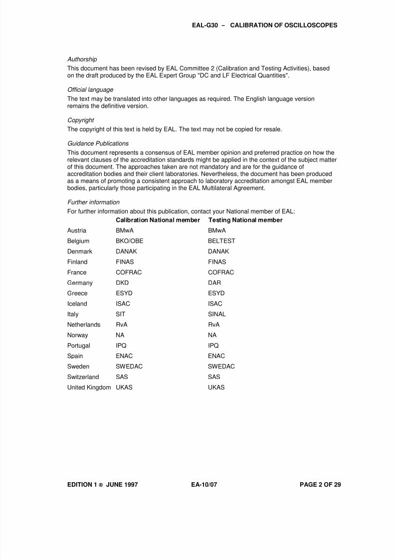
6.3.3 Variant II: Accreditation for AC voltage (Fig. 3)
6.3.3.1 The calibration is traceable through using the measurand AC voltage. The
calibration laboratory holds the accreditation for this measurand. The reference
standard can be an AC calibrator or a digital voltmeter. The working standard is
Accreditation for DC voltage Digital voltmeter/DC calibrator
Amplitude generator
Oscilloscope
8/3/2019 Ea 10 07 Osciloscopios
http://slidepdf.com/reader/full/ea-10-07-osciloscopios 10/29

8/3/2019 Ea 10 07 Osciloscopios
http://slidepdf.com/reader/full/ea-10-07-osciloscopios 11/29
EAL-G30 - CALIBRATION OF OSCILLOSCOPES
EDITION 1 ® JUNE 1997 EA-10/07 PAGE 11 OF 29
6.4 Calibration of the horizontal deflection (time base calibration)
6.4.1 Time base calibration
6.4.4.1 The sweep generator shall furnish the correct deflection voltage (linear with time)in the whole frequency range up to 10 decades (cf. Appendix A). For each coarse
range, only one setting point arbitrarily defined is regarded as calibrated. Expansion
factors can be graded 1/2/5/10 or 1/3/10. A certain position of the fine controller
(left or right stop, mechanical stop point, priority code for incremental adjustment)
— often marked by LED or indication in the display — defines the nominal defined
deflection velocity. The range of control of the fine controller shall ensure
overlapping of the individual subranges which are of varying size, however, it is
not to be calibrated. The additional expansion (switch-over of amplification) by the
factor 5 or 10 shall be calibrated. The calibration is carried out
• for analogue oscilloscopes: in all time ranges
• for digital storage oscilloscopes: in a mean sweep range
In the case of double time-base deflections (sweep), the two time bases shall be
measured independently of each other, each in the fine controller position marked
as calibrated.
6.4.1.2 The phase deviation between the X and the Y channels shall be checked by
simultaneously displaying the same sinusoidal measurement voltage through both
channels (Lissajous figures). Correct branching shall be performed by power
dividers (matching) with measurement cables of equal length between powerdivider and input connector (same delay). Simple reversing of X and Y connections
and checking that the result does not change indicates whether any phase deviations
have been introduced. The calibration shall be carried out at the nominal cut-off
frequency of the oscilloscope and at half this value (or as agreed with the
customer).
6.4.2 Calibration procedure
6.4.2.1 Calibration signals can be arbitrary periodic signals of sufficient stability and
accuracy. The use of signals in pulse form, which are obtained by phase-lockedfrequency division from a traceable basic cycle, should be preferred. These should,
ideally, have a well-defined edge to ease alignment with graticule marks.
6.4.2.2 This allows quartz oscillators to be used as pulse rate generators which have been
made traceable by repeated calibration or synchronisation with a local frequency
standard controlled by a radio transmitter, a television transmitter or other
procedures (Fig. 5, see p. 12).

8/3/2019 Ea 10 07 Osciloscopios
http://slidepdf.com/reader/full/ea-10-07-osciloscopios 12/29

8/3/2019 Ea 10 07 Osciloscopios
http://slidepdf.com/reader/full/ea-10-07-osciloscopios 13/29
EAL-G30 - CALIBRATION OF OSCILLOSCOPES
EDITION 1 ® JUNE 1997 EA-10/07 PAGE 13 OF 29
6.5 Determination of bandwidth and rise time
6.5.1 General
6.5.1.1 The frequency range within which the voltage amplitude response decreases by3 dB is referred to as the bandwidth B. The high-end cut-off frequency is the upper
limit of the bandwidth B (Fig. 6).
6.5.1.2 For time measurement, the rise time t o of the oscilloscope is of interest with which
an ideal voltage step is displayed on the screen. The rise time is measured on
voltage steps between the points in which the signal has reached 10 % and 90 %,
respectively, of the final value (Fig. 7).
Fig. 6: Frequency response
Fig. 7: Determination of the rise time

8/3/2019 Ea 10 07 Osciloscopios
http://slidepdf.com/reader/full/ea-10-07-osciloscopios 14/29

8/3/2019 Ea 10 07 Osciloscopios
http://slidepdf.com/reader/full/ea-10-07-osciloscopios 15/29
EAL-G30 - CALIBRATION OF OSCILLOSCOPES
EDITION 1 ® JUNE 1997 EA-10/07 PAGE 15 OF 29
Fig. 8: Basic circuit for amplitude measurements using a voltmeter
(c) The voltage to be measured is fed into the T junction from a variable-frequency
generator through the third connection (in the centre of T)(cf. Appendix A).When connected in parallel, calibrated HF power meters can be used instead of
voltmeters if their input impedance or admittance is known with sufficient
accuracy. Using a sinusoidal voltage as measurement signal, the amplitude or
the peak value Û of the voltage is obtained from the equation
Û = ( )2 P G / L (3)
withP effective power at the input of the calibrated power meter, andG
Linput conductance of the power meter.
(d) When the power meter impedance equals the characteristic impedance Z o of the
HF power system (in most cases 50 Ω), the well-known relation
Û = 2 0P Z (4)
applies. The reference plane of the voltage measurement using power meters is themeasurement plane of their input impedance or input admittance. The amplitudemeasurement with a T junction and a voltmeter (or power meter) can be used for
oscilloscopes with a high and low (50 Ω) input impedance.
(e) For high-impedance oscilloscopes, an alternative method without a T junction
is often used or specified by manufacturers. A generator with an output
impedance of 50 Ω is terminated with a matched 50 Ω load, and theoscilloscope is connected in parallel with this load. The bandwidth is
determined by the 3 dB roll-off of the voltage indicated by the oscilloscope.
Further instructions of the manufacturers concerning the measurement of
bandwidths shall be considered. Up to the highest frequency considered, the
impedance shall be significantly larger than 50 Ω, otherwise additional
uncertainties of measurement will be introduced.
Reference plane
Voltmeter Oscilloscope
Generator

8/3/2019 Ea 10 07 Osciloscopios
http://slidepdf.com/reader/full/ea-10-07-osciloscopios 16/29
EAL-G30 - CALIBRATION OF OSCILLOSCOPES
EDITION 1 ® JUNE 1997 EA-10/07 PAGE 16 OF 29
6.5.2.2 Amplitude measurements using a calibrated power generator
(a) In the frequency range above 1 GHz, accurate voltage measurements are
usually not carried out using a voltmeter connected in parallel with the aid of a
T junction. At these frequencies, amplitude or voltage measurements aretraceable to a power and impedance measurement (Fig. 9). For the amplitude
measurement using an HF power generator, this generator is first calibrated
using a calibrated power meter. The effective power P which the generator
feeds into the input of the oscilloscope during this measurement produces a
voltage with the peak value
Û = ( )2 P G / O S
(5)
G OS
being the conductance at the oscilloscope input (Fig. 9).
(b) The method shown in Fig. 9 can be modified by using a power splitter with the
power meter on one output port and the oscilloscope on the other output port,
thus improving (often considerably) the source match ( Γ G ). For a symmetrical
power splitter, Eq.(5) is valid.
Reference plane
Γ N Power meter
Generator Γ G
Γ OSOscilloscope
Fig. 9: Basic circuit for amplitude measurements using a powergenerator at high frequencies
(c) The voltage measurement described above concerns the HF voltage developedat the plane of the input connector of the oscilloscope. At higher frequencies,
especially above 1 GHz, an alternative method is often applied for bandwidth
measurements: The equipment described above with a matched power splitter
and with a calibrated power meter and the oscilloscope at its two output ports is
used. The power Pinc incident to the oscilloscope and obtained from the
measurement value of the calibrated power meter using its calibration factor is
determined. The amplitude of the incident voltage wave to the oscilloscope is
ascertained by calculating Û = ( )2 0P Z inc . The method applied shall be
mentioned in each bandwidth calibration.

8/3/2019 Ea 10 07 Osciloscopios
http://slidepdf.com/reader/full/ea-10-07-osciloscopios 17/29
EAL-G30 - CALIBRATION OF OSCILLOSCOPES
EDITION 1 ® JUNE 1997 EA-10/07 PAGE 17 OF 29
(d) When calibrated voltage or power generators are used, the bandwidth
measurement is traceable to AC and HF voltage standards or to HF power and
HF reflection standards. Eq. (5) will be valid only if the reflection coefficients
of the generator ( Γ G ), the power meter ( Γ N ) and the oscilloscope ( Γ OS ) are
negligibly small; otherwise the voltage Û shall be multiplied by a factor b. The
calculation of this factor is described in part A4 of the Appendix A.
6.6 Internal calibration signals
6.6.1 Amplitudes and frequencies of the internal calibration signals shall be calibrated in
accordance with sections 6.1 to 6.4. Such measurements often require special
techniques because internal calibration signals are often available as voltage (or
current) pulse form appearing at a test output on the front panel.
7 Calibration Certificates
7.1 In the calibration certificate, values shall be stated with reference to the conditions
and setting values relevant to the respective measurement. When parameter(s) are
certified to be within specified tolerances, the measurement value(s), extended by
the estimated uncertainty of measurement calculated in accordance with EAL-R2
[ref. 3], shall fall within the appropriate specification limit [ref. 2].

8/3/2019 Ea 10 07 Osciloscopios
http://slidepdf.com/reader/full/ea-10-07-osciloscopios 18/29
EAL-G30 - CALIBRATION OF OSCILLOSCOPES
EDITION 1 ® JUNE 1997 EA-10/07 PAGE 18 OF 29
8 References
1 IEC 351 part 1. Statement of the characteristics of electron beam oscilloscopes.November 1981
2 EAL-R1. Requirements concerning Certificates Issued by Accredited Calibration Laboratories. November 1995
3 EAL-R2. Expression of the Uncertainty of Measurement in Calibration. 1990
4 IEC 1083-1. Digital recorders for measurements in high-voltage impulse tests. Part 1: Requirements for digital recorders. 1991
5 Schuon, E. ; Wolf, H.: Nachrichtenmeßtechnik . Springer-Verlag Berlin, Heidelberg,
New York, 1981
6 Mellis, D.: Schnelle Speicheroszilloskope. Philips GmbH Kassel, 1989
7 Gans, W.: Dynamic calibration of oscillopes and waveform recorders. Conf.
Record of IEEE Instrum. Meas. Tech. Conf., San Jose, CA, Feb. 13-15, 1989
8 Green, P. J.: Automated test and evaluation center for waveform digitizer systemsand components. IEEE-IM 39 (1990)1, 101

8/3/2019 Ea 10 07 Osciloscopios
http://slidepdf.com/reader/full/ea-10-07-osciloscopios 19/29
EAL-G30 - CALIBRATION OF OSCILLOSCOPES
EDITION 1 ® JUNE 1997 EA-10/07 PAGE 19 OF 29
APPENDIX A
A1 Data output
A1.1 The oscilloscope is used for determining signal patterns as a function of time:
Y = f(t ) (A1)
Special transducers can be used to represent other physical quantities:
Y = f(X ) (A2)
A1.2 The measured data are indicated via the display screen or specific data interfaces.
The signals are adapted in their amplitude by means of amplifier/attenuator settings
(and, if necessary, by additional external dividers) and in the time axis by changingthe frequency of the deflection generator.
A1.3 To facilitate the interpretation of the wave form represented on the screen, the latter
is provided with a graticule whose units correspond to volts/division for the vertical
axis and to second/division for the horizontal axis. Superimposed alphanumeric
captions or cursor functions can be used to assist the characterisation of the display
(Fig. A1). With the digital storage oscilloscope, interfaces are available, which
provide access to the curve data for further signal processing (e.g. in a computer).
Fig. A1: Pulse representation on the display screen
A1.4 The graticule allows measurements of the amplitude, of the frequency and of the
signal rise to be performed and further signal characterizations to be made, such as

8/3/2019 Ea 10 07 Osciloscopios
http://slidepdf.com/reader/full/ea-10-07-osciloscopios 20/29
EAL-G30 - CALIBRATION OF OSCILLOSCOPES
EDITION 1 ® JUNE 1997 EA-10/07 PAGE 20 OF 29
those of the transient effects, the decay behaviour and the tilt distortions. Most
digital storage oscilloscopes have extended signal analysis capabilities such as
integration, differentiation and Fourier transformation and calculate the signal
parameters from the digitized data.
A2 Data evaluation
A2.1 Signal analysis by means of an oscilloscope is affected by uncertainties. The
uncertainties result from the oscilloscope used, from the signal adaptation and the
ratio between signal and oscilloscope parameters. In particular the bandwidth, the
rise times of the signal and the signal representation, line terminations, input and
output impedances as well as — in the case of the digital storage oscilloscope —
the scanning frequency and the type of scanning shall be allowed for.
A3 Uncertainties of measurement in oscilloscope
calibration
A3.1 Displaying system
A3.1.1 When the signal is analysed by using the screen, the raster type shall be taken into
account. A distinction is made between external and internal graticules. The
external graticule is applied to the cathode-ray tube from the front. The resulting
spacing between phosphor layer and raster is at least equal to the glass thickness
(according to the type). This gives rise to a parallactic uncertainty which can be
considerably minimized by the use of an internal graticule. This is engraved on the
inside glass face.
A3.1.2 Due to geometrical distortions of the beam deflection, only 60 % to 70 % of the
vertical central range of indication is often used. As a result of noise and since
focusing is limited, the beam width can be of the order of 1 % to 2 % of the range
of indication. The centre of the beam interpolated by the eye is used as a reference
point. With digital storage oscilloscopes provided with a graticule scan screen, the
graticule is electronically produced in one plane with the signal beam. In the case of
uncorrelated noise distributing the signal, the signal-to-noise ratio can be improvedby averaging periodic signals; this has a positive effect on the image quality.
SNR = n (A3)
SNR = signal-to-noise ratio
n = number of averaged curves

8/3/2019 Ea 10 07 Osciloscopios
http://slidepdf.com/reader/full/ea-10-07-osciloscopios 21/29
EAL-G30 - CALIBRATION OF OSCILLOSCOPES
EDITION 1 ® JUNE 1997 EA-10/07 PAGE 21 OF 29
A3.1.3 Furthermore, the reading uncertainty can be minimized by the use of a cursor (which obtains the information from the digital values) and alphanumerical read-out
as well as by the direct processing of digital values using an integrated computer
(distinction between visual and numerical resolution).
A3.2 Vertical system
(a) For the analysis of amplitude-related measurands, the transfer characteristic of
the vertical system is dominant. It is described by stating the bandwidth, the
rise time, the sensitivity and the input impedance. The transfer characteristic is
further determined by frequency response (waviness), phase behaviour
(differences between the transit times of the individual harmonics), noise and
reflections at the input. The properties referred to last are of special importance
for the pulse behaviour. Rectangular pulses are therefore especially suitable for
characterizing the performance (step response of the vertical system).
(b) In the vertical range, signal matching is realized by a divider/amplifier system.
As the amplifier stages show an input capacitance in addition to their input
resistance, the dividers (internal and external attenuator, e.g. a probe head)
shall be frequency-compensated according to the divider ratio. Furthermore,
the matching problems of the individual impedance components (e.g.
generator, connecting cables used, and oscilloscope) shall be discussed.
Impedances which are not matched to one another lead to reflections which, in
pulse measurements and other higher-frequency measurements, give rise to
signal falsifications. Particular attention shall be paid here to the input
capacitance of oscilloscope inputs, which is parallel to the input resistance (e.g.1 MΩ). The resulting resistive component at higher frequencies must not be
neglected. This applies also to the use of external 50 Ω resistors connected to
the oscilloscope input. Due to the parallel capacitance of the oscilloscope input,
the input impedance changes with increasing frequency (and the inadequate
matching leads to increasing signal reflection).
A3.2.1 Rise and decay time, intrinsic rise time of the oscilloscope
(a) The rise time is an important parameter for characterizing the oscilloscope. To
avoid that initial transients or tilts or bandwidth boundaries might influence the
accuracy of measurement, the rise time and the decay time are measured inaccordance with the definition on the pulse edge of a signal between 10 % and
90 % of the pulse height.
(b) If the pulse slope shows pre- or overshoot, the 100 % value should not be
related to the peak values but to the mean top heights. Neither dips nor voltage
rises (glitches) near the slope should be taken into account. The measurement
of the decay time is carried out by applying the same procedure as is used for
the downward pulse edge of the signal. For very short times, besides the rise
time of the oscilloscope t 0, also the rise time of the measurement signal from

8/3/2019 Ea 10 07 Osciloscopios
http://slidepdf.com/reader/full/ea-10-07-osciloscopios 22/29
EAL-G30 - CALIBRATION OF OSCILLOSCOPES
EDITION 1 ® JUNE 1997 EA-10/07 PAGE 22 OF 29
the pulse generator t G
shall be allowed for; when added geometrically, both
times yield the measured total rise time t a:
t t t a G= +0
2 2
(A4)
(c) Eq. (A4) is valid only if the transfer characteristics of the individual
components correspond to those of a Gaussian filter.
A3.3.3 Rise time and scanning frequency
(a) The transfer behaviour of analogue oscilloscopes can be specified by stating
the bandwidth according to eq. (A5):
B · t 0
= K , (A5)
where B is the -3 dB bandwidth, t 0 the rise time and K a constant.(b) Only under certain conditions can the bandwidth of an oscilloscope serve to
specify the resulting rise time. The bandwidth/rise time product K is different
for different low-pass filter types. The steeper the slope of the transition
between passband and stop band, the greater the constant K (e.g. for a single-
pole filter: K = 0,35; in contrast to this, for the tenth-order Butterworth filter:
K = 0,488). As overshooting increases with increasing edge steepness, vertical
amplifiers with a flat transition are normally used. If the transfer function of the
oscilloscope is Gaussian, the minimum possible rise time is achieved without
any overshoot.
(c) The evaluation criterion "bandwidth" and relation (eq. A5) are in general notvalid for the digital storage oscilloscope, as both the frequency of scanning and
the type of signal reconstruction enter into the representation and evaluation.
Fig. A2 thus reveals that linear interpolation yields different rise times in
dependence on the position of the scanning points. In Fig. A2 (bottom), the
edge of the step lies between two scanning points so that a rise time of
t a
~ 0,8 T A
results from the representation.
(d) On the basis of these facts, when linear interpolation is used, a minimum
measurable (effective) rise time is defined for the digital storage oscilloscope,
which is related to the minimum scanning interval. For periodic signals or
rising edges, the equivalent time scanning method can be used. With this
method, for each individual signal sweep, only a part of the values required to
fill the digital store are digitized, and the scanning frequency determines the
number of sweeps which shall be complied with to obtain a complete record of
the signal.

8/3/2019 Ea 10 07 Osciloscopios
http://slidepdf.com/reader/full/ea-10-07-osciloscopios 23/29
EAL-G30 - CALIBRATION OF OSCILLOSCOPES
EDITION 1 ® JUNE 1997 EA-10/07 PAGE 23 OF 29
Fig. A2: Uncertainties of measurement of a step function
(e) The stages accountable for distortion-free signal reconstruction are the A/D
transducer, which is characterized by low digitizing noise, the low-jitter trigger
circuit, and the low-jitter A/D transducer time-delay module. If the properties
of the stages are not satisfactory, this will make itself felt by positive andnegative discontinuities amounting to a few digitizing steps in an ascending
straight line. An improvement can be achieved by averaging.
(f) For single signal phenomena, the scanning frequency is dominant. To achieve a
good signal reconstruction, the scanning frequency needs to be at least twice as
high as the highest harmonic contained in the signal. The scanning points are
not synchronous with the signal shape, i.e. if the scanning frequency
corresponds to the rise of the signal, the measured rise value can differ by up to
50 % in dependence on the random position of the scanning points on the rising
edge of the signal.
(g) Another problem is posed by the automatic parameter determination from
digitized data. The algorithms used differ substantially regarding the inclusion
of overshooting or undershooting in the rise time calculation. If the 0 % and the
100 % reference points are formed only from the voltage minimum and the
voltage maximum, the position of the resulting 10 % and 90 % points will be
incorrectly determined. This leads to a wrong value of the rise time being
measured. In this case, the determination by a statistical method has proved

8/3/2019 Ea 10 07 Osciloscopios
http://slidepdf.com/reader/full/ea-10-07-osciloscopios 24/29
EAL-G30 - CALIBRATION OF OSCILLOSCOPES
EDITION 1 ® JUNE 1997 EA-10/07 PAGE 24 OF 29
reliable. The value distribution of the digitized curve shape is analyzed and
unambiguous value maxima for the 0 % point and the 100 % point shape up
(Fig. A3).
(h) The fundamental behaviour of an A/D transducer and of a digital storageoscilloscope follows from the quantization characteristic. It shows the relation
between the value recorded by the digital storage oscilloscope and the DC
voltage applied to the input, over the whole control range. For an ideal N-bit
transducer, this characteristic is stepped, with 2N
steps. The deviation of the
actually measured characteristic from the ideal curve is expressed by the
differential and integral non-linearity. It characterizes the imperfect behaviour
of a digital storage oscilloscope when slowly varying signals are recorded (Fig.
A4).
Fig. A3: Determination of the 0 % and 100 % points
(i) The quantization characteristic ascertained for DC voltage is frequently not
sufficient for rapidly varying signals. With increasing slope of themeasurement signal, certain quantization levels of the A/D transducer cannot
follow the curve slope any longer, whereas neighbouring levels respond more
frequently.
(j) This inadequate behaviour is expressed by the dynamic non-linearity which
characterizes the failure of one or several quantization level(s) when ramp-
shaped or triangular input signals with a specified slope are repeatedly
recorded. The failure of individual quantization levels gives the impression that
quantization of rapidly varying signals is carried out at a smaller number of
bits. This failure can be clearly expressed by the "effective number of bits",

8/3/2019 Ea 10 07 Osciloscopios
http://slidepdf.com/reader/full/ea-10-07-osciloscopios 25/29
EAL-G30 - CALIBRATION OF OSCILLOSCOPES
EDITION 1 ® JUNE 1997 EA-10/07 PAGE 25 OF 29
which is determined with sinusoidal signals. Quantitative statements can,
however, be derived only in rare cases.
Fig. A4: Integral non-linearity s (k ) at the quantization level k
(k) The effective number of bits is therefore of no importance for the measurement
of amplitudes and peak values of higher-frequency measurement signals, as the
signal variation is zero in this region. Then the whole number of bits is
available and other error sources, such as, for example, too small a scanning
rate, predominate.
A3.3 Horizontal system
(a) The accuracy, linearity and stability of the horizontal system are of decisive
importance for time-related measurands. In analogue systems, due to the rise of the ramp component of the saw-tooth function, the saw-tooth generator
determines the deflection velocity of the electron beam and, thus, the relation
of the X-axis to time.
(b) For time and frequency measurements using digital oscilloscopes, the same
relation as for analogue oscilloscopes is valid. The time-related measurement is
conducted over the maximum period possible. For analogue oscilloscopes, the
linearity problem is of somewhat lesser importance, as is the problem of the
uncertainty of a scanning interval for digital oscilloscopes (cf. Fig. A6).
1: ideal quantization characteristic2: non-linear quantization characteristic
8/3/2019 Ea 10 07 Osciloscopios
http://slidepdf.com/reader/full/ea-10-07-osciloscopios 26/29
EAL-G30 - CALIBRATION OF OSCILLOSCOPES
EDITION 1 ® JUNE 1997 EA-10/07 PAGE 26 OF 29
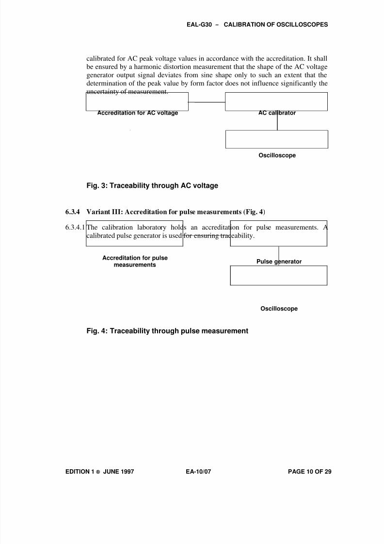
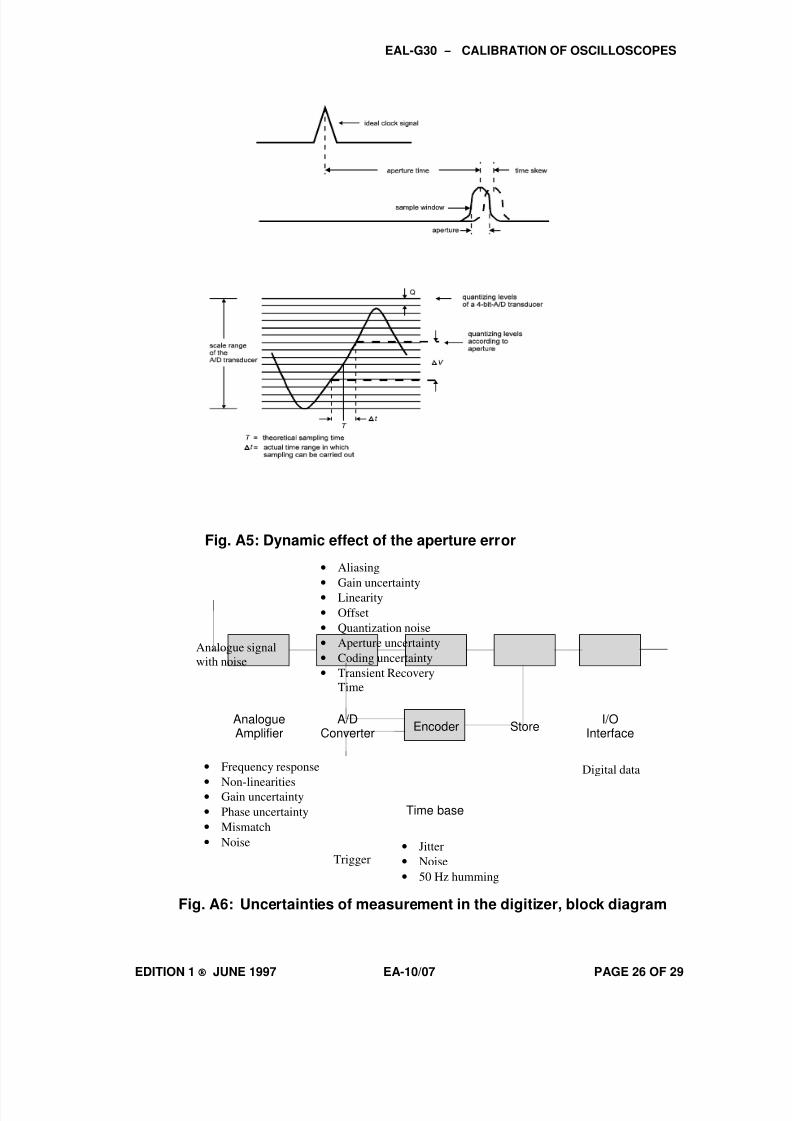
Fig. A5: Dynamic effect of the aperture error
Fig. A6: Uncertainties of measurement in the digitizer, block diagram
I/O
Interface
Digital data
Time base
Analogue
Amplifier
A/D
Converter Encoder Store
Analogue signal
with noise
• Aliasing
• Gain uncertainty
• Linearity
• Offset
• Quantization noise
• Aperture uncertainty
• Coding uncertainty
• Transient Recovery
Time
Trigger
• Frequency response
• Non-linearities
• Gain uncertainty
• Phase uncertainty
• Mismatch
• Noise • Jitter
• Noise
• 50 Hz humming

8/3/2019 Ea 10 07 Osciloscopios
http://slidepdf.com/reader/full/ea-10-07-osciloscopios 27/29
EAL-G30 - CALIBRATION OF OSCILLOSCOPES
EDITION 1 ® JUNE 1997 EA-10/07 PAGE 27 OF 29
A3.3.1 Linearity
(a) The deviation L from the linear shape shall be calculated from individual
measurements between the main graticule lines within the scope of the time
base measurement (Fig. A7).
L =−T T
T p p
p
i imax min ( ) Ln i
n
= −=
∑1
1
T T p pi
2
(A6)
T pi max maximum period
T pi min minimum period
T p averaged period
Fig. A7: Time base linearity check. Screen display in the completelybalanced state at ideal linearity

8/3/2019 Ea 10 07 Osciloscopios
http://slidepdf.com/reader/full/ea-10-07-osciloscopios 28/29
EAL-G30 - CALIBRATION OF OSCILLOSCOPES
EDITION 1 ® JUNE 1997 EA-10/07 PAGE 28 OF 29
A4 Calibration with HF voltage
(a) Up to 30 MHz, commercial AC voltage calibrators are available into which a
generator and a voltmeter are integrated to form one device. Because of theirgood long-term stability, thermal converters are suitable as HF voltage
standards. For frequencies up to 1 GHz, they are manufactured on a
commercial basis with a coaxial T junction integrated into the coaxial housing
(e.g. the Ballantine 1396A type). For commercial devices at frequencies up to
100 MHz (e.g. Fluke A55, Ballantine 1394A and 1395A), the junction shall be
attached externally. Thermal converters can be calibrated with measuring
uncertainties of ≤ 1 % by tracing them back to a national HF voltage standard
at frequencies up to 1 GHz.
(b) For accurate HF voltage and amplitude measurements, the position of the
reference plane shall be taken into account, for example, when adapters or
connecting lines are used. The reflection of voltage waves will lead to a voltage
standing wave along the line if the characteristic impedance of the line Z l
and
the terminating impedance Z E
connected to the line are not equal. The
magnitude of the voltage |U IN
| at the input differs from the magnitude U Eat
the output of a loss-free line of electrical length L. For a loss-free line,
|U IN
| = |cos(2π·L / wl ) + j·Z l / Z
E·sin(2π·L / wl )|·|U
E| (A7)
is valid, where wl is the wavelength of the HF signal. Likewise, the line
attenuation can lead to a difference between |U IN| and |U E|. Cable attenuationsare proportional to the root of the measuring frequency. Thin cables can show
attenuations of well over 1 dB/m at 1 GHz.
(c) Thermal converters are always, and power meters are predominantly,
instruments measuring rms values. For oscilloscopes, however, usually the
amplitude, i.e. the peak value, of the voltage is calibrated; therefore, as pure a
sinusoidal measurement signal as possible shall be ensured, i.e. the generator
shall be of sufficient spectral purity.
(d) The output and input impedances of commercial HF generators, oscilloscopes
for higher frequencies and HF power meters as well as the characteristicimpedance of the coaxial lines used are generally more or less well matched to
the nominal value of the reference characteristic impedance Z 0
of the HF line
system (in most cases 50 Ω). The deviation of an impedance Z X
from the
nominal value is characterized by the reflection coefficient
Γ = (Z X-Z 0)/(Z X+Z 0). (A8)
(d) When voltage measurements are made with a calibrated power meter and a T
junction (6.5.2.1) or with a calibrated generator (6.5.2.2), significant
uncertainties can arise if the input conductance of the power meter (GL) or

8/3/2019 Ea 10 07 Osciloscopios
http://slidepdf.com/reader/full/ea-10-07-osciloscopios 29/29
EAL-G30 - CALIBRATION OF OSCILLOSCOPES
oscilloscope (GOS) is not known exactly. The input conductance GIN of a
device can be determined if its input reflection coefficient Γ IN is known:
( )G G GIN O
IN
IN
OIN
IN IN cos= −
+= −
+ +11
11 2
2
2
2
2Γ Γ
Γ Γ Γ ϕ
(A9)
and GO = 1/ Z O. If only the modulus of Γ IN is known, the uncertainty of
measurement can be estimated when GO is used instead of GIN (GL in Eq.(3),
GOS in Eq.(5)). If Γ 2
<< Γ << 1, (A9) will reduce to
( )G GIN O IN cos≈ −1 2 Γ ϕ (A10)
(e) If the reflection coefficients of the generator (index G), of the power meter (N)
and of the oscilloscope (OS) are not negligible when the voltage Û is measuredat the oscilloscope using a generator and a calibrated power meter (6.5.2.2), Û is given by
( )[ ]Û P G b= 2 / OS (A11)
where
( )b = 1 OS
G OS
−−
−Γ
Γ Γ
Γ Γ
2
2
2
1
1
G N(A12)
and P is the power fed into the oscilloscope (traceable to the calibrated power meter).(f) If the phases of the reflection coefficient are not known and a correction is
therefore not possible, Eq. (A12) can be used to estimate the resulting
uncertainty of measurement of the voltage Û . If the generator and the
oscilloscope are to be connected by a line, the generator shall be calibrated
together with this line as a unit.
(g) As the uncertainties of the power measurement and of the conductance
measurement, which may be of the order of a few percent, contribute to the
overall uncertainty of the amplitude measurement, the relative uncertainty of
amplitude measurement may be of the order of several percent when this
method is used.


