
Introduction to Dynamic Linear Models
• Dynamic Linear Models (DLMs) or state space models
define a very general class of non-stationary time series
models.
• DLMs may include terms to model trends, seasonality,
covariates and autoregressive components.
• Other time series models like ARMA models are
particular DLMs.
• The main goals are short-term forecasting, intervention
analysis and monitoring.
• We will not focus as much on concepts like
autocorrelation or stationary process.
1

• A Normal DLM is defined with a pair of equations
Yt = F′
t θt + εt; (observation equation)
θt = Gtθt−1 + ωt; (evolution equation)
t = 1, 2, . . . , T
– Yt is the observation at time t. We assume this is to
be a scalar but could also be a vector.
– θt = (θt,1, . . . , θp,1)′
is the vector of parameters at time
t and of dimension p × 1.
– F′
t is the row vector (dimension 1 × p) of covariates at
time t
– Gt is a matrix of dimension p × p known as evolution
or transition matrix.
– Usually Ft and Gt are completely specified and
2
Ft = F , Gt = G.
– εt is the observation error at time t and ωt is the
evolution error (p × 1 vector).
– For a Normal DLM, εt ∼ N(0, Vt) and ωt ∼ N(0,Wt).
– εt is independent of εs, ωt is independent of ωs for
t 6= s. ε′s independent of ω′s.
• Mostly we will discuss the Bayesian analysis of these
models the counterpart being the Kalman Filter.
• The main reference on Bayesian DLMs, West, M. and
Harrison, J. (1997) Bayesian Forecasting and Dynamic
Models, 2nd ed. Springer Verlag, New York.
• In general Dynamic Models are given by two pdfs:
f(Yt|θt) and g(θt|θt−1)
3

which define a conditional dependence structure between
observations (Yt) and parameters (θt)
• DLMs have a sequential nature and from a Bayesian
approach, one of its main targets, is
p(θt|Dt) , t = 1, 2, . . . , T
the posterior distribution of θt given all the information
available at time t, i.e., Dt = {Y1, Y2, . . . , Yt}
• The simplest “dynamic model” is well known:
Yt = µ + εt, εt ∼ N(0, σ2)
• In DLM notation θt = µ, F′
t = 1, ωt = 0 and Gt = 1.
4

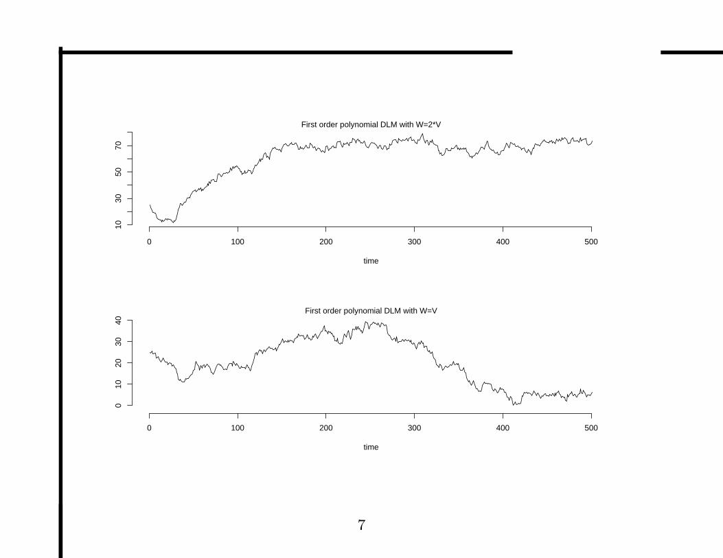
• A generalization is the First order polynomial DLM
Yt = µt + εt; εt ∼ N(0, Vt)
µt = µt−1 + ωt; ωt ∼ N(0,Wt)
• The evolution equation allows smooth changes of the
mean level. Wt is a scalar greater than zero.
• West and Harrison use νt instead of εt or νt ∼ N(0, Vt).
• Equivalently the first order polynomial DLM is written as
(Yt|µt) ∼ N(µt, Vt); (µt|µt−1) ∼ N(µt−1,Wt)
• Lets consider the constant case with Vt = V , Wt = W ,
V = 1, µ0 = 25. Plots show simulations for W = 2V ,
W = V , W = V/20 and W = V/2.
5

time
0 100 200 300 400 500
1620
2428
First order polynomial DLM with W=V/20
time
0 100 200 300 400 500
510
1520
25
First order polynomial DLM with W=V/2
6
time
0 100 200 300 400 500
1030
5070
First order polynomial DLM with W=2*V
time
0 100 200 300 400 500
010
2030
40
First order polynomial DLM with W=V
7

# Function to simulate 1st order polynomial DLM
genfoDLM=function(V,n,del)
{
yt=rep(NA,n+1)
W=V/del
mut=rep(NA,(n+1))
mut[1]=25
for(i in 2:(n+1))
{
mut[i]=mut[i-1]+rnorm(1,0,sqrt(W))
yt[i]=mut[i]+rnorm(1,0,sqrt(V))
}
return(mut,yt)
}
8

• Notice that for the first order polynomial DLM
E(Yt+k|µt) = E(µt+k|µt) = µt
E(Yt+k|Dt) = E(µt|Dt) ≡ mt
which is useful for short term forecasting.
Inference for the First order Polynomial DLM
• Suppose the sequences Vt and Wt are known for all time t.
• At time 0 the prior for µ0 is N(m0, C0) and denoted by
(µ0|D0) ∼ N(m0, C0).
• We want to find (µt|Dt), the posterior for µt given Dt
and we will proceed sequentially.
– We start from the posterior at time t − 1,
(µt−1|Dt−1) N(mt−1, Ct−1)
9

– From this posterior we can get the prior at time t,
(µt|Dt−1) N(mt−1, Ct−1) where Rt = Ct−1 + Wt.
– We can obtain the predictive at time t − 1,
(Yt|Dt−1) ∼ N(ft, Qt) where ft = mt−1 and
Qt = Rt + Vt.
– Using Bayes’ theorem we can get the posterior at time
t, (µt|Dt) ∼ N(mt, Ct) and the recursive equations:
mt = mt−1 + Atet;
Ct = AtVt
At = Rt/Qt
et = Yt − ft
• Proof (by induction)
10

• We start from the posterior at time t − 1;
(µt−1|Dt−1) ∼ N(mt−1, Ct−1).
• Using the evolution equation and Normal linear theory,
µt = µt−1 + ωt, we get (µt|Dt−1) ∼ N(mt−1, Ct−1 + Wt)
(initial at time t). Rt ≡ Ct−1 + Wt
• From the observation equation Yt = µt + εt,
E(Yt|µt,Dt−1) = µt and V ar(Yt|µt,Dt−1) = Rt + Vt ≡ Qt,
then (Yt|Dt−1) ∼ N(mt−1, Qt)
• By Bayes’ Theorem,
p(µt|Dt−1) ∝ f(yt|µt−1)p(µt|Dt−1)
• Then
p(µt|Dt−1) ∝ exp
{
− 1
2Vt
(Yt − µt)2
}
exp
{
− 1
2Qt
(µt − mt−1)2
}
11

• After some algebra and completing a square for µt
p(µt|Dt−1) ∝ exp
{
− Qt
2RtVt
(
µt −(
Rtyt + Vtmt−1
Qt
))2}
∝ exp
{
− 1
2AtVt
(
µt −(
Rt(yt − mt−1) + (Vt + Rt)mt−1
Qt
))2}
• et = Yt − ft is known as the one-step predictive forecast.
• Since At = Rt/(Rt + Vt) (adaptive coefficient), then
0 ≤ At ≤ 1.
• Given that mt = At(et) + mt−1 = AtYt + (1 − At)mt−1 as
At → 1, mt ≈ Yt. As At → 0, mt ≈ mt−1.
12

Forecasting k-steps ahead
• Determine the distribution (Yt+k|Dt). From the
observation equation we have that,
Yt+k = µt+k + εt+k
• From the evolution equation,
µt+k = µt+k−1 + ωt+k
= µt+k−2 + ωt+k−1 + ωt+k
...
= µt +k∑
j=1
ωt+j
13

• Then,
Yt+k = µt +k∑
j=1
ωt+j + εt+k
• Since the posterior for µt at time t is (µt|Dt) ∼ N(mt, Ct)
then (Yt+k|Dt) ∼ N(mt, Qt(k)) where
Qt(k) = Ct +k∑
j=1
Wt+j + Vt+k
• mt is the predictive mean and Qt(k) is the predictive
variance.
• Example (W&H pag. 40) Data is monthly sales of a
pharmaceutical company of a product “Kurit”.
Approximately 100 units are sold every month.
14

• It is expected that a new advertisement campaign leads
to increases in demand of this product.
• At t = 0, a 30% increase in sales is expected. A range of
80 units is equivalent to 4√
C0.
• Then C0 = 400 and the prior at time 0 is
(µ0|D0) ∼ N(130, 400).
• The proposed model is:
Yt = µt + εt; εt ∼ N(0, 100)
µt = µt−1 + ωt; ωt ∼ N(0, 5)
(µ0|D0) ∼ N(130, 400)
15

2 4 6 8
130
140
150
Kurit data and posterior means for mu_t
2 4 6 8
0.2
0.4
0.6
0.8
Adaptive coefficient
16

2 4 6 8
8010
012
014
016
018
0Kurit data with one−step forecast
17

Kurit example
t Qt ft At Yt et mt Ct
0 130.0 400
1 505 130.0 0.80 150 20.0 146.0 80
2 185 146.0 0.46 136 -10.0 141.4 46
4 139 141.9 0.28 154 12.1 145.3 28
6 130 142.6 0.23 148 5.3 143.9 23
9 126 142.2 0.21 146 3.9 143.0 20
10 125 143.0 0.20
18

• One of the main advantages of the Bayesian approach for
DLMs is the ease to incoporate external information.
• For the Kurit example, at t = 9, the posterior and
one-step forecast distributions are
(µ9|D9) ∼ N(143, 20)
(Y10|D9) ∼ N(143, 125)
• Suppose that a competitive product (BURNIT) is
withdrawn from the market.
• At t = 10, patients that were prescribed BURNIT will
switch to a competitor. This information is denoted as
S9.
• Our company estimates a 100 % increase in KURIT
19

demand which translates to E(µ10|D9, S9) = 286
• There is a large uncertainty about this figure which is
expressed as (ω10|D9, S9) = N(143, 900) leading to the
following revised distributions,
µ10 = µ9 + ω10; (µ10|D9, S9) ∼ N(286, 920)
Y10 = µ10 + ε10; (Y10|D9, S9) ∼ N(286, 1020)
• Then, A10 = 920/1020 increases from 0.2 to 0.9 providing
a faster adaptation to the inmediately forthcoming data.
• If Y10 = 326, then e10 = 326 − 286 = 40 and
(µ10|D10) ∼ N(322, 90) where mt = 286 + 0.9(40) = 322
and Ct = 0.9(100) = 90.
• For a first-order polynomial DLM with constant
20

variances Vt = V and Wt = W , as t → ∞, At → A and
Ct → C = AV where
A =r
2
(
√
1 +4
r− 1
)
; r =W
V
• The one-step ahead forecast function mt = E(Yt+1|Dt)
takes the limit form:
mt = (1 − A)mt−1 + AYt = mt−1 + Aet
• As part of the DLM recursive equations, we have that
Rt = Ct−1 + W so in the limit (t → ∞),
R = C + W
• Also, Rt = At(Rt + V ) or Rt(1 − At) = AtV and in the
21

limit this implies that R(1 − A) = AV or
R =AV
1 − A=
C
1 − A
• Combining both equations for R, we obtain that
W =AC
1 − A
and W is a fixed proportion of C.
• This is a natural way of thinking about the evolution
variance, the addition of the error term ωt leads to an
increase uncertainty of W = 100A/(1 − A)% of C.
• If δ = 1 − A, it follows that R = C/δ and
W = (1 − δ)C/δ.
• Since for the first order polynomial DLM, the limiting
22

behavior is rapidly acheived, we can adopt a discount
factor δ for all t by choosing
Wt = Ct−1(1 − δ)/δ
• This DLM is not constant but quickly converges to a
constant DLM with Vt = V and Wt = rV with
r = (1 − δ)2/δ since
C−1t = V −1 + R−1
t = V −1 + δC−1t−1
= V −1[1 + δ + δ2 + . . . + δt−1] + δtC−10
so the limiting case of Ct is C = (1 − δ)V .
23

Unknown observational variance
• In the case of a constant variance Vt = V that is
unknown and Wt = V W ∗
t , where W ∗
t is known , the
Bayesian analysis leads to specific equations for the
relevant posterior distributions.
• The DLM is given by
Yt = µt + εt; εt ∼ N(0, V )
µt = µt−1 + ωt; ωt ∼ N(0, V W ∗
t )
• The prior is specified as
– (µ0|D0, V ) ∼ N(m0, V C∗
0 )
– For φ = 1/V ; (φ|D0) ∼ G(n0/2, d0/2).
• The values m0, C∗
0 , n0 and d0 are treated as known.
24

• For t = 1, . . . , T we have the recursive equations,
R∗
t = C∗
t−1 + W ∗
t ;
ft = mt−1;
Q∗
t = R∗
t + 1
et = Yt − ft
At = R∗
t /Q∗
t
C∗
t = R∗
t − A2t Q
∗
t
mt = mt−1 + Atet
• and the following distributions,
(µt−1|Dt−1, V ) ∼ N(mt−1, V C∗
t−1); (posterior at time t − 1)
(µt|Dt−1, V ) ∼ N(mt−1, V R∗
t); (prior at time t)
(Yt|Dt−1, V ) ∼ N(ft, V Q∗
t); (one-step predictive)
25

(µt|Dt, V ) ∼ N(mt, V C∗
t); (posterior at time t)
• For the precision φ = V −1:
– (φ|Dt−1) ∼ Ga(nt−1/2, dt−1/2).
– (φ|Dt) ∼ Ga(nt/2, dt/2).
where nt = nt−1 + 1 and dt = dt−1 + ε2t /Qt.
• Proof At time t − 1,
p(φ|Dt−1) ∝ φnt−1
2−1exp
(
−dt−1
2φ
)
• Also,
f(Yt|Dt−1, φ) ∝ φ1/2exp(
−φ(Yt − mt−1)2/2Q∗
t
)
• By Bayes’ theorem, p(φ|Dt) ∝ f(Yt|Dt−1, φ)p(φ|Dt−1)
which leads to the Ga(nt/2, dt/2).
26

Exchange Rates Example
• USA/UK exchange rate data from January 1975 to July
1984.
• The data has short-term variation about a changing level.
• First order polynomial DLM was considered with
evolution variances given by discount factors
(δ = 0.7, 0, 8, 0.9 and 1.0).
• The prior distribution is defined by m0 = 0, C0 = 1,
n0 = 1 and d0 = 0.01.
• The degree of adaptation to data increases as δ decreases.
27

Exchange rate and lowess with f=0.2
Time
y
1976 1978 1980 1982
−6
−4
−2
02
46
28

**
* **
*
*
* *
*
*
**
*
*
*
* *
** *
* * *
*
*
*
*
*
*
*
*
*
*
*
*
*
* *
*
*
*
*
*
*
*
* *
*
*
*
*
* *
*
*
*
*
*
*
*
**
*
*
*
*
*
*
*
*
*
* **
*
*
*
*
* *
*
*
** *
*
*
***
* *
*
*
*
*
*
* *
*
*
*
0 20 40 60 80 100
−6
−4
−2
02
46
Estimated level of exchange rate
Index
0.70.80.91
Discount factor
29

• Each value of δ defines a different model.
• To compare between models, the 3 adopted criteria are:
– The mean absolute deviation, MAD =∑T
t=1 |et|.– The mean square error, MSE =
∑Tt=1 e2
t /115
– The third summary is the observed predictive density
for all the data
p(YT , YT−1, . . . , Y1|D0) =T∏
t=1
p(Yt|Dt−1)
• This third measure is a likelihood function for δ.
• LLR is the log-likelihood ratio of the predictive density
relative to the model δ = 0.1
30

Exchange Rates example
δ MAD√
MSE LLR
1.0 0.019 0.024 0.00
0.9 0.018 0.022 3.62
0.8 0.018 0.022 2.89
0.7 0.018 0.023 0.96
31

Code for first order DLM in file ’code9.s’
update.dlm=function (Y,delta, m.0, C.0, n.0, S.0) {
N <- length(y)
m =n=C=R=Q=S=f=A=e=rep( NA,N )
Y = c(NA,Y)
C[1] <- C.0
m[1] <- m.0
S[1] <- S.0
n[1] <- n.0
for (t in 2:N ) {
n[t] <- n[t-1] + 1
W[t] <- C[t-1] * (1-delta) / delta
R[t] <- C[t-1] + W[t]
f[t] <- m[t-1]
32

Q[t] <- R[t] + S[t-1]
A[t] <- R[t] / Q[t]
e[t] <- Y[t] - f[t]
S[t] <- S[t-1]+(S[t-1]/n[t] )*(e[t]^2/Q[t] - 1)
m[t] <- m[t-1] + A[t]*e[t]
C[t] <- A[t]*S[t]
}
return (list(m=m,C=C, R=R,f=f,Q=Q,n=n,S=S))
}
33


