
TAMPERE UNIVERSITY OF TECHNOLOGY
Department of Information Technology
Duane Petrovich
Sequential Monte Carlo Methodsfor Personal Positioning
Master of Science Thesis
Subject approved by the Department Council on 7.12.2005
Examiners: Prof. Ioan Tabus
Prof. Robert Piche
Lic.Tech. Kari Heine

Preface
This thesis was written while working in the Personal Positioning Algorithms
Research Group at Tampere University of Technology and was funded by Nokia
Corporation. I would like to express my gratitude to prof. Robert Piche for
keeping me employed and to prof. Ioan Tabus for participating in the examination
of this thesis. Sincere thanks goes to Lic.Tech. Kari Heine for patience with
all of my “quick” questions that went on for hours. Additional thanks goes to
M.Sc. Simo Ali-Loytty, M.Sc. Niilo Sirola, and Henri Pesonen.
Tampere, 22th May 2006
Duane Petrovich
ii

Contents
Abstract v
Symbols vi
Abbreviations and Acronyms xi
1 Introduction 1
1.1 Organization . . . . . . . . . . . . . . . . . . . . . . . . . . . . . 2
2 Bayesian Estimation 3
2.1 Historical Notes . . . . . . . . . . . . . . . . . . . . . . . . . . . . 4
2.2 Mathematical Background . . . . . . . . . . . . . . . . . . . . . . 5
2.3 Bayesian Inference . . . . . . . . . . . . . . . . . . . . . . . . . . 7
2.4 Probabilistic Models for Dynamic Systems . . . . . . . . . . . . . 8
2.5 Recursive Bayesian Filtering . . . . . . . . . . . . . . . . . . . . . 9
2.6 Bayesian Filtering Algorithms . . . . . . . . . . . . . . . . . . . . 10
2.6.1 Kalman Filter . . . . . . . . . . . . . . . . . . . . . . . . . 11
2.6.2 Extended Kalman Filter . . . . . . . . . . . . . . . . . . . 12
3 SMC Approximation of Bayesian Filter 14
3.1 Monte Carlo Background . . . . . . . . . . . . . . . . . . . . . . . 15
3.1.1 Classical Monte Carlo . . . . . . . . . . . . . . . . . . . . 15
3.1.2 Importance Sampling . . . . . . . . . . . . . . . . . . . . . 16
3.2 Particle Filtering . . . . . . . . . . . . . . . . . . . . . . . . . . . 19
3.2.1 Sequential Importance Sampling . . . . . . . . . . . . . . . 19
3.2.2 Sequential Importance Sampling/Resampling . . . . . . . . 23
3.2.3 Examples of Importance Distributions . . . . . . . . . . . 25
3.3 Auxiliary Particle Filters . . . . . . . . . . . . . . . . . . . . . . . 26
3.3.1 Empirical Mixtures and Auxiliary Variables . . . . . . . . 27
3.3.2 Examples of Importance Distributions for APF . . . . . . 31
3.4 Resampling . . . . . . . . . . . . . . . . . . . . . . . . . . . . . . 34
3.4.1 Algorithms . . . . . . . . . . . . . . . . . . . . . . . . . . 35
3.4.2 Resampling Schedule . . . . . . . . . . . . . . . . . . . . . 38
iii

iv
4 SMC for Personal Positioning 40
4.1 Literature Review of Related SMC Applications . . . . . . . . . . 41
4.2 Personal Positioning Background and Principles . . . . . . . . . . 41
4.2.1 Measurements . . . . . . . . . . . . . . . . . . . . . . . . . 42
4.2.2 Static Case . . . . . . . . . . . . . . . . . . . . . . . . . . 43
4.2.3 Dynamic Case . . . . . . . . . . . . . . . . . . . . . . . . . 44
4.3 Simulation Set 1: Testbench . . . . . . . . . . . . . . . . . . . . . 45
4.3.1 Description . . . . . . . . . . . . . . . . . . . . . . . . . . 45
4.3.2 Multiple Trajectories: EKF vs PF at Different Sample Sizes 47
4.3.3 Comparing PFs with Different Importance Distributions . 51
4.4 Simulation Set 2: Comparing PF Posterior Approximations . . . . 54
4.4.1 Comparing Distributions with χ2-tests . . . . . . . . . . . 54
4.4.2 Probability Binning . . . . . . . . . . . . . . . . . . . . . . 55
4.4.3 Application to Linear and Gaussian Filtering Scenarios . . 56
4.4.4 Application to General Filtering Scenarios . . . . . . . . . 63
5 Conclusions 69

Abstract
TAMPERE UNIVERSITY OF TECHNOLOGY
Department of Information Technology
Institute of Signal Processing
Petrovich, Duane: Sequential Monte Carlo Methods for Personal Positioning
Master of Science Thesis, 70 pages
Examiners: prof. Ioan Tabus, prof. Robert Piche, Lic.Tech. Kari Heine
Evaluated by the Department Council in June 2006
The location of a mobile device can be estimated using signals from satellite and
cellular network based systems. Positioning technologies have numerous appli-
cations and consequently, are an active area of research. Bayesian estimation is
an attractive approach, but the models of measurements typically encountered
in positioning result in an intractable solution. In addition, analytic approxima-
tions of the models, e.g. linearizations, can often be inadequate and lead to poor
results. An alternative approach is numerical approximation.
In this thesis, we present a survey of sequential Monte Carlo (SMC) methods and
illustrate their use in positioning. We include examples of well-known importance
distributions, along with a brief discussion of resampling techniques. For com-
pleteness, this thesis also provides a review of the basics of Bayesian estimation
and Monte Carlo based methods.
We have implemented and tested SMC methods in a number of simulations in-
tended to resemble positioning environments. The improvement of SMC over an
extended Kalman filter is most apparent when using only base station measure-
ments and is not significant when using only satellite measurements. With fewer
measurements, a larger sample size may be required for reliable estimates; for
this reason, incorporating as much information as possible, e.g. base station sec-
tor and maximum range, is advised. Using our motion and measurement models,
more computationally expensive importance distributions do not give significant
improvements. Finally, the use of a multivariate binning technique is considered
as a feasible alternative criterion to compare the performance of SMC.
v

Symbols
General
·T Transpose of a vector or matrix
·−1 Inverse of a matrix
\ Set difference
⊆ Improper subset
· · · Unordered set
(· · · ) Ordered set
b·c Floor function, i.e. rounding to nearest integer towards zero
‖·‖ Euclidean norm of a vector
0 Vector of 0’s
A,B,C, . . . Arbitrary sets
a, b, c, . . . Arbitrary elements of a set
ab:c The ordered set (ab, . . . , ac)
a := b a is equal to b by definition
a ∝ b a is proportional to b
a ∈ A, a /∈ A a is in set A, a is not in set A
A×B Cartesian product of the sets A and B
B(Rn) Borel algebra of subsets of Rn
f : A→ B Function that maps elements from set A to set B
N Set of all natural numbers including 0
P Power set
R Set of all real numbers
Rn Set of all n-dimensional real numbers
Rm×n The set of all m by n matrices of real numbers
vi

SYMBOLS vii
Probability Theory
(Ω,F ,P) Probability space
(Ω,F) Measurable space
χ2, χ2a Chi-squared distribution, chi-squared distribution with a de-
grees of freedom
E [x ] Expectation of random variable x
Ep [x ] Expectation of random variable x having density p
F Collection of events
µ,C Mean vector and covariance matrix
N (µ,C) Normal distribution with mean µ and covariance C
ν(µ,C) Normal density with mean µ and covariance C
nx, ny Dimension of x and y
Ω, ω Sample space, sample point
P(A) Probability of event A ∈ FPx Probability distribution of random variable x
Px|y Probability distribution of random variable x given y = y
px Probability density of random variable x
px|y Conditional probability density of random variable x given y
ψ Test statistic
U[a,b] Uniform distribution over interval [a, b]
x ∼ P Random variable x is distributed according to P
x ∼ P x is a realization of random variable x with distribution P
V [x ] Variance of random variable x
Vp [x ] Variance of random variable x having density p

SYMBOLS viii
Bayesian Estimation
f Signal model function, f : Rnx → R
nx
F Matrix defining the linear signal model function, F ∈ Rnx×nx
F Jacobian matrix of signal model function f
γ Power spectral density of signal noise
h Observation model function, h : Rnx → R
ny
H Matrix defining the linear observation model function,
H ∈ Rny×nx
H Jacobian matrix of observation model function h
K Kalman gain
πa:b|c Conditional distribution of the signal process xa:b given real-
ization of the observation process y1:c = y1:c
πb|c Marginal conditional distribution of the signal process xb
given realization of the observation process y1:c = y1:c
Σv,Σw Covariance matrix of a signal noise and observation noise pro-
cess
σ2 Variance (scalar) of observation noise
V Signal noise process
W Observation noise process
X Signal process
Y Observation process

SYMBOLS ix
Monte Carlo
βj The jth unnormalized first-stage weight
βj The jth normalized first-stage weight
δx Delta-Dirac unit mass located at x
N The number of samples
Neff Effective sample size
Neff Approximation of effective sample size
M The number of importance samples
µ, C The realized SMC estimate of mean µ and covariance C, re-
spectively
πNa:b|c The discrete weighted approximation of πa:b|c, based on N
samples
P, p Arbitrary target distribution and density, respectively
PN The discrete equally-weighted approximation of distribution
P , based on N samples
PN The discrete weighted approximation of distribution P , based
on N samples
pj The jth linearized model
P , p Empirical approximation of distribution P and density p, re-
spectively
Q, q Arbitrary importance distribution and density, respectively
Qj The jth distribution component of mixture importance distri-
bution
w(·) Unnormalized importance weight function
wi Normalized importance weight of xi
xi The ith importance sample of x
xi The ith unweighted sample of x

SYMBOLS x
Positioning
b, b Bias of pseudorange, delta pseudorange measurement
∆tk Time difference, tk − tk−1
rb Position of a base station
rs, us Position,velocity of a satellite
rsi
, usi
Position,velocity of the ith satellite
r,u User position, velocity
V (·) Loss Function

Abbreviations and Acronyms
AOA Angle of Arrival
APF Auxiliary Particle Filter
BS Base Station
CDF Cumulative Distribution Function
CEP Circular Error Probability
EKF Extended Kalman Filter
ENU East-North-Up
GPS Global Positioning System
IID Independent and Identically Distributed
IS Importance Sampling
MC Monte Carlo
MCMC Markov Chain Monte Carlo
MS Mobile Station
MVU Minimum Variance Unbiased (estimator)
PF Particle Filter
RMSE Root Mean Square Error
RSS Received Signal Strength
RTD Round Trip Delay
SIR Sampling Importance Resampling
SIS Sequential Importance Sampling
SISR Sequential Importance Sampling/Resampling
SMC Sequential Monte Carlo
SV Space Vehicle
TOA Time of Arrival
xi
Chapter 1
Introduction
The problem of determining one’s location from measurements is an age-old
problem that is still a relevant research topic today. Satellite-based systems,
e.g. Global Positioning System (GPS), can be effective in providing accurate
position estimates, but have difficulty in urban areas or indoors due to atten-
uated signals. Local wireless networks, e.g. cellular networks, offer positioning
capabilities, but typically with less accuracy than that of satellite-based systems.
Different systems have their strengths and weaknesses, and a given system is gen-
erally not suitable for all possible scenarios. Positioning methods that are able
to combine measurements from multiple sources, e.g. both satellite systems and
cellular networks, are therefore advantageous.
The Bayesian formulation of the positioning problem conveniently allows mea-
surements from different sources to be incorporated in the estimation of position
coordinates. This approach inherently involves treating uncertainty as probabil-
ity distributions. Theoretically, we have an optimal probability distribution that
describes everything we know about the position coordinates having received the
measurements. Unfortunately, the models of the measurements commonly used
in positioning result in an intractable optimal solution.
One approach is to use analytic approximations of the true models so that the
Bayesian solution becomes tractable. However, this can perform quite poorly if
the approximations are inadequate. Another approach is to solve the original, in-
tractable problem by numerical approximation. Monte Carlo based methods, also
known as sampling based methods, are computational methods that approximate
distributions with empirically simulated samples. Gelfand and Smith [1990] have
bluntly stated that “. . . the attraction of the sampling-based methods is their
computational simplicity and ease of implementation for users with computing
resources but without numerical analytic expertise.”
1

CHAPTER 1. INTRODUCTION 2
Sequential Monte Carlo methods, also known as particle filters, are a class of
techniques to approximate the optimal probability distribution recursively over
time. A practical Monte Carlo algorithm for filtering was introduced about a
decade ago and since then, the methods been the focus a great deal of research. In
this work, we review some of the theory behind sequential Monte Carlo methods
and illustrate their use in positioning.
1.1 Organization
This work is organized as follows. Bayesian estimation is discussed in Chapter 2.
We first introduce the ideas for the stationary case, and then extend the discussion
to dynamic systems. We describe two Bayesian algorithms, one optimal and one
suboptimal, that will be used later in the examples and simulations. Throughout
this work, we have avoided discussion of the construction of the model and have
focused on the estimation task given the models.
Sequential Monte Carlo is introduced in Chapter 3 and we present the methods in
two separate formulations. The choice of importance distribution is emphasized
as a design parameter and we give a number of examples. We conclude this
chapter with a brief introduction to some resampling techniques.
Having covered the basics of Bayesian estimation and the sequential Monte Carlo
approximation of the Bayesian filter, we apply the concepts to the positioning
problem in Chapter 4. We present empirical results illustrating filter performance
in different positioning environments and also comparing different importance
distributions. In addition, we apply a multivariate binning technique to the
comparison of sequential Monte Carlo methods. We give some concluding remarks
in Chapter 5.

Chapter 2
Bayesian Estimation
Our topic of interest is estimating the state of a system from noisy observations.
Kay [1993] identifies two approaches to estimation: classical and Bayesian. In
classical estimation, the state is assumed to be a deterministic but unknown
constant. One is then typically interested in the estimator that is unbiased with
minimum variance—the MVU estimator. On the other hand, Bayesian estimation
assumes the unknown state is a random variable with a particular realization
that we are to estimate. It earns the name Bayesian because the implementation
is based on Bayes’ theorem. One motivation for the Bayesian approach is the
convenient use of prior knowledge, which is not straightforward to incorporate
into classical estimation. Another motivation is that in situations when the MVU
estimator cannot be found, the Bayesian approach provides a framework to find
an estimator that performs well on the average [Kay 1993, pg. 309].
In this work, we will focus exclusively on Bayesian estimation. We start in Sec-
tion 2.2 by briefly covering the necessary mathematical concepts and notation. In
Section 2.3, we give a general introduction of the Bayesian framework describing
the basic principles for a static system. We work our way towards applying this
methodology to dynamic systems by first, introducing the needed probabilistic
models in Section 2.4 and then presenting the Bayesian recursion for dynamic
systems in Section 2.5. Finally, in Section 2.6, we present some well-known algo-
rithms for implementing the Bayesian solution in practice.
3

CHAPTER 2. BAYESIAN ESTIMATION 4
2.1 Historical Notes
The origins of modern estimation theory are usually traced back to the invention
of least squares. Around 200 years ago, Legendre and Gauss independently in-
vented and applied the method to determining the orbits of celestial bodies. In
Legendre’s approach, there was no probabilistic interpretation and the proposal
was just a convenient method that minimized a function of errors. It is gener-
ally accepted that Gauss and Laplace are responsible for the development of the
theory and a probabilistic interpretation. [Stigler 1981], [Merriman 1877]
During the late 1930s and early 40s, Kolmogorov and Wiener independently pro-
posed theory for the linear prediction of processes with statistical properties that
do not change in time, i.e. stationary processes. Wiener also worked on filtering
problems and, using frequency domain techniques, was able to formulate the op-
timum linear estimate of a stationary process corrupted by additive noise. It was
not until 1960, motivated by the coming space age and by the inadequacy of the
Wiener filter to deal with nonstationary problems, that the linear, nonstationary
filtering problem was solved by Kalman. [Haykin 1991], [Jazwinski 1970]
The history of nonlinear filtering is not as successful and is still a field of active
research. During the 60s and into the 70s, nonlinear filters relying on analyti-
cal approximations began to appear—most notably, the extended Kalman filter
and Gaussian sum filter, e.g. Alspach and Sorenson [1972]. In the early 1980s,
Benes published the optimal solution for a special class of nonlinear filtering
problems—a type of saturating process, see e.g. Farina et al. [2002]. This was
later generalized by Daum but there still is no optimal solution for all nonlinear
problems. [Daum 2005], [Anderson and Moore 1979]
Today, the state of the art in nonlinear filters includes a number of computational
methods, e.g. Monte Carlo based methods and numerical solutions for partial
differential equations, as well as new variations of the Kalman filter, e.g. the
unscented Kalman filter [Daum 2005].

CHAPTER 2. BAYESIAN ESTIMATION 5
2.2 Mathematical Background
In this work, an underlying probability space (Ω,F ,P) is assumed, where the
sample space Ω defines all possible outcomes, the σ-algebra F on Ω is the col-
lection of events of interest, and the probability measure P on the measurable
space (Ω,F) assigns a probability to each of these events. Let B(Rn) denote the
collection of Borel sets of Rn.
Definition 2.1. Let x be a random variable defined on some probability space
(Ω,F ,P) such that x : Ω → Rnx. The induced probability measure Px is referred
to as the probability distribution of x and is defined as
Px(A) := P(x ∈ A), A ∈ B(Rnx),
where we use the common shorthand notation
P(x ∈ A) := P (ω ∈ Ω | x(ω) ∈ A) .
Similarly, the conditional probability distribution Px|y of the random vari-
able x given the event y = y is defined such that
Px|y(A) := P (x ∈ A | y = y) , A ∈ B(Rnx).
Regarding notation, random variables will be denoted in bold font, i.e. x, while
realizations of random variables will be in plain font, i.e. x, and there is no explicit
notation for vectors. Note that both of the probability measures of Definition 2.1
are deterministic. We will avoid discussion of the random measures generated by
conditioning on a σ-algebra, see e.g. Crisan [2001], as it is outside the scope of
this work.
In this work, a probability density px of a distribution Px and a conditional
probability density px|y(·|y) of a conditional distribution Px|y are assumed to
exist without explicit notation and satisfy the following
Px(A) =
∫
A
px(x) dx
Px|y(A) =
∫
A
px|y(x|y) dx,
where again A ∈ B(Rnx). Subscripts on the density may be omitted if the random
variable in question is obvious, e.g. p(x|y) instead of px|y(x|y).
The Lebesgue integral, see e.g. Gariepy and Ziemer [1995, pg. 133-134], provides
a generalization of the Riemman integral that will be useful for our purposes. Ex-
pectation of some function f of a random variable is defined using the (Lebesgue)
integral with respect to a probability measure P , i.e.
E [ f(x) ] :=
∫f(x)P (dx), (2.1)
CHAPTER 2. BAYESIAN ESTIMATION 6
where the function f is assumed to be P -integrable.
The usefulness of the Lebesgue integral in (2.1) can be illustrated as follows. If the
probability measure P has a density p (with respect to the Lebesgue measure),
then (2.1) is taken to be
E [ f(x) ] =
∫f(x) p(x) dx.
If the probability measure P is a discrete function taking values pi at the points
xi for i = 1, . . . N , then (2.1) is taken to be
E [ f(x) ] =N∑
i=1
f(xi) pi.
In this work, Lebesgue integration is used so that expectations of continuous and
discrete random variables are under the same framework.
Maybeck [1979, pg. 78-80] derives various forms of a conditional probability den-
sity, alternatively known as Bayes’ rule. The result is derived as a limit because
conditioning on an event with zero probability, e.g. y = y when y is continuous,
can be problematic.
Definition 2.2. Various forms of Bayes’ rule for (continuous or discrete) ran-
dom variables are given by
p(x|y) =p(x, y)
p(y)=p(y|x) p(x)
p(y),
where p(y) is a nonzero normalization constant given by
p(y) =
∫p(x, y) dx =
∫p(y|x) p(x) dx.
We will often need to discuss a time-sequence of random variables, and so we take
the following definition from Maybeck [1979, pg. 133].
Definition 2.3. Let Ω be a sample space and T ⊆ R. Then a stochastic or
random process X is a real function defined on the product space Ω × T such
that for any t ∈ T , X(·, t) =: xt is a random variable.
The stochastic process may also be denoted by X = (xt)t∈T . If T is discrete,
as it will always be in this work, then we can refer to the stochastic process as
a stochastic sequence and explicitly denote this by using a time index k. A
process that we will encounter quite frequently is the Markov process.

CHAPTER 2. BAYESIAN ESTIMATION 7
Definition 2.4. A stochastic process X = (xk)k∈N is a Markov process (of
order one) if for all k ∈ N\0,
p(xk|x0, x1, . . . , xk−1) = p(xk|xk−1).
Such Markov processes are completely defined by the initial distribution Px0and
the conditional distributions Pxk|xk−1, also called transition kernels [Robert and
Casella 1999, pg. 141].
We do not explicitly define the distribution of a finite stochastic sequence because
it can be considered as the distribution of a random variable, i.e. a stacked vector
of all the individual random variables in time.
2.3 Bayesian Inference
We often have a quantity that we are interested in estimating and want to make
some sort of inference on this quantity based on observed data. Bayesian infer-
ence refers to the use of probability statements to combine prior knowledge with
the information gained from observing data. This inherently involves treating
uncertainty and belief as probability distributions—a fundamental characteristic
of the Bayesian philosophy.
Let us denote our quantity of interest x and the observed data y, which are con-
sidered to be realizations of the random variables x and y respectively. The term
“hidden” is often used when referring to x to emphasize that we infer information
only through measurements, i.e. x itself is unobserved. We start with a priori
knowledge of our quantity of interest. This represents what we know about x
before any data is received and is given in terms of a probability distribution
with density p(x). Next, we need a model that relates the observed data to the
hidden quantity. The observations are assumed to be from some distribution that
depends on our quantity; if the observations were independent of our quantity
then there would be no inference possible. Let p(y|x) denote both the condi-
tional density of the observations and the likelihood function, depending on the
argument1.
Using Bayes’ rule for random variables, we have
p(x|y) ∝ p(y|x) p(x). (2.2)
1Note that py|x(y|x) is a function of both x and y. If we fix x and treat py|x as a function
of y, it is a density. But, if we fix y and treat py|x as a function of x, then it is called the
likelihood function and does not necessarily have the properties of a density, e.g. integrating to
unity [Lee 1997, pg. 34].

CHAPTER 2. BAYESIAN ESTIMATION 8
The conditional distribution having conditional density p(x|y) represents our a
posteriori knowledge in that it embodies all available statistical information
and is the complete solution to the problem based on the initial assumptions [Lee
1997]. We will use the term prior to refer to both the distribution and density
of the a priori knowledge, and similarly use the term posterior to refer to both
the distribution and density of the a posteriori knowledge.
We should emphasize that, in practice, the motivating factor for a Bayesian ap-
proach is typically the various estimates that can be obtained from the posterior,
i.e. not the posterior distribution itself. In Bayesian estimation, we use the
posterior distribution to form estimates, e.g. by taking expectations with respect
to the posterior distribution or by maximizing the posterior density. It is for
these reasons that we are interested in determining the posterior distribution.
2.4 Probabilistic Models for Dynamic Systems
Consider now a time-sequence of values we are interested in estimating (xk)∞k=0
and a corresponding time-sequence of measurements (yk)∞k=1. Recall that in
Bayesian estimation, the unknown value we want to estimate, as well as the
observations, are considered to be realizations of random variables. To apply the
Bayesian framework to this estimation, we must define these random variables
in terms of probabilistic models. This section formulates the time-sequence esti-
mation task in such a framework so that we can proceed to present the Bayesian
solution.
We define two stochastic processes X = (xk)∞k=0 and Y = (yk)
∞k=1, where
xk ∈ Rnx and yk ∈ R
ny . The process X is called the unobserved (hidden) signal
process and is modelled as a (first-order) Markov process defined by an initial
distribution Px0and transition kernel Pxk|xk−1
, i.e.
x0 ∼ Px0, xk | x0:k−1, y1:k−1 ∼ Pxk|xk−1
. (2.3)
The process Y is called the observation process and is modelled as
yk | x0:k, y1:k−1 ∼ Pyk|xk. (2.4)
We will refer to (2.3) as the signal model, as it describes how the signal evolves
with time, and (2.4) as the observation model, as it defines how the observa-
tions are related to the signal.

CHAPTER 2. BAYESIAN ESTIMATION 9
2.5 Recursive Bayesian Filtering
We will often use the term filtering to refer to a specific type of estimation
task when discussing time-sequence processing; in particular, to distinguish it
from smoothing and prediction. Recall that we have a time-sequence of values
we are interested in estimating (xk)∞k=0 and a corresponding time-sequence of
measurements (yk)∞k=1. In this context, filtering refers to the estimation of xk
using all the information received up to time k, i.e. y1, y2, ..., yk. In smoothing,
we use measurements received after k and in prediction, we use only measurements
available before k. [Anderson and Moore 1979, pg. 10-11]
Using the Bayesian framework, we will form the probability distribution of the
signal process conditioned on the realization of the observation process. Let the
conditional distribution of the signal be denoted as
πa:b|c := Pxa:b|y1:c. (2.5)
At any time k, the density of the joint posterior distribution π0:k|k is given
by Bayes’ rule as
p(x0:k|y1:k) =p(y1:k|x0:k) p(x0:k)
p(y1:k),
where the denominator is a normalizing constant independent of x0:k given by
p(y1:k) =
∫p(y1:k|x0:k) p(x0:k) dx0:k
:=
∫∫. . .
∫p(y1:k|x0:k) p(x0:k) dx0 dx1 . . . dxk.
However, it is more useful in practice to have the density of the marginal or
filtering distribution πk|k and form a recursion that obtains this solution from
the previous solution πk−1|k−1 in two stages: prediction and update.
Suppose at time k − 1, the density for the posterior πk−1|k−1 is available; this
embodies everything we know about xk−1, i.e. the state of the signal at time
k − 1, having received all the measurements y1, . . . , yk−1. The prediction stage
consists of applying the signal model (2.3) to this density to describe what we
know about xk, i.e. the state of the signal at time k, before receiving any data
from time k. The prediction distribution πk|k−1 embodies this information
and has a density given via [Jazwinski 1970, pg. 174]
p(xk|y1:k−1) =
∫p(xk, xk−1|y1:k−1) dxk−1
=
∫p(xk|xk−1, y1:k−1) p(xk−1|y1:k−1) dxk−1
=
∫p(xk|xk−1) p(xk−1|y1:k−1) dxk−1. (2.6)

CHAPTER 2. BAYESIAN ESTIMATION 10
The Markov assumption of the signal was used in the third equality. Equation
(2.6) is often referred to as the Chapman-Kolmogorov equation.
When the measurement at time k becomes available, the update stage then
uses Bayes’ rule with the measurement model (2.4) to obtain the density of the
posterior πk|k given by [Jazwinski 1970, pg. 174]
p(xk|y1:k) =p(yk|xk) p(xk|y1:k−1)
p(yk|y1:k−1),
where the denominator is a normalizing constant independent of xk given by
p(yk|y1:k−1) =
∫p(yk|xk) p(xk|y1:k−1) dxk.
Common estimates used in Bayesian filtering include the conditional mean and
covariance, which are expectations with respect to the probability measure πk|k
and are given respectively by
µk = E [xk | y1:k ]
=
∫xk p(xk|y1:k) dxk (2.7)
Ck = E[(xk − µk)(xk − µk)
T | y1:k
]
=
∫(xk − µk)(xk − µk)
T p(xk|y1:k) dxk. (2.8)
2.6 Bayesian Filtering Algorithms
We shift from our general discussion of the models in probabilistic terms to in-
troduce an example stochastic system. These system equations will aid in
presenting the algorithms. Let
xk = fk−1(xk−1) + vk−1 (2.9)
yk = hk(xk) +wk, (2.10)
where V = (vk)∞k=0 and W = (wk)
∞k=1 are the signal noise and observation
noise processes, respectively. The subscript on the functions fk−1 and hk indi-
cates a possible dependence on time. To emphasize the relation of the system
equations to the probabilistic models of Section 2.4, we can write the following
p(xk|xk−1) = pvk−1(xk − fk−1(xk−1) )
p(yk|xk) = pwk( yk − hk(xk) ),
where pvk−1is the density of vk−1 and pwk
is the density of wk.

CHAPTER 2. BAYESIAN ESTIMATION 11
By imposing certain restrictions on the models, the number of parameters needed
by a filter to characterize the exact posterior distribution can be finite. Such
cases are rare but are of interest because we can derive algorithms to compute
the optimal solution. Optimal algorithms include the Kalman filter for linear-
Gaussian cases, grid-based methods when the state-space is discrete and finite,
and the Benes and Daum filters for a special class of nonlinear filtering problems
[Ristic et al. 2004]. The Kalman filter is described in Section 2.6.1.
In general, however, there is no finite set of parameters to describe the posterior.
Approximations are then typically introduced. Suboptimal algorithms include
the extended Kalman filter, approximate grid-based methods, Gaussian sums,
and particle filters [Ristic et al. 2004]. The extended Kalman filter is described
in Section 2.6.2 and the remainder of this work is devoted to particle filters.
2.6.1 Kalman Filter
Suppose the posterior distribution at a given time k−1 is Gaussian and therefore,
is completely characterized by a mean vector µk−1 and covariance matrix Ck−1.
By restricting the filtering problem to be linear and Gaussian, then both the
prediction distribution πk|k−1 and posterior distribution πk|k of the next time
step will be also be Gaussian [Ristic et al. 2004, pg. 7-8]. A linear filtering
problem is one in which the functions fk−1 and hk of the system equations are
linear functions of the state of the signal, while a Gaussian filtering problem is
one in which the noise processes V and W in the system equations are Gaussian
distributed. We will further assume that the noise processes are zero-mean and
independent in time and of each other. For filtering problems that are linear and
Gaussian, the system equations can be written as
xk = Fk−1xk−1 + vk−1
yk = Hkxk +wk,
where vk−1 ∼ N (0,Σvk−1), wk ∼ N (0,Σwk
), and Fk−1 and Hk are matrices,
possibly time-dependent.
The Kalman filter algorithm [Kalman 1960] recursively computes the parameters
of the Gaussian prediction and posterior distributions of the signal. It is assumed
that we know the matrices Fk and Hk and the noise covariances Σvk−1and Σwk
,
have received the observation yk, and have the previous solution (µk−1, Ck−1). In
this case,
πk|k−1 = N (µ−k , C
−k ), πk|k = N (µk, Ck),

CHAPTER 2. BAYESIAN ESTIMATION 12
where [Ristic et al. 2004, pg. 8]
µ−k = Fk−1µk−1 (2.11a)
C−k = Σvk−1
+ Fk−1Ck−1FTk−1 (2.11b)
µk = µ−k +Kk
(yk −Hkµ
−k
)(2.11c)
Ck = C−k −KkHkC
−k (2.11d)
Kk = C−k H
Tk
[HkC
−k H
Tk + Σwk
]−1. (2.11e)
2.6.2 Extended Kalman Filter
When the functions fk−1 and hk of the system equations are nonlinear functions of
the state of the signal, then this is a nonlinear filtering problem and the previ-
ous algorithm is no longer applicable. In this case, one approach is to approximate
the functions by a truncated Taylor expansion evaluated at the current estimate
of the signal. This method is known as the extended Kalman filter (EKF) and
will be briefly described here.
The nonlinear functions can be approximated as
fk−1(xk−1) ≈ fk−1(µk−1) + Fk−1(xk−1 − µk−1)
hk(xk) ≈ hk(µ−k ) + Hk(xk − µ−
k ),
where Fk−1 denotes the Jacobian of fk−1(xk−1) evaluated at µk−1 and Hk de-
notes the Jacobian of hk(xk) evaluated at µ−k . Higher order terms of the Taylor
expansion can be included at additional computational cost. Substituting these
approximations of the nonlinear functions into the system equations (2.9) and
(2.10), then we have new system equations given by
xk = Fk−1xk−1 + vk−1 + (fk−1(µk−1) − Fk−1µk−1)
yk = Hkxk +wk + (hk(µ−k ) − Hkµ
−k ).
The Kalman filter from Section 2.6.1 can now be applied to this approximate
model as it is now linear and still assumed Gaussian. The algorithm equations of
(2.11) are now [Ristic et al. 2004, pg. 20]
µ−k = fk−1(µk−1) (2.12a)
C−k = Σvk−1
+ Fk−1Ck−1FTk−1 (2.12b)
µk = µ−k +Kk
(yk − hk(µ
−k )
)(2.12c)
Ck = C−k −KkHkC
−k (2.12d)
Kk = C−k H
Tk
[HkC
−k H
Tk + Σwk
]−1
. (2.12e)

CHAPTER 2. BAYESIAN ESTIMATION 13
There are, in fact, a number of variations of the EKF although we have presented
only the most basic algorithm here, see e.g. Daum [2005] for a brief overview. It
is important to keep in mind that these EKF methods are approximations and
have no optimality properties [Kay 1993, pg. 451].
Chapter 3
Sequential Monte Carlo
Approximation of Bayesian Filter
Sequential Monte Carlo (SMC) methods, also known as particle filters (PFs),
implement the recursive Bayesian filter with Monte Carlo (MC) simulation. The
posterior distribution is approximated by a simulated set of samples with appro-
priate weights. Rather than solving an approximate problem exactly, as with the
EKF, SMC methods solve an exact problem by numerical approximation. This
is most attractive in nonlinear and non-Gaussian situations where the integrals
of (2.6) and (2.7) are not tractable.
There are different formulations of the SMC methods and in this work, we have
taken the approach to present two separate formulations. The first is the probably
the most common perspective, which is sequential importance sampling followed
by a resampling step, see e.g. Liu and Chen [1998]; Doucet et al. [2000]; Ris-
tic et al. [2004]. The second approach is the mixture formulation of Pitt and
Shephard [1999], also known as the auxiliary particle filter. Some authors have
described the first formulation from within this mixture framework, see e.g. Car-
penter et al. [1999], but we keep them separate here to facilitate comparing this
work to the majority of existing literature. We conclude this chapter with a brief
discussion of resampling techniques.
In Liu et al. [2001], it is mentioned that the sequential importance sampling
method dates back to the 50s with applications in statistical physics. Doucet
[1998] notes that there was work during the 1960s and 70s in automatic control
that used SMC methods. It is the work of Gordon et al. [1993] that is generally
credited for demonstrating the use of resampling in the SMC context, which, in
turn, began the recent surge of interest in SMC methods.
14

CHAPTER 3. SMC APPROXIMATION OF BAYESIAN FILTER 15
3.1 Monte Carlo Background
This section introduces two MC-based methods, classical Monte Carlo and im-
portance sampling. The MC methods we will be concerned with approximate
a distribution by a finite collection of realizations of random variables, called
samples or particles. The following definition will be needed.
Definition 3.1. The delta-Dirac unit mass located at x is a function denoted
by δx such that
δx(A) =
1 if x ∈ A
0 if x /∈ A,
where A ∈ B(Rnx) if x ∈ Rnx and A ∈ P (x1, . . . , xN) if x ∈ x1, . . . , xN, with
P denoting the power set.
The process of obtaining realizations of a random variable x with a given dis-
tribution will be called simulating from the distribution or according to the
distribution. It has also been described in the literature as generating or draw-
ing samples. In general, it is not always feasible to simulate samples according to
a given distribution. See e.g. Devroye [1986] for discussions on random number
generation.
3.1.1 Classical Monte Carlo
Let xiNi=1 be a realization of xiN
i=1, which is a set of independent and iden-
tically distributed (IID) random variables with some distribution P . Then an
unweighted discrete approximation of P is given by
P ≈ PN :=1
N
N∑
i=1
δxi .
Integrals of the form
I =
∫f(x) p(x) dx, (3.1)
for some P -integrable function f , can be approximated by the classical Monte
Carlo approximation
I ≈
∫f(x)PN(dx) =
1
N
N∑
i=1
f(xi). (3.2)
The justification for the approximation in (3.2) relies on the strong law of large
numbers, see e.g. Shiryayev [1984, pg. 366]. This then implies that the empirical
distribution PN approximates the true distribution P . Note that the use of the
Lebesgue integral in (3.2) is important for our formulation of the approximations.

CHAPTER 3. SMC APPROXIMATION OF BAYESIAN FILTER 16
3.1.2 Importance Sampling
An alternative method of approximating P relies on the use of importance
sampling (IS). The idea relies on writing (3.1) as∫f(x) p(x) dx =
∫f(x)
p(x)
q(x)q(x) dx,
where q is a density of probability distribution Q. Notice that the left-hand side
is an expectation with respect to the probability measure P , i.e. Ep [ f(x) ], and
the right-hand side is an expectation with respect to the probability measure
Q, i.e. Eq [ f(x) p(x)/q(x) ]. If xiNi=1 is a realization of a set of IID random
variables with distribution Q, then provided that the support of q includes the
support of p, approximations of integrals of the form in (3.1) can be given by the
importance sampling approximation
I ≈
∫f(x)
p(x)
q(x)QN(dx) =
1
N
N∑
i=1
f(xi)p(xi)
q(xi). (3.3)
The justification for this approximation is for the same reasons as the classical
Monte Carlo approximation. Importance sampling is often introduced as a solu-
tion to the scenario when one cannot sample directly from P but can sample from
a “close” distribution Q, known as the importance or proposal distribution,
and evaluate the ratio p(x)/q(x).
If the densities p and q are only known up to proportionality, then we can use
a similar, but different approximation of (3.1). Assume that we can evaluate
w(x) ∝ p(x)/q(x), called the unnormalized importance weight. If xiNi=1 is
a realization of a set of IID random variables with distribution Q, then
I =
∫f(x)w(x) q(x) dx∫w(x) q(x) dx
≈1N
∑Ni=1 f(xi)w(xi)
1N
∑Ni=1 w(xi)
, (3.4)
again, provided that the support of q includes the support of p. Note that the
same random samples are used in the numerator and denominator for the ap-
proximation in (3.4).
For our purposes, it will be convenient to formulate the approximation of (3.4)
in terms of a probability measure that approximates P . A weighted discrete
approximation of P is given by
P ≈ PN :=N∑
i=1
wi δxi , (3.5)
where
w(xi) ∝ p(xi)/q(xi), wi :=w(xi)
∑Nj=1w(xj)
. (3.6)

CHAPTER 3. SMC APPROXIMATION OF BAYESIAN FILTER 17
The approximation of (3.4) can be equivalently written as
I ≈
∫f(x) PN(dx) =
N∑
i=1
wi f(xi). (3.7)
The wi terms are the normalized importance weights, and the division by the
sum of weights in (3.6) will be referred to as normalization. Note that we may
omit the “normalized” or “unnormalized” term when discussing the importance
weights if it is clear from notation which we are referring to.
In this work, we will only consider importance sampling for scenarios where p and
q are known up to proportionality. The requirement mentioned concerning the
support of the importance density q including the support of the true density p
will be assumed and not explicitly repeated for the rest of this work. Alternative
methods for approximating a distribution that cannot be sampled from directly
include rejection sampling and Markov Chain Monte Carlo (MCMC),
see e.g. Robert and Casella [1999]. These methods will not be discussed in this
work.
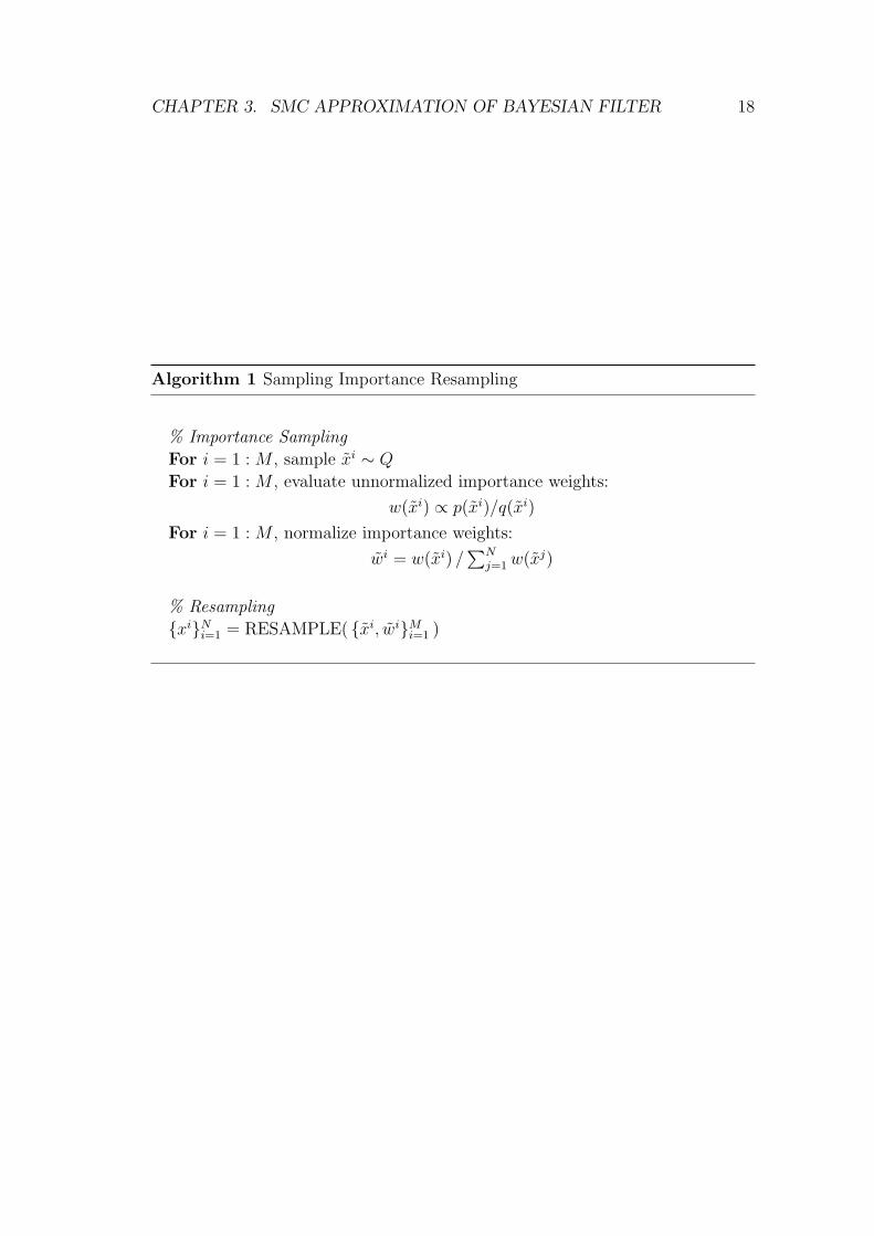
Sampling Importance Resampling (SIR)
An algorithm for generating equally-weighted samples approximately distributed
according to a distribution P using an importance distribution Q is known as
sampling importance resampling (SIR) [Rubin 1987]. It consists of first
drawing M proposal points from the importance distribution and calculating the
importance weights. The points and weights define a weighted discrete approxi-
mation, see (3.5), from which we can sample N points from. The effectiveness of
the SIR algorithm depends on M being sufficiently large which, in turn, depends
on how close P and Q are. As M/N → ∞, the N samples will be IID from P
[Rubin 1987].
Sampling from a discrete distribution will be referred to as resampling. There
are various methods for resampling and we have devoted Section 3.4 to describing
these techniques. For now, we will refer to this resampling step in our algorithms
with a generic function “RESAMPLE”, which takes a set of samples and weights
as input, i.e. a weighted discrete distribution, and returns the resampled points
and, optionally, the new weights of the resampled points. The SIR algorithm is
given in Algorithm 1.
CHAPTER 3. SMC APPROXIMATION OF BAYESIAN FILTER 18
Algorithm 1 Sampling Importance Resampling
% Importance Sampling
For i = 1 : M , sample xi ∼ Q
For i = 1 : M , evaluate unnormalized importance weights:
w(xi) ∝ p(xi)/q(xi)
For i = 1 : M , normalize importance weights:
wi = w(xi) /∑N
j=1w(xj)
% Resampling
xiNi=1 = RESAMPLE( xi, wiM
i=1 )

CHAPTER 3. SMC APPROXIMATION OF BAYESIAN FILTER 19
3.2 Particle Filtering
Returning now to the filtering scenario, we aim to construct an approximation
to the joint posterior distribution π0:k|k and the marginal distribution πk|k. We
now apply IS to Bayesian filtering. The general idea is still to sample from some
importance distribution and compute importance weights, which forms a weighted
discrete approximation of a probability distribution. The difference here is that
we are now sampling realizations from a stochastic process and the probability
distribution that we are interested in approximating is the Bayesian posterior
distribution.
3.2.1 Sequential Importance Sampling
In this section, we describe the application of IS to the Bayesian filtering context.
We will also be interested in formulating this as a recursive algorithm. The re-
cursive formulation is important for online applications, where storage capacity
may be limited and fast estimates are required. However, Daum [2005] has sug-
gested that with the cheap, fast memory and powerful processors available today,
these reasons for preferring a recursive algorithm are often not an issue for many
applications.
Bayesian Filtering via IS
Recall the shorthand notation π0:k|k for the joint posterior distribution that was
defined as
πa:b|c := Pxa:b|y1:c.
Since, in general, it is not feasible to sample from π0:k|k, we adopt an IS approach.
Let Qx0:k|y1:kbe a different distribution that is “close” to π0:k|k that we can sample
from, i.e. an importance distribution, and let xi0:k
Ni=1 be a realization of a set of
IID random trajectories with distribution Qx0:k|y1:k. If we can evaluate the den-
sities p(x0:k|y1:k) and q(x0:k|y1:k) up to proportionality, then we have a weighted
discrete approximation to the joint posterior similar to (3.5) given by
π0:k|k ≈ πN0:k|k :=
N∑
i=1
wik δxi
0:k, (3.8)
where the importance weights are computed similar to (3.6) as
w(xi0:k) ∝
p(xi0:k|y1:k)
q(xi0:k|y1:k)
, wi =w(xi
0:k)∑Nj=1w(xj
0:k). (3.9)

CHAPTER 3. SMC APPROXIMATION OF BAYESIAN FILTER 20
This method, however, is not recursive. If we computed an IS approximation for
the distribution at time k− 1, then there is no mechanism to use this solution to
compute an IS approximation for the distribution at time k.
Bayesian Filtering via SIS
We aim to be able to compute an approximation of π0:k|k recursively, i.e. from our
approximation of π0:k−1|k−1. To do this, we must derive a recursive importance
weight update.
We write the density of the importance distribution as
q(x0:k|y1:k) = q(xk|x0:k−1, y1:k) q(x0:k−1|y1:k−1). (3.10)
The idea is that, having samples that are realizations from Qx0:k−1|y1:k−1, we can
obtain samples from Qx0:k|y1:kjust by augmenting each existing xi
0:k−1 with a
sample xik ∼ Qxk|x
i0:k−1
,y1:k, i.e. xi
0:k = (xi0:k−1, x
ik).
The importance weight update can be computed recursively as follows. From the
factorization of the posterior density given by
p(x0:k|y1:k) =p(yk, x0:k|y1:k−1)
p(yk|y1:k−1)(3.11)
∝ p(yk|x0:k, y1:k−1) p(x0:k|y1:k−1)
= p(yk|x0:k, y1:k−1) p(xk|x0:k−1, y1:k−1) p(x0:k−1|y1:k−1)
and the factorization of the importance density in (3.10), the normalized impor-
tance weights satisfy the following
wik ∝
p(xi0:k|y1:k)
q(xi0:k|y1:k)
∝p(yk|x
i0:k, y1:k−1) p(x
ik|x
i0:k−1, y1:k−1)
q(xik|x
i0:k−1, y1:k)
p(xi0:k−1|y1:k−1)
q(xi0:k−1|y1:k−1)
∝p(yk|x
i0:k, y1:k−1) p(x
ik|x
i0:k−1, y1:k−1)
q(xik|x
i0:k−1, y1:k)
wik−1. (3.12)
The p(yk|y1:k−1) term in (3.11) is a constant that often cannot be expressed in
closed-form. However, it is independent of i and can be left out of the weight
update since we need to evaluate the weights only up to proportionality.
The form of (3.12) is very general. We will restrict our attention to importance
distributions of the form
q(xk|x0:k−1, y1:k) = q(xk|xk−1, yk)

CHAPTER 3. SMC APPROXIMATION OF BAYESIAN FILTER 21
and models of the form in Section 2.4. Imposing these restrictions, the weight
update simplifies to
wik ∝
p(yk|xik) p(x
ik|x
ik−1)
q(xik|x
ik−1, yk)
wik−1. (3.13)
Having sampled from an importance distribution and computed the importance
weights, the weighted discrete approximation to the joint posterior can be formed
exactly as in (3.8). The difference here is that the sampling and weight update are
done recursively over time, hence the name sequential importance sampling
(SIS).
Notice that we can work with the marginal distribution πk|k rather than the joint
posterior π0:k|k. In practice, this means that instead of storing the full trajectory
of each particle, only the particles from the previous time step need to be stored
due to our Markov assumption of the signal. We should keep in mind that when
drawing samples of xk, we are, in fact, drawing samples of x0:k and just discarding
x0:k−1.
The SIS algorithm is given in Algorithm 2. Note that we have simplified the
initialization for the algorithm and assumed that we can sample from Px0.

CHAPTER 3. SMC APPROXIMATION OF BAYESIAN FILTER 22
Algorithm 2 Sequential Importance Sampling
% Initialize, k = 0
For i = 1 : N , sample xi0 ∼ Px0
For i = 1 : N , set wi0 = 1/N
For k = 1, 2, . . .
For i = 1 : N , sample xik ∼ Qxk|x
ik−1
,yk
For i = 1 : N , evaluate unnormalized importance weights:
w(xi0:k) ∝
p(yk|xik) p(x
ik|x
ik−1)
q(xik|x
ik−1, yk)
wik−1
For i = 1 : N , normalize importance weights:
wik = w(xi
0:k) /∑N
j=1w(xj0:k)

CHAPTER 3. SMC APPROXIMATION OF BAYESIAN FILTER 23
3.2.2 Sequential Importance Sampling/Resampling
Unfortunately, the SIS algorithm presented so far often performs quite poorly in
practice. It can happen that after only a few iterations of the algorithm, all but
one of the normalized importance weights are close to zero. This results in a large
computation effort being devoted to updating trajectories with little contribution
to the final estimate. Consequently, the algorithm will fail to adequately represent
the posterior distribution. Such a scenario has been described as a degeneracy
of the algorithm. [Doucet et al. 2000, pg. 199].
In Gordon et al. [1993], a resampling step is introduced so that at every time
step, N samples are drawn from the distribution of N weighted samples. This
effectively duplicates trajectories with large weight and removes particles with
negligible weight. This approach is generally considered to be what established
SMC as a practical filtering method. Roughly speaking, the resampling step
“rejuvenates” the sampler in the hope that it will improve results for future
states, although it does not improve the results for the current state [Liu and
Chen 1998, pg. 9]. This implies that any estimates formed from the sample set
should be computed before resampling.
We now give a general algorithm for the SIS/Resampling (SISR) filter in
Algorithm 3. Note that when resampling, this algorithm is just the SIR algorithm
with M = N to fit the filtering context.
Having a recursive algorithm that approximates the posterior distribution, we can
turn our attention to the estimates. Since expectations with respect to a weighted
discrete probability measure are conveniently evaluated using summations, see
(3.7), approximations of the conditional mean (2.7) and conditional covariance
(2.8) are given respectively by
µk ≈ µk :=N∑
i=1
wik x
ik
Ck ≈ Ck :=N∑
i=1
wik (xi
k − µk)(xik − µk)
T .

CHAPTER 3. SMC APPROXIMATION OF BAYESIAN FILTER 24
Algorithm 3 Sequential Importance Sampling/Resampling
% Initialize, k = 0
For i = 1 : N , sample xi0 ∼ Px0
For i = 1 : N , set wi0 = 1/N
For k = 1, 2, . . .
% Importance Sampling
For i = 1 : N , sample xik ∼ Qxk|x
ik−1
,yk
For i = 1 : N , evaluate unnormalized importance weights:
w(xi0:k) ∝
p(yk|xik) p(x
ik|x
ik−1)
q(xik|x
ik−1, yk)
wik−1
For i = 1 : N , normalize importance weights:
wik = w(xi
0:k) /∑N
j=1w(xj0:k)
% Resampling
[ xik, w
ik
Ni=1 ] = RESAMPLE( xi
k, wik
Ni=1 )

CHAPTER 3. SMC APPROXIMATION OF BAYESIAN FILTER 25
3.2.3 Examples of Importance Distributions
When approximating some probability distribution P using importance sampling,
the choice of importance distribution Q is arbitrary provided that the support
of q includes the support of p. However, some choices will perform better than
others and some choices will require more computational complexity than others.
In this section, we review a few well-known choices as examples.
Example 1: Prior Importance Distribution
Probably the most common choice of importance distribution is to use the prior,
i.e.
Qxk|xik−1
,yk= Pxk|x
ik−1
.
The normalized importance weights are given from (3.13) as
wik ∝
p(yk|xik) p(x
ik|x
ik−1)
q(xik|x
ik−1, yk)
wik−1
=p(yk|x
ik) p(x
ik|x
ik−1)
p(xik|x
ik−1)
wik−1
= p(yk|xik) w
ik−1.
This choice of importance distribution simplifies the algorithm: all that is needed
is to be able to simulate samples from Pxk|xik−1
and to evaluate the likelihood
p(yk|xik). However, exploring the state space without using the present mea-
surement yk, i.e. having the importance distribution independent of yk, can be
inefficient if the prior is not “close” to the posterior. It should be noted that this
was the choice of importance distribution in the seminal paper by Gordon et al.
[1993].
Example 2: Extended Kalman Importance Distribution
Another intuitive choice for the importance distribution results from linearizing
the model locally as with the EKF, see e.g. van der Merwe et al. [2000] and Ristic
et al. [2004]. In this case, each particle has an importance distribution that is a
Gaussian distribution with mean and covariance given by the EKF posterior. We
can then write the ith particle’s importance distribution as
Qxk|xik−1
,yk= N (µi
k, Cik)
CHAPTER 3. SMC APPROXIMATION OF BAYESIAN FILTER 26
where the EKF update is given from (2.12) as
µ−(i)k = fk−1(x
ik−1) (3.14a)
C−(i)k = Σvk−1
+ F ik−1C
ik−1F
Tk−1 (3.14b)
µik = µ
−(i)k +K i
k
(yk − hk(µ
−(i)k )
)(3.14c)
C ik = C
−(i)k −K i
k Hik C
−(i)k (3.14d)
Kik = C
−(i)k (H i
k)T
[H i
kC−(i)k (H i
k)T + Σwk
]−1
. (3.14e)
This means that if there are N particles, then the algorithm involves N extended
Kalman filter updates. Notice that this requires that the error covariance matrix
for each particle, i.e. C ik, be saved and propagated at every time step, as well as
resampled when resampling is performed.
The normalized importance weights are given from (3.13) as
wik ∝
p(yk|xik) p(x
ik|x
ik−1)
q(xik|x
ik−1, yk)
wik−1
=p(yk|x
ik) p(x
ik|x
ik−1)
ν(xik;µ
ik, C
ik)
wik−1,
where ν( · ;µ,C) is the density of a Gaussian distribution with mean µ and
covariance C.
The improvement from using this choice of importance distribution will depend
on whether the extended Kalman posterior is significantly different from the prior
and whether the inaccuracies introduced by the linearization are significant. The
computational aspect of performing a large number of EKF updates can also be
an issue. In fact, other Kalman related filters could be used in place of the basic
EKF that we have described. For example, the unscented Kalman filter was used
in the proposed particle filter of van der Merwe et al. [2000].
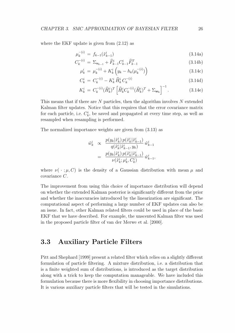
3.3 Auxiliary Particle Filters
Pitt and Shephard [1999] present a related filter which relies on a slightly different
formulation of particle filtering. A mixture distribution, i.e. a distribution that
is a finite weighted sum of distributions, is introduced as the target distribution
along with a trick to keep the computation manageable. We have included this
formulation because there is more flexibility in choosing importance distributions.
It is various auxiliary particle filters that will be tested in the simulations.

CHAPTER 3. SMC APPROXIMATION OF BAYESIAN FILTER 27
3.3.1 Empirical Mixtures and Auxiliary Variables
In the SISR framework previously presented, at each time step, we have N dif-
ferent prediction and posterior distributions—one for each particle. In this al-
ternative framework, at each time step, we approximate the true prediction and
posterior each by a single N component mixture. The empirical prediction
distribution and density are given respectively by
Pxk|y1:k−1=
N∑
j=1
wjk−1 Pxk|x
j
k−1
(3.15)
p(xk|y1:k−1) =N∑
j=1
wjk−1 p(xk|x
jk−1) (3.16)
and the empirical filtering distribution and density are given respectively
by
Pxk|y1:k(A) ∝
N∑
j=1
wjk−1
∫
A
p(yk|xk) p(xk|xjk−1) dxk (3.17)
p(xk|y1:k) ∝ p(yk|xk) p(xk|y1:k−1), (3.18)
where A ∈ B(Rnx).
Consider what happens when attempting importance sampling using these mix-
ture approximations. In the general case, evaluating the importance weight for
each sample will require evaluating N densities because the prior is a mixture
with N components, i.e.
w(xk) ∝p(xk|y1:k)
q(xk|y1:k)∝p(yk|xk)
∑Nj=1 w
jk−1 p(xk|x
jk−1)
q(xk|y1:k). (3.19)
As an example, drawing M samples would require M × N evaluations. This is
considered to be too computationally expensive to be a feasible algorithm sinceM
and N are typically large. Note that this problem does not arise when sampling
from the empirical prediction distribution, i.e. q(xk|y1:k) =∑N
j=1 wjk−1 p(xk|x
jk−1),
as the evaluations of the empirical prior density will cancel out of (3.19).
Pitt and Shephard [1999] propose to perform the filtering in a higher dimension.
By introducing a discrete auxiliary variable j, which refers to the index of a
mixture component, the mixture is essentially broken up over this new dimension,
see Figure 3.1. The joint density, i.e. the density of the joint distribution of state
and auxiliary variable, is defined as [Pitt and Shephard 1999, pg. 592]
p(xk, j|y1:k) ∝ wjk p(yk|xk) p(xk|x
jk−1) for j = 1, . . . N.
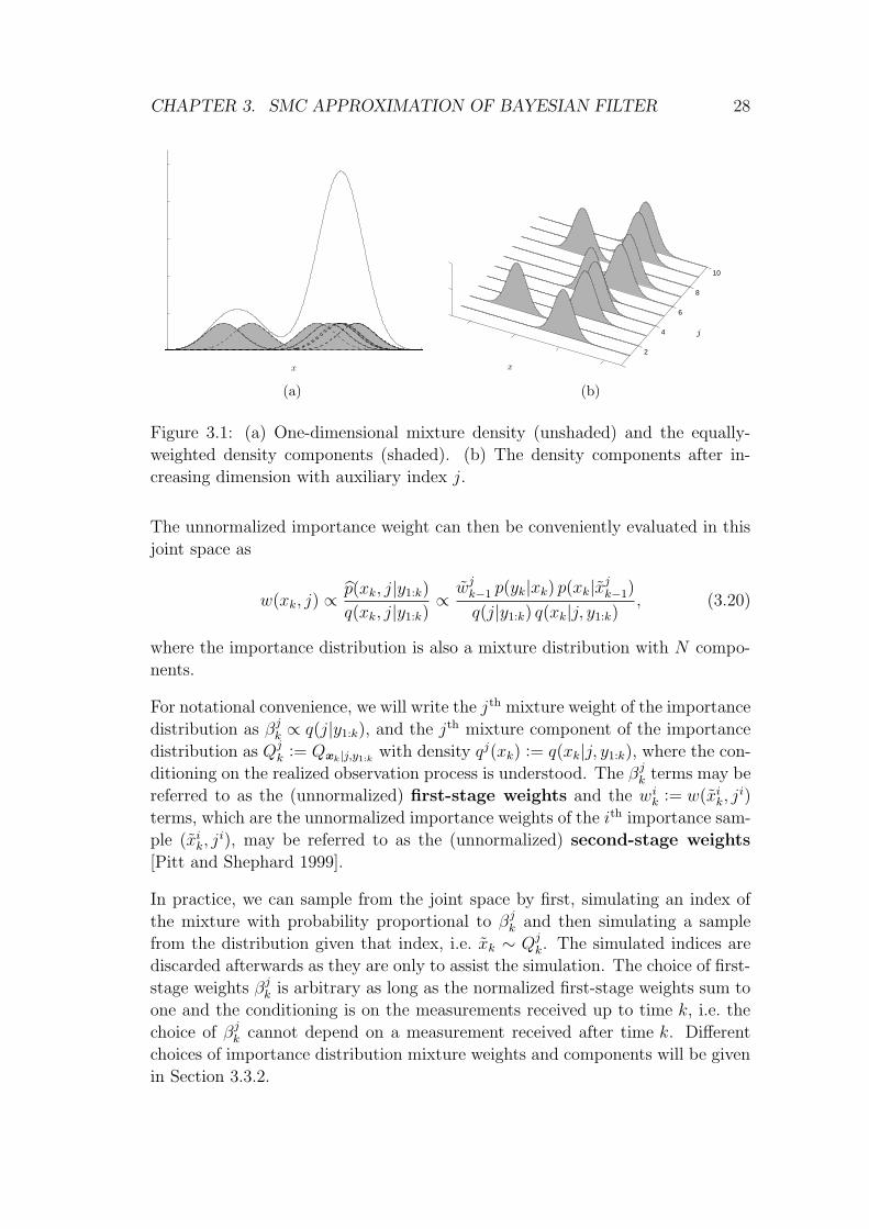
CHAPTER 3. SMC APPROXIMATION OF BAYESIAN FILTER 28
PSfrag replacements
x
(a)
2
4
6
8
10
PSfrag replacements
x
j
(b)
Figure 3.1: (a) One-dimensional mixture density (unshaded) and the equally-
weighted density components (shaded). (b) The density components after in-
creasing dimension with auxiliary index j.
The unnormalized importance weight can then be conveniently evaluated in this
joint space as
w(xk, j) ∝p(xk, j|y1:k)
q(xk, j|y1:k)∝wj
k−1 p(yk|xk) p(xk|xjk−1)
q(j|y1:k) q(xk|j, y1:k), (3.20)
where the importance distribution is also a mixture distribution with N compo-
nents.
For notational convenience, we will write the jth mixture weight of the importance
distribution as βjk ∝ q(j|y1:k), and the jth mixture component of the importance
distribution as Qjk := Qxk|j,y1:k
with density qj(xk) := q(xk|j, y1:k), where the con-
ditioning on the realized observation process is understood. The βjk terms may be
referred to as the (unnormalized) first-stage weights and the wik := w(xi
k, ji)
terms, which are the unnormalized importance weights of the ith importance sam-
ple (xik, j
i), may be referred to as the (unnormalized) second-stage weights
[Pitt and Shephard 1999].
In practice, we can sample from the joint space by first, simulating an index of
the mixture with probability proportional to βjk and then simulating a sample
from the distribution given that index, i.e. xk ∼ Qjk. The simulated indices are
discarded afterwards as they are only to assist the simulation. The choice of first-
stage weights βjk is arbitrary as long as the normalized first-stage weights sum to
one and the conditioning is on the measurements received up to time k, i.e. the
choice of βjk cannot depend on a measurement received after time k. Different
choices of importance distribution mixture weights and components will be given
in Section 3.3.2.

CHAPTER 3. SMC APPROXIMATION OF BAYESIAN FILTER 29
We now present an algorithm for the auxiliary particle filter (APF) in Algo-
rithm 4. Notice that the indices are simulated from a weighted discrete distribu-
tion, and so we have used our generic function “RESAMPLE” in the algorithm
to emphasize this. It has been suggested to sample M = N from the importance
distribution and skip the second “extra” resampling step altogether, see e.g. Car-
penter et al. [1999] and Ristic et al. [2004, pg. 50-51]. We will use this special
case frequently in the simulations.
It should be pointed out that even in the situation where we can sample from the
empirical filtering distribution (3.17), this will not produce IID samples from the
true posterior due to the finite mixture approximation [Pitt and Shephard 1999,
pg. 593]. We will refer to this point later.

CHAPTER 3. SMC APPROXIMATION OF BAYESIAN FILTER 30
Algorithm 4 Auxiliary Particle Filter
% Initialize, k = 0
For i = 1 : N , sample xi0 ∼ Px0
For i = 1 : N , set wi0 = 1/N
For k = 1, 2, . . .
% First-stage weights
For i = 1 : N , assign unnormalized 1st stage weights βik
For i = 1 : N , normalize 1st stage weights:
βik = βi
k /∑N
l=1 βlk
% Importance Sampling
Sample indices jiMi=1 = RESAMPLE( i, βi
kNi=1 )
For i = 1 : M , sample xik ∼ Qji
k
For i = 1 : M , evaluate unnormalized 2nd stage weights:
wik ∝
p(xik, j
i|y1:k)q(xi
k, ji|y1:k)
For i = 1 : M , normalize 2nd stage weights:
wik = wi
k /∑N
l=1wlk
% Resampling
[ xik, w
ik
Ni=1 ] = RESAMPLE( xi
k, wik
Mi=1 )

CHAPTER 3. SMC APPROXIMATION OF BAYESIAN FILTER 31
3.3.2 Examples of Importance Distributions for APF
We will now present four examples that illustrate the choice of mixture weights
βjk and components Qj
k for the importance distribution. We then derive the form
for the importance weights w(xk, j) by simply substituting our choice of βjk and
qj(xk) into (3.20). The second-stage weights wik can be evaluated by substituting
the importance sample (xik, j
i) into the function w(xk, j).
Example 1 is the basic example that samples from the empirical prior. Example
2 shows a different choice of weights, while Example 3 shows a different choice
of components. Example 4 illustrates an example using different weights and
components. These four examples will be used in the simulations and we have
used the naming convention of SIR1, SIR2, SIR3, and SIR4 so that we can easily
refer to them.
Example 1: Prior Components with Previous Weights (SIR1)
The common first example is to sample from the empirical prediction distribution,
i.e. Qxk|y1:k=
∑Nj=1 w
jk−1 Pxk|x
j
k−1
. From this form of the importance distribution,
we see that the first-stage weights are proportional to the second-stage weights
of the last time step, i.e. βjk ∝ wj
k−1, and the mixture components are equal to
the conditional prediction distributions, i.e. Qjk = P
xk|xj
k−1
. Notice that neither
the weights or the components in this choice of importance distribution use the
latest measurement.
We can derive the importance weights as
w(xk, j) ∝wj
k−1 p(yk|xk) p(xk|xjk−1)
βjk q
j(xk)
∝wj
k−1 p(yk|xk) p(xk|xjk−1)
wjk−1 p(xk|x
jk−1)
= p(yk|xk).
This means that the ith importance sample (xik, j
i) will be assigned the second-
stage weight wik ∝ p(yk|x
ik). For the remaining examples, we only give the form
of the importance weight function w(xk, j) and do not explicitly write the second-
stage weight wik to keep notation simple.

CHAPTER 3. SMC APPROXIMATION OF BAYESIAN FILTER 32
Example 2: Prior Components with Alternative Weights (SIR2)
Consider the following example to illustrate a convenient choice of first-stage
weights1. Pitt and Shephard [1999] propose using an importance distribution
that treats the likelihood p(yk|xk) of the jth mixture component as the constant
p(yk|ξjk), where ξj
k is the mean, the mode, a draw, or some other likely value
associated with the density of xk | xjk−1. The empirical filtering distribution
(3.17) is approximated using the importance distribution
Qxk|y1:k(A) ∝
N∑
j=1
wjk−1 p(yk|ξ
jk)
∫
A
p(xk|xjk−1) dxk
=N∑
j=1
wjk−1 p(yk|ξ
jk)Pxk|x
j
k−1
(A) A ∈ B(Rnx).
This means that our importance mixture consists of the mixture components
given by the transition distributions Qjk = P
xk|xj
k−1
again, but now with the first-
stage weights βjk ∝ wj
k−1 p(yk|ξjk). The intention is that we will simulate more
samples from those transition distributions that are associated with large likeli-
hood and hopefully, this will lead to a more accurate particle representation of
the target distribution.
The importance weights can be derived as
w(xk, j) ∝wj
k−1 p(yk|xk) p(xk|xjk−1)
βjk q
j(xk)
∝wj
k−1 p(yk|xk) p(xk|xjk−1)
wjk−1 p(yk|ξ
jk) p(xk|x
jk−1)
=p(yk|xk)
p(yk|ξjk).
In our simulations, SIR2 will always use the mean of the density of xk | xjk−1 for
ξjk.
Example 3: Kalman Components with Previous Weights (SIR3)
Using the prior distributions for the mixture components of the importance dis-
tribution, i.e. Qjk = P
xk|xj
k−1
, is often a convenient choice because it can be com-
putationally cheap to simulate samples from them and the second-stage weights
1This example has been described in the literature as the auxiliary particle filter, see e.g. Ris-
tic et al. [2004, pg. 49-52], whereas we present it as an example of an auxiliary particle filter,
see Pitt and Shephard [1999].

CHAPTER 3. SMC APPROXIMATION OF BAYESIAN FILTER 33
that follow are relatively easy to compute. However, other mixture components
can be used to design better approximations of the empirical filtering distribution.
The posterior distributions of the Kalman filter can also be used as mixture
components. For nonlinear filtering scenarios, a local linearization of the models,
as in the EKF, can be used. This means that Qjk = N (µj
k, Cjk), where
µ−(j)k = fk−1(x
jk−1) (3.21a)
C−(j)k = Σvk−1
(3.21b)
µjk = µ
−(j)k +Kj
k
(yk − hk(µ
−(j)k )
)(3.21c)
Cjk = C
−(j)k −Kj
k Hjk C
−(j)k (3.21d)
Kjk = C
−(j)k (Hj
k)T
[Hj
kC−(j)k (Hj
k)T + Σwk
]−1
(3.21e)
and Hjk is the Jacobian matrix of hk evaluated at fk−1(x
jk−1). Comparing this
with the extended Kalman importance distribution in the SISR framework, note
that here there is no error covariance propagated from the previous time step,
i.e. compare (3.21b) with (3.14b).
If we choose Qxk|y1:k=
∑Nj=1 w
jk−1 N (µj
k, Cjk), we have an importance distribu-
tion defined by the mixture weights βjk ∝ wj
k−1 and the mixture components
Qjk = N (µj
k, Cjk). The importance weights are then given by
w(xk, j) ∝wj
k−1 p(yk|xk) p(xk|xjk−1)
βjk q
j(xk)
∝wj
k−1 p(yk|xk) p(xk|xjk−1)
wjk−1 ν(xk;µ
jk, C
jk)
=p(yk|xk) p(xk|x
jk−1)
ν(xk;µjk, C
jk)
.
Example 4: Kalman Components with Alternative Weights (SIR4)
Note that while Example 2 introduced a convenient choice for alternative mixture
weights, the choice of mixture components did not use the latest measurement.
Example 3, on the other hand, introduced a convenient choice for the mixture
components, while the mixture weights did not use the latest measurement. In
Heine [2005], an example is given that uses both these design parameters. The
Kalman posteriors are again used for the mixture components of the importance
distribution, but now with alternative weights.
The EKF uses approximations of the true models so that the approximate models
are linear and Gaussian. We write the jth component’s linearized model as pj and

CHAPTER 3. SMC APPROXIMATION OF BAYESIAN FILTER 34
substitute these approximations into the empirical filtering distribution (3.17) to
derive an importance distribution. Define the constants cjk as
cjk :=
∫
Rnx
pj(yk|xk) pj(xk|x
jk−1) dxk.
Then we have an importance distribution as
Qxk|y1:k(A) ∝
N∑
j=1
wjk−1
∫
A
pj(yk|xk) pj(xk|x
jk−1) dxk
=N∑
j=1
wjk−1 c
jk
∫Apj(yk|xk) p
j(xk|xjk−1) dxk∫
Rnxpj(yk|xk) pj(xk|x
jk−1) dxk
=N∑
j=1
wjk−1 c
jk N (A;µj
k, Cjk), A ∈ B(Rnx),
where µjk and Cj
k again are the jth extended Kalman posterior mean and covari-
ance given by (3.21). In this case, the constants cjk have a closed-form solution
given by [Heine 2005]
cjk = ν(yk; hk
(fk−1(x
jk−1)
), Hj
k Σvk−1(Hj
k)T + Σwk
).
The importance distribution is defined by the first-stage weights, which are
βjk ∝ wj
k−1 cjk, and the distribution components, which are the extended Kalman
posteriors Qjk = N (µj
k, Cjk). The importance weights are then given by
w(xk, j) ∝wj
k−1 p(yk|xk) p(xk|xjk−1)
βjk q
j(xk)
∝wj
k−1 p(yk|xk) p(xk|xjk−1)
wjk−1 c
jk ν(xk;µ
jk, C
jk)
=p(yk|xk) p(xk|x
jk−1)
cjk ν(xk;µjk, C
jk)
.
3.4 Resampling
The two main design choices in SMC are the choice of the importance distribution
and the type of resampling. Various importance distributions were given in the
examples of Section 3.2.3 and Section 3.3.2, so we now turn our attention to the
resampling step.
One way of thinking about the resampling step is that the objective is to approx-
imate the weighted discrete approximation PM with an equally-weighted discrete

CHAPTER 3. SMC APPROXIMATION OF BAYESIAN FILTER 35
approximation PN . Often, M and N are chosen to be equal, but we keep the
notation separate. The resampling algorithms we will focus on will generate a
set of equally-weighted samples xiNi=1 from the weighted discrete distribution
defined by xi, wiMi=1. Various methods for resampling will be briefly reviewed
in Section 3.4.1.
Although referred to in Section 3.2.2 as the key to successfully applying MC
methods to the sequential context, resampling does introduce other problems.
The resampling step introduces repeated points into the sample set, which can
lead to a lack of particle “diversity”. This has been referred to as sample impov-
erishment [Ristic et al. 2004, pg. 43]. For this reason, different ideas have been
proposed concerning the resampling schedule, i.e. performing the resampling
step only on some chosen time steps. This will be discussed in Section 3.4.2.
3.4.1 Algorithms
This section will discuss several different algorithms and heuristics that have been
suggested for resampling in the particle filter. These methods are introduced with
the use of the cumulative distribution function (CDF). We write the CDF
of the indices of the discrete distribution as
Fw(j) :=
j∑
i=1
wi, for j = 1, . . . ,M
and the inverse CDF as
F−1w (u) := j, for qj−1 < u ≤ qj,
where qj =∑j
i=1 wi and q0 = 0.
Multinomial Resampling
Consider the simulation of an IID sample from a weighted discrete distribution,
i.e. the realization of xiNi=1 where xi ∼ PM =
∑Mj=1 w
j δxj for i = 1, . . . , N .
This is an experiment of N independent trials with M possible outcomes xjMj=1,
where the probability of outcome xj is equal to wj for j = 1, . . . ,M . Then, the
number of times that outcome xj occurred is a random variable N j and the
joint distribution of (N 1, . . . ,NM) is said to be a multinomial distribution.
Therefore, generating samples is this manner is called multinomial resampling.
The classic implementation of this resampling algorithm is with repeated use
of the inversion method [Devroye 1986, pg. 28]. The algorithm is as follows.
Sample uiNi=1 ∼ U[0,1]. Set ji = F−1
w (ui) and xi = xji
for i = 1, . . . , N . See

CHAPTER 3. SMC APPROXIMATION OF BAYESIAN FILTER 36
Figure 3.2 for an illustration. Efficient algorithms for implementing this can be
found in, e.g., Carpenter et al. [1999] and Doucet [1998].
Stratified/Systematic/Deterministic Resampling
Stratified random sampling is commonly used in survey sampling [Cochran 1963].
The idea is to divide a large population into a number of smaller disjoint sub-
populations called strata. If there is little variation within each strata, then a
small sample of a strata will result in a precise estimate. These precise estimates
can then be combined into an estimate of the whole population.
Kitagawa [1996] describes a stratified resampling procedure for particle filters
that partitions the [0, 1] interval, i.e. the range of Fw, into N intervals of equal
width and samples one uniform random number from each interval. The intention
is not to draw more than one realization from a group of particles with total weight
of 1/N . Note that in survey sampling, it is the population that is divided into
strata, whereas with particle filters, it is the [0, 1] interval that is divided into
strata.
Similarly, we could link all N uniform random numbers by simulating only one
random number u1 from U[0,1/N ] and setting
ui = (i− 1)/N + u1, for i = 2, . . . , N.
One can find different names for this method in the literature, but in this work, it
is referred to as systematic resampling, see e.g. Douc et al. [2005] and Cochran
[1963].
Taking this idea to the extreme, we could replace the one random number of
systematic resampling with a deterministically chosen number. This effectively
removes all randomness from the algorithm, so the method is appropriately re-
ferred to as deterministic resampling [Kitagawa 1996].
These three methods are illustrated in Figure 3.3. It has been noted that in
stratified, systematic, and deterministic resampling, the algorithm is affected by
the order of the samples [Kitagawa 1996; Douc et al. 2005].
Residual Resampling
This method is mentioned in Liu and Chen [1998] as being computationally effi-
cient and having smaller MC variance. The algorithm is as follows. First, take
bNwic copies of each xi for i = 1, . . . ,M . The remaining samples needing to be
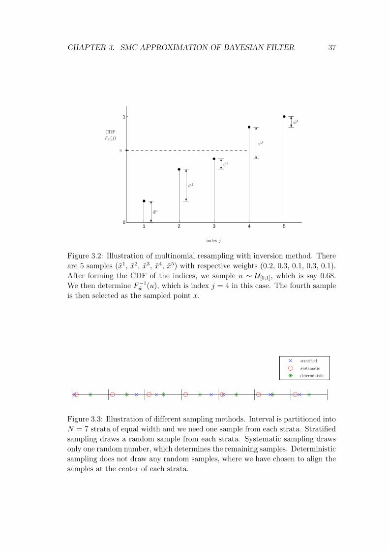
CHAPTER 3. SMC APPROXIMATION OF BAYESIAN FILTER 37
1 2 3 4 50
1
PSfrag replacements
w1
w2
w3
w4
w5
u
index j
CDF
Fw(j)
Figure 3.2: Illustration of multinomial resampling with inversion method. There
are 5 samples (x1, x2, x3, x4, x5) with respective weights (0.2, 0.3, 0.1, 0.3, 0.1).
After forming the CDF of the indices, we sample u ∼ U[0,1], which is say 0.68.
We then determine F−1w (u), which is index j = 4 in this case. The fourth sample
is then selected as the sampled point x.
PSfrag replacements
stratified
systematic
deterministic
Figure 3.3: Illustration of different sampling methods. Interval is partitioned into
N = 7 strata of equal width and we need one sample from each strata. Stratified
sampling draws a random sample from each strata. Systematic sampling draws
only one random number, which determines the remaining samples. Deterministic
sampling does not draw any random samples, where we have chosen to align the
samples at the center of each strata.

CHAPTER 3. SMC APPROXIMATION OF BAYESIAN FILTER 38
drawn are equal to N−∑M
i=1bNwic, which are then obtained by multinomial sam-
pling from xiMi=1 with weights proportional to Nwi − bNwic for i = 1, . . . ,M .
3.4.2 Resampling Schedule
As the resampling is an additional step that is introducing additional approxima-
tions into the algorithm, it has been observed that resampling at every time step
is neither necessary or efficient. For example, Liu and Chen [1998] mention two
such schedules for resampling: deterministic and dynamic. With a determinis-
tic schedule, resampling is performed at fixed intervals while, with a dynamic
schedule, one determines whether to resample or not as the algorithm runs.
This is usually done by computing some value that is meant to be an indicator
of degeneracy and then checking if it is below a predefined threshold.
Effective Sample Size
An indicator of degeneracy was proposed in Kong et al. [1994]. Consider random
MC estimates of the integral of a function f . We denote IN(f) as the classical MC
approximation, assuming it is possible to sample from the distribution of interest,
and IN(f) as the approximation using importance sampling of the form in (3.4).
The ratio of the variances of these two estimates, i.e. Vq[IN(f)]/Vp[I
N(f)], is
suggested to measure the relative efficiency of the importance sampling. The
authors then give an approximation of this ratio as
Vq
[IN(f)
]
Vp
[IN(f)
] ≈ 1 + Vq[ p/q ]. (3.22)
Notice that this approximation conveniently no longer depends on the function
f being integrated.
The approximation of (3.22) is then used to define the effective sample size as
Neff :=N
1 + Vq[ p/q ]=
N
Eq[ (p/q)2 ].
As this cannot be computed exactly, this is further approximated as
Neff :=1
∑Ni=1(w
i)2,
where the wi are the normalized importance weights. In practice, this can be
computed every time step and when it falls below some threshold, resampling is
performed.

CHAPTER 3. SMC APPROXIMATION OF BAYESIAN FILTER 39
Low values of Neff can be useful to indicate inaccurate estimates, but it should
be noted that estimates can be extremely inaccurate with no indication from this
quantity. Such a scenario could occur, for example, if an important mode of P is
missed when sampling from Q [Neal 1998, pg. 8].

Chapter 4
SMC for Personal Positioning
Personal positioning refers to calculating the position coordinates of a mobile
station (MS) using measurements. Much of the motivation for the positioning
of mobile devices stems from a Federal Communications Commission order that
required accurate location information for emergency 911 calls made from mo-
bile phones. The requirements are given in terms of circular error probability
(CEP) so that CEPx = ym means that at least x% of the reported location
solutions are within a y meter radius of the true location. The mandate speci-
fies that for mobile-based positioning, CEP67 = 50m and CEP95 = 150m. Other
applications, such as guidance and navigation, yellow page services, and location-
sensitive billing, are also driving forces for the technology. [Gustafsson and Gun-
narsson 2005]
SMC methods have been proposed for positioning and other related applications,
such as navigation and tracking. In Section 4.1, we give a literature review. We
then present the general concepts of positioning in Section 4.2. Our emphasis is
on the mathematical models to describe the motion of the MS and the measure-
ments from satellite and cellular network based systems. The Bayesian framework
will be essential in our formulation of the positioning problem so that the SMC
methods are applicable. In Section 4.3 and Section 4.4, we give two separate sets
of simulations using SMC.
40

CHAPTER 4. SMC FOR PERSONAL POSITIONING 41
4.1 Literature Review of Related SMC Appli-
cations
SMC has been successfully applied to many related problems, and here we note
some contributions. This literature review is by no means exhaustive, but is
meant to indicate the application-oriented material that was consulted for this
work.
The Department of Electrical Engineering at Linkoping University has been quite
prolific in publishing SMC applications for positioning, navigation, and tracking.
Illustrations of SMC in aircraft navigation can be found in Bergman [1999], Nord-
lund and Gustafsson [2002], Schon et al. [2003], and Nordlund and Gustafsson
[2001]. Gustafsson and Gunnarsson [2003] present a MC technique for static po-
sitioning from time difference measurements and mention that it can be easily
extended to dynamic scenarios. Nordlund et al. [2002] illustrate SMC for po-
sitioning in a wireless network using distance and power measurements, where
velocity is assumed known (e.g. in a car-mounted application). Several of these
applications are also included in the survey, Gustafsson et al. [2002].
Morelande et al. [2003] and Moreland and Challa [2005] present a study of particle
filters in target tracking although there is focus on the data association problem
of tracking in clutter. Ristic et al. [2004] is one of the few books on SMC currently
available and it has a tutorial with a large section of the book devoted to tracking
applications. Similar work can be found in the robot localization applications of
Fox et al. [2001].
4.2 Personal Positioning Background and Prin-
ciples
In this section, we describe the ideas of personal positioning and presents a
Bayesian approach to the problem. To start, recall that we have a signal
process X = (xk)∞k=0, which represents what we intend to estimate. For our
purposes, we define xk, i.e. state of the signal at time k, to consist of a MS
position and velocity component [rk,uk]T per coordinate and will either have 2
or 3 coordinates, i.e. xk ∈ R4 or xk ∈ R
6 respectively.
In Section 4.2.1, we briefly discuss the various signals and measurement mod-
els commonly used in positioning. In Section 4.2.2, we present the positioning
problem for the stationary case and in Section 4.2.3, for the dynamic case. The
dynamic case formulation defines the system equations, (2.9) and (2.10), which
connects the positioning problem to the Bayesian filtering.

CHAPTER 4. SMC FOR PERSONAL POSITIONING 42
4.2.1 Measurements
Positioning relies on measurements that depend on the state of the MS. Re-
call the general form of the measurements used in the system equations (2.10),
i.e. yk = hk(xk) +wk. We will be interested in formulating our measurements
for positioning in this form, where now xk is the MS state.
There are a variety of signals in cellular networks that can be used for position-
ing, see e.g. Syrjarinne [2001]. For example, Time of Arrival (TOA) and Round
Trip Delay (RTD) positioning use propagation times of signals, Received Signal
Strength (RSS) positioning uses measured signal strengths, and Angle of Arrival
(AOA) positioning uses directions of signal arrival. The signal travel time used
in TOA is proportional to the distance between the MS and base station (BS),
so we model these measurements as range measurements, i.e.
hk(xk) = ‖rb − rk‖,
where rb is the known position of a base station. In addition, the coverage area
of a base station, known as a cell, is normally divided into three sectors so that
if the current sector is known, it can be used to assist positioning, see e.g. Sun
et al. [2005]. If available, base station information about the maximum range
of detection can also be incorporated. We may refer to base station sector and
maximum range information as “measurements”.
Satellite based networks have their own signals and measurements, see e.g. Kaplan
[1996]. Measuring signal travel times typically requires a synchronized network.
However, in the GPS, the MS clock is not synchronized to the clocks of the
satellites, which results in an added bias term for the range measurements. These
biased range measurements will be called pseudorange measurements, where
the observation function can be modelled as [Parkinson and Spilker 1996, pg. 410]
hk(xk) = ‖rsk − rk‖ + bk,
where rsk is the known position of a satellite (SV, i.e. space vehicle) at time k and
bk is the unknown, time-dependent bias term. In addition, delta pseudorange
measurements are available, which rely on signal Doppler shifts produced by
the satellite and user motion. The observation function is modelled as [Parkinson
and Spilker 1996, pg. 411]
hk(xk) =(rs
k − rk)T
‖rsk − rk‖
(usk − uk) + bk,
where rsk and us
k are the position and velocity of a satellite at time k respectively,
and bk is an unknown time-dependent bias term.
Since, at a given time step k, the bk bias terms are the same for all pseudorange
measurements and the bk bias terms are the same for all delta pseudorange mea-
surements, we can use differenced measurements to subtract out the bias, see

CHAPTER 4. SMC FOR PERSONAL POSITIONING 43
e.g. Ali-Loytty et al. [2005]. This means that for two satellites s0 and s1 that
can be seen at a time k, the differenced pseudorange measurement uses the
model
hk(xk) = ‖rs1k − rk‖ − ‖rs0
k − rk‖
and the differenced delta pseudorange measurement uses the model
hk(xk) =(rs1
k − rk)T
‖rs1k − rk‖
(us1k − uk) −
(rs0k − rk)
T
‖rs0k − rk‖
(us0k − uk).
Using differenced measurements requires that we have at least two measurements.
It should be noted that a vector of differenced measurements can have correlated
errors.
We will frequently refer to the measurements of this section in our simulations.
Note that the Euclidean norm ‖·‖ is a nonlinear operation so that these observa-
tion functions hk are nonlinear functions of xk.
4.2.2 Static Case
The basic approach to positioning solves the problem at each time step separately
using only measurements from the given time step—hence, we say it is a static
or stationary problem. The measurements that are used are typically only
functions of the MS position and an error term, i.e. yk = hk(rk) +wk. The static
positioning problem is then to find the position that minimizes some loss function
V (rk). Multiple measurements are generally needed to prevent underdetermined
cases with multiple solutions.
Several common choices for loss functions are given in Gustafsson and Gunnarsson
[2005], which we list in Table 4.1. There are special cases where the nonlinear least
squares problem can be reformulated as a linear least squares problem so that
there exists a closed-form solution, see e.g. Smith and Abel [1987]. In general,
however, the solution of these problems requires an iterative numerical search
algorithm, such as a steepest descent or Gauss-Newton method.
Table 4.1: Loss Functions V (rk)
Nonlinear Least Squares (yk − hk(rk))T (yk − hk(rk))
Weighted Nonlinear Least Squares (yk − hk(rk))T Σ−1
wk(yk − hk(rk))
Maximum Likelihood −log pwk(yk − hk(rk))

CHAPTER 4. SMC FOR PERSONAL POSITIONING 44
4.2.3 Dynamic Case
Positioning can also be formulated as a dynamic problem, where, assuming
some motion model, we can use the solution of a given time step to infer knowl-
edge about the solution of the next time step. Incorporating this additional
information should improve the estimates. The dynamic positioning approach
does not require multiple measurements at each time step as the static position-
ing approach does; this could be an important consideration in situations where
measurements are scarce.
There are a wide variety of mathematical models that describe the evolution of
an object’s kinematic state with respect to time, see e.g. Li and Jilkov [2003].
Recall the general form of the signal model used in the system equations (2.9),
i.e. xk = fk−1(xk−1) + vk−1, where now the state of the signal is the position and
velocity of the MS. Note that the choice of motion model defines the signal model.
We will refer to the following model in the simulations of this work. The evolution
of the state in continuous time can be described by a white noise acceleration
model. The discretized state equation for each coordinate is written as
xk = Fk−1xk−1 + vk−1, Fk−1 =
[1 ∆tk0 1
], (4.1)
where ∆tk := tk − tk−1. The signal noise is independent in time and given such
that vk−1 ∼ N (0,Σvk−1) with
Σvk−1=
[13∆t3k
12∆t2k
12∆t2k ∆tk
]γ, (4.2)
where γ is a design parameter. If γ is chosen such that changes in the velocity are
small compared to the actual velocity, then this is called the nearly constant-
velocity model. [Bar-Shalom and Li 1998]
Note that having defined the observation models and signal models for the state
equations of (2.9) and (2.10), then the Bayesian recursions give the optimal so-
lution in the form of a probability distribution, i.e. the posterior. Although the
white noise acceleration model defines a linear and Gaussian signal model, the
observation models are nonlinear, which prevents a tractable form of the poste-
rior. Extended Kalman filtering is a natural approach and is commonly applied
to positioning using satellite measurements [Kaplan 1996]. However, the nonlin-
earity from terrestrial-based measurements can be more severe in which case the
linear approximations made by the EKF are inadequate, see e.g. Ali-Loytty et al.
[2005].
The nonlinear filtering formulation of positioning is ideally suited for SMC. Of
course, the computational and memory requirements for SMC are quite large so

CHAPTER 4. SMC FOR PERSONAL POSITIONING 45
that it might not be currently a feasible solution to implement on a consumer’s
mobile phone. Nonetheless, it is worthwhile to consider the pros and cons of such
an approach, as it will most likely be feasible eventually. At the very least, an
SMC filter could be used as a reference to evaluate the quality of other Bayesian
filters.
4.3 Simulation Set 1: Testbench
We have implemented the particle filter for a positioning testbench—a software
package that generates positioning-style measurements and computes a number of
filter evaluation statistics1. We first present a brief description of the testbench,
followed by two separate simulations using it. In the first set of simulations,
given in Section 4.3.2, we illustrate how the PF performs in different positioning
scenarios. In the next set of simulations, given in Section 4.3.3, we consider how
the choice of importance distribution affects the performance of the filter.
4.3.1 Description
This section describes the models that were used in the simulations. Note that
because we are using simulated data, the correct motion and measurement mod-
els are available for the filters. In any application, these models would have to be
estimated and there would most likely be modelling errors, which then compli-
cates the comparison of different filters. We have not considered modelling errors
in this work.
State and Dynamics
All of the simulations of this section used a position-velocity model with three-
dimensional position and velocity in a local East-North-Up (ENU) reference
frame, i.e.
xk = [ rek rn
k ruk ue
k unk uu
k ]T .
The state’s initial distribution Px0is Gaussian and known. No model is given to
describe how the the bias terms (bk,bk) in the pseudorange and delta pseudorange
measurements evolve in time, so we do not attempt to estimate them; we use
differenced measurements to eliminate the bias terms.
1The positioning testbench software, including data generation and filter evaluation statis-
tics, was designed and implemented by Niilo Sirola, of the Personal Positioning Algorithms
Research Group at Tampere University of Technology.

CHAPTER 4. SMC FOR PERSONAL POSITIONING 46
All simulated trajectories are 120 seconds long with time steps of one second.
The signal model function is linear, time-invariant, and defined by the matrix
F =
1 0 0 1 0 0
0 1 0 0 1 0
0 0 1 0 0 1
0 0 0 1 0 0
0 0 0 0 1 0
0 0 0 0 0 0.9
.
The signal noise is independent in time and is modelled as Gaussian with zero
mean and covariance given by (4.2) with γ equal to 2 m2/s3 for north and east
directions and 0.1 m2/s3 for the up direction. Note that this resembles the white
noise acceleration model mentioned in Section 4.2.3 but the 0.9 term in the F
matrix is a heuristic to restrict motion in the vertical direction. We use this
heuristic of the testbench without justification, but note that the data is simulated
so for our purposes, it is important only that the filters use the same models that
generated the data.
Measurements
The testbench simulates the measurements mentioned in Section 4.2.1: range,
pseudorange, delta pseudorange, sector, and maximum range. The range, pseu-
dorange, and delta pseudorange measurements have an additive error term,
which is independent for each measurement and is independent in time. The
errors are modelled as Gaussian with zero-mean and a known scalar variance σ2,
i.e. wk ∼ N (0, σ2). Positions and velocities of satellites are based on real data,
measured on the Tampere University of Technology campus on June 18, 2003.
The base station positions are simulated and are placed on a hexagonal grid on
the local East-North plane.
There are five different positioning scenarios that were explored with the test-
bench, see Table 4.2 for their general characteristics. Note that at a given time
step, a base station may report a range measurement, information concerning the
Table 4.2: Measurement Availability for Different Test Cases
Case 1 2 3 4 5
BS low high med med none
Sectors no no no yes no
SV none none low med high

CHAPTER 4. SMC FOR PERSONAL POSITIONING 47
maximum range of detection, and possibly sector information, while a satellite
may report a pseudorange and a delta pseudorange measurement.
4.3.2 Multiple Trajectories: EKF vs PF at Different Sam-
ple Sizes
From each positioning environment given in Table 4.2, we simulate 100 different
trajectory realizations, each with a corresponding measurement realization, and
run the PF once on each set of measurements. Evaluation statistics are computed
over each separate positioning environment so that we can get a general idea of
how the PF behaves in the different environments. See Table 4.3 for details on
the generated measurements.
This set of simulations was intended to give a “system level” perspective of the
PF performance where the details of individual trajectories are intentionally left
unanalyzed. Later simulations will look at the PF performance in closer detail.
Evaluation Criteria
We will now present a brief description of the evaluation criteria used in this set
of simulations. All of the computed statistics use only the East-North position di-
mensions. The Euclidean distance between the filter mean estimates and the true
track is calculated at every time step and the average of these errors is referred to
as “Mean error [m]”. The “95% error [m]” statistic shows the distance that 95%
of the errors were within, while “Inside 50m [%]” and “Inside 150m [%]” gives
Table 4.3: Testbench Cases
Case 1 2 3 4 5
# of BS 0 − 3 0 − 5 0 − 4 0 − 4 0
% of time with # BS > 1, 2 27.1, 2 67.7, 21.3 40.1, 3.8 44.7, 7.4 −σrange [m] 100 100 100 100 −# of sectors 1 1 1 3 −Cell radius [km] 1.5 1 2 2 −
# of SV 0 0 0 − 4 0 − 4 1 − 6
% of time with # SV > 1, 2 − − 55.2, 23.4 69.8, 41.9 94.3, 65.2
σpseudorange [m] − − 10 − 30 8 − 30 8 − 20
σdelta pseudorange [m/s] − − 1 − 4 1 − 3 1 − 2

CHAPTER 4. SMC FOR PERSONAL POSITIONING 48
the percentage of time steps that the filter estimates were within the specified
range. The “Yield [%]” statistic gives the percentage of trajectories that the fil-
ter was able to complete successfully. The PF might not be able to complete
a trajectory successfully if all the samples are in an insignificant region of the
state-space and the importance weights sum to zero; in this case, the weights
cannot be normalized due to the division by zero and the filter cannot continue.
Tested Filters
Only one choice of importance distribution for the PF is considered here, along
with an EKF. As we have claimed that the approximations made by the EKF
may be inadequate in a number of cases, it is worthwhile to include EKF results
for comparison. The EKF does not use the base station sector or maximum range
information since they are not linear and Gaussian measurements and it is not
straightforward to incorporate the information in this filter. On the other hand,
the PF simply incorporates this information with the weight updates, i.e. if a
given sample is outside of the reported sector or beyond the maximum range of
detection, then it is assigned zero weight.
The PF samples from the empirical prediction distribution, i.e. we use the SIR1
filter. Systematic sampling is used to draw M = N samples from the importance
distribution at every step, and the final resampling step is skipped. We have run
the PF using a number of different sample sizes: 102, 103, 104, 105, 106, 2 · 106.
The largest sample sizes was around where the computational complexity began
to be a burden.
The intention of this set of simulations is as follows. The quality of the PF
approximations of the posterior should improve with larger sample sizes and
should degrade with smaller sample sizes. Correspondingly, we expect the quality
of the filter estimates to improve with larger sample sizes and degrade with smaller
sample sizes. If an increase of sample size does not change the filter results, then
we can be confident that we have a sufficient number of samples to adequately
represent the posterior distributions. On the other hand, if the filter results
continue to change as we increase the sample size, then we cannot be sure if the
results would continue to change at even larger sample sizes. The main idea of
this simulation is to repeat this analysis for the different positioning scenarios
and determine which environments present more difficulty for the PF.
Results
The simulation results for each positioning environment are presented separately
in Table 4.4. First, notice that there is not much difference between the filters

CHAPTER 4. SMC FOR PERSONAL POSITIONING 49
considering the “Inside 50m [%]” and “Inside 150m [%]” criteria. Although it
is perhaps interesting to compare these numbers for the different test cases, it
does not emphasize the difference between the filters for a given test case. The
“Yield [%]” results were included to indicate the few times that the small sample
PFs could not continue. The comments of this section will focus on the results
for the two remaining criteria, “Mean error [m]” and “95% error [m]”.
Let us first compare the PF at different sample sizes. In general, the PF results
seem to be converging to specific values as the sample size increases. It is re-
assuring that the results of all test cases do not change significantly after, say
104 samples. For a personal positioning application, this difference would most
likely be irrelevant and the larger number of samples would not be necessary. On
the other hand, from the point-of-view of approximating the optimal filter, it is
disturbing that for some cases, the “95% error [m]” results continue to change
as the sample size increases. For Cases 2 and 4, the results stabilize relatively
quickly (104 samples), while Case 1 needed much more samples (106 samples).
The results for Cases 3 and 5 do not indicate that there are sufficient samples for
this behavior.
Care should be taken when interpreting the results from the PFs with smaller
sample size; if increasing the sample size changes the results, then repeating
the experiment with the same sample size could also change the result. As an
example, different realizations of the “95% error [m]” result for the Case 2 data at
a sample size of 103 gave 185, 185, 175, 190, and 182 m. This randomness explains
the nonintuitive scenario when there are smaller errors for smaller sample sizes
which, of course, is not indicative of better performance.
The fact that the PF seems to require a large number of samples for Case 5 is
peculiar since this case uses only satellite measurements, which are more accurate
than the base station data. This oddity was due to trajectories in which there
were no more than two satellites seen at each step. Such a scenario can result in
narrow distributions that can grow quite large, which then require a large number
of samples for a good approximation. This will be looked at in the next section.
The scenarios when the PF outperformed the EKF are not surprising: the differ-
ence is most visible in the noisy and highly nonlinear scenarios of Case 1 and 3,
with no apparent difference for the satellite-only measurements of Case 5.
To make conclusions about the PF performance in specific scenarios, we can say
the following. With fewer measurements, the PF behaves more unpredictably
and could require a large number of samples (see Cases 1 and 3). Also, the use
of maximum range and sector information from base stations could be useful for
the PF (compare Cases 4 and 5). Finally, the more nonlinear and noisy scenarios
should show more of an improvement of the PF over the EKF.

CHAPTER 4. SMC FOR PERSONAL POSITIONING 50
Table 4.4: Simulation Results for Cases 1-5
Case 1 PF EKF
Sample size 102 103 104 105 106 2 · 106 —
Mean error [m] 231 217 211 213 213 213 242
95% error [m] 837 801 743 748 754 754 982
Inside 50m [%] 21.8 25.6 24.9 25 24.9 24.9 25.8
Inside 150m [%] 55.2 59.2 58.1 58.2 58 58 59.2
Yield [%] 88 99 100 100 100 100 100
Case 2 PF EKF
Sample size 102 103 104 105 106 2 · 106 —
Mean error [m] 75.7 70.3 67.7 68 67.9 68 75.7
95% error [m] 200 191 181 182 182 182 206
Inside 50m [%] 43.1 46.2 47.3 47 47.2 47.2 46.2
Inside 150m [%] 90.3 91.7 92.4 92.5 92.5 92.5 90.8
Yield [%] 90 100 100 100 100 100 100
Case 3 PF EKF
Sample size 102 103 104 105 106 2 · 106 —
Mean error [m] 113 97.4 94.2 95.7 95.1 95.3 117
95% error [m] 437 389 398 406 410 407 493
Inside 50m [%] 52.7 59.3 59.7 60 60.1 60 60.2
Inside 150m [%] 83.7 87.8 87.2 87 87 87 87.9
Yield [%] 96 100 100 100 100 100 100
Case 4 PF EKF
Sample size 102 103 104 105 106 2 · 106 —
Mean error [m] 55.7 43.6 42.6 42.2 42.2 42.1 48.6
95% error [m] 138 128 118 117 118 118 134
Inside 50m [%] 70.9 75.7 76.7 77.1 77 77.1 75.9
Inside 150m [%] 95.6 96 96.7 96.7 96.7 96.7 95.7
Yield [%] 87 98 100 100 100 100 100
Case 5 PF EKF
Sample size 102 103 104 105 106 2 · 106 —
Mean error [m] 61.8 60.6 59 57 57.6 57.5 57.6
95% error [m] 260 270 256 259 260 262 263
Inside 50m [%] 75.6 80.2 80.8 81.1 81.1 81.3 81.2
Inside 150m [%] 91.5 91.7 91.7 91.7 91.6 91.7 91.8
Yield [%] 98 100 100 100 100 100 100

CHAPTER 4. SMC FOR PERSONAL POSITIONING 51
4.3.3 Comparing PFs with Different Importance Distri-
butions
As the PF relies on random simulations, the estimates conditioned on a real-
ization of the observation process are random. This is in contrast with, e.g. an
EKF, which forms an estimate that is deterministic conditioned on the realized
measurements. PF performance can be evaluated by filtering one realization of
the observation process multiple times and analyzing how the estimates vary over
different realizations of the algorithm, i.e. the MC variation of the filter. Better
PFs vary less. In this set of simulations, we will be interested in the MC variation
of the PF mean estimates, and more specifically, comparing this MC variation
from PFs using different importance distributions.
One trajectory and a Case 5 set of measurements was generated so that there
are only satellites measurements, i.e. pseudoranges and delta pseudoranges. In
Figure 4.1(a), the trajectory realization is plotted in the East-North plane along
with the PF estimates from one realization of the algorithm. This set of mea-
surements was a rare case in that there are no more than two satellites seen at
each time step; the filters then have no more than one differenced pseudorange
measurement and one differenced delta pseudorange measurement at each time
step. This causes the significant region of the likelihood function to be quite
narrow, which in effect, causes the significant region of the posterior distribution
to be narrow also and to “stretch out” as time progresses from the uncertainty
in the dynamic model.
This set of measurements was chosen for two reasons. First, we wanted to illus-
trate the scenario that can occur when the Bayesian mean does not resemble the
true track. Notice how the true track veers to a northern direction while the filter
mean estimates continue eastward. Intuitively, one might want to compare the
filter estimates with the true track and claim that the “better” filter is the one
giving estimates closer to the true track. We must keep in mind that the “better”
Bayesian filter is the one that gives a closer approximation of the true Bayesian
solution, and is not necessarily the filter that has an estimate closer to the true
track. Cases such as this complicate the comparison of different Bayesian filters
because we do not know the true Bayesian solution so we must evaluate how close
the filters approximate a value we do not know.
The second reason that this set of measurements was chosen was to illustrate
the MC variation of the PF estimates. A PF was run 500 times on this set of
measurements and we have plotted the covariances of the filter mean estimates
as 3σ ellipses in Figure 4.1(b), which is a close-up of the subregion box in Fig-
ure 4.1(a). These ellipses characterize the MC variation that more elaborate PFs
should reduce. The ellipses are quite narrow so that it is convenient to only look
at the ellipse major-axis vertices; lines through every time step’s ellipse vertices

CHAPTER 4. SMC FOR PERSONAL POSITIONING 52
are drawn in Figure 4.1(c).
We should point out that in computing the covariance of the mean estimate, we
are using the ensemble average (the average over the algorithm realizations) in
place of the unknown true Bayesian mean. Many simulations in the literature have
used the true track in place of the true Bayesian mean, which of course, would
not be appropriate here. Similar results were obtained by using an estimate of
the true Bayesian mean from a large sample SIR1 PF, e.g. at 106 and 107.
The different importance distributions tested include the four examples from
Section 3.3.2, i.e. SIR1, SIR2, SIR3, and SIR4. All the SMC methods used
systematic resampling to simulate M = N = 104 samples from the importance
distribution at every step, and skipped the final resampling step. The effectiveness
of the different importance distributions is illustrated in Figure 4.1(d). Each
successive filter shows an improvement over the previous, i.e. SIR2 was better
than SIR1, SIR3 was better than SIR2, etc. These improvements can be compared
with an SIR1 PF with larger sample sizes in Figure 4.1(e).
The improvement of the different importance distributions is slight. One mo-
tivation for the construction of an importance distribution based on local lin-
earizations is for very accurate sensors, i.e. peaked likelihoods, see e.g. van der
Merwe et al. [2000, pg. 2]. Considering the types of measurements available in
our scenarios, the satellite measurements are the more accurate ones and the base
station measurements are noisier. We should expect even less of an improvement
with only base station data. Peaked likelihoods could also result from many
measurements received at a given time step, but we are less concerned with such
situations because a static positioning solution could then be appropriate, see
Section 4.2.2. Another motivation for the linearizations is for data that under-
goes sudden changes, see e.g. van der Merwe et al. [2000, pg. 2]; this subject was
not considered in this work.

CHAPTER 4. SMC FOR PERSONAL POSITIONING 53
PSfrag replacementsnorth
east
k = 0
1km
true track
filter mean and covariance
subregion
(a)
PSfrag replacements
200m
mean realizations
ensemble average
covariance ellipse
true track
(b)
PSfrag replacements
200m
covariance ellipse
true track
line through ellipse major-axis vertices
(c)
PSfrag replacements
200m
SIR4SIR3
SIR2
SIR1
true track
(d)
PSfrag replacements
200m
N = 104
N = 105
N = 106
true track
(e)
Figure 4.1: (a) PF estimates from one realization of the algorithm. (b) Subregion
of (a) showing a number of mean realizations and covariance of mean estimates.
(c) Envelope characterizing the covariance ellipses. (d) Comparison of different
importance distributions at a sample size of 104. (e) Comparison of SIR1 at
different sample sizes. All covariance ellipses are 3σ contours and are plotted at
30 second intervals.

CHAPTER 4. SMC FOR PERSONAL POSITIONING 54
4.4 Simulation Set 2: Comparing PF Posterior
Approximations
In the literature, many PF simulations focus on the MC variation of the mean
estimates, i.e. the randomness introduced by the MC algorithm that can be ob-
served from the empirical mean estimates. In this section, we develop a method
to compare PF performance that uses the distribution approximation itself rather
than a single estimate formed from it.
A distribution analysis could be more useful than an estimate analysis. As ex-
amples, two filters could give similar mean estimates although one of them has a
distribution “closer” to the true distribution. Also, in a bimodal case, the mean
could be between the two modes in a region of the state-space where there is
little probability of the target being located; in a case such as this, the mean is
less interesting to analyze. We will discuss some of the background related to
comparing distributions and then apply these methods to the comparison of the
particle filters.
4.4.1 Comparing Distributions with χ2-tests
The comparison of distributions from empirical data is an established branch of
statistics with applications in numerous fields. These techniques are primarily
hypothesis tests. This involves computing a test statistic which, under some
assumed hypothesis, should have a certain distribution. If the computed statistic
falls outside a given confidence region of the assumed distribution, the hypothesis
is rejected and is not rejected otherwise. [Bar-Shalom and Li 1998]
The chi-squared (χ2) test is one such procedure for distribution comparisons,
see e.g. Cochran [1952] or Moore [1986] for an overview. When comparing em-
pirical data with a known distribution, the idea relies on grouping the n ob-
served data samples into B mutually exclusive bins and forming a hypothesis
that states the probability pj that an observed data point will fall into the jth
bin, for j = 1, . . . , B. To check this hypothesis, the following quantity is used
[Cochran 1952]
ψ =B∑
j=1
(oj − ej)2
ej
,
where oj is the observed number of samples in the jth bin and ej is the expected
number of samples for the jth bin, i.e. ej = n pj. Pearson showed in 1900 that if
the hypothesis is true and n is large, then the distribution of the test statistic ψ
is approximately χ2 with B − 1 degrees of freedom (χ2B−1) [Cochran 1952].

CHAPTER 4. SMC FOR PERSONAL POSITIONING 55
The idea can be extended from comparing empirical data with a known distribu-
tion to comparing two sets of empirical data with each other. In this case, the
hypothesis is that the two samples are from a common distribution. The form of
the computed test statistic is [Baggerly 2001]
ψ =2∑
i=1
B∑
j=1
(oij − eij)2
eij
, (4.3)
where oij is the observed count of the jth bin of the ith sample set and eij is the
expected count of the jth bin of the ith sample set given by
eij = ni(o1j + o2j)
(n1 + n2),
where ni is the number of samples in set i.
A convenient aspect of the χ2-test is that it has a natural extension to multivariate
scenarios. The difficult part is the construction of the bins. The simplest approach
would divide the state-space into a number of equally sized bins, but this can be
computationally difficult for large dimensions, i.e. a large number of bins, most
of which are empty. Choosing bins of unequal size that depend on the data is
a solution. This results in smaller sized bins, hence more resolution, in regions
where more data is expected and larger bins, hence coarse resolution, where less
data is expected. This is known as adaptive or data-dependent binning and
has been discussed in the literature, see e.g. Baggerly [2001, pg. 142] for a brief
overview.
4.4.2 Probability Binning
An interesting application of these ideas in the field of cytometry was given by
Roederer et al. [2001]. Test samples, i.e. sets of multidimensional data, are to
be ranked according to their similarity to a control sample, which is a sample of
data chosen to represent some known behavior. A multivariate data-dependent
binning technique was proposed that adaptively constructed bins according to the
control sample, followed by the use of a test statistic to quantify the difference
between the test and control sample. Baggerly [2001] provides a more theoreti-
cal discussion with the recommendation to use the standard two-sample χ2-test
statistic (4.3).
The algorithm for constructing the bins, called probability binning, is quite
simple and is as follows. The variance of the control sample along each of the d
dimensions is computed and the dimension with the largest variance is chosen to
be divided. The sample median value of the chosen dimension is then chosen as
the point at which to partition the state-space in two. This is then repeated for

CHAPTER 4. SMC FOR PERSONAL POSITIONING 56
each partitioned subspace, continuing until the desired number of bins has been
reached. The result is a set of d-dimensional hyper-rectangular bins with sides
parallel to the coordinate axes and each bin containing roughly the same number
of control samples, see Figure 4.2. Assuming then, that a test sample is from
the same distribution as the control sample, each bin will roughly have the same
expected frequency.
Example
This simple example illustrates the idea of probability binning and comparing
distributions using the two-sample χ2-test statistic. We use 106 samples from a
standard Gaussian distribution in R4 as the control sample to partition the state-
space into B = 64 bins. Test samples, each of 104 samples, are then generated
from the same distribution, binned, and scored. Since all the test samples are
from the same distribution as the control sample, we expect the realized test
scores to follow the theoretical χ2B−1 distribution quite well. This can be verified
in Figure 4.3, where we plot the histogram of the realized test scores along with
the theoretical density.
4.4.3 Application to Linear and Gaussian Filtering Sce-
narios
In this section, we apply the probability binning to a simple filtering scenario.
Assume for a moment, that we are able to generate IID samples from the true
marginal posterior πk|k. We can then apply the procedure in Section 4.4.2 at
each time step so that the state-space Rnx is partitioned into bins using a sample
from the true marginal posterior. It might be reasonable then to assume that
the quality of a PF approximation of πk|k can be assessed using the two-sample
χ2-test, where the hypothesis is that the samples from the true marginal posterior
and the samples from the PF approximation are from the same distribution.
Roughly speaking, we might expect better PFs to give better test scores, where
“better test scores” refers to realizations of a random variable with distribution
closer to the assumed χ2 distribution. We check this empirically by repeating the
simulation 1000 times and comparing the mean and variance of the realized test
scores to that from the assumed χ2 distribution. For a χ2B−1 distribution, the
mean is B − 1 and the variance is 2 · (B − 1).
To verify that the test score analysis is meaningful, we will compare our conclu-
sions to those made from a root mean square error (RMSE) analysis of the

CHAPTER 4. SMC FOR PERSONAL POSITIONING 57
Figure 4.2: Probability binning in R2 with B = 32
20 30 40 50 60 70 80 90 100 110 1200
0.01
0.02
0.03
0.04
PSfrag replacements
Figure 4.3: Simple test with standard Gaussian distribution in R4 with B = 64.
(Scaled) Histogram of empirically realized test scores (104 realizations). Density
of χ2B−1 distribution is shown in red. All test samples used 104 samples and the
control sample used 106 samples.

CHAPTER 4. SMC FOR PERSONAL POSITIONING 58
mean estimates. The RMSE is given as
RMSEk =√
E [ ‖ µk − µk ‖2 ], (4.4)
where µk is the random posterior mean estimate and µk is the true posterior
mean. The expectation in (4.4) is approximated by repeating the simulation 500
times and using the sample mean.
The binning of the PF samples is done as follows. At each time step, we sim-
ulate M = N = 104 samples using multinomial sampling from the importance
distribution, evaluate weights, and skip the final resampling step. The binning at
each time step uses the weighted samples. We draw 104 samples using systematic
resampling from this weighted discrete distribution, bin the equally-weighted sam-
ples, compute the test score, and discard these resampled points. If the weights
are equal, which is the case for SIR4 in the linear and Gaussian scenario, then
the binning can proceed without resampling.
Simulation
For this simulation, the state is in R4 with two position coordinates and two
velocity coordinates, i.e.
xk = [ rek rn
k uek un
k ]T .
We simulate a 200 second trajectory from a white noise acceleration model with
a constant time step of 1 second and γ = 3 m2/s3. The state’s initial distribution
Px0is Gaussian and known. One measurement is produced every time step and
is modelled as
yk =
[1 0 0 0
0 1 0 0
]xk +wk, wk ∼ N (
[0
0
],
[σ2 0
0 σ2
]).
As this filtering problem is linear and Gaussian, the marginal posterior distribu-
tion at each time step is Gaussian and can be computed with the Kalman filter.
In this case, we can then draw samples directly from the marginal posterior to
use as a control sample to partition the state-space. A particle filter can then be
run on the data, where at every time step, we bin the samples and compute test
scores. Of course, this is just for illustrative purposes because the Kalman filter
solves the problem exactly and there is no reason to resort to particle filtering.
We again test the four PF examples of Section 3.3.2, i.e. SIR1, SIR2, SIR3,
and SIR4. Note that this is a special case for SIR3 and SIR4 since there is
no need for linearization. All filters sampled M = N = 104 samples from the
importance distribution and skipped the final resampling step. For each filter,

CHAPTER 4. SMC FOR PERSONAL POSITIONING 59
four separate simulations were run, each using a different variance σ2 for the noise
in the measurement model: 104, 25, 1, 0.1 m2.
The mean and variance of the test scores at a single time step are given in
Table 4.5. It is interesting to note that the test scores rarely resemble the χ2 the-
oretical distribution. In fact, this occurs only with the SIR4 filter in the σ2 = 1
and 0.1 m2 cases. However, there appears to be different behavior for the different
filters. For cases with larger measurement noise variances (σ2 = 104 and 25 m2),
the two filters using alternative weights in the importance distribution (SIR2 and
SIR4) have smaller means and variances. For cases with smaller measurement
noise variances (σ2 = 1 and 0.1 m2), the two filters using alternative components
in the importance distribution (SIR3 and SIR4) show smaller means and vari-
ances, while the SIR2 results behave erratically. It might be reasonable then to
conclude that the filters having test scores closer to the theoretical distribution
χ2B−1, i.e. having smaller test score means and variances, are working better.
Similar results, concerning the score mean, can be seen in Figure 4.4, where
the score mean is plotted over the whole simulation. Note that all the results
are rather similar with large σ2, and the differences become more apparent as
σ2 decreases. Also note that in Figure 4.4(a) and Figure 4.4(b) there is near
identical results for the SIR1 and SIR3 filters and for the SIR2 and SIR4 filter.
In Figure 4.4(d), the SIR2 score means are quite large and are outside of the
plotted region. The intention of these plots was not to display the actual score
means, but instead to show relative performance of the different filters.
Table 4.5: Mean and variance of two-sample χ2-test statistic for linear-Gaussian
scenario at time step k = 180 with number of bins B = 64.
σ2 = 10000 m2 χ2 SIR1 SIR2 SIR3 SIR4
Mean 63 781 611 784 611
Variance 126 4.02 · 104 2.69 · 104 4.40 · 104 2.49 · 104
σ2 = 25 m2 χ2 SIR1 SIR2 SIR3 SIR4
Mean 63 245 119 237 104
Variance 126 2823 586 2847 416
σ2 = 1 m2 χ2 SIR1 SIR2 SIR3 SIR4
Mean 63 276 730 152 66
Variance 126 2561 5.32 · 106 705 138
σ2 = 0.1 m2 χ2 SIR1 SIR2 SIR3 SIR4
Mean 63 929 2.65 · 104 112 64
Variance 126 2.94 · 104 2.30 · 109 394 138

CHAPTER 4. SMC FOR PERSONAL POSITIONING 60
We now consider an analysis of the RMSE of the mean estimates. The RMSE
values are divided by the SIR1 RMSE values and plotted in Figure 4.5. These
relative RMSE values show how the MC variation of mean estimates for the differ-
ent filters compare to SIR1: values lower than one indicate improved performance
compared to SIR1 (less MC variation) while values above one indicate worse per-
formance (more MC variation). With the largest noise variance (σ2 = 104 m2),
all the filters seem to have similar MC variance. With σ2 = 25 m2, the SIR2 and
SIR4 filters clearly have less MC variation, while for cases with smaller measure-
ment noise variance (σ2 = 1 and 0.1 m2), the SIR3 and SIR4 filters have less MC
variance. Also, the SIR2 behaves erratically at the smaller measurement noise
variance.
In summary, similar conclusions about the relative performance of the different
PFs can be found using alternative criteria, i.e. the distribution analysis and the
RMSE analysis of the mean estimates. The usefulness of this distribution analysis
is limited because we required an analytic form of the marginal posterior. In
Section 4.4.4, we extend the analysis to the general filtering scenario.

CHAPTER 4. SMC FOR PERSONAL POSITIONING 61
SIR1SIR2SIR3SIR4
PSfrag replacements
00
1000
2000
3000
4000
5000
20 40 60 80 100 120 140 160 180 200
time [s]
mean
(a) σ2 = 10000 m2
PSfrag replacements
00
1000
2000
3000
4000
5000
20 40 60 80 100 120 140 160 180 200
time [s]
mean
(b) σ2 = 25 m2
PSfrag replacements
00
1000
2000
3000
4000
5000
20 40 60 80 100 120 140 160 180 200
time [s]
mean
(c) σ2 = 1 m2
PSfrag replacements
00
1000
2000
3000
4000
5000
20 40 60 80 100 120 140 160 180 200
time [s]
mean
(d) σ2 = 0.1 m2
Figure 4.4: Mean of two-sample χ2-test statistic for linear-Gaussian scenario

CHAPTER 4. SMC FOR PERSONAL POSITIONING 62
PSfrag replacements
rel.
RMSE
SIR1SIR2SIR3SIR4
00
1
2
20 40 60 80 100 120 140 160 180 200
time [s]
(a) σ2 = 10000 m2
PSfrag replacements
rel.
RMSE
00
1
2
20 40 60 80 100 120 140 160 180 200
time [s]
(b) σ2 = 25 m2
PSfrag replacements
rel.
RMSE
00
1
2
20 40 60 80 100 120 140 160 180 200
time [s]
(c) σ2 = 1 m2
PSfrag replacements
rel.
RMSE
00
1
2
20 40 60 80 100 120 140 160 180 200
time [s]
(d) σ2 = 0.1 m2
Figure 4.5: Relative RMSE with respect to SIR1 for linear-Gaussian scenario
CHAPTER 4. SMC FOR PERSONAL POSITIONING 63
4.4.4 Application to General Filtering Scenarios
We would like to apply this distribution analysis to PFs in the general filtering
scenario where we do not have an analytic form for the posterior. The difficulty is
then to determine a control sample that can be used to partition the state-space.
Ideally, we would have some algorithm that was known to produce IID samples
from the marginal posterior that we could use to produce the control sample. In
the absence of such an ideal algorithm, we have chosen one PF algorithm as the
reference and proceed with the analysis.
The partitioning of the state-space using a reference PF is done as follows. We
have used the SIR3 importance distribution and, at each time step, drawM = 107
samples from the importance distribution, evaluate weights, and then resample
N = 104 samples from this weighted distribution. The importance sampling
uses deterministic sampling (103 samples from each mixture component) and the
resampling uses systematic sampling. The binning at each time step uses the M
weighted samples. We draw 106 samples from this weighted discrete distribution,
perform the probability binning on these equally-weighted samples, and discard
these resampled points. It does seem perhaps more elegant to instead use the N
equally-weighted samples to form the bins, but using a small number of points
in the control sample (relative to the number of points of the test samples) was
noticed to affect the test score distribution, see Figure 4.6.
Our choice of using SIR3 instead of SIR4 for the reference PF deserves discussion
and our reasoning was as follows. A mixture distribution covers the same region
of the state-space regardless of what the mixture weights are. Better weights of
the mixture may result in a more efficient sampler, i.e. a smaller sample size N
is needed for a good approximation; however, a large sample M from the un-
weighted mixture, where M is much larger than N , is inefficient but should give
approximations that are just as good, if not better. In addition, the alternative
weights in SIR2 caused erratic behavior for the small measurement noise scenar-
ios, so it was decided to be cautious and not use any alternative weights in the
reference PF.
We repeat the experiments of Section 4.4.3 but now use a PF approximation of
the posterior as the control sample. It should be mentioned that the simulation
scenario of this section is the same simulation scenario as that in Heine [2005],
i.e. the same signal and measurement models and the same realized measurement
and signal process. We have reproduced the relative RMSE plots of that publi-
cation here for convenience. The contribution of this work is the application of
the probability binning method to the comparison of the PFs.

CHAPTER 4. SMC FOR PERSONAL POSITIONING 64
20 30 40 50 60 70 80 90 100 110 1200
0.01
0.02
0.03
0.04
(a) N = 107
20 30 40 50 60 70 80 90 100 110 1200
0.01
0.02
0.03
0.04
(b) N = 106
20 30 40 50 60 70 80 90 100 110 1200
0.01
0.02
0.03
0.04
(c) N = 105
20 30 40 50 60 70 80 90 100 110 1200
0.01
0.02
0.03
0.04
(d) N = 104
Figure 4.6: Same example as in Section 4.4.2, but now using different number
of samples N for the control sample. (Scaled) Histogram of empirically realized
test scores (104 realizations). Density of χ2B−1 distribution is shown in red. All
test samples used 104 samples.

CHAPTER 4. SMC FOR PERSONAL POSITIONING 65
Simulation
We use the same signal model and realized signal process as the simulation in
Section 4.4.3, but now use range measurements. It is the nonlinearity of the range
measurements that is the distinguishing feature of this set of simulations and that
prevents the posterior distribution from having an analytical form.
The range measurements are of the form
yk = ‖rb − rk‖ +wk, wk ∼ N (0, σ2),
where rb is the known position of a base station. Three base stations are used
and, at each time step, one base station produces a range measurement. In the
simulation of the observation process, the probability of a base station producing
a measurement is inversely proportional to the squared distance to the target.
Again, for each filter, four separate simulations were run, each using a different
variance σ2 for the noise in the measurement model: 104, 25, 1, 0.1 m2. We
repeat the experiments of Section 4.4.3 and present χ2 results along with relative
RMSE plots. The true posterior mean µk in the RMSE analysis, see (4.4), is
approximated using the same reference PF that was used for creating the bins.
We first consider the χ2 results. Due to weights summing to zero in the PF
algorithm on the σ2 = 0.1 m2 case, the SIR1 results used only 995 realizations
and the SIR2 results used only 711 realizations for that case. Comparing Table 4.5
and Table 4.6, it is disturbing that the mean and variance values of the test scores
in the nonlinear scenario are larger than those in the linear scenario. This could
be due to the poor approximation of the true posterior, i.e. the reference PF. If
we compare the relative performance of the different nonlinear filters, i.e. which
filters have the smaller test score means and variances, then the conclusions are
familiar: SIR3 and SIR4 have smaller means and variances for cases with smaller
σ2, SIR2 and SIR4 have smaller means and variances for cases with larger σ2,
and SIR2 is unpredictable for cases with smaller σ2.
Similar results, concerning the score mean, can be seen in Figure 4.7, where the
score mean is plotted over the whole simulation. Again, note that in Figure 4.7(a)
and Figure 4.7(b) there is near identical results for the the SIR1 and SIR3 filters
and for the SIR2 and SIR4 filter and in Figure 4.7(d), the SIR2 results are outside
of the plotted region.
We now consider the RMSE results, which are given in Figure 4.8. Due to weights
summing to zero in the PF algorithm on the σ2 = 0.1 m2 case, SIR1 is averaged
over only 998 realizations and SIR2 is averaged over only 365 realizations for that
case. Comparing these results to those from the linear scenario in Figure 4.5, the
results are similar although the RMSE estimates are noisier, which again could
be due to the poor approximation of the true posterior. The RMSE results of

CHAPTER 4. SMC FOR PERSONAL POSITIONING 66
the nonlinear scenario illustrate that all the filters have similar MC variation for
σ2 = 104 m2, SIR2 and SIR4 have less MC variation for σ2 = 25 m2, SIR3 and
SIR4 have less MC variation for σ2 = 1 and 0.1 m2, and SIR2 is unpredictable
for σ2 = 0.1 m2.
To summarize, our conclusions from the χ2-test are similar to those from the
RMSE analysis. The empirical comparison of different PFs using χ2 techniques
seems to be feasible, even in scenarios where the state-space partitioning relies
on a PF.
Table 4.6: Mean and variance of two-sample χ2-test statistic for nonlinear-
Gaussian scenario at time step k = 180 with number of bins B = 64.
σ2 = 10000 m2 χ2 SIR1 SIR2 SIR3 SIR4
Mean 63 1000 890 1004 890
Variance 126 9.46 · 104 7.14 · 104 8.95 · 104 6.78 · 104
σ2 = 25 m2 χ2 SIR1 SIR2 SIR3 SIR4
Mean 63 349 259 346 254
Variance 126 9.09 · 103 4.44 · 103 1.02 · 104 4.09 · 103
σ2 = 1 m2 χ2 SIR1 SIR2 SIR3 SIR4
Mean 63 456 825 347 213
Variance 126 1.52 · 104 1.63 · 106 9.73 · 103 2.67 · 103
σ2 = 0.1 m2 χ2 SIR1 SIR2 SIR3 SIR4
Mean 63 1050 2.87 · 104 406 269
Variance 126 1.07 · 105 1.76 · 109 1.25 · 104 5.18 · 103

CHAPTER 4. SMC FOR PERSONAL POSITIONING 67
SIR1SIR2SIR3SIR4
PSfrag replacements
00
1000
2000
3000
4000
5000
20 40 60 80 100 120 140 160 180 200
time [s]
mean
(a) σ2 = 10000 m2
PSfrag replacements
00
1000
2000
3000
4000
5000
20 40 60 80 100 120 140 160 180 200
time [s]
mean
(b) σ2 = 25 m2
PSfrag replacements
00
2000
4000
6000
8000
10000
20 40 60 80 100 120 140 160 180 200
time [s]
mean
(c) σ2 = 1 m2
PSfrag replacements
00
2000
4000
6000
8000
10000
20 40 60 80 100 120 140 160 180 200
time [s]
mean
(d) σ2 = 0.1 m2
Figure 4.7: Mean of two-sample χ2-test statistic for nonlinear-Gaussian scenario

CHAPTER 4. SMC FOR PERSONAL POSITIONING 68
PSfrag replacements
rel.
RMSE
SIR1
SIR2
SIR3
SIR4
00
1
2
20 40 60 80 100 120 140 160 180 200
time [s]
(a) σ2 = 10000 m2
PSfrag replacements
rel.
RMSE
00
1
2
20 40 60 80 100 120 140 160 180 200
time [s]
(b) σ2 = 25 m2
PSfrag replacements
rel.
RMSE
00
1
2
20 40 60 80 100 120 140 160 180 200
time [s]
(c) σ2 = 1 m2
PSfrag replacements
rel.
RMSE
00
1
2
20 40 60 80 100 120 140 160 180 200
time [s]
(d) σ2 = 0.1 m2
Figure 4.8: Relative RMSE with respect to SIR1 for nonlinear-Gaussian scenario

Chapter 5
Conclusions
In this work, we have reviewed the theory of Bayesian estimation and SMC meth-
ods and have illustrated their application to positioning. We have included a
number of simulations and now review our main conclusions. We also give sug-
gestions for future work.
In Section 4.3.2, we looked at the PF performance in a number of different posi-
tioning environments. We saw that the improvement of the PF over the EKF was
most apparent in the scenarios with base station only measurements, and was not
noticeable with the satellite only measurements. Sample sizes of about N = 104
seemed to be sufficient for reasonable filtering estimates in most of our test cases.
In addition, there were cases to illustrate that we should be cautious to claim
that the PF at large sample sizes, e.g. N = 106, is an adequate approximation of
the optimal filter.
In fact, the estimates from smaller sample sizes N = 103 and 102 may even be
sufficient for some personal positioning applications. The significant problem
with our implementation of the small sample PF was the numerical problem of
division by zero. Some simple ad-hoc procedure to recover from these scenarios
could be useful in practice.
In Section 4.3.3, we tested four different importance distributions and compared
their reduction of the MC variation of the mean estimates. The improvements
were slight so that, in similar positioning environments, it hardly seems worth-
while to use the more computationally expensive importance distributions. Other
PF methods, such as the regularized particle filter, see e.g. Ristic et al. [2004],
might be useful although they were not covered in this work.
In Section 4.4, we applied a multivariate binning technique from Roederer et al.
[2001] to the comparison of PFs. The conclusions resulting from the proposed
test are similar to the conclusions from an RMSE analysis of the mean estimates.
69

CHAPTER 5. CONCLUSIONS 70
This was shown for a linear and Gaussian filtering scenario, where we have an
analytical form of the marginal posterior, and also for a nonlinear and Gaussian
filtering scenario, where we estimated the optimal solution with a PF.
We have not offered a detailed discussion of the practical, implementation aspects
of such a test. It should be mentioned that our implementation of the test, i.e. the
construction of the bins and the actual binning of the samples, used data struc-
tures similar to Kd-trees, see e.g. de Berg et al. [2000], and was computationally
feasible for the cases that we considered.
The literature on the χ2-test is vast and admittedly, our treatment of the test
has been brief. In this section, we point out some questionable aspects of our use
of this test for comparing PFs. First, we should question the use of the χ2-test
itself. We are testing whether the two samples are from the same distribution,
although it was already noted in Section 3.3.1 that the methods will not produce
IID samples from the true posterior due to the finite mixture approximation.
In spite of this, we have still considered the test scores as a way to empirically
quantify the difference between distributions.
Second, we should question how the χ2-test was actually performed. The number
of bins and the construction of the bins in χ2-tests is not always straightforward
and is therefore debatable. The resampling that is carried out before binning
the PF samples is also questionable; due to the “extra” resampling, our test is
then comparing an approximation of the PF approximation, which complicates
the analysis. Finally, our use of a large sample PF to approximate the optimal
posterior, as well as our choice of importance distribution for this PF, is not
properly justified; other methods such as rejection sampling or MCMC might
result in a better approximation of the posterior.
The intention of the distribution comparison was to devise better ways of com-
paring PFs and possibly other Bayesian filters. The binning procedure that was
described is, of course, limited to sample-based methods. Other possible methods
could include integrating the posterior distribution over a finite number of regions
and then using some distance, e.g. Kullback Leibler divergence or total variation
distance [Gibbs and Su 2002], on the resulting finite state-space to quantify the
distance between the distributions. However, the choice of distance is then quite
arbitrary and there is little reason to prefer one distance over another. This seems
to be an interesting area for future work.

Bibliography
S. Ali-Loytty, N. Sirola, and R. Piche. Consistency of three Kalman filter exten-
sions in hybrid navigation. In Proceedings of the European Navigation Confer-
ence GNSS 2005, Munchen, 2005.
D.L. Alspach and H.W. Sorenson. Nonlinear Bayesian estimation using Gaussian
sum approximations. IEEE Transactions on Automatic Control, AC-17(4):
439–448, August 1972.
B.D.O. Anderson and J.B. Moore. Optimal Filtering. Prentice Hall, Inc., 1979.
K.A. Baggerly. Probability binning and testing agreement between multivariate
immunofluorescence histograms: Extending the chi-square test. Cytometry, 45:
141–150, 2001.
Y. Bar-Shalom and X.R. Li. Estimation and Tracking: Principles, Techniques,
and Software. Ybs Publishing, 1998.
N. Bergman. Recursive Bayesian estimation: navigation and tracking applica-
tions. PhD thesis, Linkoping University, Sweden, 1999.
J. Carpenter, P. Clifford, and P. Fearnhead. Improved particle filter for nonlinear
problems. In IEE Proceedings - Radar, Sonar and Navigation, volume 146,
pages 2–7, February 1999.
W.G. Cochran. The χ2 test of goodness of fit. The Annals of Mathematical
Statistics, 23:315–345, 1952.
W.G. Cochran. Sampling Techniques. John Wiley & Sons, Inc., second edition,
1963.
D. Crisan. Particle filters - a theoretical perspective. In A. Doucet, N. de Freitas,
and N. Gordon, editors, Sequential Monte Carlo Methods in Practice, chapter 2.
Springer-Verlag, 2001.
F. Daum. Nonlinear filters: Beyond the Kalman filter. IEEE A&E Systems
Magazine, 20(8):57–69, August 2005.
71

BIBLIOGRAPHY 72
M. de Berg, M. van Kreveld, M. Overmars, and O. Schwartzkopf. Computational
Geometry: Algorithms and Applications. Springer, second edition, 2000.
L. Devroye. Non-Uniform Random Variate Generation. Springer-Verlag, Inc.,
1986. URL http://cgm.cs.mcgill.ca/ luc/rnbookindex.html.
R. Douc, O. Cappe, and E. Moulines. Comparison of resampling schemes for
particle filtering. In Proceedings of the 4th Internaional Symposium on Image
and Signal Processing and Analysis (ISPA), pages 64–69, 2005.
A. Doucet. On sequential simulation-based methods for Bayesian filtering. Techni-
cal Report CUED/F-INFENG/TR 310, University of Cambridge, Department
of Engineering, Signal Processing Group, 1998.
A. Doucet, S. Godsill, and C. Andrieu. On sequential Monte Carlo sampling
methods for Bayesian filtering. Statistics and Computing, 10:197–208, 2000.
A. Farina, D. Benvenuti, and B. Ristic. A comparative study of the Benes filtering
problem. Signal Processing, 82:137–147, 2002.
D. Fox, A. Thrun, W. Burgard, and F. Dellaert. Particle filters for mobile robot
localization. In A. Doucet, N. de Freitas, and N. Gordon, editors, Sequential
Monte Carlo Methods in Practice, chapter 19. Springer-Verlag, 2001.
R.F. Gariepy and W.P. Ziemer. Modern Real Analysis. PWS Publishing Com-
pany, 1995.
A.E. Gelfand and A.F.M. Smith. Simpling-based approaches to calculating
marginal densities. Journal of the American Statistical Association, 85(410):
398–409, June 1990.
A.L. Gibbs and F.E. Su. On choosing and bounding probability metrics. Inter-
national Statistical Review, 70(3):419–435, 2002.
N.J. Gordon, D.J. Salmond, and A.F.M. Smith. A novel approach to
nonlinear/non-Gaussian Bayesian state estimation. In IEE Proceedings-F, vol-
ume 140, pages 107–113, April 1993.
F. Gustafsson and F. Gunnarsson. Positioning using time-difference of arrival
measurements. Proceedings of IEEE International Conference on Acoustics,
Speech, and Signal Processing, pages 964–967, 2003.
F. Gustafsson and F. Gunnarsson. Mobile positioning using wireless networks.
IEEE Signal Processing Magazine, 22(4):41–53, July 2005.
F. Gustafsson, F. Gunnarsson, N. Bergman, U. Forssell, J. Jansson, R. Karlsson,
and P-J. Nordlund. Particle filters for positioning, navigation, and tracking.
IEEE Transactions on signal processing, 50(2):425–437, February 2002.

BIBLIOGRAPHY 73
S. Haykin. Adaptive Filter Theory. Prentice-Hall Inc., second edition, 1991.
K. Heine. Unified framework for sampling/importance resampling algo-
rithms. In Proceedings of Fusion 2005, Philadelphia, July 2005. URL
http://www.students.tut.fi/~heine/publications/fusion05.pdf.
A.H. Jazwinski. Stochastic Processes and Filtering Theory. Academic Press, Inc.,
1970.
R.E. Kalman. A new approach to linear filtering and prediction problems. Trans-
actions of the ASME–Journal of Basic Engineering, 82(Series D):35–45, 1960.
E.D. Kaplan, editor. Understanding GPS: Principles and Applications. Artech
House, 1996.
S.M. Kay. Fundamentals of Statistical Signal Processing: Estimation Theory.
Prentice Hall International, Inc., 1993.
G. Kitagawa. Monte Carlo filter and smoother for non-Gaussian nonlinear state
space models. Journal of computational and graphical statistics, 5(1):1–25,
1996.
A. Kong, J.S. Liu, and H. Wong. Sequential imputations and Bayesian missing
data problems. Journal of the American Statistical Association, 89(425):278–
288, March 1994.
P.M. Lee. Bayesian statistics: an introduction. Arnold, second edition, 1997.
X.R. Li and V.P. Jilkov. Survey of maneuvering target tracking. Part I: Dynamic
models. IEEE Transactions on aerospace and electronic systems, 39(4):1333–
1364, October 2003.
J.S. Liu and R. Chen. Sequential Monte Carlo methods for dynamic systems.
Journal of the American Statistical Association, 93(443):1032–1044, September
1998.
J.S. Liu, R. Chen, and T. Logvinenko. A theoretical framework for sequen-
tial importance sampling with resampling. In A. Doucet, N. de Freitas, and
N. Gordon, editors, Sequential Monte Carlo Methods in Practice, chapter 11.
Springer-Verlag, 2001.
P.S. Maybeck. Stochastic Models, Estimation, and Control, Vol.1, volume 141 of
Mathematics in Science and Engineering. Academic Press, 1979.
M. Merriman. On the history of the method of least squares. The Analyst, 4(2):
33–36, March 1877.
D.S. Moore. Tests of chi-squared type. In R.B. D’Agostino and M.A. Stephens,
editors, Goodness-of-fit techniques, chapter 3. Marcel Dekker, Inc., 1986.

BIBLIOGRAPHY 74
M.R. Moreland and S. Challa. Manoeuvring target tracking in clutter using
particle filters. IEE Transactions on Aerospace and Electronic Systems, 41(1):
252–270, January 2005.
M.R. Morelande, S. Challa, and N. Gordon. A study of the application of particle
filters to single target tracking problems. In Proceedings of SPIE, Signal and
Data Processing of Small Targets, volume 5204, pages 211–222, 2003.
R.M. Neal. Annealed importance sampling. Technical Report 9805, University
of Toronto, Department of Statistics, 1998.
P-J. Nordlund, F. Gunnarsson, and F. Gustafsson. Particle filters for positioning
in wireless networks. In Proceedings of the European Signal Processing Confer-
ence, September 2002.
P-J. Nordlund and F. Gustafsson. Sequential monte carlo filtering techniques ap-
plied to integrated navigation systems. In Proceedings of the American Control
Conference, pages 4375–4380, June 2001.
P-J. Nordlund and F. Gustafsson. Recursive estimation of three-dimensional
aircraft position using terrain-aided positioning. Proceedings of IEEE Interna-
tional Conference on Acoustics, Speech, and Signal Processing, pages 964–967,
May 2002.
B.W. Parkinson and J.J. Spilker, editors. Global Positioning System: Theory and
Applications, Vol. 1, volume 163 of Progress in Astronautics and Aeronautics.
American Institute of Aeronautics and Astronautics, Inc., 1996.
M.K. Pitt and N. Shephard. Filtering via simulation: Auxiliary particle filter.
Journal of the American Statistical Association, 94(446):590–599, June 1999.
B. Ristic, S. Arulampalam, and N. Gordon. Beyond the Kalman Filter: Particle
Filters for Tracking Applications. Artech House, 2004.
C.P. Robert and G. Casella. Monte Carlo Statistical Methods. Springer-Verlag,
1999.
M. Roederer, W. Moore, A. Treister, R. Hardy, and L.A. Herzenberg. Proba-
bility binning comparison: a metric for quantitating multivariate differences.
Cytometry, 45:47–55, 2001.
D.B. Rubin. A noniterative sampling/importance resampling alternative to the
data augmentation algorithm for creating a few imputations when the fraction
of missing information is modest: the SIR algorithm. Discussion of Tanner and
Wong. Journal of the American Statistical Association, 82:543–546, 1987.

BIBLIOGRAPHY 75
T. Schon, F. Gustafsson, and P-J. Nordlund. Marginalized particle filters for
nonlinear state-space models. Technical Report LiTH-ISY-R-2548, Division
of Communication Systems, Department of Electrical Engineering, Linkoping
University, Sweden, 2003.
A.N. Shiryayev. Probability. Springer-Verlag, Inc., 1984.
J.O. Smith and J.S. Abel. Closed form least-squares source location estimation
from range-difference measurements. IEEE Transactions on acoustics, speech,
and signal processing, ASSP-35(12):1661–1669, December 1987.
S.M. Stigler. Gauss and the invention of least squares. Annals of Statistics, 9(3):
465–474, May 1981.
G. Sun, J. Chen, W. Guo, and K.J.R. Liu. Signal processing techniques in
network-aided positioning. IEEE Signal Processing Magazine, pages 12–23,
July 2005.
J. Syrjarinne. Studies of modern techniques for personal positioning. PhD thesis,
Tampere University of Technology, Tampere, 2001.
R. van der Merwe, A. Doucet, N. de Freitas, and E. Wan. The unscented particle
filter. Technical Report CUED/F-INFENG/TR 380, Cambridge University
Engineering Department, 2000.


