Does Intergovernmental Competition Improve theBusiness Environment?∗
Traviss Cassidy†
Tejaswi Velayudhan‡
November 7, 2019
Preliminary and Incomplete: Do Not Cite or Distribute
Abstract
Corruption, red tape, and underprovision of public goods impose signi�cant burdens
on �rms in developing countries. We examine whether intergovernmental competition
improves the business environment in the context of a major period of decentralization in
Indonesia that increased the number of local governments by 50 percent within a decade.
District governments, which are responsible for the majority of local public expenditure
and receive revenue from business licensing and fees, split into smaller districts, increasing
the number of local governments within original district boundaries. We exploit idiosyn-
cratic variation in the timing of splits generated by a national moratorium to estimate
the causal e�ects of intergovernmental competition. We �nd that the fragmentation of
local government leads to an increase in the prevalence of informal gi� payments that is
accompanied with some increase in services, which is consistent with imperfect mobility
and monopolistically competitive district governments. However, competition does cause
an increase in infrastructure expenditure, potentially bene�ting �rms. Districts target
infrastructure improvements toward villages that become closer to competing districts as
a result of the split.
JEL codes: D72, H73, H77, O14
Keywords: Intergovernmental competition, rent-seeking, corruption, public goods
∗We thank David Agrawal, Hoyt Bleakley, Charlie Brown, Jan Brueckner, Jim Hines, Laura Kawano, Byung-
Cheol Kim, Adam Looney, Byron Lutz, Angela Oh, Louise Sheiner, Joel Slemrod, Juan Carlos Suarez Serrato,
Eleanor Wilking, Dean Yang, and seminar participants at the University of Alabama, University of Michigan,
and �e Ohio State University for helpful comments. We are grateful to Evan Kresch and Erman Rahman for
generously sharing data. We gratefully acknowledge �nancial support from the University of Michigan Library,
the University of Michigan Rackham Graduate School, and the Michigan Institute for Teaching and Research in
Economics (MITRE) Anonymous Donor.
†Department of Economics, Finance, and Legal Studies, University of Alabama. Email: [email protected].
‡Department of Economics, �e Ohio State University. Email: [email protected].
1
1 Introduction
�e World Bank estimates that 18 percent of businesses around the world and 28 percent of
businesses in low-income countries have been asked to pay a bribe at least once (World Bank,
2017). O�en these bribe payments are made for routine business activities like registration
or licensing, which are the purview of local government o�cials. Local governments may
also rely on the support of local businesses for own tax revenue or for re-election. �us
local governments face a trade-o� between rent extraction and a�racting and retaining �rms,
which have the option of “voting with their feet” by relocating to a more business-friendly
jurisdiction (Tiebout, 1956). Competition among local governments may thereby limit rent-
seeking. �is is one reason why international agencies have encouraged decentralization
as a tool for promoting economic development (World Bank, 1999; United Nations, 2009;
International Monetary Fund, 2009).
Decentralization, which is the assignment of expenditure or revenue responsibility to local
governments, might be recommended to deliver the appropriate level of local public goods
to match diverse citizen preferences (Oates, 1972). It is an active and important institutional
choice that is made by both developed and developing country governments. Even if political
accountability is not its primary goal, decentralization could have important e�ects on policy
choices operating through the electoral or revenue concerns of elected o�cials. �is paper
examines the consequences of decentralization for �rms—a decision-making unit that can
potentially hold elected o�cials accountable through revenue rather than re-election incentives.
We examine an extraordinary period of decentralization in Indonesia from 2001 to 2014,
which increased the number of district governments by 50 percent. Districts are responsible
for the majority of local public expenditure and receive revenue from business licensing and
fees. Districts also receive shared revenue from taxes paid by local businesses, which are
designed and administered by the central government. �e spli�ing of districts into smaller
districts increased the number of local governments within original district boundaries. Our
design exploits cross-district variation in spli�ing, combined with idiosyncratic variation in the
timing of splits generated by a national moratorium, to estimate the e�ect of intergovernmental
competition on business fees and bribes paid by manufacturing �rms to local o�cials.
We combine this empirical se�ing with unusual data on“gi�s” by manufacturing �rms
in Indonesia to external parties, which we interpret as including payments to government
o�cials in the course of business.1
�ese payments are positively correlated with business
activities requiring licenses and negatively correlated with choices that avoid government
involvement, supporting our interpretation. We also show that estimates of bribe payments in
our data are comparable to other surveys that explicitly ask about bribe payments. In addition
to such informal payments, we also consider formal taxes and fees, and public goods that are
particularly important to businesses.
1In Indonesia the terminology of “gi�” payments is a common euphemism in surveys to refer to bribe payments.
2

Existing theory and empirical evidence on the impact of decentralization on rent-seeking
are o�en con�icting. Supporting the view that decentralization improves accountability
through interjurisdictional competition are models by Brennan and Buchanan (1980) and
Persson and Tabellini (2002). Crucially, these models rely on mobility of constituents as a
disciplining mechanism. Empirical evidence suggests that mobility plays a crucial role in
creating accountability in local governments. Diamond (2017) shows that local governments
in the United States are able to extract greater rents when the housing supply is more inelastic,
due to a reduction in the threat of out-migration. Bai, Jayachandran, Malesky and Olken
(2019) show that �rm growth is associated with lower bribes and suggest that mobility is the
main driver of this correlation. With imperfect mobility, which is a more serious concern in a
developing country context (Bardhan, 2002), the bene�ts of competition are lower and other
factors play a larger role in determining the consequences. For example, there is a mechanical
increase in the number of bureaucrats and potentially a decrease in their average quality, which
could increase rent-seeking. Even with perfect mobility, governments may compete on other
margins such as the provision of necessary infrastructure, formal taxes and fees, or even the
processing times for permits and procedures to retain �rms without reducing pe�y corruption.
Some models of interjurisdictional competition suggest that competition itself could in-
crease rent-seeking. Bribes associated with licenses may even increase if we consider these
goods as being monopolistically supplied by local governments; an increase in the number of
competitors increases the amount of licenses supplied, decreases the average bribe “price” of
the license but could raise the prevalence of bribe payments (Shleifer and Vishny, 1993).2
Empirical evidence on the subject is also mixed. In a cross-country study, Fisman and Ga�i
(2002) �nd that greater decentralization is associated with lower corruption. On the other hand,
Burgess, Hansen, Olken, Potapov and Sieber (2012) study the same decentralization episode as
this paper and �nd that illegal logging, which is controlled by local governments, increased
as a result of decentralization. �is paper contributes to the scarce direct empirical evidence
on the impact of decentralization on bribery associated with interactions between �rms and
local governments. It also examines whether local governments become more accountable to
businesses through other margins such as the provision of important public goods like roads
and street lighting.
We �nd li�le evidence that competition among local governments reduces the business
fees and bribes paid by �rms on average, and in fact, �nd evidence of the opposite. �e
prevalence of bribe payments increase, particularly in districts that split under appointed
mayors. Mobility ma�ers to some extent—in districts that split under elected mayors, the
probability of any gi� payments increase for large �rms, which are less mobile. In other
margins, we see improvements. Formal taxes and fees decrease as a share of revenue, activities
2Shleifer and Vishny (1993) distinguish between corruption with and without “the�,” i.e. whether the bureau-
crat must remit the o�cial cost of the license to the government. In the case without the�, competition reduces
the bribe price to zero, reducing the prevalence of bribes. With the�, competition lowers the price but not to zero,
raising the prevalence of bribes
3
associated with major licenses such as land rentals, purchases and building additions, increase.
We also �nd that competition in�uences the provision of public goods that are complemen-
tary to �rm activities. District splits lead to an increase in infrastructure expenditure, even
a�er controlling for changes in transfer revenue. Following a split, road quality and street
lighting improve in villages that become closer to competing districts as a result of the change
in borders. �is suggests that district governments target infrastructure improvements toward
areas where �rms could relocate to another district by moving only a short distance.
�is paper contributes to the literature on the impact of decentralization and the closely
related literature on intergovernmental competition. One of the channels through which
decentralization can improve welfare is by creating the opportunity to “vote with your feet.”
Because we focus on the fragmentation of a particular level of government rather than the
transfer of power from a central to subnational government, our results isolate the contribution
of competition in decentralization.
Previous literature on decentralization has mainly focused on public goods such as health
and education—amenities that a household might consider when choosing their location. We
add to this literature by studying the impact on outcomes that are particularly important for
�rms and consider �rms as the unit holding governments accountable through the threat of
exit rather than households.
�e empirical se�ing of Indonesia’s decentralization o�ers many advantages. First, an
increase in the number of local governments is perhaps the most natural way to conceptualize
an increase in horizontal competition among governments. Few papers on intergovernmental
competition exploit this type of variation.3
One exception is Lima and Neto (2018), who
examine the e�ect of municipal secessions on local public expenditure in Brazil. On the other
hand, a large literature examines situations in which municipal jurisdictions grow in size by
annexing or merging with nearby areas (e.g., Reingewertz, 2012; Breuille and Zanaj, 2013).
Second, our panel dataset allows us to control for time-invariant regional characteristics.
�is is important, because areas with many local governments may di�er from those with few
local governments along many dimensions. Some prior work has addressed this problem by
�nding an instrument that explains cross-sectional variation in interjurisdictional competition.
For example, Hoxby (2000) uses the number of streams in a metropolitan area as an instrument
for the number of school districts, and Mast (2018) uses the location of a town within a county
as an instrument for the number of nearby county governments. Valid instruments are o�en
hard to come by in cross-sectional se�ings. Exploiting the creation of new governments over
time therefore o�ers a promising alternative approach that will prove useful in countries
besides Indonesia.
3In a cross-country study of the relationship between decentralization and corruption, Arikan (2004) measures
decentralization as the number of local jurisdictions per capita. However, the cross-country literature o�en
measures decentralization using the subnational share of total public expenditure (e.g., Fisman and Ga�i, 2002).
4

2 Empirical Context
Following the ouster of autocratic ruler Suharto in 1998, Indonesia transitioned to democracy
and instituted a series of political and �scal reforms. Districts are the second tier of government,
provinces are aggregations of districts, and sub-districts and villages are the third and fourth
tiers of government. Starting in 2001, districts were empowered to make decisions on most
local public expenditure in the areas of health, education, and infrastructure. Decentralization
advanced further with the implementation of the Village Law starting in 2015. �is law
expanded the �scal autonomy of villages through a signi�cant increase in central transfers
and mandated district transfers to village governments. We therefore limit our sample to the
years 2001–2014 to hold constant the authority and responsibilities of local governments.
District parliamentarians could petition to split a district into two or more districts, with
the approval of the mayor of the original district. �e central government would then decide
whether to accept or reject the petition. During the sample period, the number of districts
increased from 341 to 514, an increase of 50 percent.
Figure 2 provides a map of district borders in 2000 (thick black lines) and 2012 (thin gray
lines), with districts that split over this period shaded in purple.4
About one third of the
original districts split at least once between 2001 and 2014. �e map shows that island of Java,
the historical center of economic and political power, has relatively few districts that split.
By contrast, district spli�ing was widespread in the “outer islands” of Sumatra, Kalimantan,
Sulawesi, Maluku, Papua, and Nusa Tenggara.
�e central government sets tax rates on property, sales, individual income, and corporate
income, and administers these taxes. It then returns a portion of the revenue to the district
where the taxes were collected. �e sharing rate is 9 percent for the property tax, 16 percent
for the property transfer tax, and 12 percent for the income taxes (World Bank, 2003). District
governments are directly responsible for many business licenses, which formally may be
obtained by paying a fee set by the district.
District o�cials are held accountable through elections. Following decentralization, district
heads were elected by members of the local parliaments (instead of appointed by the central
government). Starting in 2005, districts introduced direct elections of district heads in a
staggered fashion.5
�e central government funds the operation of local government and promotes �scal
equalization though the General Grant (Dana Alokasi Umum). �is grant includes a basic
allocation consisting of a lump-sum transfer and portion that depends on the civil service
wage bill. �e rest of the grant is apportioned according to a formula that uses proxies for
4We were unable to �nd a shape�le of 2014 district borders. No districts became newly autonomous in 2013,
and 14 districts because newly autonomous in 2014. At the level of 2000 borders, only four districts experienced
their �rst split in 2014.
5�e election timing was staggered because incumbents were allowed to �nish their �ve-year terms, which
for idiosyncratic reasons were not synchronized across districts.
5

expenditure needs (e.g., population, land area, poverty) and �scal capacity (e.g., predicted
revenue from other sources) (World Bank, 2007; Cassidy, 2019). �e formula-based portion
of the grant increases by less than one-for-one with population. �is feature, together with
the lump-sum component, virtually guarantee that grant revenue per capita increases in both
the child and parent districts following a split. Bazzi and Gudgeon (2018) document that splits
causes total �scal transfers to increase by 20 percent on average Our empirical strategy will
account for the mechanical change in district revenue due to these transfers, and examine the
change in district revenue and expenditure above this mechanical increase.
3 �eoretical Framework
We hypothesize that the district splits exogenously raised competition between local govern-
ments within the boundaries of the original district, and potentially in neighboring districts.
As a result, we expect that the formal and informal tax burdens of �rms would decrease as
districts compete to a�ract and retain businesses. We also expect competition to increase the
provision of public goods, such as infrastructure, that are complementary to �rm activities.
We conceive of bureaucrats in local governments as providing a good (licenses) whose
quantity they can restrict, for example by delaying or denying permits, and for which they
can charge �rms a bribe on top of o�cial fees. Bureaucrats in each local government act
in their own interest, do not collude with other governments, and face a downward sloping
demand curve for their product. �is is the basic model in Shleifer and Vishny (1993), who use
standard models of Bertrand or Cournot competition to show that an increase in the number
of government agents (districts) supplying the same good (business licenses) would increase
the quantity of goods supplied (more licenses) and decrease the price (lower average bribe).
One counter-intuitive implication is that more �rms might be able to obtain licenses, thereby
increasing the probability that a given �rm pays a bribe but decreasing the average bribe price.
Firms’ choice of location (and therefore, government) may depend on factors other than
the bribe price, supply of licenses, or local public goods. Such factors include the availabil-
ity of natural resources, labor, or speci�c intermediate inputs. �ese factors constrain the
competitive impact of new districts. Bureaucrats may also price discriminate according to
�rms’ bargaining power or location-speci�c preferences. For example, districts might a�ract
�rms with lower moving costs, such as new �rms, by o�ering to ease procedures without
making such concessions for established �rms with high moving costs. Districts may also focus
improvements in public goods on areas near competing districts, where �rms could change
districts without losing access to their local suppliers and workers. We test for heterogeneity
in the impact of district splits along these dimensions.
6

4 Data
Our dataset combines establishment-level survey data with institutional data describing the
proliferation of districts over the period 2001–14. For ease of exposition, we will use the terms
“�rm,” “establishment,” and “plant” interchangeably, even though we cannot link establishments
belonging to the same �rm. We use data from the Indonesian Annual Manufacturing survey,
which covers the universe of establishments with at least 20 workers. It captures information
on establishment production such as total value of production, number of employees, and
industry of operation.
Establishments report their total tax payments, including land and building tax, and “com-
pany license fees,” which are administered by local governments. However, most tax rates and
rules are set by the central government.
Another outcome of interest is “gi�s” to others speci�cally by the �rm and not by the owner
or manager, which can include payments to government o�cials. We interpret this variable
as including bribe payments to o�cials, following Henderson and Kuncoro (2006, 2011). �e
terminology of “gi�s” is o�en used in surveys such as the World Bank enterprise surveys to
elicit truthful information on informal payments. �erefore we interpret the response to this
variable, which explicitly instructs the respondent to exclude gi� payments by individuals and
to consider only the �rm, as referring to gi�s that are part of the cost of doing business.
In our sample 65 percent of �rm-years featured positive “gi�” payments (see Table 1), which
is higher than the probability of any gi� payments by companies in Indonesia as reported in
the World Bank enterprise surveys in 2015 (30 percent) but lower than the probability of any
bribe payment in Vietnam as reported in Bai et al. (2019) of around 80 percent. Part of the
discrepancy between the World Bank estimates and our estimates are due to di�erences in
the sample. When we restrict the World Bank sample to �rms with over 20 employees in the
manufacturing industry, the incidence of bribery rises from 25 percent to 40 percent in 2009.
To lend further credence to our interpretation of “gi�s” as bribes, Table 2 shows that the
incidence of bribery is positively correlated with �rms’ activities that require permits or licenses
from the local government, such as electricity connection from the government, exports, land
contracts, and building construction. By contrast, bribe incidence is negatively correlated with
any own generation of electricity or purchase of electricity from non-governmental sources.
Data on district revenue and expenditure for 2001–2014 come from the Ministry of Finance
(Kementerian Keuangan) and the World Bank’s Indonesia Database for Policy and Economic
Research (INDO-DAPOER). We aggregate the public �nance variables to the level of district
borders in 2000. Data on local public goods come from the Village Potential Statistics (PendataanPotensi Desa, or PODES) survey waves of 2000, 2003, 2005, 2008, 2011, and 2014. �e PODES
survey is intended to cover the universe of villages in Indonesia, of which there were around
70,000 in 2014. Many villages split into multiple villages during the period of study, so we
aggregate village outcomes to the level of village borders in 2000. See Cassidy (2019) for more
7

details on the construction of the public �nance and public goods datasets.
We drop all �ve districts in the province of Jakarta. �ese districts are managed at the
province level and hence do not compete with other districts in same province. Dropping
Jakarta reduces the number of �rm-year observations by 25,868, or just under 8 percent of the
original sample.
4.1 Summary Statistics
Table 1 provides the summary statistics. Panel A summarizes the �rm-level variables. �e
sample around 300,000 �rm-year observations. Most �rms make payments to local o�cials:
�rms paid formal taxes or business license fees in 74 percent of the observations, and they
paid gi�s in 65 percent of the observations. �ese payments represented a small fraction of
total �rm revenue on average, though there is considerable variation across �rms. Formal
taxes and fees were 1.07 percent of revenue on average with a standard deviation of 4.43.
Gi�s represented 0.39 percent of revenue on average with a standard deviation of 2.49. Both
types of payments ranged from 0 percent to nearly 100 percent of revenue in a given year.6
Firm size also varies considerably. Total revenue is 76 million IDR (in constant 2010 IDR), or
roughly 7,600 USD, on average, with a standard deviation of 740 million IDR (74,000 USD). �e
maximum revenue observed in the sample is 142 billion IDR (14.2 million USD). �e number
of employees has a mean of 194, standard deviation of 740, a minimum of 20, and a maximum
of over 56,000. Twenty-three percent of �rms are “large” in the sense of having employed at
least 200 workers at some point during the sample period.
Panel B of Table 1 summarizes the district-level variables. While just under one third of
the districts that existed in 2000 eventually split, only 21 percent of the �rm-year observations
occur following the �rst split of a district. �is is because many splits occurred later in the
sample, and a majority of �rms are located on the island of Java, where spli�ing was less
common. �e number of districts observed within the 2000 district borders ranges from one
to eight. Fi�y-six percent of observations occur under the leadership of a directly elected
district mayor, and districts received a general grant of 1.21 million IDR (121 USD) per capita
on average, calculated at the level of the borders in 2000.
5 Empirical Strategy
We use district spli�ing as an exogenous, local shock to intergovernmental competition. We
�rst estimate the reduced-form e�ect of district splits on formal and informal tax payments
by �rms located within the boundaries of the original district. Because the splits may have
spillover e�ects on neighboring districts, our baseline estimates are a lower bound on the
6In a small number of cases, taxes or gi�s exceeded revenue, sometimes by a very large amount. We treat
these observations as survey errors and drop them. �is problem occurs in only 0.1 percent of the observations.
8
direct e�ect of the splits on the tax burden. We also test for spillover e�ects ahead.
A district’s decision of whether to split is endogenous. Examining the �rst wave of splits
following decentralization (2001–03), Fitrani, Hofman and Kaiser (2005) �nd that splits are
more likely among districts with low population density, high ethnic diversity, and a bloated
bureaucracy. Rather than relying on cross-sectional variation in whether a district ever split,
our identi�cation strategy exploits idiosyncratic variation in the timing of splits. �is variation
comes from two sources.
First, there is generally a multi-year lag between when a district applies for a split and
when the central government approves the split, and there is considerable uncertainty over
whether the split will be approved. A�er the split has been approved, it takes another one to
two years before the new district becomes autonomous, meaning that they have held their
�rst elections and have started receiving transfers from the central government. �us the
prospective leaders of a new district lack precise control over the timing of its creation.
Second, the national government imposed moratoria on district spli�ing from 2004 to 2006
and from 2009 to 2012, generating additional idiosyncratic variation in the timing of splits. In
fact, more than 100 applications awaited consideration by the end of the �rst moratorium. (See
Bazzi and Gudgeon, 2018, for details.) We assume that the regulatory factors that in�uence the
timing of splits are exogenous with respect to local economic and political conditions that may
a�ect our outcomes of interest. Speci�cally, we assume that average �rm outcomes in districts
that split in a given year, and districts that did not split in that year, would have followed
parallel paths in the absence of spli�ing.
When a new district is created, an interim government is appointed. One to two years later,
a democratically elected government takes over and the district starts receiving �scal transfers
from the central government. We de�ne the split year as the year when these transfers �rst
arrive, as this is when the new government is autonomous and can credibly compete with
neighboring districts.
Districts are de�ned according to the original district boundaries in 2000. Establishments
that are observed in 2000 are assigned to their recorded district in 2000. Establishments that
are �rst observed a�er 2000 are assigned to the district whose 2000 borders contain their �rst
observed district.
�e baseline �rm-level speci�cation is
Yf dit = βSplitdit + α f + λit + ε f dit , (1)
where Yf dit is an outcome of establishment f , located in district d and island group i , in year t .
Split is an indicator variable that equals 1 in the year of the district’s �rst split and following
years.
�e model includes establishment �xed e�ects, α f , so that the e�ect of spli�ing is identi�ed
from changes over time within the same �rm. �is not only allows the level of �rm outcomes to
9

systematically di�er in spli�ing and non-spli�ing districts prior to the split; it also eliminates
the in�uence of changes in the composition of �rms over time within the district. Finally, the
model includes island × year e�ects, λit , to allow for arbitrary di�erences in development
trajectories across regions.7
�e parameter of interest is β , the average e�ect of the �rst district split on �rm outcomes.
Two related assumptions are needed to identify β . First, the outcomes of �rms in spli�ing
districts and non-spli�ing districts would have experienced similar trends, on average, in the
absence of spli�ing. Second, �rms in districts that split early and districts that split late would
have experienced similar trends, on average, had all splits occurred at the same time.
We focus on two main outcomes: taxes/fees and bribes paid by �rms. Intergovernmental
competition may a�ect these outcomes along both an extensive margin and an intensive
margin. To examine extensive-margin responses, we de�ne Y to be an indicator variable that
equals 1 if the �rm paid any taxes/fees (or bribes). To examine the intensive margin, we de�ne
Y to be the taxes/fees (or bribes) paid by the �rm as a share of the �rm’s total revenue. We
measure total revenue as the total value of goods produced, as reported in the census.
While equation (1) is a�ractive due to its parsimony, it assumes that treatment e�ects are
constant across time and districts. In the presence of treatment-e�ect heterogeneity acrosss
time or districts, the �xed-e�ects estimator may not recover a reasonably weighted average
treatment e�ect (see, e.g., de Chaisemartin and D’Haultf�uille, 2019). We address this concern
in two ways. First, we report estimates using a “balanced” panel of districts in which each
spli�ing district is observed the same number of times pre- and post-split. Speci�cally, the
subsample restricts the set of event periods to {−3,−2,−1, 0, 1, 2, 3, 4} and the set of treated
districts to those that are observed in every event period included in the sample. �is guards
against overweighting early spli�ers relative to late spli�ers in estimating β .
Second, we estimate the �exible model
Yf dit =∑s∈S
βs1(t −Td = s) + α f + λit + ε f dit , (2)
which allows for treatment e�ects to vary according to the amount of time since treatment
occurred. �e variable Td is the year district d �rst split, and s indexes event-time periods.8
�e omi�ed reference period is s = −1, the year prior to the �rst split. �e indicator variable
1(t −Td = s) is zero for all periods in districts that never split. �e parameter βs thus represents
the e�ect of the �rst split on outcomes s years a�er the split occurred, relative to the e�ect of
spli�ing on outcomes one year prior to the split. In addition to estimating dynamic e�ects, the
�exible model allows us to test for di�erential trends prior to the split among �rms in spli�ing
and non-spli�ing districts. �e null hypothesis of no di�erential pre-trends is βs = 0 for all
7Following the Indonesian Statistical Bureau, we code seven island groups: Sumatra, Java, Nusa Tenggara,
Kalimantan, Sulawesi, Maluku, and Papua.
8�e set of event-time periods is S = {−4+,−3,−2, 0, 1, 2, 3, 4, 5, 6+}.
10

s < 0.
We also compare the dynamic e�ects in this full sample to e�ects in two more restrictive
district sample that we observe over two balanced event-time panels. To eliminate the e�ect of
changes in the composition of districts observed at each event-time, we consider a sample of
districts that are observed in every period three years prior to and 4 years following the district
split (66 % of districts that ever split). A more inclusive panel restriccts the event-time horizon
to 1 year prior and 4 years following the district split, which covers 83 % of districts that split.
6 Results
6.1 Baseline Estimates
On average, we �nd that the increase in the number of local governments does not have a
disciplining impact on bribery. In fact, we �nd some evidence of the opposite—bribes are more
prevalent following splits although the average amount of bribes as a share of revenue does not
change. Table 3 presents the estimates of β in equation (1).9Formal taxes and fees as a share of
revenue declines by 13.1 percentage points following the �rst split without any change in the
probability of formal tax/fee payments (columns 1 and 3). On the other hand, the probability
that a �rm reports any bribe payments increases by 2.7 percentage points following the �rst
split, while there is no change in bribe payments as a share of revenue (columns 2 and 4). (Note
that the e�ect on the probability of bribery in insigni�cant in the balanced panel.) Figure 4
plots the dynamic estimates from (2) and shows an absence of di�erential trends prior to the
split.
One possible interpretation is that splits do not change the bribe rate—the informal price
of services provided by the bureaucrat—but potentially increase access to these services with a
payment of fee. In Shleifer and Vishny (1993), competition between local governments can
increase the incidence of corruption in the same way that Cournot competition between �rms
increases total quantity supplied. More �rms might now be able to get the licenses they require
or construction approval, a�er payment of a fee.
We test whether activities associated with fees increase a�er splits and �nd that they
do, at least temporarily. Table 4 shows how exports, land rentals/ contracts, land purchases,
building additions and electricity connections are a�ected by district splits. Only the probability
of land contracts show a statistically signi�cant increase (by 1.3 percentage points) a�er a
split. However, Figure 5 shows that there is a delayed increase in capital investment in land
and buildings, as well as an increasing trend in the dynamic treatment e�ect on exports.
9�e sample sizes are smaller than those reported in Table 1, because we drop singleton groups in order to
ensure valid inference (Correia, 2015). Singleton groups are groups de�ned by the �xed-e�ects structure that
contain only one observation. In our case, a singleton group is either a �rm observed in only one year or an
island-year pair in which only one �rm is observed. We use the Stata package reghdfe, which identi�es and
drops singleton groups (Correia, 2016).
11
Although we are unable to directly measure changes in licensing following splits, we �nd some
evidence that acitivities associated with important local business licenses for manufacturing
�rms increase following splits. �is is consistent with an increase in the prevalence of bribes
associated with more �rms ge�ing access to required licenses.
Because we use a staggered adoption design,that the dynamic treatment e�ects in the full
samplevary because of changes in the composition of districts observed at each event-time.
Appendix �gures C.1 and C.2 show the dynamic treatment e�ects in two “balanced” samples,
i.e., restricted to districts that are observed at all event-times within the displayed time horizon.
Figure C.1 shows the results for a longer event-time horizon that is available for the more
restricted sample of districts, which excludes early and late-spli�ers. Figure C.2 shows the
results for a shorter event-time horizon that is available for a larger sample of districts. We see
that there are parallel pre-trends in our main outcomes for the restricted balanced panel but
that the impact on bribes is largely driven by districts that are excluded from this sample. �is
suggests that there is a di�erence in treatment e�ects across early and late spli�ers, which we
hypothesize is due to the di�erence in electoral incentives over time.
Mayors, who must approve applications to form new districts, were only directly elected
starting in 2005. �e exact year in which direct elections were introduced varies because
appointed mayors were allowed to complete their terms, which ended at di�erent times. We
compare the impact of splits across districts whose applications were likely approved by directly
elected mayors (“Split Post-Election”) with those likely approved by appointed mayors (“Split
Pre-Election”). Figure 7 presents the results. We see that the increase in bribes following splits
comes from districts whose splits were approved by appointed rather than elected mayors,
which was more likely among earlier splits. �is �nding is in line with Martinez-Bravo,
Mukherjee and Stegmann (2017) who showed that governance quality is lower in districts
where Suharto-appointed mayors were replaced later. In the main tables, we present the results
for the full sample of districts as well as the more restrictive balanced sample that is observed
for an event-time horizon 3 years prior to and 4 years following the �rst split.
Another explanation might be that newly created districts have less experienced o�cials
and that the increase in prevalence of bribes might be driven by this inexperience. To the
contrary, we �nd that the increase in bribe prevalence is driven by parent districts, not child
districts. �e probability of any gi� payments increase by 3.3 percentage points in the parent
district following a split, while there is no change in the child district (Table 5). One caveat
to these results is that we measure �rms’ location in the child or parent district based on
where they are observed in the �rst year of the split. �e assumption is that �rms do not move
within the �rst year. To the extent that this assumption fails and that there is some immediate
movement of �rms without a relationship with local o�cials out of the parent district, we are
likely to �nd that those who remain are more likely to pay bribes.
�e �rm-level data does not provide �ner geographic identi�ers than the district. But as we
will show in the section on public goods, we �nd evidence that district governments reallocate
12

resources towards villages within the district that are closer to a district border as a result of a
split. We test whether the average treatment e�ects in �rm outcomes measured at the district
level are masking within-district heterogeneity by looking at variation in treatment e�ect by
the share of villages within the district that are closer to a border following a split. We do not
�nd strong evidence of such treatment heterogeneity. Figure 6 shows very similar pa�erns
in the change in prevalence of bribes and formal taxes/fees across districts where a larger or
smaller share of villages experienced a change in the distance to the nearest border a�er the
�rst split.
6.2 Robustness Checks
Several confounding factors may cause the baseline estimates to be biased. First, in some
cases district splits resulted in new districts that were more ethnically homogeneous than the
original district. �e level of ethnic fractionalizatoin could directly a�ect rent-seeking.
Second, prior to 2005, the mayor of each district was appointed by the district legislature.
Districts then introduced direct mayoral elections in a staggered fashion over the period 2005–
08. Direct elections were introduced in di�erent years because the last appointed mayor was
allowed to �nish his or her term, and mayoral terms were not synchronized across districts.
Among �rm-year observations in districts that eventually split, 62 percent occur in districts
that experienced a de facto split prior to 2005. If directly elected mayors ma�er for rent-seeking,
the potential correlation between the timing of splits and the introduction of direct elections
could bias our baseline estimates.
A third potential source of bias relates to the structure of �scal transfers from the central
government to district governments. �e most important intergovernmental grant, the General
Grant (Dana Alokasi Umum), is allocated according to a formula that includes a lump-sum
component which does not depend on district population. As a result, when a district splits
into multiple districts, grant revenue per capita mechanically increases as measured at the
level of the original district borders. Henderson and Kuncoro (2006) argue that grant revenue
can crowd out license fees and bribes by causing an increase in the salaries of local bureaucrats.
�erefore our baseline estimates may partially re�ect the in�uence of the General Grant, which
increases a�er a split, on fees and gi�s.
Figure 8 shows how the baseline results change when we control for potential confounders.
�e �rst control is a time-varying measure of ethnic factionalization calculated according to
the distribution of ethnic groups in 2000. �e variable was constructed by Alesina, Gennaioli
and Lovo (2019). �e second control is an indicator variable that equals 1 in the year following
the �rst direct election of the mayor and subsequent years. �e third control is log General
Grant revenue per capita and its square. �e �gure shows that adding these controls to our
regression, either individually or all at once, has li�le impact on the baseline �rm-level results.
13
6.3 Spillover E�ects
�e baseline estimates represent the e�ect of a district split on the average di�erence in
outcomes between spli�ing and non-spli�ing districts. �e estimates thus capture relativee�ects, because a split could a�ect outcomes in both spli�ing and non-spli�ing districts through
the channel of intergovernmental competition. Arguably, the policy-relevant parameter is an
absolute e�ect, de�ned as average di�erence in district potential outcomes in the “split” and
“no-split” scenarios.
To estimate the absolute e�ect, it is necessary to control for the geographic spillover
e�ects of spli�ing. �ese spillover e�ects are also of independent interest, and are useful
for quantifying the aggregate e�ects of creating a new district. It is not possible to identify
spillover e�ects when the nature of spillovers is le� fully unspeci�ed. We therefore assume
that district splits can a�ect “neighboring” districts—those districts that share a border—but
have no impact on more distant districts.
To allow for spillover e�ects, we augment equation (1) with one of two variables. �e �rst
is Post 1st Neighbor Split, an indicator variable that equals 1 a�er the �rst time a neighboring
district experiences a split. �e second is Frac. Neighbors Split, which equals the fraction of
neighboring districts that have split.10
Table 7 presents the results. Controlling for spillover e�ects has li�le impact on the
estimated direct e�ect of spli�ing. �is result holds across all outcomes, samples, and neighbor-
split measures. �is implies that the relative and absolute e�ects of spli�ing on outcomes
in the district that split are very similar. Consistent with this interpretation, the estimated
spillover e�ects of neighbor splits tend to be small and statistically insigni�cant. We conclude
that there is no evidence that district splits have meaningful spillover e�ects across districts.
6.4 Local Public Goods
In addition to extracting bribes, district o�cials may personally bene�t from directing expendi-
ture toward bureaucrat wages instead of public goods. Appendix Table B.3 shows that district
splits may temper this form of rent-seeking. A�er controlling for the potentially nonlinear
e�ect of the General Grant, we �nd that personnel expenditure falls and infrastructure expen-
diture rises following splits. Of course, these results do not prove that rent-seeking falls; an
increase in reported spending may not correspond to a real increase in public goods if o�cials
pocket the additional funds or grant contracts to their cronies at in�ated prices. We therefore
turn our a�ention to survey-based measures of road quality and street lighting to understand
whether intergovernmental competition improves public good provision. We focus on road
quality because it is the public good for which we have data that is most clearly complementary
to �rm activities.
10�is variable equals zero for districts with no neighbors.
14

�e previous section establishes that districts increase infrastructure spending following a
split. �is result is consistent with competition causing an increase in the provision of public
goods that are complementary to �rm activities. However, the expenditure data su�er from
two limitations. First, an increase in reported spending may not correspond to a real increase
in public goods if public o�cials pocket the additional funds or grant contracts to their cronies
at in�ated prices. Second, district-level expenditure is not informative for how public goods are
allocated within the district. When a district splits, only 44 percent of its villages experience
a reduction in the distance to the nearest competing district on average. If competition is
highly localized, splits may induce districts to invest only in those areas that become closer
to a neighboring district. Figure 3 illustrates how splits increase the proximity to the nearest
competitor for some villages but not others.
�e PODES surveys are �lled out by village heads, not district government o�cials. Districts
contain 200 villages on average. �e data thus are not susceptible to misreporting by district
o�cials. �e geographically disaggregated nature of the data also allows us to examine how
intergovernmental competition a�ects the spatial distribution of public goods within a district.
When a district splits, only 44 percent of its villages experience a reduction in the distance to
the nearest competing district on average. If competition is highly localized, splits may induce
districts to invest only in those areas that become closer to a neighboring district. Figure 3
illustrates how splits increase the proximity to the nearest competitor for some villages but
not others.
Our baseline speci�cation is
Yvdit = βSplitdit + δSplitdit ×Closerv + αd + λit + εvdit , (3)
where Yvdit is road quality in village v , located in district d and island group i , in year t . �e
variable Closerv is an indicator variable that equals one if the village experienced a reduction
in the distance to the nearest competing district due to the �rst district split. �us the average
change in road quality due to a split is β for villages that did not become closer to the nearest
competing district and β +δ for villages that did become closer to a competitor. Our hypothesis
is that competition causes districts to focus resources on areas where �rms can relocate to
another district at low cost. Formally, we expect δ > 0 and β + δ > 0.11
Table 8 displays the results. In columns 1 and 2, the outcome is an indicator variable equal
to one if the main village road is made of asphalt, and zero if it is made of gravel, dirt, or other
materials. Column 1 shows the estimates excluding the interaction term. District splits have
no impact on the prevalence of paved roads on average. Column 2 adds the interaction term to
the regression. �e �rst district split lowers the probability of having a paved road by around 3
11Distances are calculated using the borders of autonomous districts, i.e., districts that have started receiving
central transfers. Replacing Closerv with the change in the distance to the nearest competing district yields
qualitatively similar results. Controlling for log General Grant revenue per capita and village organizational type
(kelurahan vs. desa) has li�le impact on the point estimates.
15

percentage points for villages that do not become closer to a competing district, and this e�ect
is statistically signi�cant at the 10-percent level. However, villages that become closer to the
nearest competing district see a 4.5 percentage-point increase in the probability of having a
paved road. �is e�ect is signi�cant at the one-percent level. �e e�ect of splits on the two
groups di�ers by 7.6 percentage points, and this di�erence is signi�cant at the one-percent
level.
Columns 3 and 4 measure road quality using an indicator variable equal to one if the main
village road is passable by a four-wheeled motor vehicle at all times of the year, and zero
otherwise. �e estimates are consistent with those in columns 1 and 2. District splits have no
impact on this road quality measure on average, but there is signi�cant heterogeneity across
villages. �e probability that the main road is passable year-round falls by 1.7 percentage points
following a split for villages that did not become closer to the nearest competing district. At
the same time, villages that become closer to the nearest competitor see a 2.5 percentage-point
increase in the probability of having a passable road. �is e�ect is signi�cant at the one-percent
level. �e two e�ects di�er by 4.2 percentage points, and this di�erence is signi�cant at the
one-percent level.
In columns 5 and 6, the outcome is an indicator variable equal to one if the main village
road has street lights, and zero otherwise. �e results are very similar to those using the
previous two measures of road quality. District splits do not impact street lighting on average,
but they do raise the probability of street lighting in villages that became closer to the nearest
competing district.
While the competition created by splits does not lead to district-wide improvements in
road quality, it does cause a signi�cant reallocation of public investment towards areas where
�rms’ relocation costs fall the most.
To examine dynamic treatment e�ects and test for di�erential pre-trends, we estimate the
�exible speci�cation
Yvdit =∑s
βs1(t −Td ∈ Bs) + αd + λit + εvdit , (4)
whereTd is the year district d �rst split, and Bs is an event-time period.12
�e omi�ed reference
period is [−3,−1], or 1–3 years prior to the �rst split. �e indicator variable 1(t −Td ∈ Bs) is
zero for all periods in districts that never split. �e parameter βs thus represents the average
e�ect of the �rst split on outcomes in period Bs relative to when the split occurred, compared
to the e�ect of spli�ing on outcomes 1–3 years prior to the split.
�e le�-hand-side graphs in Figure 9 plot the estimates of {βs} in (4) for the three measures
of road quality. All graphs show that the average e�ect of the �rst district split on road quality
12�e set of event-time periods is {−4+, [0, 2], [3, 5], 6+}, chosen to roughly equalize the number of treated dis-
tricts observed in each bin. Multi-year bins are necessary, because public good provision is observed approximately
every three years.
16

is close to zero in both the short run and long run. �ere is no evidence of di�erential trends
prior to the �rst split.
We are also interested in the dynamic e�ects of spli�ing on the allocation of public goods
within the district. We modify (4) to allow for heterogeneous e�ects according to whether the
village became closer to the nearest competing district as a result of the split. We estimate the
speci�cation
Yvdit =∑s
(βCs 1(t −Td ∈ Bs) ×Closerv + β
Ns 1(t −Td ∈ Bs) × NotCloserv
)+ αd + λit + εvdit , (5)
where Closerv is an indicator variable that equals one if the village experienced a reduction in
the distance to the nearest competing district due to the �rst district split, and NotCloserv =
1 −Closerv .
�e right-hand-side graphs in Figure 9 plot the estimates of {βCs , βNs } in (5) for the three
measures of road quality. Villages that become closer to the nearest competing district see an
increase in road quality following the �rst split, and the e�ect generally grows over time. By
contrast, villages that see no change in proximity to the nearest neighboring district experience
either a reduction or no change in road quality a�er the split.
Together, the graphs in Figure 9 con�rm that intergovernmental competition causes districts
to reallocate public goods towards areas where �rms have the strongest threat of exit, without
increasing the quality of public goods overall.
7 Conclusion
�e fragmentation of districts in Indonesia represents a major exercise in decentralization
in a populous country. Because the timing of district splits is exogenous to characteristics
of the districts, this episode presents a unique natural experiment in which to study the
e�ects of intergovernmental competition—an important channel through which the e�ects of
decentralization operate—on the business environment. In particular, we examine the impact
on formal and informal tax payments by manufacturing establishments.
Contrary to expectation, we �nd that the proliferation of districts did not signi�cantly
a�ect tax and bribe payments by the average establishment, and in fact, slightly increased the
prevalence of gi� (bribe) payments by 0.03 percentage points. �is �nding is consistent with
a model where the licenses provided by bureaucrats are a desirable good for �rms and the
quantity of these license provided is determined in equilibrium to maximize bureaucrat rents.
In this context, it might be desirable for bureaucrats to limit the quantity of these licenses
provided in exchange for an informal fee, which would also limit the incidence of bribes. �e
increase in the number of districts raises competition and therefore increases the total quantity
17

supplied.
We �nd that activities associated with important licenses such as construction increase
a�er splits but do not observe any change in average gi� payments as a share of revenue and
cannot directly measure the “bribe price”. Increase in gi� payments are not explained by low
mobility or inexperienced bureaucrats as the increase occurs mainly in parent districts that
retain the original government and among smaller �rms that are more mobile. �e e�ect of
fragmentation depends on whether the split was likely to have been approved by an appointed
rather than directly elected mayor - prevalence of gi� payments increase in the former but not
the la�er.
District governments appear to compete by reallocating resources towards villages that
become closer to a district border as a result of a split. Road quality increases in villages that
become closer to the nearest competing district due to the split, and deteriorates elsewhere
implying that moving costs are high and districts compete only for the most mobile of �rms.
Our �ndings suggest that even a massive decentralization e�ort may not signi�cantly
reduce corruption or improve the ease of doing business for �rms when moving costs are high.
Nonetheless, this paper shows that decentralization can induce some level of competition
on the margins of red tape, corruption, and public good provision in se�ings where local
governments have few tax instruments at their disposal.
18

ReferencesAlesina, Alberto, Caterina Gennaioli, and Stefania Lovo, “Public Goods and Ethnic Di-
versity: Evidence from Deforestation in Indonesia,” Economica, January 2019, 86 (341), 32–66.
Arikan, G. Gulsun, “Fiscal Decentralization: A Remedy for Corruption?,” International Taxand Public Finance, 2004, 11 (2), 175–195.
Bai, Jie, Seema Jayachandran, Edmund J. Malesky, and Benjamin A. Olken, “Firm
Growth and Corruption: Empirical Evidence from Vietnam,” Economic Journal, 2019, 129,
651–677.
Bardhan, Pranab, “Decentralization of governance and development,” Journal of Economicperspectives, 2002, 16 (4), 185–205.
Bazzi, Samuel andMatthew Gudgeon, “�e Political Boundaries of Ethnic Divisions,” NBERWorking Paper Series, 2018, 24625.
Brennan, Geo�rey and James M. Buchanan, �e Power to Tax: Analytic Foundations of aFiscal Constitution, Cambridge: Cambridge University Press, 1980.
Breuille, Marie-Laure and Skerdilajda Zanaj, “Mergers in Fiscal Federalism,” Journal ofPublic Economics, 2013, 105, 11–22.
Burgess, Robin, Matthew Hansen, Benjamin A. Olken, Peter Potapov, and StefanieSieber, “�e Political Economy of Deforestation in the Tropics,” �e �arterly Journal ofEconomics, 2012, 127 (4), 1707–1754.
Cassidy, Traviss, “How Forward-Looking Are Local Governments? Evidence from Indonesia,”
Working Paper 2019.
Correia, Sergio, “Singletons, Cluster-Robust Standard Errors and Fixed E�ects: A Bad Mix,”
Technical Report 2015.
, “Linear Models with High-Dimensional Fixed E�ects: An E�cient and Feasible Estimator,”
Technical Report 2016.
de Andrade Lima, Ricardo Carvalho and Raul da Mota Silveira Neto, “Secession of
Municipalities and Economies of Scale: Evidence from Brazil,” Journal of Regional Science,2018, 58 (1), 159–180.
de Chaisemartin, Clment and Xavier D’Haultfuille, “Two-way �xed e�ects estimators
with heterogeneous treatment e�ects,” Technical Report 2019.
Diamond, Rebecca, “Housing Supply Elasticity and Rent Extraction by State and Local
Governments,” American Economic Journal: Economic Policy, February 2017, 9 (1), 74–111.
Ellison, Glenn and Edward L. Glaeser, “Geographic Concentration in U.S. Manufacturing
Industries: A Dartboard Approach,” Journal of Political Economy, 1997, 105 (5), 889–926.
Fisman, Raymond and Roberta Gatti, “Decentralization and corruption: evidence across
countries,” Journal of Public Economics, 2002, 83, 325–345.
19

Fitrani, Fitria, Bert Hofman, and Kai Kaiser, “Unity in Diversity? �e Creation of New
Local Governments in a Decentralizing Indonesia,” Bulletin of Indonesian Economic Studies,2005, 41 (1), 57–79.
Henderson, Vernon J. and Ari Kuncoro, “Corruption in Indonesia,” Working Paper 2006.
and , “Corruption and Local Democratization in Indonesia: �e Role of Islamic Parties,”
Journal of Development Economics, 2011, 94 (2), 164–180.
Hoxby, Caroline M, “Does Competition Among Public Schools Bene�t Students and Taxpay-
ers?,” �e American Economic Review, 2000, 90 (5), 42.
International Monetary Fund, Macro Policy Lessons for a Sound Design of Fiscal Decentral-ization, Washington, D.C.: International Monetary Fund, 2009.
Martinez-Bravo, Monica, Priya Mukherjee, and Andreas Stegmann, “�e Non-
Democratic Roots of Elite Capture: Evidence From Soeharto Mayors in Indonesia,” Econo-metrica, 2017, 85 (6), 1991–2010.
Mast, Evan, “Race to the Bo�om? Local Tax Break Competition and Business Location,”
American Economic Journal: Applied Economics, 2018, Forthcoming.
Oates, Wallace E., Fiscal federalism �e Harbrace series in business and economics, New York:
Harcourt Brace Jovanovich, 1972.
Persson, Torsten and Guido Enrico Tabellini, Political economics: explaining economicpolicy, MIT press, 2002.
Reingewertz, Yaniv, “Do Municipal Amalgamations Work? Evidence from Municipalities in
Israel,” Journal of Urban Economics, 2012, 72 (2), 240–251.
Rothenberg, Alexander D., Samuel Bazzi, Shanthi Nataraj, and A. V. Chari, “Assess-
ing the Spatial Concentration of Indonesia’s Manufacturing Sector: Evidence from �ree
Decades,” RAND Working Paper Series WR - 1180, 2016.
Shleifer, Andrei and Robert W. Vishny, “Corruption,” �e�arterly Journal of Economics,August 1993, 108 (3), 599–617.
Tiebout, Charles M., “A Pure �eory of Local Expenditures,” Journal of Political Economy,
1956, 64 (5), 416–424.
United Nations, International Guidelines on Decentralization and Access to Basic Services forAll, Nairobi: UN-HABITAT, 2009.
World Bank, World Development Report 1999/2000: Entering the 21st Century: �e ChangingDevelopment Landscape, World Bank, 1999.
, Decentralizing Indonesia: A Regional Public Expenditure Review Overview Report, Jakarta:
World Bank, 2003.
, Spending for Development: Making the Most of Indonesia’s New Opportunities, �e World
Bank, 2007.
, “World Development Indicators,” 2017.
20

8 Tables
Table 1: Summary Statistics
Mean Std. Dev. Min. Max. Obs.
Panel A: Firm-Level VariablesFirm Remi�ed Any Formal Taxes or Fees 0.74 0.44 0.00 1.00 302,630
Firm Recorded Some Gi�s to Others 0.65 0.48 0.00 1.00 301,303
Formal Taxes and Fees as % of Revenue 1.07 4.43 0.00 100.00 299,096
Gi�s as % of Revenue 0.39 2.49 0.00 100.00 298,032
Total Revenue (IDR 1 million) 76.67 740.12 0.00 142,003.66 304,231
Number of Employees 194.25 740.29 20.00 56,139.00 304,234
Large Firm (Max # Employees ≥ 200) 0.23 0.42 0.00 1.00 304,552
Any Government Ownership 0.08 0.27 0.00 1.00 304,552
Industry Spatial Concentration 0.03 0.04 −0.06 0.62 304,164
Panel B: District-Level VariablesPost 1st Split 0.21 0.41 0.00 1.00 4,704
Post 1st Neighbor Split 0.43 0.50 0.00 1.00 4,704
Population (1000s, 2000 Borders) 653.95 633.52 24.01 5,658.92 4,704
Land Area (1000s km2, 2000 Borders) 5.77 10.70 0.02 119.75 4,704
Number of Districts in Original District 1.31 0.72 1.00 8.00 4,704
Number of Neighboring Districts (2000 Borders) 3.73 2.20 0.00 10.00 4,704
Number of Neighbors that Split 0.87 1.28 0.00 8.00 4,704
Fraction of Neighbors that Split 0.24 0.33 0.00 1.00 4,704
Ethnic Fractionalization (2000 Borders) 0.41 0.32 0.01 0.94 4,676
Directly Elected Mayor 0.56 0.50 0.00 1.00 4,704
General Grant Revenue per Capita 1.21 1.02 0.00 8.67 4,704
Panel C: Village-Level VariablesMain Road Made of Asphalt 0.66 0.47 0.00 1.00 279,637
Main Road Passable Year Round 0.93 0.25 0.00 1.00 279,637
Main Road Has Street Lights 0.64 0.48 0.00 1.00 283,067
Village Population (1000s) 3.06 2.48 0.21 16.48 287,520
Distance to Nearest District in 2000 (10s km) 1.05 2.20 0.00 40.59 287,520
Distance to Nearest District in 2014 (10s km) 0.73 1.20 0.00 17.62 287,520
∆ Distance to Nearest District (10s km) (Spli�ers) −0.78 2.18 −24.88 0.00 106,680
Became Closer to Competing District (Spli�ers) 0.44 0.50 0.00 1.00 106,680
Notes: �e value of �rm output is measured in constant 2010 IDR 1 million (≈ USD 100). District grant revenue
is measured in constant 2010 IDR 1 million per capita, aggregated to 2000 district borders. District and village
variables are aggregated up to 2000 borders.
21

Table 2: Correlation between “Gi�s” and Activities Requiring Permits
Firm Paid Any Gi�s
(1) (2) (3) (4) (5) (6)
Any Export 0.007
(0.005)
Any Expenditure On:
Land Contract 0.038∗∗∗
(0.009)
Building Additions 0.030∗∗∗
(0.008)
Any Electricity Purchased:
From Government 0.049∗∗∗
(0.008)
From Non-Government −0.223∗∗∗
(0.037)
Any Electricity Generated −0.035∗∗∗
(0.009)
Mean Indep. Var 0.186 0.070 0.126 0.874 0.051 0.173
Observations 187,006 284,683 250,542 284,683 284,683 274,799
District Clusters 322 325 324 325 325 325
Notes: �e outcome is an indicator variable that equals 1 if the �rm reported paying any gi�s. All regressions
control for log �rm revenue as a measure of �rm size. Each regression includes a full set of �rm �xed e�ects and
island × year e�ects. Standard errors, reported in parentheses, are robust to heteroskedasticity and clustering by
district.∗ p < 0.10,
∗∗ p < 0.05,∗∗∗ p < 0.01.
22
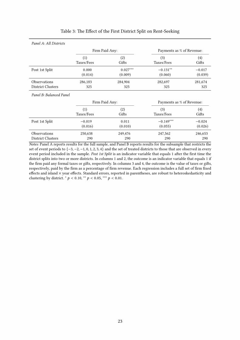
Table 3: �e E�ect of the First District Split on Rent-Seeking
Panel A: All Districts
Firm Paid Any: Payments as % of Revenue:
(1) (2) (3) (4)
Taxes/Fees Gi�s Taxes/Fees Gi�s
Post 1st Split 0.000 0.027∗∗∗ −0.131
∗∗ −0.017
(0.014) (0.009) (0.060) (0.039)
Observations 286,183 284,904 282,697 281,674
District Clusters 325 325 325 325
Panel B: Balanced Panel
Firm Paid Any: Payments as % of Revenue:
(1) (2) (3) (4)
Taxes/Fees Gi�s Taxes/Fees Gi�s
Post 1st Split −0.019 0.011 −0.149∗∗∗ −0.024
(0.016) (0.010) (0.055) (0.026)
Observations 250,638 249,476 247,562 246,653
District Clusters 290 290 290 290
Notes: Panel A reports results for the full sample, and Panel B reports results for the subsample that restricts the
set of event periods to {−3,−2,−1, 0, 1, 2, 3, 4} and the set of treated districts to those that are observed in every
event period included in the sample. Post 1st Split is an indicator variable that equals 1 a�er the �rst time the
district splits into two or more districts. In columns 1 and 2, the outcome is an indicator variable that equals 1 if
the �rm paid any formal taxes or gi�s, respectively. In columns 3 and 4, the outcome is the value of taxes or gi�s,
respectively, paid by the �rm as a percentage of �rm revenue. Each regression includes a full set of �rm �xed
e�ects and island × year e�ects. Standard errors, reported in parentheses, are robust to heteroskedasticity and
clustering by district.∗ p < 0.10,
∗∗ p < 0.05,∗∗∗ p < 0.01.
23
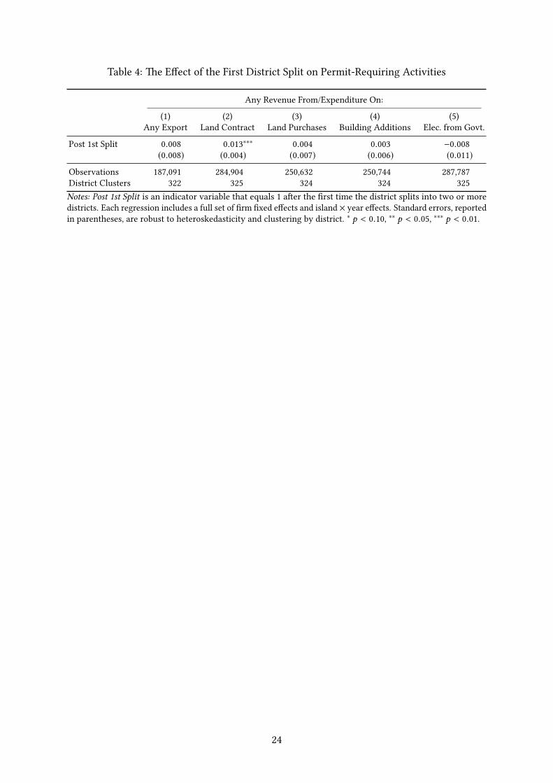
Table 4: �e E�ect of the First District Split on Permit-Requiring Activities
Any Revenue From/Expenditure On:
(1) (2) (3) (4) (5)
Any Export Land Contract Land Purchases Building Additions Elec. from Govt.
Post 1st Split 0.008 0.013∗∗∗
0.004 0.003 −0.008
(0.008) (0.004) (0.007) (0.006) (0.011)
Observations 187,091 284,904 250,632 250,744 287,787
District Clusters 322 325 324 324 325
Notes: Post 1st Split is an indicator variable that equals 1 a�er the �rst time the district splits into two or more
districts. Each regression includes a full set of �rm �xed e�ects and island × year e�ects. Standard errors, reported
in parentheses, are robust to heteroskedasticity and clustering by district.∗ p < 0.10,
∗∗ p < 0.05,∗∗∗ p < 0.01.
24
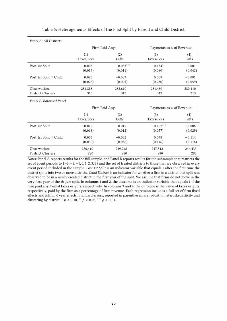
Table 5: Heterogeneous E�ects of the First Split by Parent and Child District
Panel A: All Districts
Firm Paid Any: Payments as % of Revenue:
(1) (2) (3) (4)
Taxes/Fees Gi�s Taxes/Fees Gi�s
Post 1st Split −0.003 0.033∗∗∗ −0.134
∗ −0.001
(0.017) (0.011) (0.080) (0.042)
Post 1st Split × Child 0.023 −0.033 0.009 −0.081
(0.026) (0.025) (0.230) (0.059)
Observations 284,888 283,610 281,430 280,410
District Clusters 313 313 313 313
Panel B: Balanced Panel
Firm Paid Any: Payments as % of Revenue:
(1) (2) (3) (4)
Taxes/Fees Gi�s Taxes/Fees Gi�s
Post 1st Split −0.019 0.015 −0.152∗∗∗ −0.006
(0.018) (0.012) (0.057) (0.029)
Post 1st Split × Child 0.006 −0.032 0.078 −0.114
(0.030) (0.036) (0.146) (0.116)
Observations 250,410 249,248 247,342 246,433
District Clusters 280 280 280 280
Notes: Panel A reports results for the full sample, and Panel B reports results for the subsample that restricts the
set of event periods to {−3,−2,−1, 0, 1, 2, 3, 4} and the set of treated districts to those that are observed in every
event period included in the sample. Post 1st Split is an indicator variable that equals 1 a�er the �rst time the
district splits into two or more districts. Child District is an indicator for whether a �rm in a district that split was
observed to be in a newly created district in the �rst year of the split. We assume that �rms do not move in the
very �rst year of the de jure split. In columns 1 and 2, the outcome is an indicator variable that equals 1 if the
�rm paid any formal taxes or gi�s, respectively. In columns 3 and 4, the outcome is the value of taxes or gi�s,
respectively, paid by the �rm as a percentage of �rm revenue. Each regression includes a full set of �rm �xed
e�ects and island × year e�ects. Standard errors, reported in parentheses, are robust to heteroskedasticity and
clustering by district.∗ p < 0.10,
∗∗ p < 0.05,∗∗∗ p < 0.01.
25
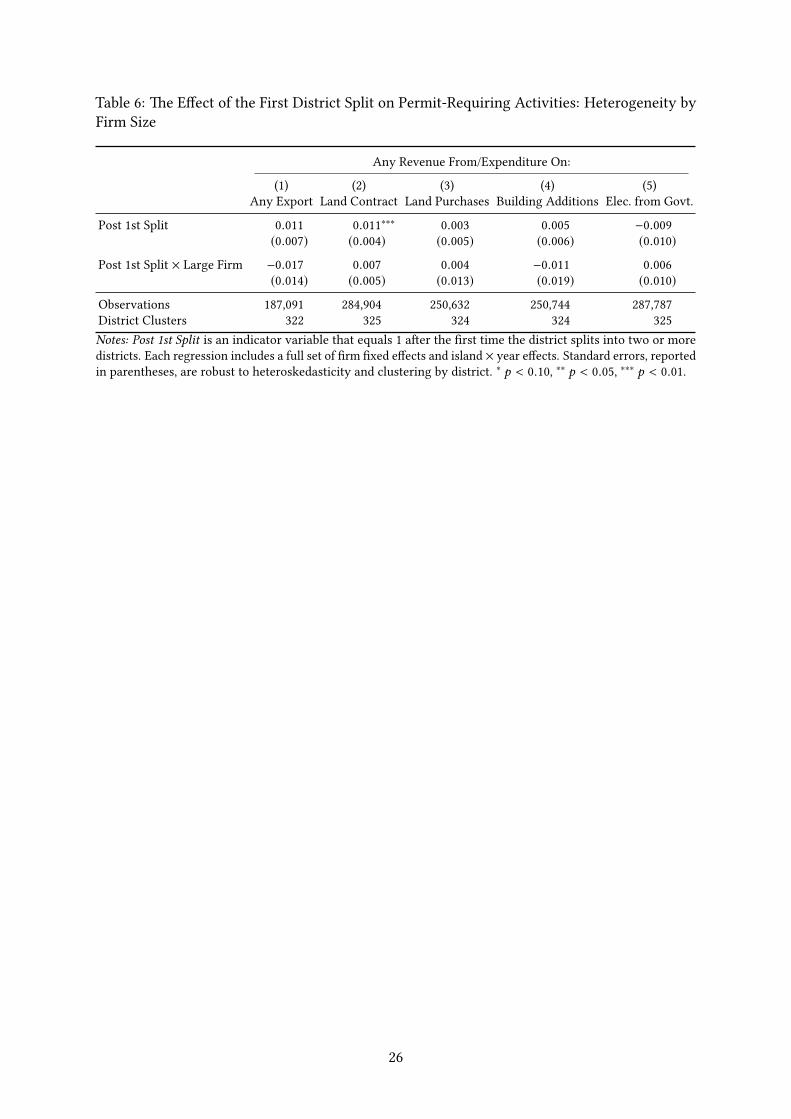
Table 6: �e E�ect of the First District Split on Permit-Requiring Activities: Heterogeneity by
Firm Size
Any Revenue From/Expenditure On:
(1) (2) (3) (4) (5)
Any Export Land Contract Land Purchases Building Additions Elec. from Govt.
Post 1st Split 0.011 0.011∗∗∗
0.003 0.005 −0.009
(0.007) (0.004) (0.005) (0.006) (0.010)
Post 1st Split × Large Firm −0.017 0.007 0.004 −0.011 0.006
(0.014) (0.005) (0.013) (0.019) (0.010)
Observations 187,091 284,904 250,632 250,744 287,787
District Clusters 322 325 324 324 325
Notes: Post 1st Split is an indicator variable that equals 1 a�er the �rst time the district splits into two or more
districts. Each regression includes a full set of �rm �xed e�ects and island × year e�ects. Standard errors, reported
in parentheses, are robust to heteroskedasticity and clustering by district.∗ p < 0.10,
∗∗ p < 0.05,∗∗∗ p < 0.01.
26
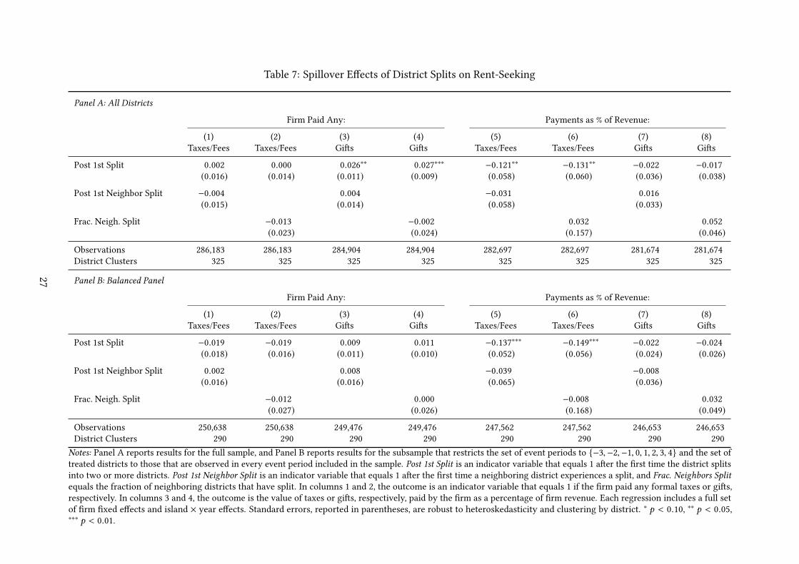
Table 7: Spillover E�ects of District Splits on Rent-Seeking
Panel A: All Districts
Firm Paid Any: Payments as % of Revenue:
(1) (2) (3) (4) (5) (6) (7) (8)
Taxes/Fees Taxes/Fees Gi�s Gi�s Taxes/Fees Taxes/Fees Gi�s Gi�s
Post 1st Split 0.002 0.000 0.026∗∗
0.027∗∗∗ −0.121
∗∗ −0.131∗∗ −0.022 −0.017
(0.016) (0.014) (0.011) (0.009) (0.058) (0.060) (0.036) (0.038)
Post 1st Neighbor Split −0.004 0.004 −0.031 0.016
(0.015) (0.014) (0.058) (0.033)
Frac. Neigh. Split −0.013 −0.002 0.032 0.052
(0.023) (0.024) (0.157) (0.046)
Observations 286,183 286,183 284,904 284,904 282,697 282,697 281,674 281,674
District Clusters 325 325 325 325 325 325 325 325
Panel B: Balanced Panel
Firm Paid Any: Payments as % of Revenue:
(1) (2) (3) (4) (5) (6) (7) (8)
Taxes/Fees Taxes/Fees Gi�s Gi�s Taxes/Fees Taxes/Fees Gi�s Gi�s
Post 1st Split −0.019 −0.019 0.009 0.011 −0.137∗∗∗ −0.149
∗∗∗ −0.022 −0.024
(0.018) (0.016) (0.011) (0.010) (0.052) (0.056) (0.024) (0.026)
Post 1st Neighbor Split 0.002 0.008 −0.039 −0.008
(0.016) (0.016) (0.065) (0.036)
Frac. Neigh. Split −0.012 0.000 −0.008 0.032
(0.027) (0.026) (0.168) (0.049)
Observations 250,638 250,638 249,476 249,476 247,562 247,562 246,653 246,653
District Clusters 290 290 290 290 290 290 290 290
Notes: Panel A reports results for the full sample, and Panel B reports results for the subsample that restricts the set of event periods to {−3,−2,−1, 0, 1, 2, 3, 4} and the set of
treated districts to those that are observed in every event period included in the sample. Post 1st Split is an indicator variable that equals 1 a�er the �rst time the district splits
into two or more districts. Post 1st Neighbor Split is an indicator variable that equals 1 a�er the �rst time a neighboring district experiences a split, and Frac. Neighbors Splitequals the fraction of neighboring districts that have split. In columns 1 and 2, the outcome is an indicator variable that equals 1 if the �rm paid any formal taxes or gi�s,
respectively. In columns 3 and 4, the outcome is the value of taxes or gi�s, respectively, paid by the �rm as a percentage of �rm revenue. Each regression includes a full set
of �rm �xed e�ects and island × year e�ects. Standard errors, reported in parentheses, are robust to heteroskedasticity and clustering by district.∗ p < 0.10,
∗∗ p < 0.05,
∗∗∗ p < 0.01.
27
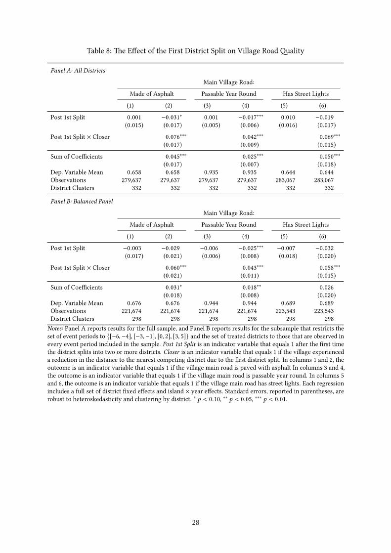
Table 8: �e E�ect of the First District Split on Village Road �ality
Panel A: All Districts
Main Village Road:
Made of Asphalt Passable Year Round Has Street Lights
(1) (2) (3) (4) (5) (6)
Post 1st Split 0.001 −0.031∗
0.001 −0.017∗∗∗
0.010 −0.019
(0.015) (0.017) (0.005) (0.006) (0.016) (0.017)
Post 1st Split × Closer 0.076∗∗∗
0.042∗∗∗
0.069∗∗∗
(0.017) (0.009) (0.015)
Sum of Coe�cients 0.045∗∗∗
0.025∗∗∗
0.050∗∗∗
(0.017) (0.007) (0.018)
Dep. Variable Mean 0.658 0.658 0.935 0.935 0.644 0.644
Observations 279,637 279,637 279,637 279,637 283,067 283,067
District Clusters 332 332 332 332 332 332
Panel B: Balanced Panel
Main Village Road:
Made of Asphalt Passable Year Round Has Street Lights
(1) (2) (3) (4) (5) (6)
Post 1st Split −0.003 −0.029 −0.006 −0.025∗∗∗ −0.007 −0.032
(0.017) (0.021) (0.006) (0.008) (0.018) (0.020)
Post 1st Split × Closer 0.060∗∗∗
0.043∗∗∗
0.058∗∗∗
(0.021) (0.011) (0.015)
Sum of Coe�cients 0.031∗
0.018∗∗
0.026
(0.018) (0.008) (0.020)
Dep. Variable Mean 0.676 0.676 0.944 0.944 0.689 0.689
Observations 221,674 221,674 221,674 221,674 223,543 223,543
District Clusters 298 298 298 298 298 298
Notes: Panel A reports results for the full sample, and Panel B reports results for the subsample that restricts the
set of event periods to {[−6,−4], [−3,−1], [0, 2], [3, 5]} and the set of treated districts to those that are observed in
every event period included in the sample. Post 1st Split is an indicator variable that equals 1 a�er the �rst time
the district splits into two or more districts. Closer is an indicator variable that equals 1 if the village experienced
a reduction in the distance to the nearest competing district due to the �rst district split. In columns 1 and 2, the
outcome is an indicator variable that equals 1 if the village main road is paved with asphalt In columns 3 and 4,
the outcome is an indicator variable that equals 1 if the village main road is passable year round. In columns 5
and 6, the outcome is an indicator variable that equals 1 if the village main road has street lights. Each regression
includes a full set of district �xed e�ects and island × year e�ects. Standard errors, reported in parentheses, are
robust to heteroskedasticity and clustering by district.∗ p < 0.10,
∗∗ p < 0.05,∗∗∗ p < 0.01.
28

9 Figures
Figure 1: �e Timing of De Jure and De Facto District Creation
(a) Two Moratoria Generated Idiosyncratic Variation in the Timing of De Jure District Creation
350
400
450
500
Num
ber o
f Dis
trict
s at
Sta
rt of
Yea
r
2000 2002 2004 2006 2008 2010 2012 2014Year
(b) Lag Time Between De Jure and De Facto District Creation
020
4060
80N
umbe
r of D
istri
cts
0 1 2 3Years Between First Legal Split and New District's Receipt of General Grant
Notes: Panel (a) plots the number of districts at the start of the year. �e two �at portions of the graph are due to
moratoria on district creation imposed by the central government during the periods 2004–2006 and 2009–2012.
Panel (b) shows the frequency distribution of the di�erence between the year of legal creation of the �rst new
district (within 2000 borders) and the year the new district �rst receives the general grant.
29
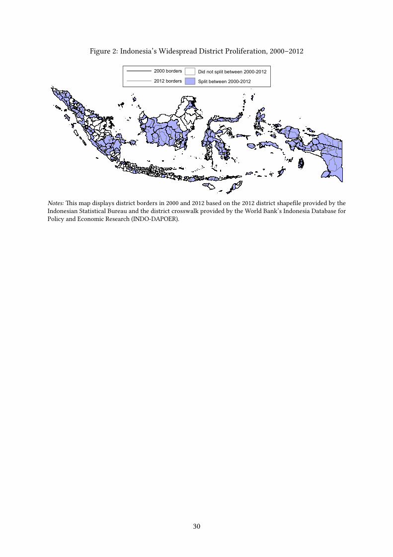
Figure 2: Indonesia’s Widespread District Proliferation, 2000–2012
2000 borders2012 borders
Did not split between 2000-2012Split between 2000-2012
Notes: �is map displays district borders in 2000 and 2012 based on the 2012 district shape�le provided by the
Indonesian Statistical Bureau and the district crosswalk provided by the World Bank’s Indonesia Database for
Policy and Economic Research (INDO-DAPOER).
30

Figure 3: �e E�ect of District Splits on Village Proximity to Competing Districts
Musi Banyuasin District, South Sumatra Province
Village bordersOriginal district bordersNew district borders
0 50 10025Kilometers
Notes: �is map displays the original district borders (thick solid lines) of Musi Banyausin prior to its (de jure) split
in 2002. �e thick dashed lines represent the new district borders following the split. �e child district, Banyuasin,
is located to the east of the new borders. �e example village, highlighted in orange, becomes signi�cantly closer
to a competing district as a result of the split. For many non-highlighted villages, the distance to the nearest
competing district does not change.
31

Figure 4: �e E�ect of the First District Split on Firm-Level Outcomes-0
.10
-0.0
50.
000.
050.
100.
15
-4+ -3 -2 -1 0 1 2 3 4 5 6+Years Since First Split
Firm Paid Any Formal Taxes or License Fees
-0.1
0-0
.05
0.00
0.05
0.10
0.15
-4+ -3 -2 -1 0 1 2 3 4 5 6+Years Since First Split
Firm Paid Any Gifts to Others
-0.5
0-0
.40
-0.3
0-0
.20
-0.1
00.
000.
100.
20
-4+ -3 -2 -1 0 1 2 3 4 5 6+Years Since First Split
Taxes/Fees as % of Revenue-0
.50
-0.4
0-0
.30
-0.2
0-0
.10
0.00
0.10
0.20
-4+ -3 -2 -1 0 1 2 3 4 5 6+Years Since First Split
Bribes as % of Revenue
Notes: �is �gure plots the estimates of {βs }s ∈S from (2) and their 95-percent con�dence intervals.
32
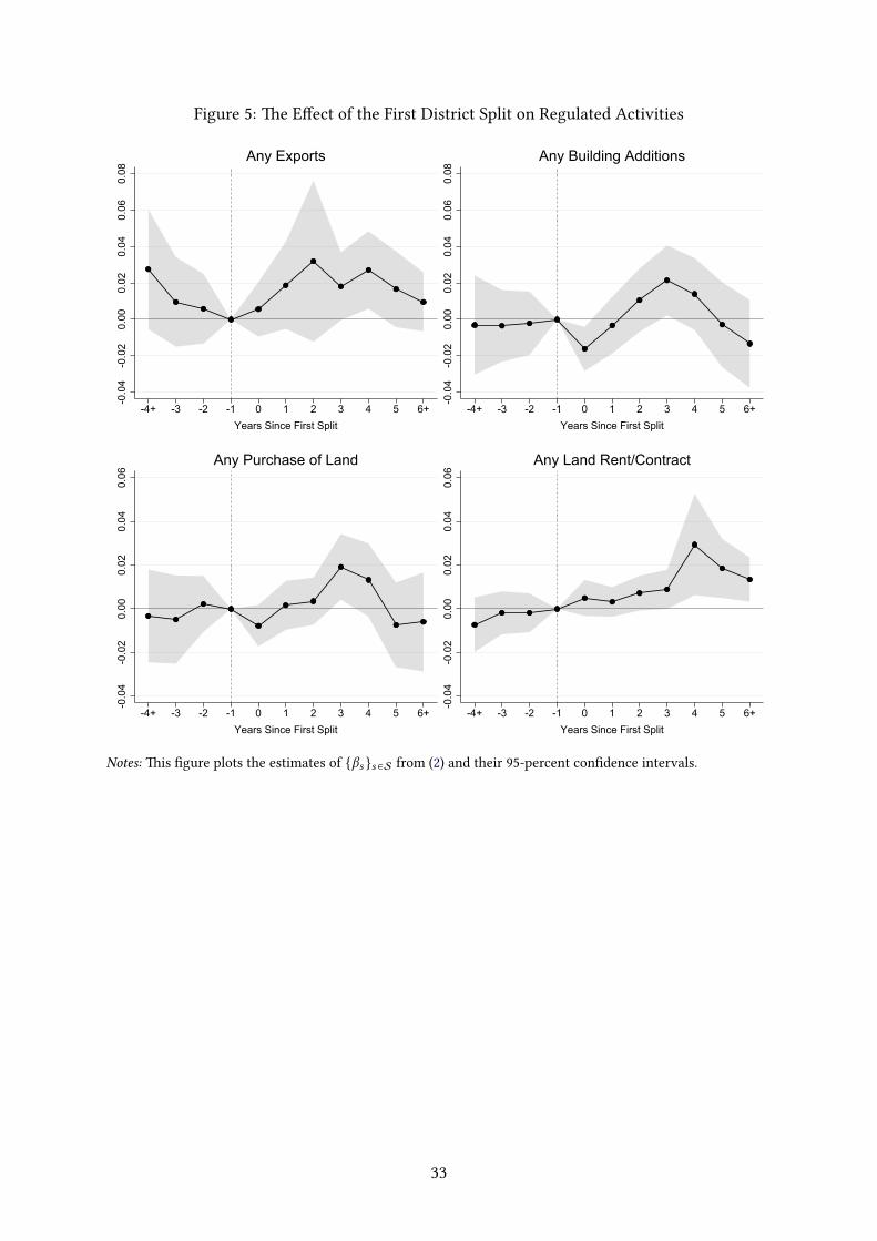
Figure 5: �e E�ect of the First District Split on Regulated Activities-0
.04
-0.0
20.
000.
020.
040.
060.
08
-4+ -3 -2 -1 0 1 2 3 4 5 6+Years Since First Split
Any Exports
-0.0
4-0
.02
0.00
0.02
0.04
0.06
0.08
-4+ -3 -2 -1 0 1 2 3 4 5 6+Years Since First Split
Any Building Additions
-0.0
4-0
.02
0.00
0.02
0.04
0.06
-4+ -3 -2 -1 0 1 2 3 4 5 6+Years Since First Split
Any Purchase of Land-0
.04
-0.0
20.
000.
020.
040.
06
-4+ -3 -2 -1 0 1 2 3 4 5 6+Years Since First Split
Any Land Rent/Contract
Notes: �is �gure plots the estimates of {βs }s ∈S from (2) and their 95-percent con�dence intervals.
33
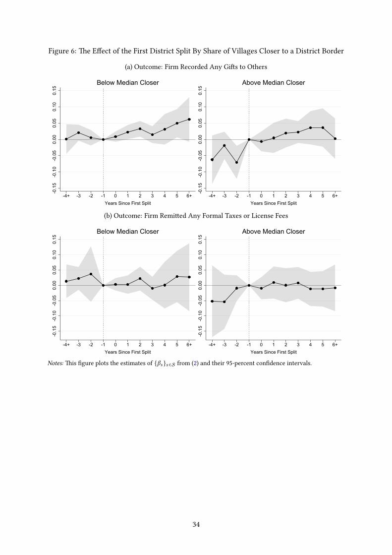
Figure 6: �e E�ect of the First District Split By Share of Villages Closer to a District Border
(a) Outcome: Firm Recorded Any Gi�s to Others
-0.1
5-0
.10
-0.0
50.
000.
050.
100.
15
-4+ -3 -2 -1 0 1 2 3 4 5 6+Years Since First Split
Below Median Closer
-0.1
5-0
.10
-0.0
50.
000.
050.
100.
15-4+ -3 -2 -1 0 1 2 3 4 5 6+
Years Since First Split
Above Median Closer
(b) Outcome: Firm Remi�ed Any Formal Taxes or License Fees
-0.1
5-0
.10
-0.0
50.
000.
050.
100.
15
-4+ -3 -2 -1 0 1 2 3 4 5 6+Years Since First Split
Below Median Closer
-0.1
5-0
.10
-0.0
50.
000.
050.
100.
15
-4+ -3 -2 -1 0 1 2 3 4 5 6+Years Since First Split
Above Median Closer
Notes: �is �gure plots the estimates of {βs }s ∈S from (2) and their 95-percent con�dence intervals.
34

Figure 7: �e E�ect of the First District Split By Whether Split Approved by Elected Mayor,
Balanced Panel
(a) Outcome: Firm Recorded Any Gi�s to Others
-0.1
0-0
.05
0.00
0.05
0.10
-1 0 1 2 3 4Years Since First Split
Pre Election
-0.1
0-0
.05
0.00
0.05
0.10
-1 0 1 2 3 4Years Since First Split
Post Election
(b) Outcome: Firm Remi�ed Any Formal Taxes or License Fees
-0.1
5-0
.10
-0.0
50.
000.
050.
10
-1 0 1 2 3 4Years Since First Split
Pre Election
-0.1
5-0
.10
-0.0
50.
000.
050.
10
-1 0 1 2 3 4Years Since First Split
Post Election
Notes: �is �gure plots the estimates of {βs }s ∈S from (2) and their 95-percent con�dence intervals.
35

Figure 8: Robustness of Firm-Level Results to Adding Controls
Baseline
Control for Ethnic Frac.
Control for Direct Elections
Control for General Grant
Control for All
Baseline
Control for Ethnic Frac.
Control for Direct Elections
Control for General Grant
Control for All
Firm Paid Any Taxes/Fees
Firm Paid Any Gifts
-0.02 0.00 0.02 0.04 0.06Coefficient on Post 1st Split
Baseline
Control for Ethnic Frac.
Control for Direct Elections
Control for General Grant
Control for All
Baseline
Control for Ethnic Frac.
Control for Direct Elections
Control for General Grant
Control for All
Taxes/Fees as % of Revenue
Gifts as % of Revenue
-0.30 -0.20 -0.10 0.00 0.10Coefficient on Post 1st Split
Notes: �is �gure plots the estimates of β from (1) and their 95-percent con�dence intervals a�er controlling for
various covariates. For each outcome, the �rst row reports the baseline estimate, the second row controls for
ethnic fractionalization, the third row controls for the presence of a directly elected mayor, the fourth row controls
for log General Grant revenue per capita and its square, and the ��h row controls for all of the aforementioned
covariates.
36

Figure 9: Average and Heterogeneous E�ects of the First District Split on Village Road �ality
(a) Outcome: Main Village Road Is Made of Asphalt-0
.10
-0.0
50.
000.
050.
10
-4+ -3 to -1 0-2 3-5 6+Years Since First Split
All Villages
Average Effect of First Split
-0.1
0-0
.05
0.00
0.05
0.10
-4+ -3 to -1 0-2 3-5 6+Years Since First Split
Became Closer No Change
Effects by Change in Proximity to Neighbor
(b) Outcome: Main Village Road Is Passable Year Round
-0.0
6-0
.04
-0.0
20.
000.
020.
040.
06
-4+ -3 to -1 0-2 3-5 6+Years Since First Split
All Villages
Average Effect of First Split
-0.0
6-0
.04
-0.0
20.
000.
020.
040.
06
-4+ -3 to -1 0-2 3-5 6+Years Since First Split
Became Closer No Change
Effects by Change in Proximity to Neighbor
(c) Outcome: Main Village Road Has Street Lights
-0.1
2-0
.08
-0.0
40.
000.
040.
080.
12
-4+ -3 to -1 0-2 3-5 6+Years Since First Split
All Villages
Average Effect of First Split
-0.1
2-0
.08
-0.0
40.
000.
040.
080.
12
-4+ -3 to -1 0-2 3-5 6+Years Since First Split
Became Closer No Change
Effects by Change in Proximity to Neighbor
Notes: �is �gure plots the estimates of {βs } in (4) (le�-hand side) and {βCs , βNs } in (5) (right-hand side), along
with their 95-percent con�dence intervals.
37

Figure 10: Robustness of Village Road �ality Results to Adding Controls
BaselineControl for Ethnic Frac.
Control for Direct ElectionsControl for General Grant
Control for All
BaselineControl for Ethnic Frac.
Control for Direct ElectionsControl for General Grant
Control for All
BaselineControl for Ethnic Frac.
Control for Direct ElectionsControl for General Grant
Control for All
Made of Asphalt
Passable Year Round
Has Street Lights
-0.05 0.00 0.05 0.10
Estimated Coefficient
Post 1st Split Post 1st Split × Closer
Notes: �is �gure plots the estimates of β and δ from (3) and their 95-percent con�dence intervals a�er controlling
for various covariates. For each outcome, the �rst row reports the baseline estimate, the second row controls for
ethnic fractionalization, the third row controls for the presence of a directly elected mayor, the fourth row controls
for log General Grant revenue per capita and its square, and the ��h row controls for all of the aforementioned
covariates.
38

A Additional Heterogeneity Analysis
A.1 Heterogeneity by Firm Size
Change below: interpretation of Bai et al is incorrect. In their model moving costs are increasingand concave in �rm size, which is determined by TFP. Concavity implies that when the �rm
grows, the bene�t of moving to another province with a lower bribe rate increases more than
the increase in moving costs. �is is because net-of-bribe pro�ts increase linearly in TFP.
Next we test whether the e�ect of district splits varies according to the size of the �rm. Bai
et al. (2019) �nd that when Vietnamese �rms grow larger, they pay less in bribes as a share
of �rm revenue. �ey claim that the result operates through intergovernmental competition,
arguing that larger �rms are more mobile and thus can more credibly threaten to leave the
jurisdiction. If �rm size is negatively correlated with mobility costs, we would also expect that
the fragmentation of districts would bene�t larger �rms more.
We do not �nd strong evidence of the impact of �rm size on district splits in this context.
Larger �rms are somewhat less likely to see an increase in bribes as a result of splits in their
original district and also less likely to see an increase in gi� payments as a share of total
revenue. Table B.1 displays the results from augmenting the baseline speci�cation with the
interaction term Post 1st Split × Large Firm, where Large Firm is an indicator variable that
equals 1 for �rms that recorded 200 or more employees at least once during the years prior to
the district’s �rst split. Now the coe�cient on Post 1st Split measures the e�ect of spli�ing on
small �rms, and the coe�cient on Post 1st Split × Firm Size measures how the e�ect of the �rst
split varies according to �rm size.
�e full-sample results in Panel A show that overall, consistent with the baseline results,
there is very li�e impact on either the intensive or extensive margin of tax payments. On the
other hand, there is a positive impact on gi� payments in the both the intensive and extensive
margin that is decreasing with �rm size. If we assume that the e�ect is linear as we do in this
speci�cation, the impact of splits only decreases the probability of gi� payments for very large
�rms. An increase in the number of employees at a �rm by 100 is associate with a decrease
in the e�ect of splits of gi� payments by 0.1 percentage points. However, the impact of �rm
size on the e�ect of district splits is not statistically signi�cant. Results in the sub sample of
districts that split around the moratorium are consistent with the full sample results. �e major
di�erence in this sub-sample is that the impact of the �rst split on the probability of any gi�
payments is negative in magnitude but not statistically signi�cant. Figures C.3 and C.4 show
that for all outcomes in both groups of large and small �rms, districts that split do not vary
systematically from those that do not or have not yet split, before splits.
39

A.2 Heterogeneity by Spatial Concentration of Industry
Firm size is only one indicator of moving costs for a �rm. Firms might rely on location-speci�c
resources that make it more di�cult for them to move in search of be�er local governance.
Rothenberg, Bazzi, Nataraj and Chari (2016) show that certain industries in Indonesia are
more spatially concentrated than others because they tend to rely on locally available inputs
such as natural resources and labor. �e more spatially concentrated an industry, the higher
the �rms’ moving costs and lower their bargaining power with district o�cials. We would
therefore expect that �rms in less spatially concentrated industries are more likely to bene�t
from district splits.
We examine how the impact of the district splits varies by industrial concentration of a
�rm’s industry prior to the split using the Ellison and Glaeser (1997) measure of industrial
concentration of industry j as
θj =Gj −
(1 −
∑d x
2
d
)Hj(
1 −∑
d x2
d
)(1 − Hj)
, (A.1)
where Hj =∑
f z2
fis the Her�ndahl index of concentration of employment across all establish-
ments f within industry j, and Gj =∑
d
(xd − sdj
)2
measures the sum of squared deviations
between sdj , the share of industry j’s national employment in district d , and xd , the share of
national employment in all industries in district d , where the district is de�ned according to
the boundaries in 2000. Our variable of interest is the average value of spatial concentration of
the �rm’s industry prior to the any district split where the �rm was located in 2000 or in the
earliest year they are observed in the data. Industry is identi�ed by 4-digit ISIC codes. Higher
values of θj indicate greater spatial concentration.
Table B.2 shows the results of interacting the post-split variable with this spatial concen-
tration measure. We see some weak evidence of heterogeneity by spatial concentration. �e
probability of any bribe payments is decreasing in spatial concentration, contrary to what we
would expect since �rms with high moving costs should have less bargaining power. However,
on the intensive-margin, bribe payments as a share of total revenue increase by more for �rms
in more spatially concentrated industries. Tax payments decrease following splits on both the
intensive and intensive margin and they fall by more for more spatially concentrated industries.
Results from only the districts that split around the moratorium are shown in panel B and are
very similar to results from the full sample.
Figures C.5 and C.6 show the results of the event-study speci�cation 2 split by a sample
of “low-concentration” �rms, which are �rms in industries with below-median spatial concen-
tration (i.e. less than 0.028), and a sample of above-median or “high-concetration” �rms. We
see that for all of our outcome variables of interest, �rms in these two groups exhibit parallel
trends prior to the �rst split.
40

B Appendix Tables
Table B.1: Heterogeneous E�ects of the First Split by Firm Size
Panel A: All Districts
Firm Paid Any: Payments as % of Revenue:
(1) (2) (3) (4)
Taxes/Fees Gi�s Taxes/Fees Gi�s
Post 1st Split 0.001 0.030∗∗∗ −0.127
∗∗ −0.024
(0.015) (0.009) (0.055) (0.039)
Post 1st Split × Firm Size −0.002 −0.011 −0.017 0.031∗∗∗
(0.003) (0.007) (0.076) (0.008)
Observations 286,183 284,904 282,697 281,674
District Clusters 325 325 325 325
Panel B: Balanced Panel
Firm Paid Any: Payments as % of Revenue:
(1) (2) (3) (4)
Taxes/Fees Gi�s Taxes/Fees Gi�s
Post 1st Split −0.018 0.013 −0.140∗∗∗ −0.031
(0.016) (0.010) (0.054) (0.026)
Post 1st Split × Firm Size −0.004 −0.007 −0.032 0.024∗∗∗
(0.004) (0.005) (0.104) (0.006)
Observations 250,638 249,476 247,562 246,653
District Clusters 290 290 290 290
Notes: Panel A reports results for the full sample, and Panel B reports results for the subsample that restricts
the set of event periods to {−3,−2,−1, 0, 1, 2, 3, 4} and the set of treated districts to those that are observed in
every event period included in the sample. Post 1st Split is an indicator variable that equals 1 a�er the �rst time
the district splits into two or more districts. Firm Size measured the maximum number of employees (in 1000s)
recorded for a �rm prior to the �rst split in their district. In columns 1 and 2, the outcome is an indicator variable
that equals 1 if the �rm paid any formal taxes or gi�s, respectively. In columns 3 and 4, the outcome is the
value of taxes or gi�s, respectively, paid by the �rm as a percentage of �rm revenue. Each regression includes
a full set of �rm �xed e�ects and island × year e�ects. Standard errors, reported in parentheses, are robust to
heteroskedasticity and clustering by district.∗ p < 0.10,
∗∗ p < 0.05,∗∗∗ p < 0.01.
41

Table B.2: Heterogeneous E�ects of the First Split by Industry Spatial Concentration
Panel A: All Districts
Firm Paid Any: Payments as % of Revenue:
(1) (2) (3) (4)
Taxes/Fees Gi�s Taxes/Fees Gi�s
Post 1st Split 0.002 0.033∗∗∗ −0.119
∗∗ −0.039
(0.019) (0.010) (0.059) (0.047)
Post 1st Split × Industry Spatial Concentration −0.240 −0.603 −1.418 2.490
(0.990) (0.574) (4.469) (2.129)
Observations 286,127 284,854 282,646 281,629
District Clusters 325 325 325 325
Panel B: Balanced Panel
Firm Paid Any: Payments as % of Revenue:
(1) (2) (3) (4)
Taxes/Fees Gi�s Taxes/Fees Gi�s
Post 1st Split −0.019 0.015 −0.069 −0.032
(0.019) (0.011) (0.061) (0.029)
Post 1st Split × Industry Spatial Concentration 0.005 −0.418 −7.641∗∗∗
0.800
(0.703) (0.525) (2.855) (1.917)
Observations 250,596 249,440 247,520 246,617
District Clusters 290 290 290 290
Notes: Panel A reports results for the full sample, and Panel B reports results for the subsample that restricts
the set of event periods to {−3,−2,−1, 0, 1, 2, 3, 4} and the set of treated districts to those that are observed in
every event period included in the sample. Post 1st Split is an indicator variable that equals 1 a�er the �rst
time the district splits into two or more districts. Concentration the value of the Ellison-Glaeser index of spatial
concentration as given in equation (A.1). Higher values of the index indicate greater spatial concentration. In
columns 1 and 2, the outcome is an indicator variable that equals 1 if the �rm paid any formal taxes or gi�s,
respectively. In columns 3 and 4, the outcome is the value of taxes or gi�s, respectively, paid by the �rm as a
percentage of �rm revenue. Each regression includes a full set of �rm �xed e�ects and island × year e�ects.
Standard errors, reported in parentheses, are robust to heteroskedasticity and clustering by district.∗ p < 0.10,
∗∗ p < 0.05,∗∗∗ p < 0.01.
42

Table B.3: �e E�ect of the First District Split on District Expenditure
Panel A: All Districts
Log Expenditure per Capita
(1) (2) (3) (4)
Total Infrastructure Personnel Administration
Post 1st Split 0.020 0.164∗∗ −0.050
∗0.175
∗∗∗
(0.026) (0.066) (0.025) (0.033)
Observations 4,381 3,754 4,411 3,791
District Clusters 336 336 336 336
Panel B: Balanced Panel
Log Expenditure per Capita
(1) (2) (3) (4)
Total Infrastructure Personnel Administration
Post 1st Split −0.018 0.206∗∗ −0.093
∗∗∗0.147
∗∗∗
(0.038) (0.088) (0.030) (0.037)
Observations 3,523 3,081 3,553 3,125
District Clusters 301 301 301 301
Notes: �e dependent variables are log district-level expenditure per capita in four expenditure categories: Total,Personnel, Administration, and Infrastructure. Post 1st Split is an indicator variable that equals 1 a�er the �rst time
the district splits into two or more districts. Each regression controls for the log of General Grant revenue per
capita and its square, and includes a full set of district �xed e�ects and island × year e�ects. Standard errors,
reported in parentheses, are robust to heteroskedasticity and clustering by district.∗ p < 0.10,
∗∗ p < 0.05,
∗∗∗ p < 0.01.
43

C Appendix Figures
Figure C.1: �e E�ect of the First District Split on Firm-Level Outcomes, Balanced Panel
-0.1
0-0
.05
0.00
0.05
0.10
-3 -2 -1 0 1 2 3 4Years Since First Split
Firm Paid Any Formal Taxes or License Fees
-0.1
0-0
.05
0.00
0.05
0.10
-3 -2 -1 0 1 2 3 4Years Since First Split
Firm Paid Any Gifts to Others
-0.5
0-0
.40
-0.3
0-0
.20
-0.1
00.
000.
10
-3 -2 -1 0 1 2 3 4Years Since First Split
Taxes/Fees as % of Revenue
-0.5
0-0
.40
-0.3
0-0
.20
-0.1
00.
000.
10
-3 -2 -1 0 1 2 3 4Years Since First Split
Bribes as % of Revenue
Notes: �is �gure plots the estimates of {βs }s ∈S from (2) and their 95-percent con�dence intervals.
44
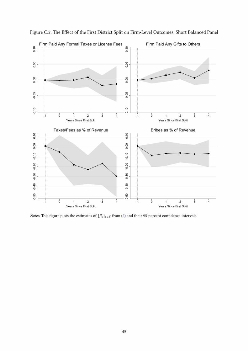
Figure C.2: �e E�ect of the First District Split on Firm-Level Outcomes, Short Balanced Panel-0
.10
-0.0
50.
000.
050.
10
-1 0 1 2 3 4Years Since First Split
Firm Paid Any Formal Taxes or License Fees
-0.1
0-0
.05
0.00
0.05
0.10
-1 0 1 2 3 4Years Since First Split
Firm Paid Any Gifts to Others
-0.5
0-0
.40
-0.3
0-0
.20
-0.1
00.
000.
10
-1 0 1 2 3 4Years Since First Split
Taxes/Fees as % of Revenue-0
.50
-0.4
0-0
.30
-0.2
0-0
.10
0.00
0.10
-1 0 1 2 3 4Years Since First Split
Bribes as % of Revenue
Notes: �is �gure plots the estimates of {βs }s ∈S from (2) and their 95-percent con�dence intervals.
45
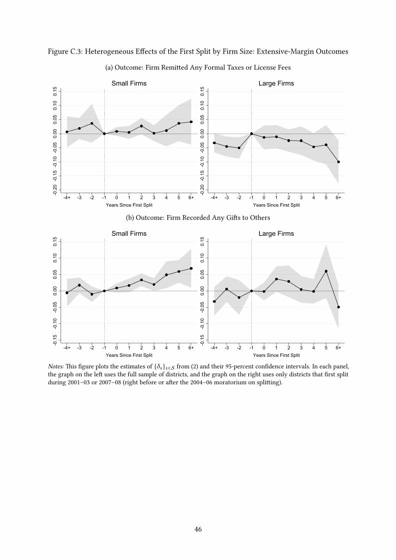
Figure C.3: Heterogeneous E�ects of the First Split by Firm Size: Extensive-Margin Outcomes
(a) Outcome: Firm Remi�ed Any Formal Taxes or License Fees
-0.2
0-0
.15
-0.1
0-0
.05
0.00
0.05
0.10
0.15
-4+ -3 -2 -1 0 1 2 3 4 5 6+Years Since First Split
Small Firms
-0.2
0-0
.15
-0.1
0-0
.05
0.00
0.05
0.10
0.15
-4+ -3 -2 -1 0 1 2 3 4 5 6+Years Since First Split
Large Firms
(b) Outcome: Firm Recorded Any Gi�s to Others
-0.1
5-0
.10
-0.0
50.
000.
050.
100.
15
-4+ -3 -2 -1 0 1 2 3 4 5 6+Years Since First Split
Small Firms
-0.1
5-0
.10
-0.0
50.
000.
050.
100.
15
-4+ -3 -2 -1 0 1 2 3 4 5 6+Years Since First Split
Large Firms
Notes: �is �gure plots the estimates of {δs }s ∈S from (2) and their 95-percent con�dence intervals. In each panel,
the graph on the le� uses the full sample of districts, and the graph on the right uses only districts that �rst split
during 2001–03 or 2007–08 (right before or a�er the 2004–06 moratorium on spli�ing).
46

Figure C.4: Heterogeneous E�ects of the First Split by Firm Size: Intensive-Margin Outcomes
(a) Outcome: Formal Taxes and License Fees as % of Revenue
-1.0
0-0
.50
0.00
0.50
-4+ -3 -2 -1 0 1 2 3 4 5 6+Years Since First Split
Small Firms
-1.0
0-0
.50
0.00
0.50
-4+ -3 -2 -1 0 1 2 3 4 5 6+Years Since First Split
Large Firms
(b) Outcome: Gi�s to Others as % of Revenue
-0.4
0-0
.20
0.00
0.20
0.40
-4+ -3 -2 -1 0 1 2 3 4 5 6+Years Since First Split
Small Firms
-0.4
0-0
.20
0.00
0.20
0.40
-4+ -3 -2 -1 0 1 2 3 4 5 6+Years Since First Split
Large Firms
Notes: �is �gure plots the estimates of {βs }s ∈S from (2) and their 95-percent con�dence intervals. In each panel,
the graph on the le� uses the full sample of districts, and the graph on the right uses only districts that �rst split
during 2001–03 or 2007–08 (right before or a�er the 2004–06 moratorium on spli�ing).
47

Figure C.5: Heterogeneous E�ects of the First Split by Industry Concentration: Extensive-
Margin Outcomes
(a) Outcome: Firm Remi�ed Any Formal Taxes or License Fees
-0.2
0-0
.15
-0.1
0-0
.05
0.00
0.05
0.10
0.15
-4+ -3 -2 -1 0 1 2 3 4 5 6+Years Since First Split
Low-Concentration Firms
-0.2
0-0
.15
-0.1
0-0
.05
0.00
0.05
0.10
0.15
-4+ -3 -2 -1 0 1 2 3 4 5 6+Years Since First Split
High-Concentration Firms
(b) Outcome: Firm Recorded Any Gi�s to Others
-0.3
0-0
.20
-0.1
00.
000.
100.
20
-4+ -3 -2 -1 0 1 2 3 4 5 6+Years Since First Split
Low-Concentration Firms
-0.3
0-0
.20
-0.1
00.
000.
100.
20
-4+ -3 -2 -1 0 1 2 3 4 5 6+Years Since First Split
High-Concentration Firms
Notes: �is �gure plots the estimates of {βs }s ∈S from (2) and their 95-percent con�dence intervals. In each panel,
the graph on the le� is for a sample of “low-concentration” �rms (i.e. �rms in industries with below-median
value of spatial concentration), and the graph on the right uses is for a sample of “high-concentration” �rms.
48
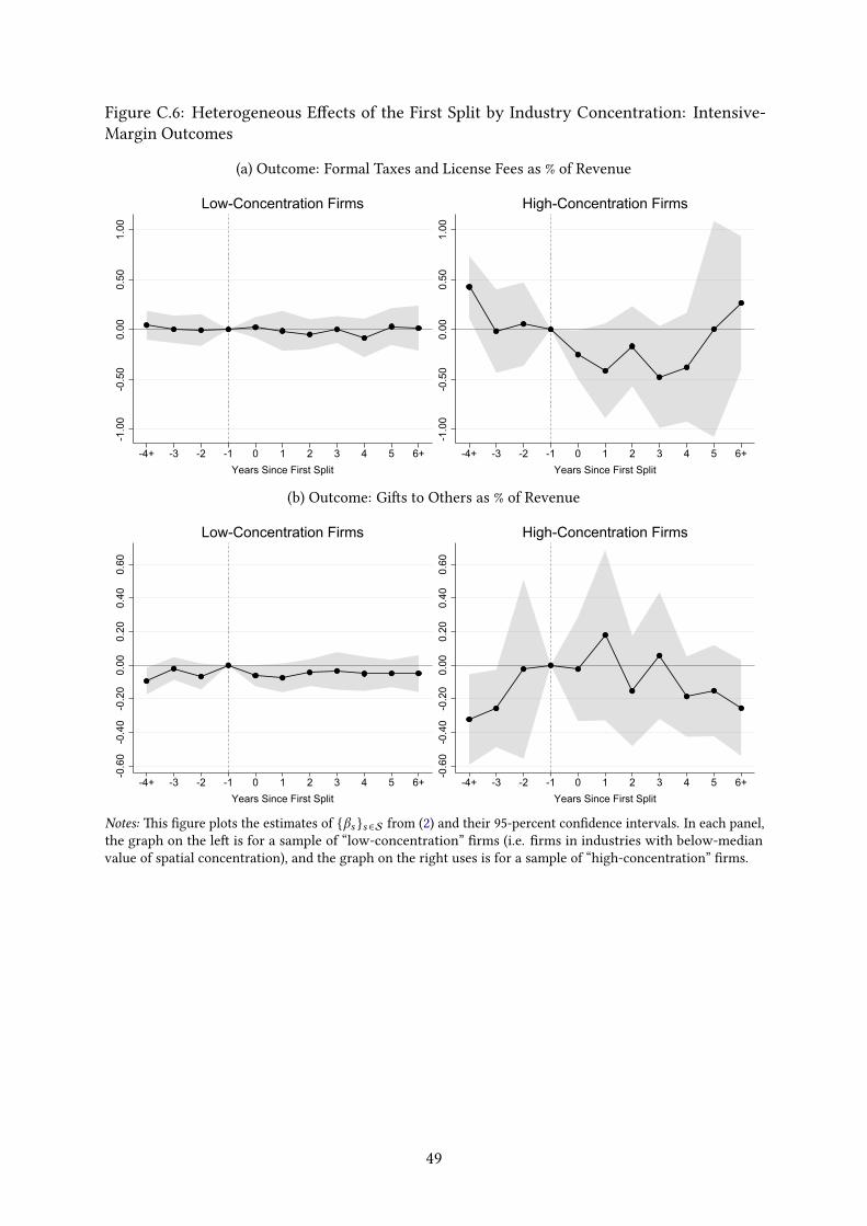
Figure C.6: Heterogeneous E�ects of the First Split by Industry Concentration: Intensive-
Margin Outcomes
(a) Outcome: Formal Taxes and License Fees as % of Revenue
-1.0
0-0
.50
0.00
0.50
1.00
-4+ -3 -2 -1 0 1 2 3 4 5 6+Years Since First Split
Low-Concentration Firms
-1.0
0-0
.50
0.00
0.50
1.00
-4+ -3 -2 -1 0 1 2 3 4 5 6+Years Since First Split
High-Concentration Firms
(b) Outcome: Gi�s to Others as % of Revenue
-0.6
0-0
.40
-0.2
00.
000.
200.
400.
60
-4+ -3 -2 -1 0 1 2 3 4 5 6+Years Since First Split
Low-Concentration Firms
-0.6
0-0
.40
-0.2
00.
000.
200.
400.
60
-4+ -3 -2 -1 0 1 2 3 4 5 6+Years Since First Split
High-Concentration Firms
Notes: �is �gure plots the estimates of {βs }s ∈S from (2) and their 95-percent con�dence intervals. In each panel,
the graph on the le� is for a sample of “low-concentration” �rms (i.e. �rms in industries with below-median
value of spatial concentration), and the graph on the right uses is for a sample of “high-concentration” �rms.
49


![IGC Issues: Bibliography€¦ · Intergovernmental Conference: Article 42 [of the TEU]: competition rules for agriculture products: memorandum by the United Kingdom (Circulated at](https://cdn.vdocuments.us/doc/165x107/60b1faaf19074a7e66165949/igc-issues-bibliography-intergovernmental-conference-article-42-of-the-teu.jpg)