
DISCUSSION PAPER SERIES
IZA DP No. 10501
Jacobus de HoopPatrick PremandFurio RosatiRenos Vakis
Women’s Economic Capacity and Children’s Human Capital Accumulation
JANUARY 2017

Any opinions expressed in this paper are those of the author(s) and not those of IZA. Research published in this series may include views on policy, but IZA takes no institutional policy positions. The IZA research network is committed to the IZA Guiding Principles of Research Integrity.The IZA Institute of Labor Economics is an independent economic research institute that conducts research in labor economics and offers evidence-based policy advice on labor market issues. Supported by the Deutsche Post Foundation, IZA runs the world’s largest network of economists, whose research aims to provide answers to the global labor market challenges of our time. Our key objective is to build bridges between academic research, policymakers and society.IZA Discussion Papers often represent preliminary work and are circulated to encourage discussion. Citation of such a paper should account for its provisional character. A revised version may be available directly from the author.
Schaumburg-Lippe-Straße 5–953113 Bonn, Germany
Phone: +49-228-3894-0Email: [email protected] www.iza.org
IZA – Institute of Labor Economics
DISCUSSION PAPER SERIES
IZA DP No. 10501
Women’s Economic Capacity and Children’s Human Capital Accumulation
JANUARY 2017
Jacobus de HoopUNICEF Office of Research, Innocenti
Patrick PremandThe World Bank
Furio RosatiILO, University of Rome Tor Vergata and IZA
Renos VakisThe World Bank

ABSTRACT
IZA DP No. 10501 JANUARY 2017
Women’s Economic Capacity and Children’s Human Capital Accumulation
Programs that increase the economic capacity of poor women can have cascading effects
on children’s participation in school and work that are theoretically undetermined. We
present a simple model to describe the possible channels through which these programs
may affect children’s activities. Based on a cluster-randomized trial, we examine how a
program providing capital and training to women in poor rural communities in Nicaragua
affected children. Children in beneficiary households are more likely to attend school one
year after the end of the intervention. An increase in women’s influence on household
decisions appears to contribute to the program’s beneficial effect on school attendance.
JEL Classification: D13, H43, I25, J22, J24, O15, O22, Q12
Keywords: women’s economic capacity, female empowerment, Nicaragua, child labor, human capital accumulation, field experiment
Corresponding author:Furio Camillo RosatiDepartment of Economics and FinanceUniversity of Rome Tor Vergatavia Columbia n. 200133 RomaItaly
E-mail: [email protected]
2
1. Introduction1
Investment in women’s economic capacity is often seen as an important tool not only
to achieve gender equality and address poverty, but also to improve children’s wellbeing
(e.g. World Bank, 2012). The rationale is that improvements in women’s economic
capacity are likely to be accompanied with increases in their access to financial resources
and in their intra-household bargaining power. Because women are presumed to have
stronger preferences for children’s wellbeing than men, their increased financial clout
and influence on household decisions is expected to translate into beneficial effects on
children. Indeed, as discussed in details in Duflo (2012), there is evidence that policies
that actively increase women’s access to resources and their influence on household
decisions can be advantageous for children.2 Although findings vary across studies, cash
1 This paper is based on a project initiated at the World Bank, and part of the research was carried out within UCW (Understanding Children's Work), a joint ILO, World Bank and UNICEF Programme. Funding was provided by the United States Department of Labour, the World Bank Gender Action Plan, and a BNPP trust fund. The views expressed here are those of the authors and should not be attributed to the ILO, the World Bank, UNICEF or any of these agencies’ member countries. This document does not necessarily reflect the views or policies of the United States Department of Labour, nor does mention of trade names, commercial products, or organizations imply endorsement by the United States Government.
A more detailed presentation of the program as well as its overall impacts beyond child labour and education is provided in the main report of the study (see Hatzimasoura, Premand and Vakis (2017)). The authors are grateful to Chrysanthi Hatzimasoura for her contributions to data analysis and to the main study report. The authors would like to thank Verónica Aguilera, Soledad Cubas, Amer Hasan, Karen Macours, Marco Manacorda, Enoe Moncada, Ana María Muñoz Boudet, Amber Peterman, Teresa Suazo and Egda Velez for contributions and advice at various points during the study design, its implementation, and analysis. The authors also thank participants in seminars at Bocconi University, UNICEF Office of Research – Innocenti, and Wageningen University. Finally, the authors would like to extend their gratitude to the team at Fundación Mujer y Desarrollo Económico Comunitario (FUMDEC) who implemented the intervention under the leadership of Rosa Adelina Barahona, Marlene Rodriguez and Milton Castillo.
2 Duflo (2012) indicates that the effects of these policies are not necessarily uniformly positive for children. Investments in children’s health and nutrition, for instance, may come at the expense of investments in children’s education.

3
transfers appear to have somewhat stronger beneficial effects on children’s health and
education when they are provided to women instead of men.3 Even in the absence of an
income transfer, household investment in children’s education appears to increase if the
bargaining power of women vis-à-vis their husband increases.4
Yet, evidence on the effects of interventions that aim to sustainably improve women’s
economic capacity is limited. Filling this knowledge gap is pressing given the popularity
of economic empowerment programs5 and because the effects of these programs on
children’s wellbeing are hard to predict and not necessarily favorable. From a theoretical
point of view, programs aimed at supporting women’s productive activities may change
children’s time allocation in complex ways. The economic activities of women may
increase household income and generate additional demand for children’s education and
leisure, thus reducing the supply of child labour. However, increased involvement of the
household in productive activities might raise the demand for child work, either directly
through children’s involvement in the household business or indirectly as children
substitute for their parents in domestic activities6. Finally, if the relative influence of
3 See, for instance, Benhassine et al. (2012), Duflo (2003), and Edmonds (2006) for direct comparisons of the effects of providing cash grants to women versus men. See Baird et al. (2014), Fiszbein and Schady (2009), Saavedra and Garcia (2012) for more general discussion of the effects of cash transfers on children’s education and de Hoop and Rosati (2014), Edmonds (2008), and Fiszbein and Schady (2009) for more general discussion of their effects on children’s work. 4 Rangel (2006), for instance, shows that investment in children’s education increased when Brazilian women’s bargaining power improved as a result of extended alimony rights. Reggio (2011) argues that, in Mexico, female children’s participation in work is negatively associated with women’s bargaining power. 5 Examples for multiple countries can be found in Banerjee et al. (2015), Cho and Honorati (2014), and McKenzie and Woodruff (2014). 6 Theoretically, additional capital provided to the household might be a gross substitute for children’s time in the production function and hence reduce the marginal productivity of child work. However, given the kind of economic activities and technologies typically supported by productive interventions for the poor, this possibility appears unlikely.

4
women on household decision making increases and women have stronger preferences
for children’s education than adult males, demand for children’s education might
increase. The final effects on children’s time allocation are, therefore, ambiguous and will
depend on the relative contributions of the three potential mechanisms.
This paper aims to shed more light on the relationship between programs fostering
women's productive capacity and children's activities. We begin by presenting a simple
model describing the channels through which productive programs targeting women
may affect children's participation in school and work. We then test the theoretical
predictions by analyzing the impact of a program that provided productive transfers (a
mix of cash and capital) to women in poor rural communities in Nicaragua. The program
offered households with at least one adult female member a package of benefits that
included (i) training on community organization and gender awareness, (ii) training in
technical or business skills to develop or expand small-scale household enterprises,
livestock or agricultural activities, (iii) capital transfers in the form of cash, seeds, or
livestock and (iv) follow-up technical assistance. The exact mix of capital transfers,
training and technical assistance was adjusted depending on the type of activity each
beneficiary wished to start or expand. We examine the impact of the program on child
labour and school attendance one year after the end of the intervention. Identification
stems from randomized program assignment among rural communities. Since
households in these communities were invited to apply before community
randomization, intent-to-treat program impacts can be estimated by comparing
outcomes in applicant households in treatment and control communities.7
7 The present paper is an output of a U.S. Department of Labor funding initiative,
which supported the collection and analysis of data on children’s productive activities as part of the experiment. The data collected for the project cover two domains of children’s outcomes: schooling and productive activities. Both of these domains are investigated in
5
Although the program did not directly aim to address children's participation in
school and work, one year after the end of the intervention we find that children in
beneficiary households are more likely to attend school, less likely to be working without
attending school, and less likely to be engaged in household chores. Based on the
theoretical framework, we explore the potential mechanisms explaining the observed
impacts. Consistent with its stated goals, the program led to changes in employment
patterns in beneficiary households. Beneficiary women in particular were more likely to
work in small-scale livestock and non-agricultural self-employment activities. Point
estimates for impact on earned income by women are positive, but not statistically
significant, and impact on overall household income is not statistically significant either.
Yet the program appeared to increase women's influence on household decision-making,
including in domains related to children’s outcomes. We suggest that the increase in
female influence on household decisions, possibly combined with the one-off increase in
household income resulting from the productive transfers, offset any potential increase
in the returns to children's work and contributes to explain the increase in school
attendance.
Our results are linked to the literature on the overall effectiveness of interventions
aimed at fostering productive employment and raising income-generating capacity
among the poor. The evidence, as discussed in several reviews, is mixed.8 Integrated
interventions addressing multiple constraints can be effective, particularly when the
this paper. Data collection did not comprise other data for children’s individual level outcomes. While analysis of child time use variables was not pre-registered, measurement of the effects of the program on children’s schooling and work is a stand-alone output of this research project. Hatzimasoura, Premand and Vakis (2017) provide a more extensive discussion of the effect of the program on households and adult women’s outcomes, the primary output of the overall study. 8 See, among others, Cho and Honorati (2014), McKenzie and Woodruff (2014), and Todd (2012).

6
interventions tackle capital constraints and are targeted to poor and vulnerable groups.9
There is less evidence of interventions providing skills training alone being effective,
particularly when targeted to existing micro-enterprise owners.10
Evidence on the impact of providing physical capital and skills training on children’s
time use is scarcer and results are varied. Banerjee et al. (2011), for instance, find limited
effects of the Indian THP (Targeting the Hardcore Poor) program on children’s school
attendance and labour supply. Bandiera et al. (2013) however, find that a similar
program in Bangladesh increased children's work in self-employment. Karlan and
Valdivia (2011) find that business training in Peru lowered children's participation in
work and increased their participation in school, although these effects are not
statistically significant.11
Del Carpio and Loayza (2012) study the effects of a conditional cash transfer program
complemented with a productive investment grant in Nicaragua. Their study focuses on
a different program than the one we analyze in this paper implemented in a different
(although not very dissimilar) region. The authors show that the intervention
contributed to reduce overall child participation in household chores and work, but
increased child participation in non-traditional activities related to commerce and retail.
This is consistent with the results of Del Carpio and Macours (2010) on the same
9 See for example Banerjee et al. (2015) for a multi-site study, Bandiera et al. (2013) for Bangladesh, Banerjee et al. (2011) for India, Blattman et al. (2014) for Uganda, or Macours et al. (2013) for Nicaragua. 10 See for instance Karlan and Valdivia (2011) for Peru and de Mel et al. (2012) for Sri Lanka. 11 Evidence on the effects of micro-credit programs, although conceptually somewhat different from the productive program we study, is more abundant. Various studies find increased work involvement among some specific groups of children (see Augsburg et al. (2012) for Bosnia and Herzegovina, Hazarika and Sarangi (2008) for Malawi, Islam and Choe (2013) for Bangladesh, and Nelson (2011) for Thailand). Yet, another study finds reductions in the probability that children are in work and not in school (Wydick (1999) for Guatemala).

7
conditional cash transfer program, who find that the productive investment grant added
to a cash transfer reinforced existing specialization in non-agricultural activities and
domestic work for girls, but that overall child labour did not increase.
The rest of the paper is organized as follows. Section 2 provides a theoretical
discussion of the effect of promoting women's productive capacity on children's
participation in school and work. Section 3 discusses the setting and presents the
program, study design and data. Section 4 discusses the strategy used to identify program
effects. Section 5 presents empirical results related to children's participation in school
and labour and discusses potential mechanisms. Section 6 concludes.
2. Theoretical framework
As discussed above, the effects of programs supporting productive activities of
women on children’s education and labour supply are theoretically undetermined. These
kinds of programs might increase the marginal productivity of child work if capital is a
gross complement of child work or if it induces adult labour supply shifts towards market
activities (which may increase the demand of children’s time for performing household
chores). Additional income generated through the program will tend to reduce child
labour involvement as long as leisure is a normal good. This might lead to an increase in
schooling or in children’s leisure time. The intervention will also lead to an increase in
school attendance as long as households are credit constrained and children’s school
attendance is suboptimal in the absence of the intervention. Finally, increases in
children’s schooling or reductions in child labour might also occur if (i) productive
programs increase adult women’s bargaining power within the households and (ii) these
same women have stronger preferences for investment in children's education than men.

8
To highlight these issues more formally, we consider a simplified version of an
overlapping generations model, in which adult household members value current
household consumption and children's future consumption. The latter is assumed to be
a function of household investment in education. Adult labour supply is inelastically fixed,
while parents decide about children’s time allocation between work and education12.
Household income is generated through the household production of marketable goods
or services, which is a function of the household supply of labour and of the stock of
capital.
In order to keep the exposition simple, we make several additional assumptions.
Households have three members: a mother, a father, and a child. These household
members can work only in the household activity and no hired labour is used in the
household production.13 More importantly, we assume that households cannot save or
borrow. To allow for savings will not alter the results, while the implications of non-
binding credit constraints will be discussed later. Finally, we only consider the
opportunity costs of children’s education. Allowing for direct costs will not change our
results.
More formally, the constraints faced by the households are the following. Children’s
time (normalized to 1) can be allocated to labour l or to education S:
(1) 𝑆 = 1 − 𝑙
12 For simplicity of exposition we do not consider that time can also be allocated to leisure. The implications of this assumption will be briefly discussed later. 13 As it will become apparent this assumption does not alter in any substantial way the results we are interested in.

9
Children's future consumption is assumed to be proportional to the amount of education
S received during childhood.
Current household consumption is given by the sum of exogenous income (y) and of
the value of the household production:
(2) 𝐶 = 𝑦 + 𝑔(𝑙𝑓 + 𝑙𝑚, 𝑙, 𝑘𝑓 + 𝑘𝑚)
where lf and lm, and kf and km respectively indicate the labour supplied by the adult female
and male member of the household and the capital stock (both physical and human)
owned by the female and male member of the household. We assume that male and
female labour and capital are perfect substitutes in the household's production, but that
they separately affect the relative power of the household member as discussed below.
We do not consider a unitary household, but assume instead that the two adult members
of the household have different utility functions, albeit both defined over the two goods
discussed above:
(3) 𝑈𝑓 = 𝑈𝑓 (𝐶, 𝑆) and 𝑈𝑚 = 𝑈𝑚 (𝐶, 𝑆)
where m and f indicate respectively the male and female household member.
There are different approaches to derive the demand functions for a non-unitary
household. We focus here on a cooperative Nash bargaining solution.14 Other approaches
are possible, like the Pareto efficient models suggested by Chiappori (1988), but in our
simple framework they will not lead to different results. We assume, therefore, that the
14 In the spirit of Manser and Brown (1980) and McElroy and Horney (1981).

10
demand functions of the household result from the maximization of the following
expression over the only decision variable l:
(4) 𝑀𝑎𝑥 [(𝑈𝑓 − 𝑈𝑓 ) (𝑈𝑚 − 𝑈𝑚
)]
where 𝑈𝑓 and 𝑈𝑚
indicate, respectively, the female and male fallback utilities, i.e. the
utility they would obtain if they would leave the household. We assume that the fallback
utilities depend on a set of characteristics X and on the ownership of productive capital
k:
(5) ��𝑖 = ��𝑖(𝑋𝑖, 𝑘𝑖) 𝑖 = 𝑓, 𝑚
The optimal level of children's labour supply, l*, is determined by:
(6) 𝑉 = ( 𝑈𝑓1′ 𝑔𝑙
′ − 𝑈𝑓2′ ) (𝑈𝑚 − 𝑈𝑚
) + ( 𝑈𝑚1′ 𝑔𝑙
′ − 𝑈𝑚2′ ) (𝑈𝑓 − 𝑈𝑓
) = 0
where the apex refers to the order of differentiation and the numerical subscript to the
argument of the function.
As is evident from (6), l* is determined as a weighted average of the levels of child
labour supply optimal, respectively, for the mother and the father. The weights are given
by their “relative” power. If we assume that women have a stronger preference than men
for the education of children (and their future welfare) then in equilibrium ( 𝑈𝑓1′ 𝑔𝑙
′ −
𝑈𝑓2′ ) < 0 and ( 𝑈𝑚1
′ 𝑔𝑙′ − 𝑈𝑚2
′ ) > 0. In other words, the equilibrium child labour supply

11
will be lower than that preferred by men and higher than that preferred by women
should they have been able to decide by themselves.
In this setup, a program aiming to provide women with additional capital and to
empower them, can be analyzed by looking at the impact of a marginal increase in kf. By
totally differentiating (6) we obtain:
(7) 𝑑𝑙∗
𝑑𝑘𝑓 = −
𝜕 𝑉
𝜕 𝑘𝑓
𝜕𝑉
𝜕 𝑙∗
as the denominator of the right hand side of (7) is negative by second order conditions,
𝑠𝑖𝑔𝑛 𝑑𝑙∗
𝑑𝑘𝑓= 𝑠𝑖𝑔𝑛
𝜕 𝑉
𝜕 𝑘𝑓 and
(8) 𝜕 𝑉
𝜕 𝑘𝑓= ( 𝑈𝑓1
′′ 𝑔𝑙′ 𝑔𝑘
′ + 𝑈𝑓1′ 𝑔𝑙𝑘
′ ) (𝑈𝑚 − 𝑈𝑚 ) + ( 𝑈𝑚1
′′ 𝑔𝑙′ 𝑔𝑘
′ +
𝑈𝑚1′ 𝑔𝑙𝑘
′ ) (𝑈𝑓 − 𝑈𝑓 ) − 𝑈𝑓𝑘
( 𝑈𝑚1′ 𝑔𝑙
′ − 𝑈𝑚2′ )
Equation (8) allows us to identify three effects of a change of k on education and the
supply of child labour. Overall the sign of (8) is undetermined, as it is the result of
contrasting effects. The increased availability of capital can affect the productivity of child
labour, as shown by the terms in 𝑈𝑓1′ 𝑔𝑙𝑘
′ and 𝑈𝑚1′ 𝑔𝑙𝑘
′ . In particular, if capital and child
labour are gross complements, 𝑔𝑙𝑘′ > 0, the supply of child labour will tend to increase
(and children's participation in school will decrease) as a result of the increased
availability of capital. The opposite will happen if capital is a substitute for child labour.
There is a positive income effect on education (negative income effect on work) given
by the terms 𝑈𝑓1′′ 𝑔𝑙
′ 𝑔𝑘′ and 𝑈𝑚1
′′ 𝑔𝑙′ 𝑔𝑘
′ . If credit markets were perfect, investment in

12
education and consumption decisions would be separable and the income effect would
disappear. If, on the other hand, leisure were also valued in the utility function and it were
a normal good, then a negative income effect can be present also if capital markets are
perfect.
Finally, if the fallback utility of women is positively affected by their increased
ownership of capital, 𝑈𝑓𝑘 > 0, and women value children’s education more than men,
𝑈𝑚1′ 𝑔𝑙
′ − 𝑈𝑚2′ > 0, women's increased bargaining power through the provision of capital
will tend to increase consumption of education and reduce children's labour supply.
3. Empirical study design and data
3.1 Nicaraguan Country Context
Nicaragua is classified by the World Bank as a lower middle income country. In 2010
it had a GDP per capita of about US$153515. In the same year, about 49% of women aged
15 to 64 were economically active, compared to about 82% of men. Nearly 60% of the
women who were economically active were self-employed.
School participation is not yet universal among Nicaragua's children. While the
country's 2010 net primary school enrollment rate was 92%, it is estimated that only
about half of the children who entered primary school would reach the final grade.16
15 The figures in the remainder of this section, with the exception of those related to children's economic activities, are drawn from the World Bank's development indicators database: http://data.worldbank.org/country/nicaragua. After correcting for purchasing power parity, the GDP per capita translates to about US$3962. 16 Latest figure is for 2007.

13
Concomitantly, the net secondary school enrollment rate was only about 45%. Literacy
rates are about 78% in the adult population (15+) and about 87% among youths (15 to
24).17
It is common for children to be involved in economic activities, even if they have not
yet reached the minimum legal working age of 14.18 Based on the 2010 Encuesta Continua
de Hogares, the Understanding Children's Work programme estimates that nearly 37%
of children aged 13 are economically active.19 About 78% of these children combine work
and school. Boys are more likely to work than girls (48% vs. 26%). Rates of participation
in economic activities are higher in rural areas (49%) than in urban areas (25%). Boys
who are economically active mostly work in agriculture (71%) although it is also
common form them to be active in commerce (14%). Girls who are economically active
are slightly more likely to work in commerce (35%) than in agriculture (32%).
3.2 The Program
In 2009/10, a Nicaraguan NGO (Fundación Mujer y Desarrollo Comunitario, or
FUMDEC)20, implemented a productive transfer program with support from the World
Bank21. The intervention built on a model in place in other communities in northern
Nicaragua since 1996, and had two main objectives: (i) to facilitate income generation
and diversification by promoting women’s economic activities, and (ii) to foster gender
17 Latest figure is for 2005. 18 For more information on legislation, we refer to the website of the US Department of Labour: http://www.dol.gov/ilab/reports/child-labour/nicaragua.htm 19 http://ucw-project.org/Pages/Tables.aspx?id=1602 20 For more information about FUMDEC, see http://fumdec.org. 21 See Hatzimasoura, Premand and Vakis (2017) for a more detailed description of the program as well as its overall impacts beyond education and child labour.

14
empowerment by improving women’s aspirations, their participation in households’
economic decisions as well as their social participation.
To achieve these objectives, the program offered households with at least one female
member 16 to 60 years old a package of benefits that included (i) training on community
organization and gender awareness, (ii) training in technical or business skills to develop
or expand small-scale household enterprises, livestock or agricultural activities of their
choice, (iii) capital transfers in the form of cash, seeds, or livestock and (iv) follow-up
technical assistance. The exact mix of capital transfers, training and technical assistance
was adjusted depending on the type of activity that each beneficiary wished to start or
expand: non-agricultural household enterprises, livestock, or other small-scale
agricultural activities.
The program included three main phases. First, beneficiaries were offered various
training workshops on community organization and gender awareness.22 The
community organization training included 4 modules for all beneficiaries on how to form
and organize women’s groups, as well as two additional modules for selected leaders on
managing women’s groups. The gender awareness training was offered to all
beneficiaries and included 8 modules on issues such as gender identity, self-esteem,
reproductive health, violence, and laws that protect women. These trainings were
delivered in the community. In addition, a gender awareness training targeted a small
number of selected men, usually leaders’ spouse, who were trained together in a central
location on a sub-set of the aforementioned themes. Second, beneficiaries were offered
training in technical or business skills to develop or expand small-scale household
enterprises, livestock or agricultural activities of their choice. Each beneficiary was
22 The next section describes the beneficiary selection process

15
offered between 4 and 6 training sessions. The scope of the training depended on the
activity chosen by individuals. It focused on technical skills and crop management for
individuals who chose agricultural activities. It tackled livestock management and related
technical skills for individuals who chose livestock activities. And it covered basic
business skills for individuals who chose small business activities. Third beneficiaries
received capital transfers in the form of cash, seeds, or livestock. After the transfers,
follow-up technical assistance visits were organized.23
The package had an average value of US$602 per beneficiary (the exact value
depending on the type of activity being supported).24 It included US$316 in direct capital
transfers (in the form of a mix of cash, seeds and livestock) and US$286 that covered the
costs of training and technical assistance. More than 80 percent of the targeted
households were estimated to live on average with less than US$2 per capita per day, and
the package amounted to around 24% of pre-transfer annual household consumption, a
rather sizeable magnitude.
3.3 Beneficiary Selection, Study Design and Data
The program operated in Santa Maria de Pantasma, one of Nicaragua’s poorest
municipalities. For the purpose of evaluating the program, a group of 24 communities
was identified25. Baseline data were collected in June and July 2009, before households
23 One additional component of the program, not yet implemented at the time of the follow-up survey, consisted of the creation of community banks. For this purpose, the program would provide training in management and organization to community leaders and initial technical support. It was envisioned that these banks would eventually become as a sustainable source of credit for the community. 24 In addition, administrative costs for the pilot amounted to US$225 per beneficiary, for a ratio of administrative costs to total transfers of 37%. 25 The 24 communities were selected on the basis of 5 criteria (i) they had to be located in a rural area, (ii) they should not have benefitted from related interventions, (iii) they needed to contain a minimum of 20 households, (iv) they needed to be located in an area

16
were informed about the program and invited to enroll. Baseline data is available for the
universe of eligible applicant and non-applicant households in the 24 communities.
Baseline information includes household and dwelling characteristics, household
composition and a number of household and individual socio-economic characteristics.
For individuals aged 6 years or more, the baseline survey collected information on
completed education, school enrollment, school attendance and involvement in economic
activities in the week preceding the survey.
Following the completion of the baseline survey, households in all eligible
communities were informed about the program and invited to enroll (apply) during a
series of community meetings held in July and August 2009. Specifically, all the potential
beneficiaries identified in the baseline survey were invited to an information assembly
organized by the implementing NGO. The invitation process was undertaken in
collaboration with community leaders and included door-to-door invitations of each
household. A total of 78% of invited individuals participated in the first assembly. During
that assembly, the program objectives and components were presented, and households
were informed that participation in the program was conditional on their community
being selected. All potential beneficiaries were asked to consider signing up for the
program. Approximately a week after the first assembly, a second assembly was held and
potential beneficiaries were asked to signal whether they were interested to enroll
(conditional on their community being selected). Out of all households in the target
communities, 45% enrolled, 50% did not enroll and 5% were not eligible as they did not
have a female member between the ages of 16 and 60.
that was well-known to the local NGO, and (v) the local authorities had to agree with the (potential) implementation of the program in their community.

17
Hatzimasoura, Premand and Vakis (2017) analyze the profile of households who self-
selected into the program. They show that program applicants tend to be better-off in
terms of education and assets, as well as more likely to be engaged in self-employment
activities. Women who self-select into the program also participate more in intra-household
decision-making. These patterns are consistent with the experience of the implementing NGO
in communities where they had been operating for several years, which suggests that better-
off and more empowered women are more likely to come forward and enroll in the program
initially, while relatively poorer and less empowered women eventually join later after the
program is more established in the community.26
In the context of this paper, since we know who the interested applicants in both the
treatment and comparison groups are, the selection pattern does not affect the internal
validity of the results. Indeed, as households were asked to enroll prior to community
randomization, applicant households (and potential beneficiaries within these
households) are known in both treatment and control communities. As such, intent-to-
treat program effects can be estimated based on counterfactual outcomes among
applicants in the control communities. In terms of external validity, the results of the study
should be interpreted as applying to a population of slightly better-off and more empowered
women in remote rural communities where nearly everyone is poor.
After individuals enrolled in the program, a public lottery was organized in the
municipal headquarters to allocate the communities to the treatment and control groups.
Communal and municipal leaders were invited along with representatives from each
community, from the local NGO and the World Bank. Selection of communities was based
on block randomization within (10) groups of neighboring communities (2 or 3
26 In the context of the study, enrolment was closed after the initial enrolment period, and there was no new intake of beneficiaries until after the follow-up survey.

18
depending on the block). The lottery led to the selection of 13 treatment and 11 control
communities, containing respectively 405 and 472 eligible households that did apply to
the program, 417 and 563 eligible households that did not apply, and 41 and 58 ineligible
households (i.e. households without a female member aged 16 to 60). The intervention
was implemented between September 2009 and August 2010. By August 2010, the
training modules were fully implemented and all the capital transfers were completed.
A follow-up survey was administered from June to August 2011 to all the households
that had been interviewed at baseline and could be tracked. Tracking was conducted at
the household level and households who left the experimental communities or household
members who left the household were not followed, although the survey collects
information on households who migrated to other experimental communities and on
individuals joining existing households.27 The follow-up survey was more extensive than
the baseline survey. In addition to the questions from the baseline survey, it also collected
information on a wider range of outcomes including involvement in economic activities
in the 12 months prior to the interview.
4. Empirical strategy
4.1 Schooling and child labour outcomes
In the analysis, we focus primarily on the effect of the program on school attendance
in the current school year and participation in work in the 12 months prior to the
interview. School attendance was measured both in the baseline and follow-up surveys.28
27 Although we have information on individuals who moved into the households (and were not observed at baseline), we leave these individuals out of the analysis. 28 We consider individuals to be attending school if the answer to the question “is … attending school this school year?” is “yes”.

19
As the baseline and follow-up questionnaire were administered in the middle of the
school year, which runs from February to November, seasonal effects should not be a
source of concern. In addition to school attendance over the school year, we also examine
regular school attendance over the last month prior to the survey (i.e. school attendance
without absence from school in the past 30 days for any reason other than: illness,
holiday, teacher not present or on strike)
We define individuals as working if they participated in any economic activity on own
account or as wage workers in the 12 months prior to the interview. This information on
employment over the last year was collected only as part of the follow-up survey. We
separately examine three kinds of work: agricultural activities, livestock and non-
agricultural activities for own account and wage work.29 We classify children as engaged
in household chores if they engaged in any of the following activities in the week prior to
the interview: collecting firewood, collecting water, and other household activities such
as washing clothes, caring for siblings, cooking, or cleaning. This information was
collected for children aged 6 to 16 as part of the follow-up survey.
To the extent possible, we also examine variations in the intensive margin of work
and household chores. For children aged 6 to 16, the follow-up survey asked about usual
weekly hours during the school year in up to three main economic activities and we sum
the hours worked to measure “total hours worked”. Similarly, we sum hours in the three
categories of household chores in the week prior to the interview to measure “total hours
in household chores”.
29 The non-agricultural activities on own account include household production, commerce, manufacturing, or services. Wage employment covers both agricultural wage work and non-agricultural wage jobs.

20
In order to probe the robustness of the main results, we exploit the information on
work in the week prior to the interview, which is available both at baseline and follow-
up.30
4.2 Sample and attrition
As we study the impact of the productive transfer program on children’s work and
school participation, we restrict our sample to (households with) children aged 6 to 15
at baseline (8 to 17 at follow-up). This gives a sample of 647 households that applied to
participate in the program, with 1923 adults and 1458 children in the relevant age range.
Over 95% of these households were observed at follow-up. Because individuals were not
tracked if they had left the household, the probability that individuals are observed at
follow-up is somewhat lower: about 87% for adults and about 91% for children.
Appendix table 1 examines whether attrition at follow-up is significantly different in
households residing in treatment and control communities at baseline. It reports OLS
regressions of the indicator for being interviewed at follow-up on the indicator for living
in a treatment village at baseline. Standard errors are clustered at the village level. Since
the number of clusters is small (24), we are likely to over-reject the null-hypothesis that
the program has no effect. Following Burde and Linde (2013), we therefore calculate
statistical significance relative to the small-sample t-distribution with 23 degrees of
freedom.
30 We rely on two questions. The first is whether individuals worked in the week prior to the interview. The second, asked only to individuals who initially respond that they did not work in the week prior to the interview, is whether they participated in any of the following economic activities: (i) sale of goods, (ii) washing, ironing, or sewing for others, (iii) preparing and selling bread, tortillas, sweets, crafts and other items, (iv) work as an apprentice, (v) agricultural work (cultivation or caring for livestock), (vi) tourism, (vii) fishery, or (viii) other economic activities (not further defined). We classify individuals as working if they answer “yes” either to the first or the second question.

21
Regression results indicate that the attrition rate of applicant households and
children was marginally lower in treatment than in control communities. However, when
we include baseline covariates (discussed in more details below) as controls in the
regressions, estimates become smaller and not statistically significant, suggesting that
controlling for baseline characteristics limits potential bias due to differential attrition.
4.3 Descriptive statistics and estimation strategy
Table 1 displays the mean values of a set of household level31 baseline covariates in
the control communities (column (1)): literacy and gender of the household head, an
asset index,32 a dummy for whether any land is owned by the household, bedrooms per
capita, distance to the closest school and to the closest health center, distance to schools
and health centers, household size, share of male adults in the household, share of adults
in ten-year age groups, dwelling characteristics, and women’s influence on household
decisions related to children. The table illustrates the high level of deprivation in the
study region. Nearly 40% of household heads are illiterate. About 10% of households live
in a wooden or improvised dwelling and, although nearly 90% of the households own
their dwelling, only about 45% have a property title. The main material of the dwelling’s
floor is typically dirt and walls are rarely made of brick or concrete. Over 50% of
households rely on rivers for water and nearly 50% of households have no sanitary
facilities in the home. Only about 1 in 10 households is connected to the electricity grid.
31 All figures reported in this subsection are for households and individuals that were observed also at follow-up. 32 This is computed as the first principal component of 13 assets: radio recorder, kitchen, vehicle, refrigerator, fan, grinding machine, iron, TV, bicycle, eating utensils (plates, glasses, and cutlery), kitchen utensils, table, and chairs.

22
Results related to women’s influence on household decisions are based on a survey
module asking (potential) female beneficiaries of the program “who has the last word
on…?” a list of household decisions, including: children’s school participation,
expenditures on children’s clothing, and taking children to a health center in case of
illness. The following four answer categories were provided: the beneficiary herself, her
spouse, together, and another person. About 73% of women have a say in decisions
regarding children’s school attendance (either individually or jointly with their spouse),
56% in decisions related to the purchase of children’s clothes, and the large majority
(91%) in decisions related to children’s visits to health centers.
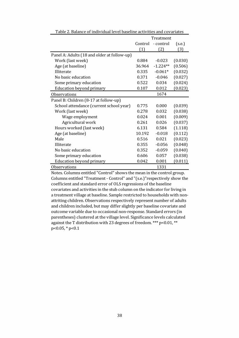
Table 2 shows the mean values of the outcome variables and of individual covariates
for adults and children who lived in control communities at baseline. Nearly 90% of the
adults worked in the week prior to the interview. Men are markedly more likely to work
(98% of the men in the control group is economically active) than women (79%).33 28%
of children from applicant households are engaged in some type of work, mostly in
agriculture, during the week prior to the interview and 78% of children attended school.
We test the success of the randomization by regressing selected baseline
characteristics on the treatment dummy among households and individuals observed at
follow-up. Tables 1 and 2 report the coefficients on the treatment dummy (column (2))
together with the clustered standard errors (column (3)). By and large, baseline
characteristics are not significantly correlated with the treatment dummy. We observe
statistically significant imbalances in the following baseline characteristics: household
composition (female household head and percentage of older adults), distance to school,
33 Results not displayed.

23
roof materials, and women’s influence on decisions related to children’s health care visits.
As we explain below, we correct for these imbalances in our estimates.
Our primary outcome variables, children’s schooling and work, were balanced at
baseline. Coupled with the observation that attrition did not differentially affect the
composition of the treatment and control groups (and more so when we include
additional baseline controls), it gives us reasonable confidence in the internal validity of
the experiment.34
We rely on randomized assignment to identify the program’s impact by employing a
simple reduced form model. Formally, we estimate cross-section regressions as follows:
(9) 𝑌𝑖𝑐1 = 𝛽0 + 𝛽1𝑇𝑅𝐸𝐴𝑇𝑐1 + 𝛽2𝑋𝑖𝑐0 + 𝑒𝑖𝑐1
where Yic1 is the outcome of interest for individual i in community c at follow-up (denoted
with the subscript 1), TREATc1 is a dummy that takes the value 1 for treatment
communities, and Xic0 is a vector of baseline (denoted 0) controls. Baseline controls
include all covariates and outcome variables displayed in Tables 1 and 2 as well as the
“randomization blocks”.35 We estimate regression (1) for individuals from applicant
households only to obtain the intent-to-treat effects of the program36. We cluster the
34 Administrative data also show that the application rate was similar in treatment and control communities. 35 If a covariate is not reported for an individual or household we code it with the value -1. We then include a dummy variable taking the value 1 for all individuals or households for whom the corresponding covariate is missing. 36 We also examined potential spillover effects on non-applicant households. School participation of children in those households was not significantly affected. There may have been an increase in participation in work among children from non-applicant households. However, the estimated effect is only marginally significant and, given the absence of other spillover effects, we decided not to focus on this outcome in the present paper.

24
standard errors at the community level and, as explained above, we compute statistical
significance relative to the small-sample t-distribution with 23 degrees of freedom.
5. Empirical Results
5.1 Children’s work and schooling
Table 3 shows the impact of the program on children from applicant households. As
shown in Panel A, school attendance increases by about 8 percentage points. Compared
to the school attendance rate of children in the control group at follow-up (the average
values of all outcome variables in the control group at follow-up are displayed in
Appendix table 2), this represents an increase of 12%. Panel B shows that regular school
attendance also increased by nearly 8 percentage points.
We observe no significant impact on work during the 12 months prior to the
interview (Panel A), nor do we find evidence of any significant changes in hours of work
in economic activities (Panel B).37 Participation in household chores decreased by about
4 percentage points (Panel A), but we observe no impact on hours engaged in household
chores (Panel B). In other terms, children appear to have increased their engagement in
school and modestly lowered their participation in household chores, while their
participation in work was not affected.
Panel C examines the impact of the program on four mutually exclusive combinations
of work and school attendance: attending school only, working only, both working and
attending school, neither attending school nor working. The share of children who are
only working falls by about 7 percentage points as a result of the program. Concurrently,
the share of children engaged in both activities rises by about 6 percentage points. It
37 No changes are found in (hours of) household chores either (results not displayed).

25
appears that children who were only working, begin to combine school and work as a
result of the program.
Panel D analyzes whether the program led to changes in the work undertaken by
children, by showing program impacts on different forms of work. Results suggest that
children from applicant households switched from agricultural activities related to crop
production into livestock and non-agricultural self-employment - the type of activities
mostly encouraged by the intervention. This change is not associated with an increase in
overall child work, as highlighted above, but seems to indicate that complementarities
between capital, adult and child work may have been at play.
Table 4 examines whether the effects of the program on children are heterogeneous
along household and individual baseline characteristics, by interacting the treatment
dummy with the relevant baseline characteristics. The increase in school attendance for
children in applicant households holds for both boys and girls (Panel A). However, the
effect of the program on school attendance appears to be concentrated among older
children (aged 14-17 at baseline) (Panel B), and those living closer to schools (1 km at
most) (Panel C). Interestingly, the increase in school participation is particularly
pronounced among children who were not in school at baseline (Panel D), indicating that
the program might have led some children to (re-)enter school.38 This finding is
consistent with the earlier observation that children who otherwise only work, begin to
combine school and work as a result of the program.
Panels E – G of Table 4 examine whether impacts are heterogeneous along household
wealth and adult education. A priori, there may be reason to believe that effects for
38 With the exception of the difference between children living more and less than one km from school, none of the differences displayed in Table 4 (such as between the impact of the program on boys and girls or the impact of the program on older or younger children) is statistically significant (results not displayed in the table).

26
wealthier and more educated households could differ from those for poorer, less-
educated households (for instance because the former may be better placed to reap the
benefits of the program or because the latter will tend to have a larger margin for
improvement). However, we find limited heterogeneous effects along these dimensions.
Changes in school attendance are similar in households in the richest and poorest half of
the asset distribution (Panel E) and for beneficiaries who are literate and illiterate (Panel
F). The impact on schooling appears to be larger in households with a literate head (Panel
G).39
5.2 Robustness
To examine the robustness of our main results we carried out two tests. First, we
exploited the panel nature of the data to estimate the following individual fixed effect
regressions:
(10) 𝑌𝑖𝑐t = 𝛿0 + 𝛿1𝑇𝑅𝐸𝐴𝑇𝑐t + dt + di + 𝑒𝑖𝑐t
where Yict is the outcome of interest for individual i in community c at time t (0 baseline
and 1 follow-up), TREATct is a dummy that takes the value 1 for treatment communities
at follow-up and it is equal to 0 otherwise, and dt and di are respectively time and
individual fixed effects. As mentioned, information on work in the past 12 months was
not collected at baseline, therefore we use as outcome variable work in the week prior to
the interview. The results are displayed in Table 5. The impact estimates for school
39 We find similar results if we use education (ever attended primary school) of the household head and beneficiary, instead of literacy of the household head and beneficiary.

27
attendance and work in the week prior to the interview are similar to those for work in
the year prior to the interview discussed above. Panel A examines children’s school
attendance and participation in work. Similar to the cross-sectional results, we find a 7
percentage point increase in school participation among children from applicant
households and a reduction in work only by 6 percentage points. These effects are again
driven by a reduction in the share of children only working.
Second, following Burde and Linden (2013), we examined whether our main results
presented in Table 3 are robust to using the wild cluster bootstrap procedure proposed
by Cameron, Gelbach, and Miller (2008).40 Our main findings remain unaltered if we run
the bootstrap procedure with 1000 iterations (results not displayed in a separate table
as the bootstrap procedure does not affect point estimates). School attendance (P=0.012)
and regular school attendance (P=0.082) increase, while participation in household
chores decreases (P=0.054). Participation in work, hours worked, and hours of
household chores are not significantly affected by the program. Children appear to shift
from being in work only (P=0.016) to being in school and in work (P=0.014). The
reduction in non-livestock agriculture (P=0.124) and the increase in livestock agriculture
and non-agricultural self-employment (P=0.144) are not statistically significant when we
use the wild cluster bootstrap.
5.3 Channels
The model we presented above (section 2) highlights three potential channels
through which the program may affect children's participation in school and work (see
equation (8) in particular): changes in the returns to children's work (given by the term
40 We rely on a stata routine written by Judson Caskey: https://sites.google.com/site/judsoncaskey/data.

28
𝑔𝑙𝑘′ ), increased household income (given by the term 𝑔𝑘
′ ), and female bargaining power
(𝑈𝑓𝑘 > 0). Because the randomized program assignment constitutes a single instrument,
we cannot definitively establish the extent to which each of the three channels explains
the increase in school participation and the absence of any effect on children's labor
supply. However, following for instance Pop-Eleches and Urquiola (2013), we can
examine whether the program affected any of these three channels, allowing us to
exclude the ones that were not affected as likely mechanisms.
We start by examining the first potential channel, namely whether the program
affected the returns to children's work. We examine whether the program altered adult
labor supply and the type of economic activities in which adults are involved. As
discussed, such changes in household and adult economic activity might directly generate
opportunities for the gainful employment of children or lead to increased demand for
children's time in activities that would otherwise be carried out by adults.
The intervention led applicant households in treatment communities to start new
economic activities or expand their existing ones. As shown in Panel A of Table 6, the
probability that adults in applicant households worked in the 12 months prior to the
interview increased. Consistent with the intended consequences of the program, women
from applicant households - i.e. direct beneficiaries of the program - experience the most
pronounced increase in work (4 percentage points). Men from applicant households in
treatment communities are also marginally more likely to work in the previous 12
months by 1 percentage point. As for the findings on children discussed earlier, results
for adults are robust to using difference-in-differences on employment outcomes in the
previous week (see Appendix table 3).
Table 6 (Panel B) also shows the impact of the program on the different forms of work
for adults. The main increase of employment is driven by additional work in livestock and
29
non-agricultural self-employment activities for women. These impacts are in line with
the core activities promoted by the program. The observed change in the sectoral
composition of children’s employment, discussed earlier, is consistent with the shift in
the composition of adult employment and offer support to the hypothesis of
complementarities between child labour, adult labour and capital.
The second potential channel relates to household income. Log earned income from
the three primary economic activities carried out by adult women appears to have
increased substantively (Table 6, Panel C). These estimates, however, are not statistically
significant, possibly because the study design does not provide enough statistical power
(variance of measured income is high). The point estimate for log earned income by men
is negative as is the point estimate for their engagement in wage work. Accordingly, Table
7 (Panel A) documents that program impact on total earned per capita household income
is limited and not statistically significant.
One concern may be that observed household income also reflects the reactions of the
household’s labor supply to the changes in incentives induced by the program. For
example, the program might have increased the “full” or “potential” income of the
household, but induced a reduction in child labor supply, leaving observed household
income unaffected. While we cannot measure potential income, the presented results
indicate that overall the program resulted in a non-negative change in household
members’ labor supply and, therefore, that the absence of significant changes in observed
income may not be due to labor supply adjustments. It appears, therefore, that increased
earned income at the household level is not sufficient to explain the positive program
impacts on school attendance and the observed decrease of children working only.
Changes in female bargaining power constitute the third potential channel from the
theoretical model. In accordance with increased women’s engagement in economic

30
activities (and potentially increased earned income) Panel B of Table 7 shows that
beneficiary women are more likely to be involved in decisions related to children (i.e.
either to take decisions related to children independently or jointly with their spouse) as
a result of the program. When we average across the three measured decisions related to
children (children’s school attendance, the purchase of children’s clothes, and children’s
health care visits), we find an increase in beneficiaries’ influence on decision making of 6
percentage points. Beneficiary women are 6 percentage points more likely to have a say
in decisions on children’s school attendance and 15 percentage points more likely to have
a say in decisions related to the purchase of clothes for children. The point estimate for
impact on decisions related to children’s visits to health centers is negative, but small and
not statistically significant.41 When we examine effects on decision making using fixed
effects regressions (Appendix table 4), which correct for baseline imbalance in decision
making related to children’s health care visits, the impacts on all three decision making
variables are more pronounced and the point estimate for decisions related to children’s
visits to health centers becomes positive and substantive (although not statistically
significant). Results in table 7 suggest that the increase in child school attendance and the
decrease in children working only may be driven by increases in bargaining power, in
particular an increased role of women in intra-household decision-making. Such effects
may have contributed to offset a potential increase in child labour driven by substitution
effects.
One limitation of the study is that we cannot exclude the possibility that the observed
changes in women’s decision making related to children are in part driven by Hawthorne
effects. Still, the results are consistent with broader impacts on intra-household decision-
41 Hatzimasoura, Premand and Vakis (2017) provide a broader discussion on the impacts of the program on intra-household decision-making and gender empowerment.

31
making and gender empowerment detailed in Hatzimasoura, Premand and Vakis (2017).
Although not impossible, it would appear unlikely that Hawthorne effects systematically
drive results on a broad range of proxies for intra-household decision-making and gender
empowerment, including outcomes based on detailed modules aggregating many items.
6. Conclusion
We presented a theoretical framework showing that programs seeking to increase the
economic capacity of poor women can affect children’s time allocation through a variety
of channels: the possible complementarity between capital and child labour might
generate increased demand for child labour that can be counterbalanced by income
effects and by the increased power of women within the household.
To test these theoretical implications, we then analyzed the effects on children’s
school attendance and work of a program that aimed both to empower and to increase
the productive capacity of women in rural Nicaragua. The program provided productive
transfers (a mix of cash and capital) to women in poor rural communities in Nicaragua.
We find robust evidence that children in applicant households were more likely to be
enrolled in school, less likely to be only working, and less likely to be engaged in
household chores. A modest shift away from agricultural work and towards livestock and
non-agricultural self-employment activities is observed among children. These changes
offset each other and as a consequence children’s overall labour supply did not change.
We provide evidence on the channels that may explain these effects on children’s
activities. Consistent with its stated goals, the program led to changes in employment
patterns among beneficiary households, particularly women. Beneficiary women were
more likely to work in small-scale livestock and non-agricultural self-employment
activities. This shift seems to have been mirrored in the structure of children’s

32
employment, indicating that a change in children’s labour demand did likely happen. The
changes in employment patterns may have increased women’s earnings, but did not lead
to an increase in overall earned household income. The program apparently succeeded
in empowering women, as indicated by an increase in beneficiaries’ influence on
decisions related to children’s issues. Given the indications that complementarities might
have increased the demand for child labour, we conclude that women’s influence on
decision making, possibly combined with the income effect of the productive transfer,
contributed to ensure that the program had a positive effect on children’s human capital.

33
References
Augsburg, B., R. de Haas, H. Harmgart and C. Meghir (2012), “Microfinance, Poverty, and
Education”, NBER Working Paper No. 18538.
Baird, S., F. H. G. Ferreira, B. Özler, and M. Woolcock (2014), “Conditional, Unconditional
and Everything in Between: A Systematic Review of the Effects of Cash Transfer
Programs on Schooling Outcomes”, Journal of Development Effectiveness, 6(1): 1-
43.
Bandiera, O., R. Burgess, N. Das, S. Gulesci, I. Rasul, M. Sulaiman (2013), “Can Basic
Entrepreneurship Transform the Economic Lives of the Poor?” IZA DP No. 7386.
Banerjee, A., E. Duflo, R. Chattopadhyay and J. Shapiro (2011), “Targeting the Hard-Core
Poor: An Impact Assessment”, mimeo, MIT, November 2011.
Banerjee, A., Duflo, E., Goldberg, N., Karlan, D., Osei, R., Parienté, J. Shapiro, B.
Thuysbaert and Udry, C. (2015), “A multifaceted program causes lasting progress
for the very poor: Evidence from six countries”, Science, 348(6236).
Blattman, C., N. Fiala, et al. (2014), “Generating Skilled Self-Employment in Developing
Countries: Experimental Evidence from Uganda”, The Quarterly Journal of
Economics 129(2): 697-752.
Benhassine, N., F. Devoto, E. Duflo, P. Dupas, and V. Pouliquen. (2012), “Turning a shove
into a nudge. A labelled cash transfer for education”, NBER Working Paper
19227.
Burde, D., and L. L. Linden (2013), “Bringing Education to Afghan Girls: A Randomized
Controlled Trial of Village-Based Schools”, American Economic Journal: Applied
Economics, 5(3): 27-40.

34
Cameron, A., J. Gelbach, and D. Miller. (2008). “Bootstrap-based improvements for
inference with clustered errors”, Review of Economics and Statistics 90(3): 414-
427.
Chiappori, A. (1988), “Rational Household Labour Supply”, Econometrica, 56(1): 63-89.
de Hoop, J. and F. C. Rosati (2014). “Cash Transfers and Child Labor”, World Bank
Research Observer, 29(2): 202-234.
Duflo, E. (2003), “Grandmothers and Granddaughters: Old-Age Pensions and
Intrahousehold Allocation in South Africa”, World Bank Economic Review, 17(1):
1-25.
Duflo, E. (2012), “Women Empowerment and Economic Development”, Journal of
Economic Literature, 50(4): 1051-1079.
Cho, Y., & Honorati, M. (2014), Entrepreneurship programs in developing countries: A
meta regression analysis. Labour Economics, 28.
Del Carpio, X. V., and K. Macours. (2010), “Leveling the Intra-household Playing Field:
Compensation and Specialization in Child Labour Allocation.” Child Labour and
the Transition Between School and Work, 31: 259.
Del Carpio, X. V. and N. V. Loayza (2012), “The impact of wealth on the amount and
quality of child labour”, Policy Research Working Paper No. 5959. The World
Bank.
de Mel S., D. McKenzie and C. Woodruff (2012), “Business Training and Female
Enterprise Start-up, Growth, and Dynamics: Experimental Evidence from Sri
Lanka”, mimeo, World Bank, June 2012.
Edmonds, E. V. (2006), “Child Labor and Schooling Responses to Anticipated Income in
South Africa”, Journal of Development Economics, 81, 386-414.

35
Edmonds, E. V. (2008), “Child Labor”, In Schultz, T. and J. Strauss (Eds) Handbook of
Development Economics Volume 4.
Fiszbein, A., and N. Schady (2009), Conditional Cash Transfers: Reducing Present and
Future Poverty, The World Bank, Washington D.C.
Hatzimasoura, C., P. Premand and R. Vakis (2017), “Productive Transfers, Intra-
household Bargaining and Empowerment, Evidence from a Randomized Trial in
Nicaragua”, World Bank Working Paper.
Hazarika, G. and S. Sarangi (2008), “Household Access to Microcredit and Child Work in
Rural Malawi”, World Development, 36(5), 843-859.
Islam, A. and C. Choe (2011), “Child Labor and Schooling Responses to Access to
Microcredit in Rural Bangladesh”, Economic Inquiry, 51(1), 46-61.
Karlan D. and M. Valdivia (2011), “Teaching Entrepreneurship: Impact Of Business
Training On Microfinance Clients and Institutions”, Review of Economics and
Statistics, 93(2), 510-527.
Macours, K., P. Premand, and R. Vakis (2013), “Demand versus Returns? Pro-poor
Targeting of Business Grants and Vocational Skills Training”, Policy Research
Working Paper Series No. 6389, The World Bank.
Manser, M. and M. Brown (1980), “Marriage and Household Decision Making: A
Bargaining Analysis”, International Economic Review, 21(1): 31-44.
McElroy, M. B. and M. J. Horney (1981), “Nash-Bargained Household Decisions: Toward
a Generalization of the Theory of Demand”, International Economic Review,
22(2): 333-349.
McKenzie, D. and C. Woodruff (2014), “What Are We Learning from Business Training
Evaluations around the World?” World Bank Research Observer, 29(1): 48-82.

36
Nelson, L. K. (2011), “From Loans to Labour: Access to Credit, Entrepreneurship, and
Child Labour”, mimeo, department of Economics, University of California at San
Diego.
Pop-Eleches and C. and M. Urquiola (2013), “Going to a Better School: Effects and
Behavioral Responses.” American Economic Review, 103(4): 1289-1324.
Rangel, M. A. (2006), “Alimony Rights and Intrahousehold Allocation of Resources:
Evidence from Brazil” Economic Journal, 116(July): 627-658.
Reggio, I. (2011), “The Influence of the Mother’s Power on her Child’s Labor in Mexico.”
Journal of Development Economics, 96(1): 95-105.
Saavedra, J. E. and S. Garcia (2012), “Impacts of Conditional Cash Transfers on
Educational Outcomes in Developing Countries: A Meta-analysis”, Rand Working
Paper.
Todd P. E. (2012), “Effectiveness of Interventions Aimed at Improving Women's
Employability and Quality of Work: A Critical Review”, World Bank Policy
Research Working Papers, no. 6189, 2012.
World Bank. (2012), World Development Report: Gender Equality and Development, The
World Bank, Washington D.C.
Wydick, B. 1999 “The Effect of Microenterprise Lending on Child Schooling in
Guatemala”, Economic Development and Cultural Change, 47(4): 853-869.

37
Tables
Control
Treatment -
control (s.e.)
(1) (2) (3)
Household head:
Female 0.134 -0.054** (0.023)
Illiterate 0.391 -0.050 (0.043)
Wealth indicators:
Asset index: poorest 1/4 0.228 -0.009 (0.055)
Asset index: richest 1/4 0.259 0.010 (0.051)
Any land owned 0.543 0.062 (0.048)
Bedrooms per capita 0.268 -0.019 (0.015)
Location:
Distance to school >1km 0.333 -0.107** (0.049)
Distance to health center >1km 0.946 0.011 (0.037)
Household composition:
Household size 6.326 0.075 (0.193)
% male adults 0.498 0.017 (0.011)
% adults 18-19 0.071 0.014 (0.010)
% adults 20-29 0.268 -0.013 (0.021)
% adults 30-39 0.345 0.038 (0.030)
% adults 40-49 0.178 -0.009 (0.015)
% adults 50-59 0.081 -0.021* (0.011)
% adults 60-69 0.036 -0.014** (0.006)
% adults >70 0.021 0.006 (0.006)
Dwelling:
Type: House 0.910 0.031 (0.030)
Wooden 0.040 -0.001 (0.022)
Improvised 0.050 -0.033 (0.020)
Ownership: With title 0.464 0.013 (0.047)
Without title 0.410 -0.020 (0.052)
Other 0.126 0.007 (0.030)
Walls: Brick 0.031 0.012 (0.019)
Concrete 0.062 0.034 (0.048)
Mud 0.159 0.017 (0.101)
Wood 0.695 -0.066 (0.115)
Wood and concrete 0.012 0.007 (0.010)
Rubble 0.022 -0.009 (0.011)
Other 0.019 0.004 (0.018)
Floor: Wood 0.022 -0.015 (0.011)
Tiles 0.150 -0.010 (0.047)
Bricks 0.016 0.008 (0.012)
Earth 0.810 0.021 (0.053)
Other 0.003 -0.003 (0.003)
Roof: Zink 0.788 0.135*** (0.036)
Tiles 0.012 -0.006 (0.010)
Waste 0.009 -0.006 (0.007)
Plastic 0.187 -0.130*** (0.037)
Other 0.003 0.007 (0.006)
Water: Piped 0.090 0.148 (0.104)
Public place 0.031 0.009 (0.017)
Well 0.277 -0.115 (0.081)
Source or river 0.533 -0.036 (0.075)
Other 0.069 -0.006 (0.035)
Sanitation: latrine 0.492 0.091 (0.112)
No service 0.498 -0.085 (0.114)
Other 0.009 -0.006 (0.009)
Light: Electricity grid 0.118 -0.072 (0.070)
Generator 0.019 0.015 (0.015)
Kerosene 0.576 0.032 (0.087)
None 0.090 -0.014 (0.042)
Other 0.196 0.040 (0.074)
Female influence on decisions regarding:
Children's school attendance 0.726 -0.018 (0.049)
Purchase of child clothes 0.563 0.001 (0.046)
Child health care visits 0.906 -0.063* (0.033)
Observations
Table 1. Balance of household level baseline covariates
624
Notes. Columns entitled "Control" shows the mean in the control group. Columns entitled
"Treatment - Control" and "(s.e.)"respectively show the coefficient and standard error of OLS
regressions of the baseline covariates in the stub column on the indicator for living in a
treatment village at baseline. Sample restricted to households with non-attriting children. The
asset index is the first principal component of a group of 13 assets. Observations represent
number of households included, but may differ slightly per baseline covariate due to
occasional non-response. Standard errors (in parentheses) clustered at the village level.
Significance levels calculated against the T distribution with 23 degrees of freedom. ***
p<0.01, ** p<0.05, * p<0.1
38
Control
Treatment
- control (s.e.)
(1) (2) (3)
Panel A: Adults (18 and older at follow-up)
Work (last week) 0.884 -0.023 (0.030)
Age (at baseline) 36.964 -1.224** (0.506)
Illiterate 0.335 -0.061* (0.032)
No basic education 0.371 -0.046 (0.027)
Some primary education 0.522 0.034 (0.024)
Education beyond primary 0.107 0.012 (0.023)
Observations
Panel B: Children (8-17 at follow-up)
School attendance (current school year) 0.775 0.000 (0.039)
Work (last week) 0.278 0.032 (0.038)
Wage employment 0.024 0.001 (0.009)
Agricultural work 0.261 0.026 (0.037)
Hours worked (last week) 6.131 0.584 (1.118)
Age (at baseline) 10.192 -0.018 (0.112)
Male 0.516 0.021 (0.023)
Illiterate 0.355 -0.056 (0.048)
No basic education 0.352 -0.059 (0.040)
Some primary education 0.606 0.057 (0.038)
Education beyond primary 0.042 0.001 (0.011)
Observations
Table 2. Balance of individual level baseline activities and covariates
1674
1331
Notes. Columns entitled "Control" shows the mean in the control group.
Columns entitled "Treatment - Control" and "(s.e.)"respectively show the
coefficient and standard error of OLS regressions of the baseline
covariates and activities in the stub column on the indicator for living in
a treatment village at baseline. Sample restricted to households with non-
attriting children. Observations respectively represent number of adults
and children included, but may differ slightly per baseline covariate and
outcome variable due to occasional non-response. Standard errors (in
parentheses) clustered at the village level. Significance levels calculated
against the T distribution with 23 degrees of freedom. *** p<0.01, **
p<0.05, * p<0.1

39
(1)
Panel A: School-attendance and work
School attendance (current school year) 0.083***
(0.025)
Any work (past 12 months) -0.014
(0.022)
Any household chores (past 7 days) -0.037**
(0.016)
Panel B: Intensive margin of school and work
Regular school attendance (i.e. without inappropriate absence 0.075**
during past 30 days) (0.034)
Usual hours of work per week -0.698
(0.910)
Hours of household chores (past 7 days) 0.375
(0.483)
Panel C: Combinations of school-attendance and work in the past 12 months
School only 0.026
(0.020)
Work only -0.072***
(0.022)
Both in work and in school 0.057**
(0.023)
Neither in work nor in school -0.011
(0.010)
Panel D: Type of Employment
Agriculture (non-livestock) -0.034*
(0.018)
Livestock and non-agricultural self-employment 0.043*
(0.024)
Wage Employment 0.041
(0.026)
Observations 1331
Table 3. Program impact on children's activities
Notes. Results from the estimation of equation (9), i.e. cross section OLS
regressions with baseline controls. Controls include all the baseline household
and child level covariates listed in Tables 1 and 2 (with age at baseline converted
to dummies for years). Observations represent number of children included, but
may differ slightly per outcome variable due to occasional non-response.
Standard errors (in parentheses) clustered at the village level. Significance levels
calculated against the T distribution with 23 degrees of freedom. *** p<0.01, **
p<0.05, * p<0.1

40
Dependent variable Any work In school(1) (2)
Panel A: Gender
Boys -0.030 0.090***
(0.030) (0.031)
Girls 0.002 0.074**
(0.038) (0.031)
Panel B: Age (at follow-up)
8-13 at follow-up -0.003 0.040
(0.030) (0.035)
14-17 at follow-up -0.026 0.131**
(0.036) (0.048)
Panel C: Distance to school
Less than 1 km -0.014 0.114***
(0.024) (0.027)
1 km or more -0.008 0.008
(0.054) (0.046)
Panel D: School attendance at baseline
Not in school 0.017 0.106*
(0.037) (0.052)
In school -0.025 0.075**
(0.026) (0.029)
Panel E: Household wealth
Asset index: poorest 1/2 0.006 0.086***
(0.032) (0.027)
Asset index: richest 1/2 -0.044 0.091***
(0.033) (0.030)
Panel F: Literacy of beneficiary
Literate 0.004 0.082**
(0.028) (0.033)
Illiterate -0.053* 0.083*
(0.027) (0.047)
Panel G: Literacy of household head
Literate 0.021 0.100**
(0.036) (0.039)
Illiterate -0.069* 0.054
(0.038) (0.037)
Observations
Table 4. Heterogeneous program impacts on children's activities
1331
Notes. Results from the estimation of equation (9), i.e. cross section OLS regressions with
baseline controls, where the indicator for village treatment is interacted with baseline
covariates as displayed in the stub column. Controls include all the baseline household and
child level covariates listed in Tables 1 and 2 (with age at baseline converted to dummies for
years). Observations represent number of children included, but may differ slightly per
outcome variable due to occasional non-response. Standard errors (in parentheses) clustered
at the village level. Significance levels calculated against the T distribution with 23 degrees of
freedom. *** p<0.01, ** p<0.05, * p<0.1

41
(1)
Panel A: Children's school-attendance and work
School attendance (current school year) 0.072*
(0.035)
Any work (past week) -0.005
(0.049)
Panel B: Children's combinations of school attendance and work in the past week
School only 0.019
(0.048)
Work only -0.061**
(0.027)
Both in work and in school 0.056
(0.047)
Neither in work nor in school -0.014
(0.026)
Observations 1331
Table 5. Robustness of measured program impact on children's activities
Notes. Results from the estimation of equation (10), i.e. individual fixed effects
panel regressions. Observations represent number of children included, but may
differ slightly per outcome variable due to occasional non-response. Standard
errors (in parentheses) clustered at the village level. Significance levels
calculated against the T distribution with 23 degrees of freedom. *** p<0.01, **
p<0.05, * p<0.1

42
Male adults Female adults
(1) (2)
Panel A: Adult employment (past 12 months)
Any work (past 12 months) 0.009* 0.044**
(0.005) (0.017)
Panel B: Types of employment (past 12 months)
Self-employment in Agriculture (non-livestock) 0.019 0.006
(0.026) (0.038)
Livestock and non-agricultural self-employment -0.058* 0.085**
(0.032) (0.033)
Wage employment -0.050 -0.019
(0.043) (0.033)
Panel C: Income (past 12 months)
Earned income in past 12 months (log) -0.384 0.357
(0.347) (0.400)
Observations 868 805
Table 6. Program impact on household activities and work carried out by adults
Notes. Results from the estimation of equation (9), i.e. cross section OLS
regressions with baseline controls. Sample restricted to households with children
observed at baseline and follow-up. Controls include all the baseline household and
adult level covariates listed in Tables 1 and 2 (with age at baseline converted to
dummies for years). Standard errors (in parentheses) clustered at the village level.
Significance levels calculated against the T distribution with 23 degrees of freedom.
*** p<0.01, ** p<0.05, * p<0.1

43
(1)
Panel A: Income
Earned per capita household income (log) 0.020
(0.186)
Panel B: Women have a say in decisions regarding
Average across the three decision making domains 0.060**
(0.026)
Children's school attendance 0.059*
(0.034)
Purchase of children's clothes 0.150***
(0.033)
Children's health care visits -0.028
(0.021)
Observations 624
Table 7. Program impact on household income and decision-making on children's outcomes
Notes. Results from the estimation of equation (9), i.e. cross section OLS regressions with baseline
controls. Sample restricted to households with children observed at baseline and follow-up.
Controls include all the baseline covariates and activities listed in Table 1. Standard errors (in
parentheses) clustered at the village level. Significance levels calculated against the T distribution
with 23 degrees of freedom. *** p<0.01, ** p<0.05, * p<0.1

44
Appendix. Tables
Control
Treatment
- control (s.e.) Observations
(1) (2) (3) (4)
Panel A: Simple difference
Households 0.955 0.019* (0.009) 647
Adults 0.871 -0.002 (0.016) 1923
Children 0.896 0.036* (0.019) 1458
Panel B: With controls included
Households 0.013 (0.012)
Adults -0.004 (0.012)
Children 0.026 (0.018)
Appendix table 1. Sample attrition
Notes. Columns entitled "Control" shows the mean in the control group.
Columns entitled "Treatment - Control" and "(s.e.)" show the coefficient and
standard error of OLS regressions of the indicator for being interviewed at
follow-up on the indicator for living in a treatment village at baseline without
controls (Panel A) and with the controls displayed in Table appendix 2
(Panel B). The sample is restricted to households with non-attriting children.
Standard errors (in parentheses) clustered at the village level. Significance
levels calculated against the T distribution with 23 degrees of freedom. ***
p<0.01, ** p<0.05, * p<0.1

45
(1)
Panel A: Households
Earned per capita household income (log) 9.318
Women have a say in decisions regarding:
Children's school attendance 0.689
Purchase of children's clothes 0.509
Children's health care visits 0.901
Average across the three decision making domains 0.700
Panel B: Adults
Work (men, last year) 0.975
Work (women, last year) 0.916
Work (men, last week) 0.933
Work (women, last week) 0.353
Self-employment in agriculture (men, last year) 0.898
Self-employment in agriculture (women, last year) 0.556
Self-employment in livestock and non-agricultural activities (men, last year) 0.386
Self-employment in livestock and non-agricultural activities (women, last year) 0.847
Wage employment (men, last year) 0.540
Wage employment (women, last year) 0.234
Earned income (men, log) 4.713
Earned income (women, log) 3.609
Panel C: Children
School attendance (all, current school year) 0.680
School attendance (boys, current school year) 0.622
School attendance (girls, current school year) 0.742
Any work (all, last year) 0.768
Any work (boys, last year) 0.854
Any work (girls, last year) 0.677
Any household chores (all, last week) 0.929
Regular school attendance 0.580
Usual hours of work per week (all, last year) 9.434
Hours of household chores (all, last week) 8.505
Any work (all, last week) 0.380
Combinations of school attendance and work (last year)
School only 0.182
Work only 0.273
Both in work and in school 0.498
Neither in work nor in school 0.047
Combinations of school attendance and work (last week)
School only 0.490
Work only 0.190
Both in work and in school 0.191
Neither in work nor in school 0.130
Self-employment in agriculture (last year) 0.467
Self-employment in livestock and non-agricultural activities (last year) 0.405
Wage employment (last year) 0.244
Appendix table 2. Mean values of outcome variables in the control group at follow-up
Notes. The table reports means for outcome variables in the control groups at follow-up. Sample
restricted to households with non-attriting children.

46
Male adults
Female
adults
(1) (2)
Any work (past week) 0.012 0.106**
(0.017) (0.053)
Observations 868 805
Appendix table 3. Robustness of measured program impact on adults
Notes. Impact estimated using individual fixed effects panel
regressions. Standard errors (in parentheses) clustered at the village
level. Significance levels calculated against the T distribution with 23
degrees of freedom. *** p<0.01, ** p<0.05, * p<0.1

47
(1)
Women have a say in decisions regarding
Average across the three decision making domains 0.115***
(0.036)
Children's school attendance 0.112**
(0.045)
Purchase of children's clothes 0.173***
(0.056)
Children's health care visits 0.058
(0.035)
Observations 624
Appendix table 4. Robustness of measured program impacts on household level outcomes
Notes. Impact estimated using household fixed effects panel regressions. Sample restricted to
households with children observed at baseline and follow-up. Standard errors (in parentheses)
clustered at the village level. Significance levels calculated against the T distribution with 23
degrees of freedom. *** p<0.01, ** p<0.05, * p<0.1


