
NAVAL POSTGRADUATE
SCHOOL
MONTEREY, CALIFORNIA
MBA PROFESSIONAL REPORT
Development of an Inventory Management Strategy
to Determine Stock Levels and Service Levels for COTECMAR
By: Luis Villegas Portocarrero and Saud AlKhan
June 2012
Advisors: Uday Apte, Susan Heath
Approved for public release; distribution is unlimited

THIS PAGE INTENTIONALLY LEFT BLANK

i
REPORT DOCUMENTATION PAGE Form Approved OMB No. 0704-0188 Public reporting burden for this collection of information is estimated to average 1 hour per response, including the time for reviewing instruction, searching existing data sources, gathering and maintaining the data needed, and completing and reviewing the collection of information. Send comments regarding this burden estimate or any other aspect of this collection of information, including suggestions for reducing this burden, to Washington headquarters Services, Directorate for Information Operations and Reports, 1215 Jefferson Davis Highway, Suite 1204, Arlington, VA 22202-4302, and to the Office of Management and Budget, Paperwork Reduction Project (0704-0188) Washington DC 20503. 1. AGENCY USE ONLY (Leave blank)
2. REPORT DATE June 2012
3. REPORT TYPE AND DATES COVERED MBA Professional Report
4. TITLE AND SUBTITLE Development of an Inventory Management Strategy to Determine Stock Levels and Service Levels for COTECMAR
5. FUNDING NUMBERS
6. AUTHOR(S) Luis Villegas Portocarrero and Saud AlKhan 7. PERFORMING ORGANIZATION NAME(S) AND ADDRESS(ES)
Naval Postgraduate School Monterey, CA 93943-5000
8. PERFORMING ORGANIZATION REPORT NUMBER
9. SPONSORING /MONITORING AGENCY NAME(S) AND ADDRESS(ES) N/A
10. SPONSORING/MONITORING AGENCY REPORT NUMBER
11. SUPPLEMENTARY NOTES The views expressed in this thesis are those of the author and do not reflect the official policy or position of the Department of Defense or the U.S. Government. IRB Protocol number ______N/A________.
12a. DISTRIBUTION / AVAILABILITY STATEMENT Approved for public release; distribution is unlimited
12b. DISTRIBUTION CODE
13. ABSTRACT (maximum 200 words)
The main objective of this research is to determine the best approach for managing inventory at COTECMAR, a shipyard in the Colombian Navy. The distinct nature of demand for items required in building and repair of ships, the uncertainty surrounding the repair needs, and the broad range of customers being served make managing inventory at a shipyard uniquely challenging.
The project started with a review of selected inventory management strategies and theories. Thereafter, we identified a small sample of items, collected demand data for these items, and analyzed that data to better understand the drivers of demand. We concluded that (1) the items needed in shipbuilding and other special projects are dependent demand items that are better managed through Materials Requirements Planning (MRP) approach, and (2) the items needed in repairs are independent demand items better managed through the Economic Order Quantity (EOQ) approach.
Accordingly, we collected and analyzed additional data, such as cost factors, to perform the necessary EOQ and service level calculations for selected items to illustrate the methodology we propose in this research. We conclude the paper with several specific recommendations for the management at COTECMAR and provide suggestions for carrying out future research. 14. SUBJECT TERMS Inventory Management, Shipyard, Economic Order Quantity (EOQ), Service Level (SL), Reorder Point (ROP), Dependent Demand, Independent Demand.
15. NUMBER OF PAGES
99 16. PRICE CODE
17. SECURITY CLASSIFICATION OF REPORT
Unclassified
18. SECURITY CLASSIFICATION OF THIS PAGE
Unclassified
19. SECURITY CLASSIFICATION OF ABSTRACT
Unclassified
20. LIMITATION OF ABSTRACT
UU NSN 7540-01-280-5500 Standard Form 298 (Rev. 2-89) Prescribed by ANSI Std. 239-18

ii
THIS PAGE INTENTIONALLY LEFT BLANK

iii
Approved for public release; distribution is unlimited
DEVELOPMENT OF AN INVENTORY MANAGEMENT STRATEGY TO DETERMINE STOCK LEVELS AND SERVICE LEVELS FOR COTECMAR
Luis Villegas Portocarrero, Lieutenant, Colombian Navy Saud AlKhan, First Lieutenant, Bahrain Coastguard
Submitted in partial fulfillment of the requirements for the degree of
MASTER OF BUSINESS ADMINISTRATION
from the
NAVAL POSTGRADUATE SCHOOL June 2012
Authors: _____________________________________
Luis Villegas Portocarrero _____________________________________
Saud AlKhan Approved by: _____________________________________
Uday Apte, Advisor _____________________________________ Susan Heath, Advisor _____________________________________ William R. Gates, Dean
Graduate School of Business and Public Policy

iv
THIS PAGE INTENTIONALLY LEFT BLANK

v
DEVELOPMENT OF AN INVENTORY MANAGEMENT STRATEGY TO DETERMINE STOCK
LEVELS AND SERVICE LEVELS FOR COTECMAR
ABSTRACT
The main objective of this research is to determine the best approach for managing
inventory at COTECMAR, a shipyard in the Colombian Navy. The distinct nature of
demand for items required in building and repair of ships, the uncertainty surrounding the
repair needs, and the broad range of customers being served make managing inventory at
a shipyard uniquely challenging.
The project started with a review of selected inventory management strategies and
theories. Thereafter, we identified a small sample of items, collected demand data for
these items, and analyzed that data to better understand the drivers of demand. We
concluded that (1) the items needed in shipbuilding and other special projects are
dependent demand items that are better managed through Materials Requirements
Planning (MRP) approach, and (2) the items needed in repairs are independent demand
items better managed through the Economic Order Quantity (EOQ) approach.
Accordingly, we collected and analyzed additional data, such as cost factors, to
perform the necessary EOQ and service level calculations for selected items to illustrate
the methodology we propose in this research. We conclude the paper with several
specific recommendations for the management at COTECMAR and provide suggestions
for carrying out future research.

vi
THIS PAGE INTENTIONALLY LEFT BLANK

vii
TABLE OF CONTENTS
I. INTRODUCTION........................................................................................................1 A. BACKGROUND ..............................................................................................1 B. OBJECTIVE ....................................................................................................3 C. ORGANIZATION OF REPORT ...................................................................4
II. INFORMED FOUNDATION .....................................................................................5 A. INVENTORY CLASSIFICATION MODELS .............................................5
1. The Kraljic Matrix ...............................................................................5 2. ABC Classification Model ...................................................................9
B. MANAGING ABC INVENTORIES ............................................................12 1. Class B Inventories ............................................................................12 2. Class A Inventories ............................................................................14 3. Class C Inventories ............................................................................16
C. CUSTOMER SERVICE ................................................................................17 1. The Service Level Target...................................................................18 2. Cost-Effective Customer Service Level ............................................19
D. SUMMARY ....................................................................................................22
II. DATA COLLECTION ..............................................................................................23 A. SELECTION OF THE ITEMS ....................................................................23 B. DATA GATHERING ....................................................................................28 C. ITEM CLASIFICATION ..............................................................................33
IV. INVENTORY ANALYSIS ........................................................................................37 A. DEMAND RELATED ANALYSIS ..............................................................37
1. Demand ...............................................................................................37 a. Dependent Demand Items .......................................................38 b. Independent Demand Items ....................................................40
2. Lead Time ...........................................................................................44 3. Refining the Data ...............................................................................44
B. COST RELATED ANALYSIS .....................................................................46 1. Holding Cost per Unit ........................................................................46 2. Fixed Cost per Order .........................................................................48 3. Shortage Cost .....................................................................................50
C. INVENTORY MANAGEMENT FOR INDEPENDENT DEMAND ITEMS .............................................................................................................54 1. Economic Order Quantity Equation Definition ..............................54
a. Continuous vs. Periodic Review .............................................55 b. Model Selection .......................................................................55 c. Application ..............................................................................61
2. Service Level .......................................................................................62 3. Reorder Point .....................................................................................64
D. FINDINGS ......................................................................................................66 1. Summary Table ..................................................................................66

viii
2. Demand Issues ....................................................................................69 3. Price Issues .........................................................................................69 4. Item Issues ..........................................................................................70 5. Lead Time Issues ................................................................................70 6. Process Issues .....................................................................................70
E. SUMMARY ....................................................................................................71
V. CONCLUSIONS AND RECOMMENDATIONS ...................................................72 A. CONCLUSIONS ............................................................................................72
1. Demand Conclusions .........................................................................72 2. Lead Time Conclusions .....................................................................73 3. Inventory Management Conclusions................................................73 4. Conclusions about Results of Calculations ......................................75
B. RECOMMENDATION FOR MANAGEMENT ........................................75 C. SUGGESTIONS FOR FUTURE RESEARCH ...........................................77
LIST OF REFERENCES ......................................................................................................79
INITIAL DISTRIBUTION LIST .........................................................................................81

ix
LIST OF FIGURES
Figure 1. Kraljic Model (From Caniëls & Gelderman, 2005, p. 143). ..............................6 Figure 2. Distribution by Value of SKUs (From Silver et al., 1998, p. 33) ....................10 Figure 3. Example of Relationship between Inventory, Cost and Customer Service
Level (From Jeffery et al., 2008, p. 230). ........................................................21 Figure 4. Goods Supply Matrix for Repairing and Maintenance (From Diaz &
Leaño 2009, pp.42–43, after translation) .........................................................24 Figure 5. Goods Supply Matrix for Shipbuilding (From Diaz & Leaño 2009, pp.43–
44, after translation) .........................................................................................25 Figure 6. Distribution of SKUs by value .........................................................................34 Figure 7. Beta Distribution Goodness-of-Fit test for “Angle” Item Demand .................43 Figure 8. Weibull Distribution Goodness-of-Fit test for “Agasol” Item Demand ..........44 Figure 9. Monthly Demand of “Galvanized Steel” (Special Item) .................................57 Figure 10. Monthly Demand of “Flanges” (Special Item) ................................................57 Figure 11. Monthly Demand of “Adjuster” (Regular Item) ..............................................59 Figure 12. Monthly Demand of “Catalyst Mamonal” (Regular Item) ..............................60

x
THIS PAGE INTENTIONALLY LEFT BLANK

xi
LIST OF TABLES
Table 1. Effect of Kraljic Model Materials Dimensions. .................................................8 Table 2. Sample Listing of SKUs by Descending Dollar Usage (From Silver et al.
1998, p. 34) ......................................................................................................11 Table 3. Items Sample Selected per Quadrant per Business Line .................................26 Table 4. AGASOL Unit Price Calculation.....................................................................30 Table 5. AGASOL Demand Calculation in Kilograms .................................................31 Table 6. COTECMAR Warehouses ...............................................................................33 Table 7. Listing of Sample SKUs by Descending COP Usage ......................................34 Table 8. Average and Standard Deviation of Demand ..................................................42 Table 9. Calculation of Lead Times per Unit per Item ..................................................46 Table 10. Calculation of Holding Cost per Unit per Item ................................................48 Table 11. Fixed Order Cost per Order per Process (From Arango et al., 2012) ..............49 Table 12. Calculation of Shortage Cost per Unit .............................................................53 Table 13. List of Special Items ........................................................................................58 Table 14. List of Independent Demand Items with Regular Quantity Ranges ................59 Table 15. Economic Order Quantity (EOQ) ....................................................................61 Table 16. Service Level (SL) ...........................................................................................63 Table 17. Reorder Point (ROP) ........................................................................................65 Table 18. Items Analysis Summary .................................................................................68

xii
THIS PAGE INTENTIONALLY LEFT BLANK

xiii
LIST OF ACRONYMS AND ABBREVIATIONS
BG Bocagrande
COTECMAR Science and Technology Corporation for the Development of the Maritime, Naval and River Industry
COP Colombian Pesos
DBV Distribution by Value
EOQ Economic Order Quantity
ERP Enterprise Resource Planning
MA Mamonal
MRP Material Requirement Planning
PO Purchase Order
ROP Reorder Point
SKU Stock Keeping Unit
SL Service Level
WH Warehouse
WOI Weeks of Inventory

xiv
THIS PAGE INTENTIONALLY LEFT BLANK

xv
ACKNOWLEDGMENTS
The authors would like to specially thank Professor Uday Apte and Professor
Susan Heath for their valuable help and guidance. Your continuous advice and support
enabled us to accomplish this challenging project. Both of you have provided valuable
insight that the two of us will carry forward in our careers.
The authors also would like to thank and acknowledge Lien Tejeda from
COTECMAR for his invaluable support, shared interest, and important input for this
project. Special thanks to Professor John Khawam for his time and experience, and all the
professors and staff that supported us here at NPS. Finally, we would like to thank Bill
Claussen and Jason Cruz for their patience while editing and formatting this project.
– LT Luis Villegas Portocarrero
–1st LT Saud Mohamed AlKhan
First of all I want to thank God, all the honor and glory is for him. I would like to
thank my beautiful wife, Ángela, for her patience and support. I would also like to thank
all my family for their good advice. Without them none of this huge achievement would
have been possible. Finally, I would like to thank the Colombian Navy and
COTECMAR for giving me this wonderful opportunity, and the Naval Postgraduate
School for welcoming me so well.
–LT Luis Villegas Portocarrero
I would like to thank the Bahrain Coastguard and the Ministry of Interior for
giving me the opportunity to pursue my higher education at the Naval Postgraduate
School. I also want to thank the Bahrain Coastguard Commander Brigadier Alaa Seyadi
for believing in me and for his continuous support throughout my education and career.
Finally, I would to thank my family for their love and their encouragement.
–1st LT Saud Mohamed AlKhan

xvi
THIS PAGE INTENTIONALLY LEFT BLANK

1
I. INTRODUCTION
This project pertains to inventory management in COTECMAR,1 the largest
shipyard in Colombia, which employs around five hundred full-time employees and
about two thousand part-time employees. COTECMAR industrial activities include ship
repair, ship building, design, and mechanical and electrical engineering. It provides all
the services required by the Navy fleet, as well as civilian customers around the world,
which accounts for approximately two hundred ships per year. Out of these two hundred
ships, about ten are shipbuilding projects, and the rest are repair projects. COTECMAR
holds about ten thousand items that are used regularly; however, the item database
accounts for more than fifty thousand items due to items that are used in rare
circumstances or were used only once.
This chapter gives a brief description of the corporation and the industry that our
report focuses on. We discuss the general research topic in the background section. In
the next section, we explain the objective of our research and address the primary and
secondary questions that this report includes. Finally, we conclude the chapter with an
explanation of the organization of this report, describing the general steps that are used in
the report.
A. BACKGROUND
The Science and Technology Corporation for the Development of the Maritime,
Naval and River Industry (COTECMAR) was born as a shipyard in 1951 to meet the
needs of the Colombian Navy. In the early 1990s, the shipyard was closed due to
budgetary issues. In 2000, the shipyard was opened again with a new legal form that
allows the shipyard to generate its own profits and reinvest them in science and
technology, which includes activities such as research, development, innovation, training,
education, etc.
1 COTECMAR is the acronym for its short name in Spanish Corporación Técnica Marítima (Maritime Technical
Corporation).

2
COTECMAR is located in Cartagena, a city on the Caribbean coast of Colombia.
COTECMAR has two yards: one is located inside the Caribbean Naval Base, the
Bocagrande Division Plant; and the other yard is located in the industrial zone of the city.
This latter yard hosts the Mamonal Division Plant, which performs repairs, and the
Shipbuilding Division Plant. There are two warehouses, one in the Bocagrande plant and
one in the Mamonal plant.
A shipyard is a kind of industry that demands fast response in the services
provided due to the high opportunity cost of having a ship on the dock rather than at sea.
However, the needs of each ship vary, making it difficult to estimate the demand of
materials or parts that are going to be needed in the repair process. One of the biggest
goals of supply chain management theories and best logistic practices is to reduce the
time in the operations, in order to increase the service level as well as reduce unseen costs
that are adding weight to the process. Any unnecessary step makes the process slow and
does not generate value in a production line.
Supply chain management and operations management practices include some
approaches to optimize inventory levels, reduce costs, improve the response to clients,
and minimize risk along the supply chain. However, some of the literature and the theory
we study in these subjects is related specifically to production lines with distinct
inventory items that have uncertainty in demand. Other literature is related to different
kinds of industries with problems dealing with randomness in the inventory they manage.
But, the nature of the shipyard makes inventory management an especially challenging
task, due to large varieties of items needed, high variation of the demand, and
uncertainty, among other factors.
There is a great deal of relevant information in inventory management literature.
Some of the literature addresses the classification of goods according to some
characteristics of cost and risk in their acquisition. Other literature addresses the
classification of goods in a different way. Some authors address inventory management
depending on the demand, if it is known or unknown; other authors address inventory
management based on different factors such as externalities, vendor agreements, lead
times, and multiple strategies. Finally, some references have mathematical models for

3
different kinds of data, while other references use algorithms with other sources of data to
determine the same levels of stocks, frequencies, times, cycles, and other information
related to inventory management. Throughout this project, we gather theories, equations,
models, and practices to recommend an approach using the variables related to an
industry such as shipbuilding.
Our findings are useful to make good recommendations that are feasible. These
recommendations are not only useful for a shipyard but also for military maintenance
departments and other businesses such as car repair and house maintenance, among
others.
B. OBJECTIVE
The central objective of this project is to determine the best methods for
determining stock levels and service levels of COTECMAR inventory. This project will
help decision makers to better understand the characteristic of different kinds of
inventory. As a result, it will enable them to make decisions on inventory management
and logistics practices so as to improve efficiency in the supply chain. Efficiency in the
supply chain will help reduce costs and delays, which will contribute to a higher profit
margin on each project. Efficiency also can help strengthen the company’s image by
improving customer service and satisfaction. A better image and credibility will position
the company in a competitive standing amongst world-class shipyards.
The focus of this research uses inventory management strategies prevalent in the
best logistical practices of supply chain management and operations. According to the
characteristics of these inventory strategies and the kind of data needed for their
implementation, we will evaluate their suitability for a repair industry such as
shipbuilding. The objective of this project is to recommend a suitable approach for
managing inventory by taking a small sample of items from COTECMARs inventory and
analyze it.

4
Some primary questions arise when trying to achieve these goals:
1. What are the optimal Inventory Stock Levels for a sample of items in a repair Industry such as shipbuilding?
2. What are the optimal Service Levels for a sample of items according to the characteristics of the inventory?
To be able to answer the primary questions, the following secondary questions
must be addressed:
1. What are some recognized Inventory Management Strategies used in supply chain and operations management?
2. What Inventory strategy is suitable for a shipyard? 3. What mathematical models or algorithms are utilized in the selected
strategy? 4. What data is needed for the selected strategy? 5. And how do we apply the strategy to the data?
C. ORGANIZATION OF REPORT
To develop this MBA Project, first we study Inventory Management Strategies
used in recognized supply chain and operations management methodologies. These
methodologies include inventory classification models, inventory management models,
and methods for determining service levels. The classification models we apply are the
Kraljic model and the ABC model. Furthermore, we use probabilistic model to calculate
reorder quantity, reorder point, and safety stock. These three parameters are essential in
inventory management decision making. Moreover, we use different approaches to
determine customer service levels based on the item parameters.
Second, we collect data from the COTECMAR Shipyard to be analyzed using a
suitable Inventory strategy or model for this industry. This is applied according to the
assumptions of each model. Third, we analyze and determine optimal stock levels and
optimal service levels on a small sample of items in each category. This enables us to
make inferences about each category. Finally, we conclude with recommendations for
the implementation of proposed inventory strategies in the shipyard to manage the
inventory in an efficient manner.
5
II. INFORMED FOUNDATION
In this second chapter of the report, we explain the overall procedures used to
apply inventory strategies. This chapter of the report is based solely upon the review of
literature. First, we describe the classification models in order to group the different kind
of items in our inventory. This is necessary to make decisions based on the
characteristics of each group. Then, we explain inventory management models that may
be applied to the inventory depending on each classification. Most of the data needed to
use these models exists in the collected data; however, there is another parameter needed,
which is the service level. The service level, in some cases, is given arbitrarily; however,
to be more accurate, it is better to calculate it using the existing information. So, we also
present different approaches to determine service levels that best serve the business.
A. INVENTORY CLASSIFICATION MODELS
The equations and models used to describe inventory strategies and to determine
stock and service levels use a large variety of inputs and variables. However, these
models and equations differ from each other due to the characteristics of the items. There
are characteristics such as warehousing similarities, holding cost, demand quantity during
the year, and impact on the customer for any shortage.
For these reasons, it is necessary to create families or groups of materials. The
purpose of this classification is to make distinctions in the models used for each group of
materials. In this section, we discuss two known classification models: the Kraljic and
the ABC models.
1. The Kraljic Matrix
The Kraljic model (Kraljic, 1983) model was introduced as a professional
purchasing portfolio model. According to this model, a firm’s supply strategy depends on
two factors: profit impact and supply risk. This is important for managers because they
can make different strategies and decisions taking into account the characteristics of each
quadrant.

6
The profit impact of a given supply item can be defined in terms of volume purchased, percentage of total purchase cost, or impact on product quality or business growth. Supply risk is assessed in terms of availability, number of suppliers, competitive demand, make-or-buy opportunities, and storage risks and substitutions possibilities. (Kraljic, 2008, p. 112)
Based on these two characteristics, the items are classified into four groups. Each
group has its own characteristics, and thus requires different purchasing approaches and
decision levels. The four groups are shown in Figure 1, and are positioned in the matrix
according to the profit impact and supply risk.
Figure 1. Kraljic Model (From Caniëls & Gelderman, 2005, p. 143).
Caniëls and Gelderman (2005), in their article about purchasing strategies using
this matrix, go over each kind of material to make an analysis based on power and
dependency. They give a brief description of each group, some examples of items, and
the purchasing strategies that best fit in each quadrant.

7
Strategic Items are characterized by their high value for the corporation. They are
located in the highest profit impact and highest supply risk. The reason for the supply risk
is because of the lack of multiple suppliers; most of the time these items are fulfilled by a
single source. The high impact on profit is due to the high cost of this kind of product
(Caniëls & Gelderman, 2005). Some examples are propulsion and generation engines and
gear boxes.
Bottleneck Items have an average impact on the corporation’s profitability. Yet,
the most common problem associated with them is due to the high risk of supply. This
risk is associated with the dominant power position of the suppliers of this kind of
material (Caniëls & Gelderman, 2005). An example is the sand used for the sandblasting
process.
Leverage Items are distinguished by the ease with which they are obtained from
multiple suppliers and their high costs. They are located in the top left quadrant; the
supply risk is minimal and the influence on financial results is high (Caniëls &
Gelderman, 2005). Some examples are the steel, pumps, and electronic equipment.
Finally, Non-critical Items have the lowest impact on the corporation. They are
located in the quadrant with the lowest profit impact and the lowest supply risk. These
items commonly have a low price per unit and a lot of suppliers that are easily found
(Caniëls & Gelderman, 2005). Some examples of this kind of item are screws, bolts,
pipes and electric articles.
However, we focus only on the characteristics of each group. Table 1 shows the
main characteristics of the products, listed as dimensions, and how these characteristics
are associated with different inventory factors. These factors are utilized in inventory
strategies and stock and service level equations. Items from each of the categories can be
measured on the same dimensions but will have different levels. For example,
Bottleneck items would be low and Non-critical items would be high on the product
Availability dimension. Another example is that Non-critical items would be low and
Strategic items would be high on the Uniqueness of Suppliers’ product dimension.

8
As shown in Table 1, each characteristic of the Kraljic model affects, either
directly or indirectly the factors used in most of the inventory management and customer
service models. These characteristics were derived from the most representative qualities
that, according to Caniëls and Gelderman (2005), differentiate one type of good from
another in the Kraljic model. We take these characteristics and associate each with
equation variables. This association exists if the characteristic has any impact on a
variable. For example, the Volume Purchased characteristic affects Holding Cost, which
is a variable of the economic order quantity equation. This effect is due to the
warehousing costs incurred when high volumes of inventory are purchased. Also, the
higher the volume, the higher the cost, and thus the higher the opportunity cost.
Kraljic Model Materials Dimensions
Impact of inventory and service level
Volume purchased Holding cost, Ordering cost Percentage of total purchase cost Holding cost Impact on product quality Lost demand cost, Profit margin Impact on business growth Lost demand cost, Profit margin, Demand Availability Lead time, Lost demand cost Number of suppliers Lead time, Ordering cost Supplier’s capacity utilization Lead time Supplier’s break even stability Lead time Uniqueness of suppliers’ product Ordering cost Potential costs for non-delivery Ordering cost, Lost demand cost Potential costs for inadequate quality Ordering cost, Lost demand cost Competitive demand Lead time Make-or-buy opportunities Holding cost, Ordering cost Storage risks Holding cost Substitutions possibilities Ordering cost, Lead time
Table 1. Effect of Kraljic Model Materials Dimensions.
These relationships between the Kraljic material characteristics and the model
factors allow us to use this matrix to group the items for inventory management analysis.
The reason is because each category has similarities within their items. For instance, non-
critical items have low purchasing volume and are stored in low quantities; thus the
holding cost is low.

9
In businesses with thousands or millions of specific materials, it is necessary to
group materials in related families. This grouping is required in order to make decisions
about strategies based on samples of each quadrant of materials. Purchase portfolios or
inventory management strategies are included in these kinds of strategies for groups of
materials.
Kraljic model is used in this project because it allows us to take samples from
each quadrant. This ensures that the analysis is not biased and does not represent one
quadrant more than the other. We also explain ABC classification model which classifies
items based on different parameters. We use the ABC to classify the items in our sample
because the different derivations of EOQ equations are related to this classification
model.
2. ABC Classification Model
Many large businesses, such as manufacturing and repair companies, use millions
of distinct items. The process of deciding how many items to order, or when to order, is
not arbitrary. The first step of effective inventory management is classifying the items
needed. One of the well-known classification models is called the ABC model. Some
definitions and approaches need to be further explained before this model can be applied.
This model, and the needed explanations, are all derived from Silver, Pyke, and Peterson
(1998) in their book “Inventory Management and Production Planning and Scheduling.”
Stock-keeping unit (SKU) “will be defined as an item of stock that is completely
specified as to function, style, size, color, and, usually, location” (Silver et al., 1998,
p. 32). Because previous examination proved that about 20 percent of the SKUs account
for 80 percent of the total annual dollar usage, inventories should not be controlled in a
similar manner. Figure 2 shows an example of the Distribution by Value (DBV).

10
Figure 2. Distribution by Value of SKUs (From Silver et al., 1998, p. 33)
To develop a DBV curve, each SKU in inventory needs to be identified in the
value of dollars per unit (v) and annual usage (demand) (D). Product Dv is then
calculated for each SKU and sorted in descending order, starting with the largest values
to the lowest. Then, plots on the graph should be made on the basis of the corresponding
values of the cumulative percent of total number of SKUs. The aggregate effects of
different inventory control policies can then be estimated (Silver et al., 1998).
Table 2 helps identify the SKUs that are most important. This table is most
relevant for handling the diversity of disaggregate inventories.
These SKUs will be assigned a higher priority in the allocation of management time and financial resources in any decision system we design. It is common to use three priority ratings: A (most important), B (intermediate in importance), and C (least important). The number of categories appropriate for a particular company depends on the circumstances and the degree to which it wishes to differentiate the amount of effort allocated to various groupings of SKUs. For example, one can always subdivide the Distribution by Value into further categories, such as (moderately important), as long as the resulting categories receive differentiated treatment. A minimum of three categories is almost always used, and we use this number to present the basic concepts involved. (Silver et al., 1998, p. 34)

11
Sequential Number
SKU I.D.
Cumulative Percent of
SKU
Annual Usage Value (Dv)
Cumulative Usage
Cumulative Percent of
Total Usage
1 - 0.5 $3,000 $3,000 13.3 2 - 1.0 2,600 5,600 24.9 3 - 1.5 2,300 7,900 35.1 - - - - - - - - - - - - - - - - 22,498 -
199 - 99.5 2 22,500 100.0 200 - 100.0 0 22,500 100.0
Table 2. Sample Listing of SKUs by Descending Dollar Usage (From Silver et al. 1998, p. 34)
The Class A Items should receive the most personalized attention from
management, then Class B, and finally Class C. Class A items account for 5-to-10
percent of total SKUs, but they account for roughly 50 percent or more of total annual
value; therefore, they are the most important. Class B items account for 50 percent of
total SKUs, and they account for most of the remaining 50 percent of the total value.
Class C items make up the remaining SKUs that assume only a minor part of the value.
Decision systems for Class C must be kept as simple as possible. Most companies keep a
large number of units in stock for low value items to avoid the possible inconvenience of
a stockout.
For C items especially, and to a lesser degree for the others, as much grouping as possible of SKUs into control groups based on similar annual usage rates, common suppliers, similar seasonal patterns, same end users, common lead times, and so on, is desirable to reduce the total number of discrete decisions that must be processed. Each control group can be designed to operate using a single order rule and monitoring system. For example, if one SKU in the group requires an order because of low inventories, most of the other items will also be ordered at the same time to save on the cost of decision making. (Silver et al., 1998, p. 35)
The number of items in each class depends on how spread out the DBV is. The
bigger the spread of the distribution, the more items will be in Class C, and so on. The
ABC classification is often not done solely on the DBV curve. Sometimes decision
12
makers opt to shift some SKUs from one class to the other, depending on what they
assess is critical for the company’s operation. Other times, they shift because it makes
more sense from a demand rate and cubic-feet-per-unit perspective. It is necessary to
point out that other literature suggests a two digit classification. One digit being based on
value usage, as we have shown in the DBV curve, and the other based on customer
demand or criticality (Silver et al., 1998).
The Inventory classification models explained above help to categorize items
according to their importance for the corporation based on cost impact, frequency of use,
and supply risk. Once we have those items classified in different families, it is necessary
to apply inventory management models that fit according to the characteristics inherent to
each group. The models that enable us to manage these items are discussed in the next
section.
B. MANAGING ABC INVENTORIES
It was shown how to use the ABC model to classify certain items in inventories.
It is even more important to know how to manage those items by calculating how much
of an item to order, and when to place a replenishment order. Silver et al. (1998) explain
several methods to determine this. These methods depend on the classification of the
item being considered and a set of assumptions for each method. In the next sections, the
basic models are explained for each of the categories of the ABC classification model,
starting with Class B.
1. Class B Inventories
Some methods that will be explained in Class B will also be relevant for both
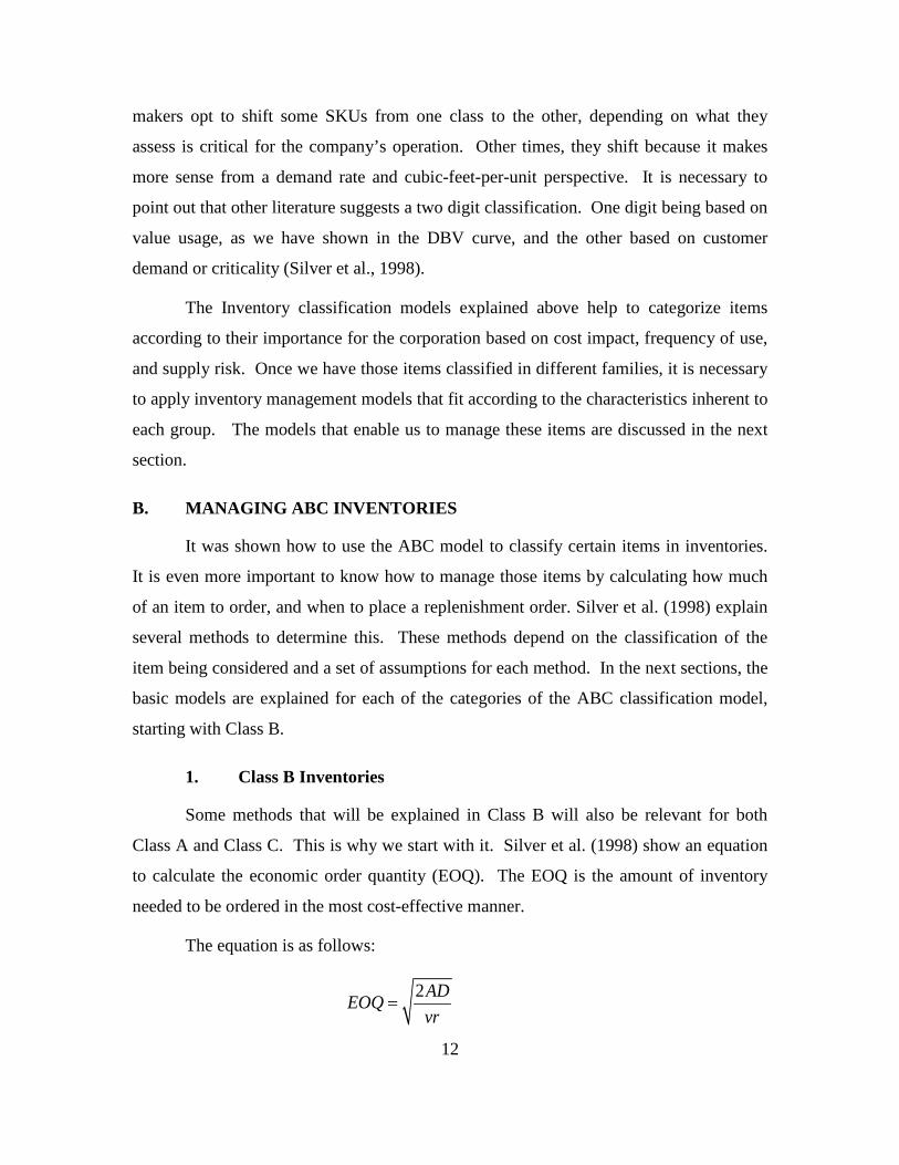
Class A and Class C. This is why we start with it. Silver et al. (1998) show an equation
to calculate the economic order quantity (EOQ). The EOQ is the amount of inventory
needed to be ordered in the most cost-effective manner.
The equation is as follows:
2ADEOQ
vr=

13
where,
A = the fixed cost component in dollars.
D = the demand rate of an item, in units/unit time.
v = the unit variable cost of the item in $/unit.
r = “the carrying charge, the cost of having one dollar of item tied up in
inventory for a unit-time interval (normally one year); that is, the
dimensions are $/$/unit time.” (Silver et al., 1998, p. 152)
Sometimes the number derived from this equation cannot be used. Examples
include if the item ordered has a shelf life, a warranty expires, or if the storage has a
limitation on capacity. Furthermore, the supplier may require a minimum amount of
items to be ordered. The quantity then must be altered depending on these considerations
(Silver et al., 1998).
This EOQ equation assumes that the demand rate is constant. However, if the
demand rate is not constant, then D should be replaced by average demand accumulated
over different periods.
To calculate the reorder point, which is when we should place the order, we use
the following equation:
s = x̄L + kσdLT
where,
x̄L = average forecasted demand during the lead time
kσdLT = Safety stock
and,
k = safety factor (this will be discussed further in the service level section
of the literature review.)

14
σdLT = standard deviation of demand forecasts and lead time, in units.
However, this equation assumes that both demand and lead times are normally
distributed.
2. Class A Inventories
As discussed earlier, Class A inventories are the most important kind of
inventories. There are fewer items in this class than the other classes, but items in Class
A consume most of the dollars and/or demand. Some items are shifted to Class A from
other classes because of other reasons that managers consider critical for the company.
According to Silver et al. (1998), there are guidelines for controlling type A items.
These guidelines are as follows:
1. To use a manual rather than a computer system for records. Manual systems, like Kardex or VISI-Record, are good examples.
2. Frequent inventory reports should be shown to top management for careful inventory revision on a periodic basis.
3. Estimate and influence demand by: a. Providing input by forecasting manually. An example of this is
getting an advance notice of your customer needs. b. Establishing predictability of demand. This can be done using
various methods. For example, when demand is known or scheduled, there is no need to keep a stock of the item needed. On the other hand, when demand is not known, it sometimes makes sense to keep some stock of the items, even if it is expensive. It also makes sense to share some stock with different companies within the same industry on some items of high value and unknown demand.
c. Changing the demand pattern by negotiation with customers, making efficient shipping decisions, and altering price structures, etc.
4. Estimate and influence supply by not only accepting the status quo, but by always negotiating with the supplier to reduce lead time and variability.
5. Be very conservative in stocking this class of items because overstocking can be very expensive.
6. Review order points and quantities frequently because changes might be of costly consequences.
7. Determine order quantities as precisely as possible, due to the importance of Class A items.

15
8. Estimate the cost of shortages in determining levels of safety stock, including the cost of emergency air shipments, of expediting from both in-house and out-of-house sources, and other actions.
Approaches for Class A items that have a high enough average demand in a lead
time (more than 10 units) is discussed in the Class B inventories section because the same
approach can be applied. However, if the average forecast demand in a lead time is
below 10 items, then a discrete distribution, like the Poisson, should be used. This is
because these types of items require a more accurate calculation. The remainder of this
section is concerned with addressing the simultaneous determination of the safety factor
and quantity for the faster movement of Class A items. (Silver et al., 1998).
In the next equations, it is assumed a shortage cost per unit short and a normal
lead time demand. The equations are for an unknown quantity and safety factor. To
calculate the correct quantity to order and safety factor for these types of items, the
following equations should be used (Silver et al., 1998, p. 352):
and
where,
A = fixed cost component incurred with each replenishment
D = annual demand
B2 = fixed cost fraction per unit short
v = unit price
σL = standard deviation of lead time demand
Gu= a function of the unit normal variable
k = safety factor
22 ( )L uAD DB v G kQrv
σ+=
2
( )uQrp kDB
≥ =
16
pu≥ (k) = a function of the unit normal variable (1 – service level)
r = carrying cost
Q = order quantity
To calculate the reorder point(s):
s = x̄L + kσL
This reorder point equation does not differ from the method shown in the Class B
section.
3. Class C Inventories
Silver et al. (1998) note that Class C items represent a large portion of the
inventory, but only consume a low value of the inventory in the company. However, it is
always important to keep in mind that even low value items can have severe shortage
consequences associated with Class C items. One example is that a shortage in Item 1
can cause delay in the usage of Item 2, because it is dependent on Item 1. This may
affect future dealings with this customer. If this customer was important, the effect on
the company could be even bigger. Another example is that even when an item is low in
dollar value, it still may hold a sentimental value for the customer’s president. These
items could then have a high implicit cost associated with a shortage.
It is important to establish principles for Class C items that keep control costs as
low as possible. It is not too much of an investment to try to control Class C items when
their value is very low compared to items in other classes of inventory. This can be
achieved by keeping labor and paperwork to a minimum. Reliance on electronic
equipment for most of the control costs and data capturing is recommended. Records for
Class C items should be kept in the least expensive way; manually or electronically
(Silver et al., 1998). We should note that the classification of an item as Class C should
always be open to revision. This avoids the downgrading of important items to a Class C
status (Silver et al., 1998).

17
To calculate the reorder quantity and reorder point for Class C items, the same
equations shown in the Class B section should be applied.
The factors used in the equations above can be found in the historical data of the
company; however, a service level, which is also included in the equations, must be
either assigned arbitrarily or calculated. In the next section, we show some possible
approaches to calculating it.
C. CUSTOMER SERVICE
There are many definitions of customer service. However, all of them agree when
it comes to the goal of customer service. The goal is the fulfillment of customer needs
using the tools available in the best way. There is a definition for customer service from
the International Customer Service Association. Rinehart, Cooper, and Wagenheim
(1989) define “customer service as those functions within a business that have customer
satisfaction as their responsibility and provide that satisfaction through the fulfillment of
sales order demand and/or information needs” (p. 64).
Customer service levels could be defined as the percentage of orders, which
customers receive on time. This percentage is fundamental for the determination of safety
stock levels. This determination is going to provide satisfaction to the customer and is
considered a success factor.
There are some problems that arise with the definition of service level,
specifically, with the setting of a perfect, feasible, and cost-effective percentage. Another
problem is the identification of the inventory required to obtain the service level we are
seeking.
According to Ettl, Feigin, Lin, and Yao (2000), it is difficult for asset managers to
calculate and decide about the trade-off between the service levels the company wants to
offer its customers, and the investments the company requires on inventory, in order to
attain the service levels expected.
In the next two sections, we explain two existing approaches to the calculation of
service levels we found. One approach focuses on how to assign a service level target,

18
and the other provides a way to determine a cost-effective customer service level. We
analyze these approaches in order to determine which best suits our project.
1. The Service Level Target
There are common mistakes in the process of setting perfect service levels. In
some companies, the service level used to calculate optimal stock levels is given
arbitrarily. Sometimes it is based on past management experience, intuition, or it is based
on agreed goals with customers.
Coleman (2000), in a journal article about how to determine the correct stock
level, provides a four step procedure to determine it. He takes into account relevant
information and some of the most important factors in safety stocks.
In the first step, Coleman (2000) calculates the optimal number of stockouts,
which is given by the holding cost per unit and the shortage cost per unit. However, one
important assumption is that the shortage costs are identified. The equation is as follows:
Optimal Number of Stockouts = Holding Cost per Unit per Year
Shortage Cost per Unit
The second step given by Coleman (2000) is to calculate the number of cycles each year,
which is given by the average annual demand and the order Quantity. The relationship
between these two variables, in addition to the number of orders cycles, indicates the
number of resupply lead times for a year. However, this equation assumes that there is
certain regularity or frequency in the replenishment cycle. The third step is to calculate
the ratio between the equations of step one and two. The equations are as follows:
Number of cycles per year = Average Annual Demand
Order Quantity
Probability of stocking out during each order cycle = Optimal Number of Stockout Occasions Each Year
Number of Exposures to Stockout Each Year
19
Since the third step is the probability of stocking out during each lead time, the service
level, which is the opposite, is calculated as:
Service Level = 1 - Optimal Number of Stockout Occasions Each Year Number of Exposures to Stockout Each Year
The combinations of all these equations yield a single one. This equation contains
the variables not only to calculate it, but, to analyze how the change on any of the factors
would affect the service level. According to Coleman (2000), it is also useful to calculate
the shortage cost for a given arbitrary service level. If the shortage is unknown (which is
an important assumption in Equation 1), managers can use the equation backwards to
determine if the resulting shortage cost is logical.
The final equation, according to Coleman, is as follows:
Service Level = 1 - (Holding Cost per Unit per Year) (Order Quantity) (Shortage Cost per Unit) (Average Annual Demand)
In addition, these variables are to be revised depending on the type of material,
type of business, and the characteristics of the supply chain parties involved. These
characteristics are to be based on the selected classification model.
2. Cost-Effective Customer Service Level
Jeffery, Butler, and Malone (2008), in a research paper about how to determine a
cost-effective customer service level, identify different variables that can be used to
determine equations for customer service levels and the cost associated with achieving it.
In order to determine the customer service level, Jeffery et al. work on two classes
of logistic regression models. These models allow a binary dependent variable that
indicates if an order was late or on time. One class is the planning model that quantifies
the historical relationship between inventory and delivery performance, which is service
level. The other class is the insight models that are developed to analyze the effects of

20
different factors such as lead time, demand variability, and forecast error on the product
group performance. It is necessary to analyze these factors because they have an
important impact on customer service, and the changes they create can be determined. It
is also important because it will enable organizations to analyze the benefits of focusing
efforts on certain improvements.
Because of the relationship between inventory level and the demand forecast,
Jeffery et al. (2008) work with an independent variable called “weeks of inventory.” This
is calculated (along with the three insight models), using the following equations:
Weeks of Inventory (WOI) = Inventory on hand Demand forecast per week
Forecast error = absolute ( Forecast demand – Actual demand ) Actual demand
Order lead time = Requested delivery time – Order placed date
Coefficient of variation of demand = σ of demand for product i μ of demand for product i
Subsequent to the equations above, Jeffery et al. (2008) developed an equation to
calculate the cost of providing a certain service level according to the inventory level
needed for each given one. The cost equation includes holding costs such as
warehousing, obsolescence, scrap, and opportunity costs. It also includes a lost sales cost,
which is obtained using a survey with customers. In this particular case, they indicated a
twenty percent likelihood to move to other suppliers if a product is not delivered on time.
Of course, this percentage of migration to other companies is the result of a
particular case analyzed by Jeffery and the other authors in their research paper.
However, this portion of lost sales must be restated in the analysis of this project. The
reason for this restatement is that there is no option for the customers in the shipyard to

21
migrate (for a single product) to other suppliers, due to the availability of global services.
This situation only happens in a few situations for large equipment or very expensive
items that are only required in very limited quantities.
The equation for the cost of service level, according to Jeffery et al., is given as
follows:
Cost of service level = Inventory units per period*Inventory Holding Cost per unit + expected lost sales units per period * profit margin per unit
Similarly, the holding cost is a function of the Weeks of Inventory, the forecast, and the
different costs incurred with the inventory.
Finally, the optimal cost-effective customer service level is found by plotting the
points of cost and service level for each week of inventory. The optimal service level is
selected according to the lowest cost. As an example, Figure 3 shows a relationship
between inventory, customer service level, and cost for a give product—to which
effective customer is achieved with 3.6 weeks of inventory.
Figure 3. Example of Relationship between Inventory, Cost and Customer Service Level (From Jeffery et al., 2008, p. 230).
22
D. SUMMARY
The overall procedures needed to implement inventory strategies were covered in
this chapter. First, we described the Kraljic and the ABC classification models used to
group the different kind of items in our inventory. The Kraljic model classifies the items
based on cost impact and supply risk. We use Kraljic model to select small sample of
items for detailed study. ABC model classifies the items based on cost impact and usage
frequency. Then, we explained inventory management models and the equations used in
each one. For each class of the ABC model, we assign the adequate equation to be used.
As mentioned above, most of the data needed to apply this model is available—except
the data for service level.
To avoid assigning an arbitrarily service level, we showed two methods to
determine service level. One shows the way to assign a service level and the other shows
how to determine a cost-effective customer service level. These methods give an
accurate service level based on the cost assessment due to stockout risks. The second
approach uses the expected lost sales during the period as a variable to determine the
service level. Because lost sales are not applicable to the inventory we study, we decided
to use the first approach explained in this section.
In the next chapter, we apply the procedures explained in this chapter to the data
collected from COTECMAR to develop the best inventory strategies. For the
classification of the items, the models are applied as explained.

23
II. DATA COLLECTION
This chapter covers the selection of items and their classification. This data is
collected from COTECMAR’s ERP. First, the selection of an adequate sample of items
is covered. This selection is made from an existing classification in the corporation
database on the criticality of the items (Kraljic model) by Diaz and Leaño (2009). Then,
the selected items are organized according to the ABC classification model and listed in a
stock-keeping unit table by descending value. This classification allows us to apply
models to each class in a subsequent section.
A. SELECTION OF THE ITEMS
As a starting point, we take a COTECMAR research report (Diaz & Leaño, 2009)
in which the authors classify goods and services according to the Kraljic model. The
Kraljic model is used primarily to determine purchasing strategies and portfolios.
Although this classification was made in order to classify the vendors and suppliers of the
corporation, it is useful because the items are classified according to some similarities in
their characteristics. As discussed above, these characteristics affect directly or
indirectly the parameters and variables we use for inventory management calculations.
The Goods Supply Matrices (Figures 4 and 5) show the classification of goods by
family2 according to their impact in cost and supply risk. Most of the items are classified
the same way, whether they are used for repair or shipbuilding activities. However, there
are a few differences in the classification of some family items due to their nature of use.
For example, steel is needed in large quantities in shipbuilding for the production of the
complete hull of a given vessel; in contrast, for repair purposes, steel is seldom needed,
and then, only in small quantities. The classifications are shown in Figures 4 and 5.
2 Family here refers to a category of items. For example, the Pipes family includes several different
sizes, lengths, and materials (cooper, steel, plastic) of pipes.

24
Figure 4. Goods Supply Matrix for Repairing and Maintenance (From Diaz & Leaño 2009, pp.42–43, after translation)
Figure 4 shows the item families in each quadrant for repair and maintenance
activities. These activities are offered by the plants for both Navy fleet and civilian
customers. In each family there are a large number of items, and each item has many
different sizes, colors, shapes, weights, references, lengths, measures, and so forth—for
each of the thousands of items used in several kinds of vessels.
The classification used for items related to shipbuilding is similar, with some
differences, as shown in Figure 5.
Strategic Specialized equipment and machinery Engines Ship Engines spares and accessories Paint and coatings Refrigeration systems and supplies Syncrolift and dry dock parts
Leverage Steel sheets Steel profiles Pipes Valves Other piping accessories Welding supplies
Prof
it R
isk
Non-Critical Naval accessories Power and pneumatic tools Fabrics, plastics Welding accessories Seals, rubber, resins, chemicals Bearings, electric and electronic supplies Screws, bolts, nuts Industrial gas
Bottleneck Abrasives Armored glasses Manual tools Sandblasting equipment Clothing, industrial safety equipment Cables Cooper slag Furniture for ships
Supply Impact

25
Figure 5. Goods Supply Matrix for Shipbuilding (From Diaz & Leaño 2009, pp.43–44, after translation)
From these groups of families, it is necessary to take a sample to run the models.
As mentioned above, COTECMAR has three basic business lines or divisions:
Bocagrande repair plant (Bocagrande), Mamonal repair plant (Mamonal), and
Shipbuilding. Therefore, we take three items from each quadrant per business line, for a
total of twelve items per business line, and a sum total of thirty-six items.
However, we cannot randomly choose these items because we may choose a very
sporadic item. A sporadic item is not going to provide enough data to accurately analyze,
and would therefore be completely useless. Consequently, it is necessary to select the
items with regard to their usage. The items with a high usage volume are identified for
each quadrant, and described accordingly in Table 3.
Strategic Specialized equipment and machinery Steel sheets Steel profiles Refrigeration systems and supplies Engines Ship Engines spares and accessories Syncrolift and dry dock parts
Leverage Pipes Valves Other piping accessories Paints and coatings Welding supplies
Prof
it R
isk
Bottleneck Armored glasses Filters Sandblasting equipment Clothing, industrial safety equipment Electric and electronic supplies Cables Furniture for ships Manual tools
Non-Critical Power and pneumatic tools Naval accessories Cooper slag Welding accessories Abrasives Seals, rubber, resins, chemicals Screws, bolts, nuts Industrial gas
Supply Impact

26
Bottleneck Items Line Item Family Code Item
Mamonal Clothing and Industrial Safety Eq. 20324674 DIELECTRIC SAFETY BOOTS - SIZE 41
Cables 20006167 RUBBER WRAPPED CABLE 3 X 12 110V
Cooper slag 20473778 MINERAL COOPER SLAG GRANULOMETRY GR-3
Bocagrande Clothing and Industrial Safety Eq. 20324674 DIELECTRIC SAFETY BOOTS - SIZE 41
Cables 20006167 RUBBER WRAPPED CABLE 3 X 12 110V
Cooper slag 20473778 MINERAL COOPER SLAG GRANULOMETRY GR-3
Shipbuilding Armored glasses 20259556 POLYCARBONATE ARMORED GLASS LEVEL 3 LEFT 46X69X 700mm
Clothing and Industrial Safety Eq. 20324667 DIELECTRIC SAFETY BOOTS - SIZE 40
Electric-electronic Supplies 20008420 NON-CONDUCTING TAPE SUPER 33+ 19MM X 20MTS
Non-Critical Items Line Item Family Code Item
Mamonal Naval accessories 20145873 SUPERBRAIDED NYLON ROPE 1.1/2"
Welding accessories 20019969 STONE FOR FRICTION LIGHTER Industrial gas 20041076 AGA SOL
Bocagrande Naval accessories 20401665 FLUORESCENT LAMP IP67 2X18W 120VAC 60HZ REF. 1044216205
Bearings 20023188 BEARING REF. 6205 ZZ C3
Screws 20028060 SCREW HEX GALVANIZED UNC 5/8" X 2.1/2"
Shipbuilding Naval accessories 20050498 NYLON ROPE 3/4" Screws 20055165 SCREW HEX STAINLESS AISI 304
UNC 3/8" X 1" Resins 20110017 WHITE GELCOAT 888
Table 3. Items Sample Selected per Quadrant per Business Line

27
Strategic Items Line Item Family Code Item
Mamonal Paints 20085926 ADJUSTER FOR EPOXY PAINT REF. 121135
Paints 20036409 CATALYST FOR POLY EPOX REF. 9800 (13227)
Pains 20021320 ANTICORROSIVE POLY EPOX RED REF. 9101 (210050)
Bocagrande Paints 20007560 CATALYST FOR POLY EPOX REF. 9800 (13227)
Paints 20020118 POLI EPOX GREY REF. 9600 (213222)
Refrigeration systems and supplies 20038557 FREON 22
Shipbuilding Steel (sheets and profiles) 20001513 ANGLE C/S 1/4" X 2" Steel (sheets and profiles) 20020545 PLATE C/S ASTM A-36 1/4" X 2"
Steel (sheets and profiles) 20057909 GALVANIZED SHEET ASTM A-366 GAUGE 20 X 4' X 8' (1.22MTx2.44MT)
Leverage Items Line Item Family Code Item
Mamonal Steel (sheets and profiles) 20269746 NAVAL STEEL SHEET ASTM A-131 3/8" X 8' X 20' (WEIGHT: 1113.0KG)
Pipes 20068257 FLANGE SLIP ON 6" 150 LB C/S ASTM A105 RF
Welding accessories 20183202 WELDING AWS E7018 1/8"
Bocagrande Steel (sheets and profiles) 20001513 ANGLE C/S 1/4" X 2"
Pipes 20029098 PIPE C/S 1" SCH 40 SEAMLESS
Welding accessories 20183271 WELDING AWS E7018 3/32"
Shipbuilding Pipes 20029098 PIPE C/S 1" SCH 40 SEAMLESS Paints 20085926 ADJUSTER FOR EPOXY PAINT REF.
121135 Welding accessories 20183295 WELDING AWS E7018 5/32"
Table 3 (continued). Items Sample Selected per Quadrant per Business Line
In order to get the data we need for calculation purposes, we downloaded several
files from the ERP software. Infor XA is the maker of the ERP system used by
COTECMAR. In this software, COTECMAR employees enter the data in order to make
transactions according to each division or department. For instance, the Human
28
Resources Department enters data related to wages, primes, labor, etc. The Production
Department enters data such as working hours, and they also do their material
requisitions through the system. The Purchasing division does Purchase orders in the
system. The Warehouse Division performs all material movements and transactions in the
system. Accounting does the billing, cost, and all of the accounting transactions in the
system. Thus, we can rely on this software to download the data we need, according to
the information we want. The source of the specific data used is detailed for each
equation or analysis performed.
In the previous section, the items have been selected from the Kraljic model in
use at COTECMAR, taking into account items with substantial information that will
allow us to perform a good analysis. In the next section, these selected items are
classified according to the ABC model and listed in a stock-keeping unit table in
descending value.
B. DATA GATHERING
In order to analyze our sample we need to gather various data. The total number
of items for data gathering and analysis is 35. The sample was 36 items, but the item
ADJUSTER FOR EPOXY PAINT REF. 121135 for Mamonal and Shipbuilding has the
same warehouse location so they are treated as a single item instead of two items. Some
of the other items are also the same in Mamonal and in Bocagrande, but they have
different inventory locations, and this characteristic makes them different SKUs. For
simplicity, and because Mamonal and Shipbuilding are co-located, demand for Mamonal
and shipbuilding will be treated the same.
In the SKU table, the cumulative percentage is calculated by adding the
percentage of each SKU. The percentage for each SKU is calculated by dividing 100%
by the total of SKUs, which is a total of about 2.86% per SKU.
For the calculation of the Annual Usage we need two values: the Annual Demand
and the Unit Price. For the Annual Demand, we compare the information in three files
downloaded from the ERP System. We have information from January 2006 to January
2012, although some files only contain information from January 2008 to January 2012.

29
The first file is the Requisition record, where we have the following information
for each transaction: requisition number, class or family of material, code of the item,
name of the item, quantity, unit of measurement (i.e., units, pounds, gallons), name of the
project, cost center, requisition date, and date required. Extra information from the
system, due to the correlation with the transactions from other divisions and departments,
is unnecessary.
The second file is the Purchase Orders (PO) record. Here, we have PO number,
item codes, item name, warehouse the item goes, unit of measurement, quantity, unit
price, total price, PO date, delivery date, and supplier name. As before, the extra,
unnecessary information is ignored.
Finally, the third file is the Warehouse (WH) Transactions records. In this file, we
have the quantity, the transaction (entrance, delivery, return, entrance from consignment,
transfer), item code, warehouse (Bocagrande, Mamonal), item name, unit cost, date, and
balance quantity. Extra unnecessary information is also ignored here.
For the analysis, we leverage the data collected from the first file—the
Requisition Record—and we get the average demand quantity per year from 2008 to
20113. We do the same with the PO record from 2006 to 2011, and the same with the
WH transactions record from 2008 to 2011, and we come with an average with high
variation. The reason for this high variation might be the variation in the type of projects
and the different technologies used in the steel works.
For the price calculation, we take two averages: the average price from the PO
Records file over the years and the average from the WH transactions file. We obtain a
similar price number with small variation between one file and the other.
The remaining information in the table is the cumulative usage and the cumulative
percentage of the total usage, which is simple to calculate once we complete the annual
usage column and we order the items in descending value.
3 In all cases 2012 data is ignored in order to compare complete annual data.
30
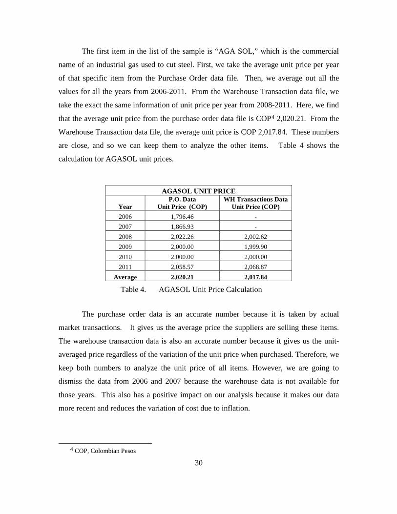
The first item in the list of the sample is “AGA SOL,” which is the commercial
name of an industrial gas used to cut steel. First, we take the average unit price per year
of that specific item from the Purchase Order data file. Then, we average out all the
values for all the years from 2006-2011. From the Warehouse Transaction data file, we
take the exact the same information of unit price per year from 2008-2011. Here, we find
that the average unit price from the purchase order data file is COP4 2,020.21. From the
Warehouse Transaction data file, the average unit price is COP 2,017.84. These numbers
are close, and so we can keep them to analyze the other items. Table 4 shows the
calculation for AGASOL unit prices.
AGASOL UNIT PRICE
Year P.O. Data
Unit Price (COP) WH Transactions Data
Unit Price (COP) 2006 1,796.46 - 2007 1,866.93 - 2008 2,022.26 2,002.62 2009 2,000.00 1,999.90 2010 2,000.00 2,000.00 2011 2,058.57 2,068.87
Average 2,020.21 2,017.84
Table 4. AGASOL Unit Price Calculation
The purchase order data is an accurate number because it is taken by actual
market transactions. It gives us the average price the suppliers are selling these items.
The warehouse transaction data is also an accurate number because it gives us the unit-
averaged price regardless of the variation of the unit price when purchased. Therefore, we
keep both numbers to analyze the unit price of all items. However, we are going to
dismiss the data from 2006 and 2007 because the warehouse data is not available for
those years. This also has a positive impact on our analysis because it makes our data
more recent and reduces the variation of cost due to inflation.
4 COP, Colombian Pesos

31
The second step is to calculate the demand. For this, we take the Requisition data
file and add all of the quantities for each year. Then, we average out the totals of each
year. We follow the same process with the purchase order data file. Finally, we do the
same with the Warehouse Transaction data file.
In the Warehouse data file, there are multiple kinds of transactions, as follows:
RW - Entrance from Transfer IW - Exit from Transfer IU - Exit to Project IS - Exit for OH or Investment RC - Entrance from Consignment RS - Return from Project VR - Return for PO RP - Entrance from PO
For the purpose of collecting demand data, we only use IU and IS transactions. From this
quantity, we subtract the quantity of RS transactions. The ERP has 44 virtual
warehouses. Some of them are created for specific projects and other are created for
suppliers consignments. Thus, we need to select an adequate set of virtual warehouses
that belong to one of the two sets of physical warehouses located at either Mamonal or
Bocagrande (Table 6 shows all warehouses). After selecting this data, we add all the
quantities for each year. Then we average out the totals of each year, just as we did with
the Requisition and Purchase Order files. One example of this calculation is shown in
Table 5.
AGASOL DEMAND (MAMONAL)
Year Requisition Data Demand
P.O. Data Demand
WH Trans. Deliveries
Returns to WH
Final WH Trans. Data Demand
2006 80,169.00 2007 26,196.00 2008 33,678.70 9,396.00 28,139.50 151.50 27,988.00 2009 99,856.26 44,938.50 39,580.00 1,324.50 38,255.50 2010 117,350.30 64,627.00 31,244.00 809.50 30,434.50 2011 100,654.20 69,605.00 29,091.00 1,341.50 27,749.50 Total 87,884.87 49,155.25 31,106.88
Table 5. AGASOL Demand Calculation in Kilograms

32
As shown in Table 5, average demand per year is very different amongst the date
files. The requisition demand is high because it contains requisitions made from the
warehouse division to the purchase division, as well as requisitions made from the
production department to the warehouse division. Another reason might be that the
production department inflates their actual needs in order to make sure that plenty of raw
materials are available for their use. The purchase order demand is high because it
contains all items purchased for use and for stock. Consequently, the demand from the
Warehouse Transaction data files is more accurate because it gives the actual quantities
delivered to production. Therefore, for all the remaining items, we are only going to use
the Warehouse Transaction data files.
Warehouse Description Physical Location ACT Fixed Assets Warehouse (PPE) Mamonal FCU Virtual Warehouse Frigates (Custody) Bocagrande FRG Virtual Warehouse Frigates Bocagrande MBY Manta Bay Project (Mamonal Km9) Mamonal MLG Virtual Warehouse Malaga Bocagrande OPV Virtual Warehouse OPV Mamonal PAF Light Patrol Project Mamonal PTC Shipbuilding Warehouse (Mamonal Km9)* Mamonal PTM Warehouse Mamonal Plant* Mamonal PV2 Warehouse OPV 2* Mamonal P01 Production* Mamonal S01 Services Mamonal* Mamonal S02 Services Bocagrande* Bocagrande S03 Services Shipbuilding* Mamonal S04 Services Holding* Mamonal
1 Mamonal Mamonal 2 Bocagrande Bocagrande 3 Armored Project Bogota Mamonal 4 Distribuidora Ancla** Mamonal 5 Distribuidora Ancla Bocagrande** Bocagrande 6 Empaquetaduras Y Empaques Bocagrande** Bocagrande 7 Disprotec – Bocagrande** Bocagrande 8 Disprotec- Mamonal** Mamonal 9 Central De Soldaduras Mamonal** Mamonal
10 Central De Soldaduras Bocagrande** Bocagrande 11 Propulsora Mamonal** Mamonal 12 Agafano Bocagrande** Bocagrande 13 Propulsora Bocagrande** Bocagrande 14 Soldarco** Mamonal 15 Tatis Y Cia** Mamonal 16 Pintuco S. A.** Mamonal 17 Pintuco Bocagrande** Bocagrande 19 Central De Soldaduras Mamonal** Mamonal 22 Agafano Mamonal** Mamonal 23 Cryogas** Mamonal

33
24 S. P. Y S. Mamonal** Mamonal 26 Tuvacol S. A.** Mamonal 27 Central De Mangueras** Mamonal 28 Sinco Ltda Mamonal** Mamonal 29 Sinco Ltda Bocagrande** Bocagrande 30 Central De Soldaduras Bocagrande** Bocagrande 32 Empaquetaduras Y Empaques** Mamonal 33 S. P. Y S. Bocagrande** Bocagrande 36 Tuvacol Bocagrande** Bocagrande
*Created on January 1st 2012 **Created with Suppliers Names due to Consignment Inventory (Vendor-Managed Inventory)
Table 6. COTECMAR Warehouses
C. ITEM CLASIFICATION
With the demand and value information, we are ready to calculate the annual
usage from the demand and purchase cost, and then classify the SKUs according to the
ABC model. This information is presented in Table 7 and organized in descending value.
Then, cumulative usage and the cumulative percentage of the total usage are also shown.
No. SKU NAME Cum.
Percent SKU
Annual Usage (Dv)
(COP)
Cumulative Usage (COP)
Cumulative Percentage of
total usage
Item Class
1 NAVAL STEEL SHEET 3% 496,116,781 496,116,781 31% A 2 FLUORESCENT LAMP 6% 156,299,811 652,416,591 41% A 3 WELDING 1/8" 9% 123,649,347 776,065,939 49% A 4 ANTICORROSIVE EPOX 11% 108,374,385 884,440,324 56% A 5 MINERAL COPPER SLAG 14% 91,134,607 975,574,931 61% B 6 ADJUSTER FOR EPOXY 17% 81,797,032 1,057,371,963 66% B 7 MINERAL COPPER SLAG 20% 72,559,112 1,129,931,075 71% B 8 CATALYST FOR EPOX 23% 72,078,714 1,202,009,789 76% B 9 WELDING 5/32" 26% 70,282,098 1,272,291,886 80% B 10 AGA SOL 29% 62,805,626 1,335,097,513 84% B 11 CATALYST FOR EPOX 31% 50,937,762 1,386,035,274 87% B 12 POLY EPOX GREY 34% 31,399,074 1,417,434,348 89% B 13 SAFETY BOOTS SIZE 40 37% 19,573,832 1,437,008,180 90% B 14 ANGLE C/S 1/4" X 2" 40% 18,103,281 1,455,111,462 91% B 15 WHITE GELCOAT 43% 15,552,737 1,470,664,199 92% B 16 SAFETY BOOTS SIZE 41 46% 15,145,864 1,485,810,063 93% B 17 ANGLE C/S 1/4" X 2" 49% 14,811,776 1,500,621,839 94% B 18 FLANGE SLIP ON 6" 51% 11,320,631 1,511,942,470 95% B 19 SUPER NYLON ROPE 54% 9,525,719 1,521,468,189 96% B 20 GALVANIZED STEEL SHEET 57% 9,367,134 1,530,835,323 96% B 21 WELDING 3/32" 60% 8,679,333 1,539,514,656 97% B 22 SAFETY BOOTS SIZE 41 63% 7,457,074 1,546,971,730 97% C 23 NON-CONDUCTING TAPE 66% 6,545,589 1,553,517,319 98% C

34
24 FREON 22 69% 6,296,730 1,559,814,049 98% C 25 PLATE C/S 1/4" X 2" 71% 5,627,581 1,565,441,630 98% C 26 PIPE C/S 1" SEAMLESS 74% 5,487,622 1,570,929,253 99% C 27 SCREW HEX GALVANIZED 77% 5,162,920 1,576,092,172 99% C 28 CABLE 80% 5,145,051 1,581,237,223 99% C 29 PIPE C/S 1" SEAMLESS 83% 4,792,233 1,586,029,456 100% C 30 ARMORED GLASS 86% 1,724,951 1,587,754,407 100% C 31 CABLE 89% 1,661,624 1,589,416,031 100% C 32 SCREW HEX STAINLESS 91% 739,490 1,590,155,521 100% C 33 NYLON ROPE 3/4" 94% 425,544 1,590,581,065 100% C 34 STONE FOR FRICTION 97% 334,938 1,590,916,003 100% C 35 BEARING 100% 306,642 1,591,222,645 100% C
Table 7. Listing of Sample SKUs by Descending COP Usage
Figure 6 shows the distribution of SKUs by value. This figure is based on the
values from Table 7. We can see from this figure—and the table—that the figure follows
the regular distribution for industrial goods, of which about 26% of the SKU account for
about 80% of the total annual COP usage. Thus, not all of the inventory should be
controlled to the same extent. This is why we use the ABC classification model, as
suggested by Silver et al. (1998).
Figure 6. Distribution of SKUs by value
0%
20%
40%
60%
80%
100%
0% 20% 40% 60% 80% 100%
Perc
enta
ge o
f Tot
al A
nnua
l CO
P U
sage
Percentage of Total of SKU

35
With Table 7, we can classify inventories based on importance. The most
important inventories (rated A) are located in positions 1 to 4, because they represent
about 11% of the total SKU and account for about 56% of the total annual COP value.
The second most important items (in relation to Class A items) are Class B items, which
are located in positions 5 to 21. These B items represent about 49% of the total SKU and
account for 41% COP usage, which is most of the remaining annual COP usage. Finally,
the least important are Class C items, because they represent a very small part of the total
COP investment. The Class C items are located in positions 22 to 35. These items
represent about 40% of the total SKU and account for only 3% of the total COP usage.
In the previous sections, we have selected the items based on the Kraljic model
from existing research made in COTECMAR. The items are selected by taking into
account those that have enough good information to apply the models, and thus make
valid inferences about the whole category of items. Furthermore, the selected items have
been classified according to the ABC classification model, and are listed in a SKU table
in descending value. From this table, we take the items A, B, and C, according to the
percentage of dollar usage and the cumulative percentage of SKUs.
In the next chapter, we discuss inventory strategy models for each class of items,
and determine the variables needed for each equation. For the inventory management
models, assumptions and rules are addressed. For the service level calculation, the
correct service level is determined in order to maintain a level that satisfies customer
needs based on stockout costs.

36
THIS PAGE INTENTIONALLY LEFT BLANK

37
IV. INVENTORY ANALYSIS
This chapter covers the determination of the variables that will be needed for
inventory management calculations. Moreover, this chapter includes discussion of
different inventory models, along with the assumptions related to each one and the
selection of the appropriate model. Furthermore, this chapter goes over the application of
the data in all of the equations. Finally, at the end of this chapter, all of the findings are
listed. In the following chapter, working from these calculations and findings, we present
conclusions and recommendations.
A. DEMAND RELATED ANALYSIS
In this section, we determine the variables to be used in the equations and explain
how each one is calculated using the existing data.
1. Demand
In this section, we explain the big picture and demand patterns—the behavior of
the demand—in COTECMAR. We also determine what kind of data or information
related to the demand is useful for the purpose of our research scope. COTECMAR’s
projects—shipbuilding, overhauling, and repairing—have an important impact upon the
behavior of the demand. With these kinds of projects, the demand for items is at times
sporadic and at other times regular. These characteristics belong to both dependent
demand items and independent demand items. Therefore, we first define dependent
demand items and the process to manage them. Then, we turn to our research focus to
the definition of independent demand items and the process to manage them. Finally, we
explain the calculation of demand for items that have independent demand, in order to
use it in the equations for this project.
According to the big picture of the calculated demand in the “Organization of the
Items” section for the SKU table, we find that some of the items have abnormal
variation—different from regular variability, seasonality, or normal patterns. Some items
38
have annual demands that are fairly constant. Other items have very high variability.
Items with high variability either show no particular pattern, or have a pattern that
increases over time.
We attribute abnormal variation to specific projects that have a dependent demand
and go over a predetermined span of time. For example, when COTECMAR receives an
order to build a new ship, the demand for steel sharply increases in the first phase of the
shipbuilding process. This is because the complete hull is built in the first phase. When
the hull is completed, the demand for steel returns to its normal position. However, the
demand for pipes, in the second phase, sharply increases during the outfitting process.
Again, the demand for pipes goes back to its normal position after this phase is
completed, and so on for all of the items that are going to be used for that specific
shipbuilding project. For this kind of item, different approaches from the regular EOQ
and ROP models are applied. According to Silver et al. (1998), materials requirement
planning (MRP) is an approach to manage this kind of demand. The MRP approach is
explained in the dependent demand items section below.
Based on the characteristics of the demand we observe in the data, we consider it
necessary to determine whether the demand belongs to dependent demand items or to
independent demand items. The literature review does not cover this classification
method, but it is necessary to determine this because, depending on this classification,
either the inventory models or the MRP approach is more appropriate. In order to
understand the concepts of dependent and independent demand items, we explain them as
follows.
a. Dependent Demand Items
According to Baily (1987), dependent demand items are items that depend
on demand for the product scheduled to be produced. Baily (1987) adds that different
methods, such as demand forecasting using moving averages and exponential smoothing,
are not appropriate and lead to either shortages or excessive stocks. The calculation of
order quantities, in the way it was applied to other types of items, is also not appropriate
for these items.
39
Silver et al. (1998) talk about this in the explanation of multi-echelon
situations, in which “any specific piece of equipment requires a particular set of
components” (p. 511). In COTECMAR, specific projects—such as shipbuilding,
overhauling, transformation, or dismantling—require specific items unique for those
projects, or a certain quantity of regular items that go beyond the regular quantity
demanded. Although these specific projects are part of the ordinary business, they are
known in advance and make it possible to conduct a replenishment plan. This is not the
case for the repair process, in which the items or materials that are needed are determined
once the technicians are already working on the system.
For dependent items, “requirements for parts and materials for the
manufacture of a product to meet production schedules should be planned together as a
single group, not as a lot of independent individual items. This is called Materials
Requirement Planning (MRP).” (Baily, 1987, p.120)
MRP can involve thousands of items that have complications, such as
varying lead times and demand. The first step of the MRP process is to establish a master
production schedule, which is a planned out schedule showing what products, and what
quantities of them, are needed to be completed by what dates. This schedule is usually
listed on a weekly basis for three months, and then on a monthly basis for the next nine
months. (Baily, 1987)
Then, the master production schedule should be expanded and include a
detailed requirement of all the items needed to create each product. This is done by
establishing the Bill of Materials (BOM). The Bill of Materials for a particular product
lists all of the items needed, along with their quantities, to produce this specific product.
It is sometimes referred to as the parts list. The Bill of Materials should be done on each
product listed in the master production schedule. The planning of item ordering for the
net requirements of each product should take into account the lead time needed, so that
the items ordered arrive on time for production to meet the required date to finish the
product (Baily, 1987). This is the way that MRP deals with dependent demand items.
40
b. Independent Demand Items
This project focuses on independent demand items data for the application
of the models. According to Zipkin (2000), independent demand items are those for
which there is no supply-demand link between them, and their processes are different.
These items satisfy the assumptions of the EOQ model (or, if some of the assumptions
are violated, these violations may be relaxed in some way). Items with this attribute are
required on a regular basis for some production processes, mostly for repairs. Therefore,
the demand does not depend on a special or temporary situation. Concurring with Zipkin
(2000), we can control each of these kinds of items, separately from the others, and apply
the EOQ and ROP models and control the inventory with the obtained results.
In order to refine the demand data, it is necessary to remove the items that
belong to specific projects, such as shipbuilding or overhauling, since this constitutes
dependent demand. For this purpose, we analyze each of the items in the Warehouse
Transactions data file. There are columns in this file that provide information for the
project code, project name, transaction reference, and work order. However, there is a
lack of information in some of the important columns, such as project name, due to the
incomplete fields that warehouse employees sometimes leave when they are registering
the transactions.
We use tools such as Excel pivot tables to determine what projects are a
part of larger projects that represent dependent demand. The pivot tables give us the
percentage of consumption of each project out of the total demand. High percentages of
consumption are looked into more carefully, because they may belong to large projects.
With this information, we review the data to find the name or type of project. Some
projects have a single project code. Other projects have multiple project codes for several
reasons: because they are related to two or more vessels, because they are done in
multiple stages, or because they have different work areas on the same project (i.e., fresh
water system and propulsion system). Another characteristic of these kinds of projects is
that they span a long period; most of the time they last more than six months. Based on
our examination of the data, we found the following projects, with their codes, that have
been completed during the period that our data covers. These projects are determined to

41
have dependent demand; therefore, they drive the demand according to their own Bill of
Material, so inventory to meet this demand can be ordered in advance, according to the
MRP approach. Thus, in order to focus on our research project scope—independent
demand items, the following projects are removed from our demand data:
• Submarines-overhauling: 855, 796.
• Support River Patrol (PAF)-shipbuilding: 296, 297, 845, 846, 903, 920.
• “Vicky B” - double hull: 539.
• Frigates-overhauling: 102, 113, 123, 125, 128.
• Offshore Patrol Vessel-shipbuilding: 840, 1002, 1082.
• “Manta Bay” Tanker Vessel-Overhauling: 1064.
• River Patrol Boat-shipbuilding: 828, 835, 836, 837.
Furthermore, all investment projects (such as road pavement or facility
construction) are also excluded for the same reason as the projects above: these
investments are planned in advance, so it is possible to conduct replenishment planning.
We do not find projects of this kind by analyzing information about consumption. These
projects do not have work orders like repair or shipbuilding projects. However, they have
an administrative cost center that is characterized with a letter “P,” and a four-digit
number that always begins with “6” (i.e., P6497).
The remaining data relates to repair processes. These projects are short in
execution and occur fairly regularly over time, without enough advanced notice for
planning. There are two different kinds of situations with repair projects. One is that
demand for repairs is not known in advance. The other situation is that the parts required
for each repair are not known until the process starts or is underway. These repairs are the
source of the independent demand items. We treat them as independent because they do
not have the predictability and advanced notice of demand like the shipbuilding projects.
After filtering the data, we see all the data for each item via their
transaction records. We group all the transaction records by month to determine monthly
demand and monthly standard deviations for all of the items. With these groupings, we
have demand with a time measure, and we can scale it to any time unit of measurement

42
we could need for our calculations (i.e., daily, weekly, or annual demand). Table 8
shows the average monthly demand, standard deviation, and the coefficient of variation
for each of the items. Note that, once the dependent demand quantities were removed, no
independent demand for Mineral Copper Slag remained at Mamonal (Item 5). For this
reason, this item is removed from the items that are going to be analyzed using EOQ
model in the next section.
ITEM NAME WAREHOUSE AVERAGE STDEV CV 1 NAVAL STEEL SHEET Mamonal 10,317.53 12,793.66 1.24 2 FLUORESCENT LAMP Bocagrande 0.57 2.30 4.03 3 WELDING 1/8" Mamonal 1,241.61 836.04 0.67 4 ANTICORROSIVE EPOX Mamonal 85.29 69.65 0.82 5 MINERAL COPPER SLAG Mamonal 0 0 0 6 ADJUSTER FOR EPOXY Mamonal 23.82 11.64 0.49 7 MINERAL COPPER SLAG Bocagrande 13,207.75 13,631.47 1.03 8 CATALYST FOR EPOX Mamonal 113.41 86.87 0.77 9 WELDING 5/32" Mamonal 807.49 636.57 0.79
10 AGA SOL Mamonal 1,547.76 1,001.81 0.65 11 CATALYST FOR EPOX Bocagrande 55.81 43.10 0.77 12 POLY EPOX GREY Bocagrande 7.02 22.71 3.23 13 SAFETY BOOTS SIZE 40 Mamonal 13.84 13.03 0.94 14 ANGLE C/S 1/4" X 2" Mamonal 5.04 11.73 2.33 15 WHITE GELCOAT Mamonal 20.45 26.25 1.28 16 SAFETY BOOTS SIZE 41 Mamonal 11.73 12.06 1.03 17 ANGLE C/S 1/4" X 2" Bocagrande 4.67 7.14 1.53 18 FLANGE SLIP ON 6" Mamonal 6.51 16.77 2.58 19 SUPER NYLON ROPE Mamonal 21.33 41.07 1.93 20 GALVANIZED STEEL SHEET Mamonal 1.57 5.70 3.63 21 WELDING 3/32" Bocagrande 21.41 26.40 1.23 22 SAFETY BOOTS SIZE 41 Bocagrande 7.37 6.26 0.85 23 NON-CONDUCTING TAPE Mamonal 16.94 17.59 1.04 24 FREON 22 Bocagrande 39.80 46.87 1.18 25 PLATE C/S 1/4" X 2" Mamonal 43.88 94.85 2.16 26 PIPE C/S 1" SEAMLESS Bocagrande 11.16 27.34 2.45 27 SCREW HEX GALVANIZED Bocagrande 7.59 33.73 4.44 28 CABLE Mamonal 19.39 79.59 4.11 29 PIPE C/S 1" SEAMLESS Mamonal 9.95 18.13 1.82 30 ARMORED GLASS Mamonal 0.02 0.14 7.00 31 CABLE Bocagrande 11.94 26.77 2.24 32 SCREW HEX STAINLESS Mamonal 3.27 10.85 3.32 33 NYLON ROPE 3/4" Mamonal 1.10 5.43 4.93 34 STONE FOR FRICTION Mamonal 15.80 15.84 1.00 35 BEARING Bocagrande 1.12 1.63 1.45
Table 8. Average and Standard Deviation of Demand

43
We observe a high variation of demand based on the ratio σL/xL̄ suggested
by Silver et al. (1998). This ratio, shown in the CV column of Table 8, is used in order to
consider using a different approach rather than an approximation for normal distributions.
According to them, if the ratio is greater than 0.5, we should consider using a different
distribution of demand, such as the Gamma. In our analysis, all items—with the
exception of the “Adjuster”—have a ratio greater than 0.5. Most values were significantly
higher than 0.5.
In order to know the distribution, and to test if the normal distribution fits
our demand data, we make some tests using the goodness-of-fit test of the “crystal ball”
risk-analysis software application. This allows us to know the kind of distribution that
best fits the set of observations in our demand data for each item. Furthermore, it shows
us how much (and to what side) the data is skewed.
After drawing all the distribution for all of the items, we find that they
have different kinds of distributions, such as lognormal, weibull, beta, maximum
extreme, and logistic. None of the items have normal distribution. Figures 7 and 8 show
examples of the distribution of two items.
Figure 7. Beta Distribution Goodness-of-Fit test for “Angle” Item Demand

44
Figure 8. Weibull Distribution Goodness-of-Fit test for “Agasol” Item Demand
2. Lead Time
In order to calculate the order lead times, we use the Purchase Order data file. We
filter all purchase orders made for an item, and find the lead time by subtracting the
purchase order creation date from the supplier delivery dates. Lead times from suppliers
have a regular time frame; however, there is some variation (due to unique cases) that
makes it necessary to refine the data.
3. Refining the Data
While going through the immense amount of data we have, we encounter
numbers that are very far from the norm, or outliers. This is especially evident in the data
concerning demand and lead times. This creates a bit of a problem for COTECMAR’s
management, because it distorts the real picture and the outlying numbers affect our
averages greatly. We recognize that some of these outlier numbers are due to typos and
others might be due to extraordinary circumstances. Therefore, we want a way to keep
these numbers out of our calculations, in order to make our averages more realistic.
Instead of removing the numbers in an arbitrary way, we want to follow an
acknowledged procedure to know exactly which numbers we should consider as outliers.

45
According to Keller (2009), there is a way to recognize which numbers are to be
considered outliers within a certain data set. The procedure described can be achieved by
following these steps:
1. Calculate the first (lower) and third (upper) quartiles of a data set.
2. Calculate the inter-quartile range by subtracting the lower quartile from
the upper quartile.
3. Multiply 1.5 by the inter-quartile range.
4. Add the product of step 3 to the upper quartile. This gives you the upper
limit of the numbers you should consider in your data set. Any number
above this should be considered as outlier; hence, it can be discounted.
5. Subtract the product of step 3 from the lower quartile. This gives you the
lower limit of the numbers you should consider in your data set. Any
number below this should be considered as an outlier; hence, it can be
discounted.
For instance, the lead times data set for the item “Copper Slag” are {56, 5, 1, 1,
13, 13, 47, 20, 65, 15, 17, and 97}. The steps to determine the outlying numbers in this
data set are explained in the following process:
1 Upper quartile 53.75 2 Lower quartile 7 3 (upper quartile) - (lower quartile) 46.75 4 [(upper quartile) - (lower quartile)]*1.5 70.125 5 Upper quartile + Product of step 4 123.88 6 Lower quartile - Product of step 4 -63.13
The previous calculation shows that any numbers that are above 123.88 and
below -63.13 can be considered outliers. We can see that we do not have any outlying
numbers in this data set; thus, no numbers should be discounted. We use this method for
all of the data sets that we think are greatly affected by outlier numbers.

46
Table 9 shows the calculated lead times for each item after outliers have been
removed.
No. Name Average Lead Time
Std. Dev. Lead Time
1 NAVAL STEEL SHEET 6.51 6.19 2 FLUORESCENT LAMP 46.20 34.25 3 WELDING 1/8" 3.03 2.82 4 ANTICORROSIVE EPOX 6.11 3.54 5 MINERAL COPPER SLAG 29.17 30.23 6 ADJUSTER FOR EPOXY 5.60 3.17 7 MINERAL COPPER SLAG 29.17 30.23 8 CATALYST FOR EPOX 6.31 3.58 9 WELDING 5/32" 2.76 2.78
10 AGA SOL 3.36 2.94 11 CATALYST FOR EPOX 6.31 3.58 12 POLY EPOX GREY 7.33 4.24 13 SAFETY BOOTS SIZE 40 22.18 19.97 14 ANGLE C/S 1/4" X 2" 3.86 2.94 15 WHITE GELCOAT 7.37 4.65 16 SAFETY BOOTS SIZE 41 22.56 19.58 17 ANGLE C/S 1/4" X 2" 3.86 2.94 18 FLANGE SLIP ON 6" 3.50 2.79 19 SUPER NYLON ROPE 8.18 7.56 20 GALVANIZED STEEL SHEET 6.34 5.34 21 WELDING 3/32" 2.40 1.43 22 SAFETY BOOTS SIZE 41 22.56 19.58 23 NON-CONDUCTING TAPE 5.09 3.80 24 FREON 22 4.25 4.00 25 PLATE C/S 1/4" X 2" 3.47 2.75 26 PIPE C/S 1" SEAMLESS 4.92 3.15 27 SCREW HEX GALVANIZED 5.36 3.68 28 CABLE 4.09 2.98 29 PIPE C/S 1" SEAMLESS 4.92 3.15 30 ARMORED GLASS 49.00 21.32 31 CABLE 4.09 2.98 32 SCREW HEX STAINLESS 4.70 3.32 33 NYLON ROPE 3/4" 11.20 12.03 34 STONE FOR FRICTION 6.25 5.14 35 BEARING 3.21 2.63
Table 9. Calculation of Lead Times per Unit per Item
B. COST RELATED ANALYSIS
In this section, we continue determining the variables to be used in the equations
and explain how each one is calculated according to the existing data
1. Holding Cost per Unit
Inventory holding costs are the costs incurred by the Corporation in order to hold
the items in the warehouse. In this carrying cost, we may include the opportunity cost of
using the money to buy inventory instead of use it in some interest-earning financial

47
investments. In order to calculate the carrying costs, we use prior research created in
COTECMAR, in which they estimate the warehousing costs.
In the prior research estimation, Arango et al. (2012) classify the expenditures in
three groups: warehousing, handling, and other expenditures. Warehousing includes
property costs, depreciation of the building, rent, maintenance, and repairs. Handling
includes consumption of fuels and lubricants. It also includes depreciation of
communication equipment, machinery, and furniture. Furthermore, it includes labor,
office supplies, and transportation and freight. Finally, other expenditures include taxes,
licenses, insurance, services, damages, and obsolescence.
Some of the costs determined in that research are incurred regardless of the level
of inventory. For this reason, we only take account of the relevant costs incurred on each
replenishment cycle according to the inventory quantity. This leads us to take account of
only some of the costs that were taken in the previous research.
In the warehousing cost, we include maintenance and repairs. In the handling
costs, we include consumption of fuels and lubricants, office supplies, and transportation
and freight. Finally, in the other expenditures, we include taxes, insurance, damages, and
obsolescence. Hence, we removed all of the fixed and sunk costs that will be incurred
either way.
The average monthly warehousing cost is divided by the average monthly value
of the total inventory, and the result is 0.443%. The opportunity cost is given by the
ninety days deposit certificate interest rate used in COTECMAR financial investment,
which is 5.44%. Therefore, the total carrying cost is the sum of the two percentages,
which is 5.883%. We are going to apply this percentage to the unit price of each item to
get the carrying cost per unit per year. Table 10 shows the holding cost calculation per
unit per item,
based on the carrying cost percentage multiplied by the unit variable cost of the
item.

48
No. Name Unit Measure Warehouse Unit cost (COP)
Holding Cost (COP)
1 NAVAL STEEL SHEET Kilogram MA 1,962.00 115.42 2 FLUORESCENT LAMP Unit BG 560,884.49 32,996.83 3 WELDING 1/8" Kilogram MA 3,943.09 231.97 4 ANTICORROSIVE EPOX Gallon MA 41,463.18 2,439.28 5 MINERAL COPPER SLAG Kilogram MA 549.37 32.32 6 ADJUSTER FOR EPOXY Keg (5 Gal) MA 105,036.32 6,179.29 7 MINERAL COPPER SLAG Kilogram BG 549.37 32.32 8 CATALYST FOR EPOX ¼ Gal MA 20,354.75 1,197.47 9 WELDING 5/32" Kilogram MA 3,945.66 232.12
10 AGA SOL Kilogram MA 2,019.03 118.78 11 CATALYST FOR EPOX ¼ Gal BG 20,354.75 1,197.47 12 POLY EPOX GREY Gallon BG 58,744.76 3,455.95 13 SAFETY BOOTS SIZE 40 Pair MA 81,898.88 4,818.11 14 ANGLE C/S 1/4" X 2" Unit MA 62,695.35 3,688.37 15 WHITE GELCOAT Kilogram MA 14,528.48 854.71 16 SAFETY BOOTS SIZE 41 Pair MA 84,260.72 4,957.06 17 ANGLE C/S 1/4" X 2" Unit BG 62,695.35 3,688.37 18 FLANGE SLIP ON 6" Unit MA 44,878.62 2,640.21 19 SUPER NYLON ROPE Meter MA 31,885.25 1,875.81 20 GALVANIZED STEEL SHEET Unit MA 59,853.89 3,521.20 21 WELDING 3/32" Kilogram BG 4,409.11 259.39 22 SAFETY BOOTS SIZE 41 Pair BG 84,260.72 4,957.06 23 NON-CONDUCTING TAPE Roll MA 9,587.10 564.01 24 FREON 22 Pound BG 3,639.20 214.09 25 PLATE C/S 1/4" X 2" Meter MA 5,425.48 319.18 26 PIPE C/S 1" SEAMLESS Meter BG 11,159.71 656.53 27 SCREW HEX GALVANIZED Unit BG 808.92 47.59 28 CABLE Meter MA 3,682.27 216.63 29 PIPE C/S 1" SEAMLESS Meter MA 11,159.71 656.53 30 ARMORED GLASS Unit MA 689,980.45 40,591.55 31 CABLE Meter BG 3,682.27 216.63 32 SCREW HEX STAINLESS Unit MA 458.10 26.95 33 NYLON ROPE 3/4" Meter MA 8,183.53 481.44 34 STONE FOR FRICTION Unit MA 261.62 15.39 35 BEARING Unit BG 9,734.68 572.69
Table 10. Calculation of Holding Cost per Unit per Item
2. Fixed Cost per Order
In order to calculate the fixed cost, we use prior research created in COTECMAR
in which Arango et al. (2012) estimate the average fixed cost of creating a single
purchase order. Table 11 shows the calculated fixed cost per purchase order for different
processes. The variation in cost is due to involvement of different departments in a given
purchase order that depends on the critically, functionality, and sensitivity.
For instance, in a shipbuilding purchase order process, the following parties are
involved: the Production department, the project manager, the logistic coordinator,
research and development, the purchasing analyst, the purchasing head, and—depending
on the price—the contract office. The Production department makes the requisition. The

49
project manager analyzes the budget and approves it. The logistic coordinator analyzes
the requirement and coordinates the technical requirements for that purchase with
research and development employees. The purchasing analyst makes the order. If
needed, lawyers at the contract office review the contracts and make suggestions.
Finally, the purchasing head signs off the purchase order.
In other instances, such as repairs, production departments make the requisition
with the approval of the project manager directly to the purchasing analyst. The
purchasing analyst makes the order and the purchasing head signs it off. It is evident that
both instances use different processes to conduct their purchase order; therefore, the fixed
prices are considerably different. Fixed costs include other expenditures, such as: office
supplies, transportation, utilities, depreciation of property and equipment, taxes, and
insurance, etc.
Process Cost (COP) Repairs Mamonal 18,676.05 Shipbuilding 141,076.42 Repairs Bocagrande 24,939.09 International orders 171,627.39 Administrative orders 34,878.77 Investment orders (PP&E) 87,151.31 Frigates Orders 72,009.21 Submarines Orders 58,770.00
Table 11. Fixed Order Cost per Order per Process (From Arango et al., 2012)
In the fixed cost per order, we only consider Repairs Mamonal, Repairs
Bocagrande, Administrative Orders, and Investment Orders. We do not consider the rest
for valid reasons. Shipbuilding order cost is not considered in the cost per order
calculation because the items we have in our sample do not require departments such as
Research and Development and the project manager, which contributes to the high cost of
shipbuilding purchasing orders. Although the items we have in our sample are
considered shipbuilding projects, they do not require the process that makes up the
shipbuilding cost. For instance, boots are considered to be part of shipbuilding projects;

50
however, the process of purchasing them does not require the involvement of different
department within the corporation. Therefore, the process of purchasing them has the
exact same fixed-cost structure as the “Repairs” fixed cost.
Frigates and International Orders have an employee involvement in the
purchasing process that is similar to shipbuilding. Purchasing orders for frigates involves
research and development, and technical committees, working with the Navy.
International orders involve foreign trade office employees. Thus, they are also not
considered in our fixed cost per order calculation, for the same reasons explained for
shipbuilding. Furthermore, the data received do not involve any international purchases.
As with the holding cost, some of the components of the fixed cost determined in
that research are incurred regardless of the volume of purchase orders. For this reason, we
only take account of the relevant costs incurred each time an order is placed. This leads
to taking account of only some of the costs that were considered in the previous research.
From the costs determined in the prior research, we include travel allowance,
legal expenditures, office supplies, and taxi expenditures. We exclude labor, technical
services, and oil and lubricants, because they are incurred either way. We note that the
main driver of the ordering cost, which is shown in Table 11 taken from the previous
research, is labor. After refining the data and removing this cost, along with the other
irrelevant costs, we arrive at a lower cost that is the same across all processes. The fixed
order relevant cost per purchase order is COP 235.42.
3. Shortage Cost
As Coleman (2000) notes, there are many examples of tangible shortage costs per
unit that can be calculated. Some examples are the cost of premium freight when rushing
the delivery of an item, or the extra cost for a substitute. However, the definition of this
cost could be vague or imprecise because it may include costs such as loss of contribution
margin on sales, or loss of a company’s goodwill.

51
In COTECMAR, this cost is not stated for several reasons. First, the number of
units used in a single project could be hundreds (or even thousands), and the impact of a
single item is minimal. Second, production works are scheduled in the order of vessel
working space released, workers availability, and raw material availability. Thus, if there
is stockout of some items, the project manager immediately reschedules the works in
order to avoid idle time for the workers. Third, an actual shortage cost (such as a penalty
from a customer for a delay in a given product) is caused by specific equipment or a
unique item. These cases are isolated to special situations that are not part of the scope of
this project.
However, when there is a shortage of an item, there is an extra cost incurred when
it is purchased from another supplier. This extra cost is the difference of the overpriced
item from the usual price COTECMAR pays on a regular basis. For instance, if
COTECMAR purchases item X for $100, and there is a stockout without an opportune
replenishment from the regular supplier Y, COTECMAR is sometimes forced to buy
from another supplier Z. Supplier Z sells item X for $130. Thus, the shortage cost per
unit for item X is going to be $30. In other cases, when COTECMAR forces supplier Y
to rush the delivery of item X, this premium freight is negotiated and sometimes paid by
the supplier. However, this freight cost is negligible in order to consider it a constant
shortage cost. Situations for which the change in freight cost is significant are rare,
identified cases that are managed separately.
Silver, Pyke, and Peterson (1998) present four cases on which we can rely to
determine safety stocks based on minimization of costs. These cases consider different
forms of shortage costs. One cost is determined fixed per stockout occasion; this fixed
value is independent of the quantity or the magnitude of the stockout. This approach does
not fit the shipyard, due to the variety of items. A second cost is a charge per unit short
per unit time. This approach is used when there is a cost associated with a constant cost
that will be incurred while the shortage lasts. This approach does not apply to the
shipyard, because production does not stop while waiting for an item. A third cost is a
charge per customer line item short; this applies to a line item backorder. This is not an
accurate measure for the shipyard as long as number of lines are not specified or fixed for

52
every requisition or purchase order. Finally, the last cost mentioned is the fractional
charge per unit short. This is to assign a fixed cost or fraction to the unit variable cost of
the item short. This is the approach that best fits in the shipyard, because the overcharge
is made based on the item short (based on its unit cost) and is independent of other cost
factors. This fractional charge is denoted as B2.
For the calculation of the shortage cost of our items, we take the information from
the Purchase Orders data file and check the unit price. We take the regular price
COTECMAR pays for a specific item by calculating the most frequently occurring price
in our range of data. We review carefully to ensure that the most repeated number is
really the regular price, and is not a situation of high demand in old years with a price
lower than the actual in recent years. This situation may distort the regular price
calculation because even if the demand is low in recent years, the regular price is going to
be not the most frequent price, but the recent one. After determining the regular price, we
calculate the maximum price COTECMAR had paid for the same item by returning the
largest value in our set of data. As before, we review carefully every specific situation to
make sure that the highest price is an actual price paid by COTECMAR. This is because
there could be a typo during the elaboration of the purchase order, a mistake in the unit of
measurement (i.e., gallons instead of liters), or a unique purchase with some
specifications that make the item more expensive. Even though the maximum price is not
always the price COTECMAR is obligated to pay, and may be sporadic, there is a
probability of requiring the item from that given expensive supplier. Thus, it is going to
be considered as a possible shortage cost.
For instance, the regular price COTECMAR pays for a kilogram of AGASOL is
COP 2,000, and the maximum price that has been paid is COP 2,570. This is an increase
of 29% of the normal price. Therefore, the shortage cost for AGASOL is going to be
COP 570. Table 12 shows the calculation of the shortage cost per item.
There are some cases in which the increasing percentage is very high, in some
cases doubling the regular price. This happens when there is an urgent need of the item. It
is then usually purchased from any retailer that has the item available for immediate
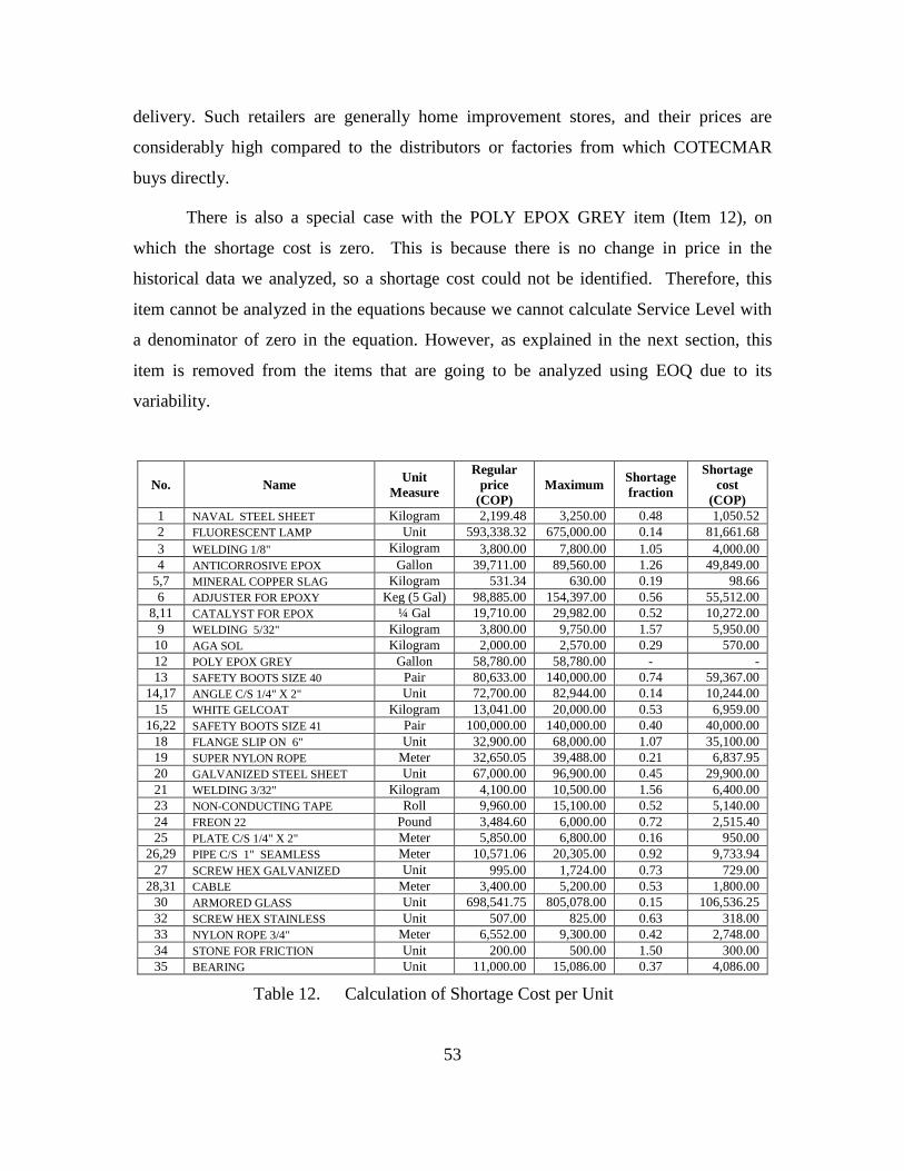
53
delivery. Such retailers are generally home improvement stores, and their prices are
considerably high compared to the distributors or factories from which COTECMAR
buys directly.
There is also a special case with the POLY EPOX GREY item (Item 12), on
which the shortage cost is zero. This is because there is no change in price in the
historical data we analyzed, so a shortage cost could not be identified. Therefore, this
item cannot be analyzed in the equations because we cannot calculate Service Level with
a denominator of zero in the equation. However, as explained in the next section, this
item is removed from the items that are going to be analyzed using EOQ due to its
variability.
No. Name Unit Measure
Regular price
(COP) Maximum Shortage
fraction
Shortage cost
(COP) 1 NAVAL STEEL SHEET Kilogram 2,199.48 3,250.00 0.48 1,050.52 2 FLUORESCENT LAMP Unit 593,338.32 675,000.00 0.14 81,661.68 3 WELDING 1/8" Kilogram 3,800.00 7,800.00 1.05 4,000.00 4 ANTICORROSIVE EPOX Gallon 39,711.00 89,560.00 1.26 49,849.00
5,7 MINERAL COPPER SLAG Kilogram 531.34 630.00 0.19 98.66 6 ADJUSTER FOR EPOXY Keg (5 Gal) 98,885.00 154,397.00 0.56 55,512.00
8,11 CATALYST FOR EPOX ¼ Gal 19,710.00 29,982.00 0.52 10,272.00 9 WELDING 5/32" Kilogram 3,800.00 9,750.00 1.57 5,950.00
10 AGA SOL Kilogram 2,000.00 2,570.00 0.29 570.00 12 POLY EPOX GREY Gallon 58,780.00 58,780.00 - - 13 SAFETY BOOTS SIZE 40 Pair 80,633.00 140,000.00 0.74 59,367.00
14,17 ANGLE C/S 1/4" X 2" Unit 72,700.00 82,944.00 0.14 10,244.00 15 WHITE GELCOAT Kilogram 13,041.00 20,000.00 0.53 6,959.00
16,22 SAFETY BOOTS SIZE 41 Pair 100,000.00 140,000.00 0.40 40,000.00 18 FLANGE SLIP ON 6" Unit 32,900.00 68,000.00 1.07 35,100.00 19 SUPER NYLON ROPE Meter 32,650.05 39,488.00 0.21 6,837.95 20 GALVANIZED STEEL SHEET Unit 67,000.00 96,900.00 0.45 29,900.00 21 WELDING 3/32" Kilogram 4,100.00 10,500.00 1.56 6,400.00 23 NON-CONDUCTING TAPE Roll 9,960.00 15,100.00 0.52 5,140.00 24 FREON 22 Pound 3,484.60 6,000.00 0.72 2,515.40 25 PLATE C/S 1/4" X 2" Meter 5,850.00 6,800.00 0.16 950.00
26,29 PIPE C/S 1" SEAMLESS Meter 10,571.06 20,305.00 0.92 9,733.94 27 SCREW HEX GALVANIZED Unit 995.00 1,724.00 0.73 729.00
28,31 CABLE Meter 3,400.00 5,200.00 0.53 1,800.00 30 ARMORED GLASS Unit 698,541.75 805,078.00 0.15 106,536.25 32 SCREW HEX STAINLESS Unit 507.00 825.00 0.63 318.00 33 NYLON ROPE 3/4" Meter 6,552.00 9,300.00 0.42 2,748.00 34 STONE FOR FRICTION Unit 200.00 500.00 1.50 300.00 35 BEARING Unit 11,000.00 15,086.00 0.37 4,086.00
Table 12. Calculation of Shortage Cost per Unit

54
In the previous section, we determined the needed variables and their values to be
used in the inventory strategy equations. In the next sections, we determine the equation
to be used according to each class of inventory, and depending on the assumptions and
rules for each approach.
C. INVENTORY MANAGEMENT FOR INDEPENDENT DEMAND ITEMS
This section contains the definition of the equations and the analysis of the
assumptions, requirements, and rules for each equation. These equations are the
Economic Order Quantity, the Service Level, and the Reorder Point.
1. Economic Order Quantity Equation Definition
The basic EOQ equation explained in Chapter II has some assumptions that must
be met to be valid. Some of the assumptions are violated by COTECMAR, according to
the data we have; thus, it is necessary to analyze each assumption and determine how to
relax it. The assumptions and their analysis are explained as follows:
• The demand is given in the form of a planning horizon to be satisfied. This is when the parts that are needed are known in advance for a specific period and their orders are planned accordingly. Conversely, at the shipyard the demand is identified on a short-term basis once a sale is done, and cannot be given in the form of a planning horizon. However, this situation is addressed with the determination of safety stocks.
• The demand is known. The demand is not known because item requirements are identified once starting repair operations. This situation is also addressed with the determination of safety stocks.
• The requirements must be satisfied at the beginning of the period. Even if it is preferable that the required items are obtained at the beginning of the period (before starting repair operations), this is not a constraint because items can be received during the operation.
• The replenishment lead time is known with certainty. Although the suppliers have regular lead times, there is some variability due to multiple factors such as: transportation delays, stockouts at the supplier, or uncontrollable situations. However, this situation is also addressed with the determination of safety stocks.
55
• The entire order quantity is delivered at the same time. In fact, partial deliveries do occur on occasion; however, because this situation occurs rarely, we assume that entire order quantities are delivered at the same time.
To relax these assumptions, an approach explained by Silver, Pyke, and Peterson
(1998) to deal with items that have time varying demand is to use the basic EOQ. This is
when there is a low variability pattern of the demand.
a. Continuous vs. Periodic Review
There are two approaches to inventory review that we can use in inventory
management strategies: continuous or periodic review. For COTECMAR, we use
continuous review because replenishment decisions are made at any moment with the
updated status of the items, using the ERP software. Periodic review happens for
consignment inventories, where, according to the consignment agreements, there is a
monthly review between the consignor and the consignee in order to quantify the
consumed items and the new replenishment requirements. However, in the case of a
stockout, COTECMAR may ask the consignor to replenish at any time, or they may
conduct a purchase with any other supplier without having to wait for the next review
period.
This project only focuses on continuous review, because we want to seek
inventory strategies with suppliers that COTECMAR does not have agreements with.
Furthermore, it is more frequent that a stockout of an item occurs if it is not in a
consignment inventory.
b. Model Selection
After seeing and analyzing the data for COTECMAR, we realize that the
shipbuilding industry is unique, in the sense that its demand and lead times are much
more complicated than many other industries. The demands do not follow a certain
pattern or a normal distribution, making it especially challenging to apply a specific
method to it.

56
According to this uniqueness, we need to identify the portion of data to
which the EOQ models can be applied. In the demand section, we have removed the
quantities that belong to special projects because those are dependent demand quantities.
However, the independent demand has some characteristics that make it difficult for the
models to be used. Therefore, we proceed by removing those quantities of demand, as
well as entire items that are still special cases. These special cases and special items may
be treated individually.
First, we refine our demand data by identifying those peak demand
quantities that go substantially out of the normal range. We suggest using those peak
quantities as special cases that might have special replenishment decisions. Therefore, we
remove the outliers in each item. This is done using the same method explained in the
lead time section. Outliers are removed from the demand data to make sure that out-of-
the-ordinary circumstances that rarely happen do not have a severe impact on our order
quantities. In this case, substantially high quantities are to be treated outside of the EOQ
calculation, and should be ordered upon request.
After refining the demand data, we proceed to calculate the coefficient of
variation. The coefficient of variation will be the factor used in deciding the approach to
determine the order quantities. In consideration of the kind of distribution of our
demand, we suggest that if the coefficient of variation is 1 or below, the basic EOQ
model is used. On the other hand, if the coefficient of variation is larger than 1, then
these items should be considered as special items and analyzed separately by
management, based on the unique case of each item.
These special items discussed above may be characterized as having long
periods without demand and scattered demand occurrences. Another characteristic is an
extremely high variation with no pattern. Figures 9 and 10 show time-series diagrams of
a couple of special items. Galvanized Steel Item has a CV of 3.63 and Flange item has a
CV of 2.58. These figures show the unique behavior of demand over time.
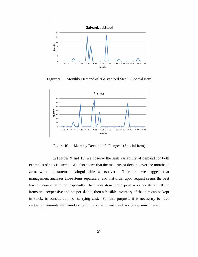
57
Figure 9. Monthly Demand of “Galvanized Steel” (Special Item)
Figure 10. Monthly Demand of “Flanges” (Special Item)
In Figures 9 and 10, we observe the high variability of demand for both
examples of special items. We also notice that the majority of demand over the months is
zero, with no patterns distinguishable whatsoever. Therefore, we suggest that
management analyzes those items separately, and that order upon request seems the best
feasible course of action, especially when those items are expensive or perishable. If the
items are inexpensive and not perishable, then a feasible inventory of the item can be kept
in stock, in consideration of carrying cost. For this purpose, it is necessary to have
certain agreements with vendors to minimize lead times and risk on replenishments.
0
5
10
15
20
25
30
1 3 5 7 9 11 13 15 17 19 21 23 25 27 29 31 33 35 37 39 41 43 45 47 49
Qua
ntity
Months
Galvanized Steel
0
10
20
30
40
50
60
70
1 3 5 7 9 11 13 15 17 19 21 23 25 27 29 31 33 35 37 39 41 43 45 47 49
Qua
ntity
Months
Flange

58
Twenty of the items were categorized as special items5, like the examples
in Figures 9 and 10. The list of these items is shown in Table 13. In this table, we show
the average monthly demand, standard deviation, and the coefficient of variation. We do
not use the EOQ on these items for the reasons mentioned earlier.
No. ITEM WAREHOUSE AVERAGE STDEV CV 2 FLUORESCENT LAMP Bocagrande 0.57 2.30 4.03 5 MINERAL COPPER SLAG Mamonal - - - 12 POLY EPOX GREY Bocagrande 7.02 22.71 3.23 14 ANGLE C/S 1/4" X 2" Mamonal 2.05 2.80 1.37 15 WHITE GELCOAT Mamonal 18.88 24.08 1.28 17 ANGLE C/S 1/4" X 2" Bocagrande 3.62 4.90 1.35 18 FLANGE SLIP ON 6" Mamonal 6.51 16.77 2.58 19 SUPER NYLON ROPE Mamonal 21.33 41.07 1.93 20 GALVANIZED STEEL SHEET Mamonal 1.57 5.70 3.63 24 FREON 22 Bocagrande 36.77 42.26 1.15 25 PLATE C/S 1/4" X 2" Mamonal 43.88 94.85 2.16 26 PIPE C/S 1" SEAMLESS Bocagrande 11.16 27.34 2.45 27 SCREW HEX GALVANIZED Bocagrande 7.59 33.73 4.44 28 CABLE Mamonal 19.39 79.59 4.11 29 PIPE C/S 1" SEAMLESS Mamonal 9.95 18.13 1.82 30 ARMORED GLASS Mamonal 0.02 0.14 7.00 31 CABLE Bocagrande 11.94 26.77 2.24 32 SCREW HEX STAINLESS Mamonal 3.27 10.85 3.32 33 NYLON ROPE 3/4" Mamonal 1.10 5.43 4.93 35 BEARING Bocagrande 0.80 1.07 1.33
Table 13. List of Special Items
In Table 14, we show the list of items that the basic EOQ model is going
to be used for. This table also contains the average monthly demand, standard deviation,
and the coefficient of variation. These independent demand items with regular quantity
ranges may be characterized by their regular demand occurrences. Furthermore, their
coefficient of variation are 1 or below. Figures 11 and 12 show time series diagrams for
two of these regular items. These figures show a normal behavior of demand over time,
even when variability is present.
5 Special Items refers to Items with very high variation (Coefficient of Variation > 1)

59
No. ITEM WAREHOUSE AVERAGE STDEV CV 1 NAVAL STEEL SHEET Mamonal 8,441.64 8,720.79 1.00 3 WELDING 1/8" Mamonal 1,241.61 836.04 0.67 4 ANTICORROSIVE EPOX Mamonal 75.79 52.83 0.70 6 ADJUSTER FOR EPOXY Mamonal 22.34 9.22 0.41 7 MINERAL COPPER SLAG Bocagrande 13,207.75 13,631.47 1.00 8 CATALYST FOR EPOX Mamonal 100.67 61.21 0.61 9 WELDING 5/32" Mamonal 776.40 604.53 0.78 10 AGA SOL Mamonal 1,547.76 1,001.81 0.65 11 CATALYST FOR EPOX Bocagrande 49.89 32.57 0.65 13 SAFETY BOOTS SIZE 40 Mamonal 11.41 8.74 0.77 16 SAFETY BOOTS SIZE 41 Mamonal 9.35 7.39 0.79 21 WELDING 3/32" Bocagrande 16.07 15.73 0.98 22 SAFETY BOOTS SIZE 41 Bocagrande 7.37 6.26 0.85 23 NON-CONDUCTING TAPE Mamonal 14.83 14.51 0.98 34 STONE FOR FRICTION Mamonal 15.80 15.84 1.00
Table 14. List of Independent Demand Items with Regular Quantity Ranges
Figure 11. Monthly Demand of “Adjuster” (Regular Item)
05
101520253035404550
1 3 5 7 9 11 13 15 17 19 21 23 25 27 29 31 33 35 37 39 41 43 45 47 49
Qua
ntity
Months
Adjuster

60
Figure 12. Monthly Demand of “Catalyst Mamonal” (Regular Item)
One important consideration in the analysis of these regular items is the
ABC classification of the items and the different approaches to be used. The different
approaches and derivations of the EOQ model used in each of the categories depend on
some characteristics inherent to each item. Such characteristics might be: dollar usage,
criticality of the item, volume, traceability, frequency, and scheduling, among many other
characteristics. As our research progressed, the uniqueness of the shipyard industry
became apparent to us. After refining the data and determining the portion of data that
the inventory management models could be applied to, we found that most of the items
lost their main characteristics. Therefore, the group of fifteen items are refined enough to
share similar characteristics, making the distinctions used in the ABC categorization no
longer applicable.
We used the ABC classification for items earlier in the project in Table 7
(Listing of Sample SKUs by Descending COP value); however, after removing the
dependent demand of all of the items, they have lost some of the characteristics including
much of the volume that drove the annual COP usage. Therefore, we now treat the items
as if all are B and C items, and use the basic EOQ, SL, and RP models presented
previously for B and C items. However, the ABC categorization may still be useful for
management decisions that deal with special items that are out of the research scope. The
following basic EOQ equation is used for items with relatively low variability:
0
50
100
150
200
250
300
1 3 5 7 9 11 13 15 17 19 21 23 25 27 29 31 33 35 37 39 41 43 45 47 49
Qua
ntity
Months
Catalyst MA

61
c. Application
Table 15 shows the economic order quantity and the variables needed to
calculate it. For example, for the EOQ calculation of Naval Steel (which is measured in
kilograms), we take the values as follows: annual demand of 101,300 kilograms, fixed
order cost of COP 235, and holding cost per unit per year of COP 115. We apply the
values into the equation:
No. Name Unit Measure WH
Annual Demand
(D)
Fixed Cost per Order (COP) (A)
Holding Cost
(COP) (r) EOQ
1 NAVAL STEEL SHEET Kilogram MA 101,300 235 115 643 3 WELDING 1/8" Kilogram MA 14,899 235 232 174 4 ANTICORROSIVE EPOX Gallon MA 909 235 2,439 13 6 ADJUSTER FOR EPOXY Keg (5 Gal) MA 268 235 6,179 5 7 MINERAL COPPER SLAG Kilogram BG 158,493 235 32 1,520 8 CATALYST FOR EPOX ¼ Gal. MA 1,208 235 1,197 22 9 WELDING 5/32" Kilogram MA 9,317 235 232 137 10 AGA SOL Kilogram MA 18,573 235 119 271 11 CATALYST FOR EPOX ¼ Gal. BG 599 235 1,197 15 13 SAFETY BOOTS SIZE 40 Pair MA 137 235 4,818 4 16 SAFETY BOOTS SIZE 41 Pair MA 112 235 4,957 3 21 WELDING 3/32" Kilogram BG 193 235 259 19 22 SAFETY BOOTS SIZE 41 Pair BG 88 235 4,957 3
23 NON-CONDUCTING TAPE
Roll MA 178 235 564 12
34 STONE FOR FRICTION Unit MA 190 235 15 76
Table 15. Economic Order Quantity (EOQ)
After separating special items from regular ones, and applying the basic
EOQ model to regular items, we can then move on to the determination of the service
level and the reorder point.
2ADEOQvr
=
2(101,300)(235)115
EOQ =
643EOQ =

62
2. Service Level
Once we determine how to calculate optimal quantities we can use the approach
described by Coleman (2000), and discussed earlier in the literature review chapter, to
figure out the correct service level. This calculation, shown below, uses holding cost,
shortage cost, and the average annual demand and economic order quantities, all—of
which have been determined in the previous section.
Service Level = 1 - (Holding Cost per Unit per Year) (Order Quantity) (Shortage Cost per Unit) (Average Annual Demand)
Table 16 shows the service level and the variables needed to calculate it. For
example, for the SL calculation of Naval Steel (which is measured in kilograms), we take
the values as follows: annual demand of 101,300 kilograms, holding cost per unit per
year of COP 115, shortage cost per unit of COP 1,051 and the calculated EOQ of 643.
We apply the values into the equation:
(115)(643)1 99.93%(1,051)(101,300)
− =

63
No. Name Unit Measure WH Annual Demand
Holding Cost (COP)
Shortage Cost (COP) EOQ SL
1 NAVAL STEEL SHEET Kilogram MA 101,300 115 1,051 643 0.9993 3 WELDING 1/8" Kilogram MA 14,899 232 4,000 174 0.9993 4 ANTICORROSIVE EPOX Gallon MA 909 2,439 49,849 13 0.9993 6 ADJUSTER FOR EPOXY Keg (5 Gal) MA 268 6,179 55,512 5 0.9981 7 MINERAL COPPER SLAG Kilogram BG 158,493 32 99 1,520 0.9969 8 CATALYST FOR EPOX ¼ Gal. MA 1,208 1,197 10,272 22 0.9979 9 WELDING 5/32" Kilogram MA 9,317 232 5,950 137 0.9994
10 AGA SOL Kilogram MA 18,573 119 570 271 0.9970 11 CATALYST FOR EPOX
¼ Gal. BG 599 1,197 10,272 15 0.9970
13 SAFETY BOOTS SIZE 40 Pair MA 137 4,818 59,367 4 0.9978 16 SAFETY BOOTS SIZE 41 Pair MA 112 4,957 40,000 3 0.9964 21 WELDING 3/32"
Kilogram BG 193 259 6,400 19 0.9961
22 SAFETY BOOTS SIZE 41 Pair BG 88 4,957 40,000 3 0.9959 23 NON-CONDUCTING TAPE Roll MA 178 564 5,140 12 0.9925 34 STONE FOR FRICTION Unit MA 190 15 300 76 0.9794
Table 16. Service Level (SL)

64
3. Reorder Point
After determining service level, the reorder point can be calculated by using the
basic method of Silver, Pyke and Peterson (1998) discussed in the literature review
chapter. Because we have refined the demand data, and separated the dependent demand
items and special quantity cases, we come up with a coefficient of variation less than or
equal to one. Therefore, we assume normal distribution for lead time and demand. The
equation to be used is as follows:
s = xL̄ + kσdLT
Table 17 shows the reorder point and the variables needed to calculate it. For
example, for the ROP calculation of Naval Steel (which is measured in kilograms), we
take the values as follows: daily demand of 281.39 kilograms, lead time demand standard
deviation of 1,592, average lead time of 7 days, lead time standard deviation of 6 days,
and a safety factor of 3.196. The lead time demand standard deviation is calculated by
scaling the monthly demand standard deviation as follows:
The safety factor is calculated using the excel function NORMSINV of the service level
calculated above. Finally, we calculate:
For example, for Naval Steel we apply the values into the equation as follows:
1( )*30
DailySTDEV MonthlySTDEV=
2 2 2( * ) (( ) * )dLT d LTAverageLT AverageDailyDemandσ σ σ= +
2 2 2(281.39)(7) (3.196)( (7*1,592 ) (281.39 *6 )) 15,960+ + =

65
No. Name Unit Measure WH
Daily Demand
(x̄L)
Daily Demand
Stdev (σD)
Average lead time (LT)
lead time Stdev (σLT)
Safety Factor
(k) SL ROP
1 NAVAL STEEL SHEET Kilogram MA 281.39 1,592 7 6 3.196 0.9993 15,960 3 WELDING 1/8" Kilogram MA 41.39 153 3 3 3.204 0.9993 1,056 4 ANTICORROSIVE EPOX Gallon MA 2.53 10 6 4 3.189 0.9993 97 6 ADJUSTER FOR EPOXY Keg (5 Gal) MA 0.74 2 6 3 2.898 0.9981 18 7 MINERAL COPPER SLAG Kilogram BG 440.26 2,489 29 30 2.733 0.9969 64,528 8 CATALYST FOR EPOX ¼ Gal. MA 3.36 11 6 4 2.862 0.9979 109 9 WELDING 5/32" Kilogram MA 25.88 110 3 3 3.251 0.9994 713
10 AGA SOL Kilogram MA 51.59 183 3 3 2.743 0.9970 1,183 11 CATALYST FOR EPOX ¼ Gal. BG 1.66 6 6 4 2.749 0.9970 55 13 SAFETY BOOTS SIZE 40 Pair MA 0.38 2 22 20 2.853 0.9978 39 16 SAFETY BOOTS SIZE 41 Pair MA 0.31 1 23 20 2.687 0.9964 31 21 WELDING 3/32" Kilogram BG 0.54 3 2 1 2.658 0.9961 14 22 SAFETY BOOTS SIZE 41 Pair BG 0.25 1 23 20 2.647 0.9959 25 23 NON-CONDUCTING TAPE Roll MA 0.49 3 5 4 2.432 0.9925 18 34 STONE FOR FRICTION Unit MA 0.53 3 6 5 2.041 0.9794 20
Table 17. Reorder Point (ROP)

66
D. FINDINGS
We begin our findings with a table summarizing the items analysis. Then, we
categorize our findings using Demand, Price, Item, Lead Time, and Process Issues. The
following are the findings.
1. Summary Table
Table 18 is a summary table explaining the transition that led us from our 35
sample items to the 15 items analyzed using the EOQ model. First, we took the total
annual demand quantity and separated out the dependent demand quantities that belong to
known-in-advance projects such as shipbuilding and overhauling. For these quantities we
recommend to use MRP approach. The remaining quantities are independent demand
items. We calculated the coefficient of variation (CV) to determine the suitable inventory
management approach. For items with high variability (CV>1), we recommended
separate analysis by management. For example, items with large CV typically have zero
demand in most time periods and positive demand in only a few time periods. Thus, the
management should try to determine the drivers of demand, i.e. what caused the positive
demand. With this analysis in place, the management is in a position to better plan for
the inventory of these items with high CV. The remaining 15 items are independent
demand items with CV lower than 1. For these items, we recommended using the basic
EOQ approach.

67
No. Name WH Total
Annual Demand Q
Dependent Demand Q
Appropriate Method for Dependent Quantity
Independent Demand Q CV
Appropriate Method for
Independent Quantity
1 NAVAL STEEL SHEET MA 252,863.25 151,563.59 MRP 101,299.66 1.00 EOQ Model 2 FLUORESCENT LAMP BG 278.67 271.81 MRP 6.86 4.03 Separate Analysis 3 WELDING 1/8" MA 31,358.50 16,459.15 MRP 14,899.35 0.67 EOQ Model 4 ANTICORROSIVE EPOX MA 2,613.75 1,704.30 MRP 909.45 0.70 EOQ Model 5 MINERAL COPPER SLAG MA 165,890.00 165,890.00 MRP - 0.00 Separate Analysis 6 ADJUSTER FOR EPOXY MA 778.75 510.66 MRP 268.09 0.41 EOQ Model 7 MINERAL COPPER SLAG BG 158,493.00 26,415.50 MRP 132,077.50 1.00 EOQ Model 8 CATALYST FOR EPOX MA 3,541.13 2,333.08 MRP 1,208.04 0.61 EOQ Model 9 WELDING 5/32" MA 17,812.50 8,495.75 MRP 9,316.75 0.78 EOQ Model
10 AGA SOL MA 31,106.88 12,533.76 MRP 18,573.11 0.65 EOQ Model 11 CATALYST FOR EPOX BG 2,502.50 1,903.78 MRP 598.72 0.65 EOQ Model 12 POLY EPOX GREY BG 534.50 450.26 MRP 84.24 3.23 Separate Analysis 13 SAFETY BOOTS SIZE 40 MA 239.00 102.04 MRP 136.96 0.77 EOQ Model 14 ANGLE C/S 1/4" X 2" MA 288.75 264.20 MRP 24.55 1.37 Separate Analysis 15 WHITE GELCOAT MA 1,070.50 844.00 MRP 226.50 1.28 Separate Analysis 16 SAFETY BOOTS SIZE 41 MA 179.75 67.58 MRP 112.17 0.79 EOQ Model 17 ANGLE C/S 1/4" X 2" BG 236.25 192.85 MRP 43.40 1.35 Separate Analysis 18 FLANGE SLIP ON 6" MA 252.25 174.13 MRP 78.12 2.58 Separate Analysis 19 SUPER NYLON ROPE MA 298.75 42.83 MRP 255.92 1.93 Separate Analysis 20 GALVANIZED STEEL SHEET MA 156.50 137.64 MRP 18.86 3.63 Separate Analysis 21 WELDING 3/32" BG 1,968.50 1,775.72 MRP 192.78 0.98 EOQ Model 22 SAFETY BOOTS SIZE 41 BG 88.50 0.09 MRP 88.41 0.85 EOQ Model 23 NON-CONDUCTING TAPE MA 682.75 504.79 MRP 177.96 0.98 EOQ Model 24 FREON 22 BG 1,730.25 1,289.00 MRP 441.25 1.15 Separate Analysis 25 PLATE C/S 1/4" X 2" MA 1,037.25 510.72 MRP 526.53 2.16 Separate Analysis 26 PIPE C/S 1" SEAMLESS BG 491.74 357.81 MRP 133.92 2.45 Separate Analysis 27 SCREW HEX GALVANIZED BG 6,382.50 6,291.40 MRP 91.10 4.44 Separate Analysis 28 CABLE MA 1,397.25 1,164.60 MRP 232.65 4.11 Separate Analysis 29 PIPE C/S 1" SEAMLESS MA 429.42 310.08 MRP 119.35 1.82 Separate Analysis 30 ARMORED GLASS MA 2.50 2.26 MRP 0.24 7.00 Separate Analysis

68
31 CABLE BG 451.25 307.98 MRP 143.27 2.24 Separate Analysis 32 SCREW HEX STAINLESS MA 1,614.25 1,575.07 MRP 39.18 3.32 Separate Analysis 33 NYLON ROPE 3/4" MA 52.00 38.78 MRP 13.22 4.93 Separate Analysis 34 STONE FOR FRICTION MA 1,280.25 1,090.70 MRP 189.55 1.00 EOQ Model 35 BEARING BG 31.50 21.85 MRP 9.65 1.33 Separate Analysis
Table 18. Items Analysis Summary

69
2. Demand Issues
There is much variation in the demand across different years. Some variation is
caused by the distinctiveness of vessels (which require different items), and even if they
require the same kind of items, they might require different models. Another reason for
this variation is that some projects (like shipbuilding and overhauling) last more than two
years, or span different periods; this leads to demand being governed by the schedule of
the project. For instance, an overhauling project of changing engines and fresh water
system for a vessel may be divided across years. So, the demand for engine spares and
equipment may be scheduled this year and the demand for fresh water pumps may be
scheduled next year. This causes a disproportionate demand from one year to another.
There are some specific items that are needed for a specific vessel or project, and
then, not needed again for a while. For instance, submarine spare parts are only required
once every several years in COTECMAR; but when they are required, they are required
in high quantities with some urgency.
Due to technology advancements or the practicality of an item, the demand of
some items grows significantly over the years and the demand of others decreases
significantly over the years. Therefore, this will affect the average demand and make it
harder to make good forecasts of demand.
3. Price Issues
There is variation in the prices without any constant pattern. There is no regular
increase over time; instead, sometimes the prices go down due to negotiation.
Some outlier prices have an effect on the average price. Most of these outlier
prices are due to a sudden change of supplier for reasons like urgent need, or stockout of
the regular supplier. Other outlier prices are created by typos. These kinds of typos are
easy to check because such values are surprisingly high, and we can see how the same
supplier offered us the regular correct price on very close dates.

70
There is lack of data for certain items in some POs, because they are supplier
consignments. Thus, most of the information, such as average price, is based only on
warehouse transactions.
4. Item Issues
Some items are sold in different packaging (one liter or half liter), but this
condition (which makes them different SKUs) does not affect the usage for production
purposes. For example, the item CATALYST FOR POLY EPOX comes in two different
packages. One comes in a ¼ gallon container and the other comes in a 1/8 gallon
container. Therefore, we need to take into account both packages in order to get a unified
demand in gallons.
5. Lead Time Issues
The standard deviation of the lead time is high in some items because of outlier
cases that happen every once in a while. Lead times for the same items are mostly close
to each other; however, in rare instances there is a drastic change in lead times due to
extraordinary events.
There is lack of information for some items, especially in the receiving dates of
the inventory. Sometimes the same items have no receiving dates in some purchase
orders, and have a receiving date on other purchasing orders. This is caused by
consignments that are signed with vendors where they have items in COTECMAR’s
warehouse, which makes the lead time zero. In some instances, vendors are out of that
item, which necessitates ordering more from other suppliers. This creates a non-zero
lead time.
6. Process Issues
In the Warehouse Transaction file, we find that the warehouse employees, instead
of registering returns from investment and administrative projects with the correct
transaction code (RS), they type negative deliveries. This means that there is no standard
process for the same transaction even when they come from different projects.

71
We find many returns by the projects in the data. In some cases, the projects
return the complete quantity or more than half of what they asked for. Sometimes, they
do so in order to have extra stocks during the works, to avoid delay in case they need
more. Sometimes it is due to lack of planning or inaccurate calculation of their needs.
This situation may create unnecessary stockouts, and fake alerts of replenishment needs.
E. SUMMARY
This chapter covered the determination of the needed variables for inventory
management calculations. We calculated annual demand and separated the dependent and
independent demand items quantities. We calculated order lead times and refined the data
from outliers. Then we calculate holding cost per unit, fixed cost per order and shortage
cost per unit.
This chapter included discussion of different inventory models, along with the
assumptions related to each one and the selection of the basic EOQ model for
independent demand items quantities that have CV equal or lower than one.
Furthermore, in this chapter, we apply the data of the selected items in all of the
equations. Finally, all of the findings are listed. In the following chapter, working from
these calculations and findings, we present conclusions, recommendations for
management, and suggestions for future research.

72
V. CONCLUSIONS AND RECOMMENDATIONS
This chapter is presented in three parts. The first part contains our conclusions,
the second part presents our recommendations for management, and the last part contains
our suggestions for future research.
A. CONCLUSIONS
We categorize our conclusions into demand, lead time, general inventory
management issues, and calculation results. The following are the conclusions.
1. Demand Conclusions
Based on the demand data, we find that about 40% of the inventory is
independent demand items. The remaining 60% of the inventory is dependent demand
items that must be treated using processes such as MRP. This is a normal circumstance
for an industry (like a shipyard) that performs different business functions, where a big
portion of their business comes from planned projects such as shipbuilding or
overhauling in which replenishments can be planned in advance. The 40%, that are
independent demand items, come from business functions like ship repair and
maintenance. Here the demand is not known in advance and EOQ models may be
applicable. However, even when we may apply any strategy to a certain portion of the
demand, there is a need for a suitable inventory strategy for the other portion of the
demand as well.
We conclude that a major portion of COTECMAR demand, which is dependent,
may be managed with some approaches such as the MRP described in this project.
However, the Bill of Materials list, from an MRP approach, will vary from project to
project. This is true even when ships are to be built with the same general specifications.
This happens due to constant technology improvement and differences in customer
requirements. Furthermore, item demands resulting from overhaul projects are
completely different depending on which vessel the shipyard is working on.

73
2. Lead Time Conclusions
We find in the lead time data that there are some outliers that greatly affect the
lead time average, and especially the standard deviation of the errors of forecasts.
Although the outlier lead time is a reality in every corporation, taking account of it affects
both the service level and the decisions about when and how much replenishment is
required, thus distorting the calculations. One example is when production employees
send a request directly to the supplier instead of following the regular channel. Once the
item arrives at the warehouse, the warehouse does not accept it because there is no
purchase order. This leads to all the paper work being done in one day. This gives such
items a specific lead time of zero or one day, thus distorting the actual lead time.
Another example is the case in which a supplier experiences unusual
circumstances, like a sudden stockout and in which they must ask for an extension in the
delivery time, thus distorting the actual lead time. In this case, the purchasing division
buys from any other supplier, giving continuity to replenishment. These are both
examples of unique situations that do not have to affect decisions based on lead times,
because they do not happen under normal situations.
3. Inventory Management Conclusions
In the beginning of the literature review we explained two known classification
models. These models are analyzed in order to see if they are suitable or applicable to the
shipyard. We find that Kraljic model is useful when there are purchasing portfolio
decisions to be made. ABC model is useful for simple inventory management models
using EOQ. However, after our research progressed and after analyzing the findings, we
conclude that the Kraljic and the ABC models are not suitable for COTECMAR’s
inventory management. Instead, a more suitable approach is to classify items by whether
they are Dependent- or Independent-demand items, and to use EOQ approach for items
with low coefficient of variation in demand.
It is necessary to determine a strategy that might be suitable for all of the items
regardless of the final user in order to standardize the purchasing process for items that
may be needed for regular or sporadic projects.
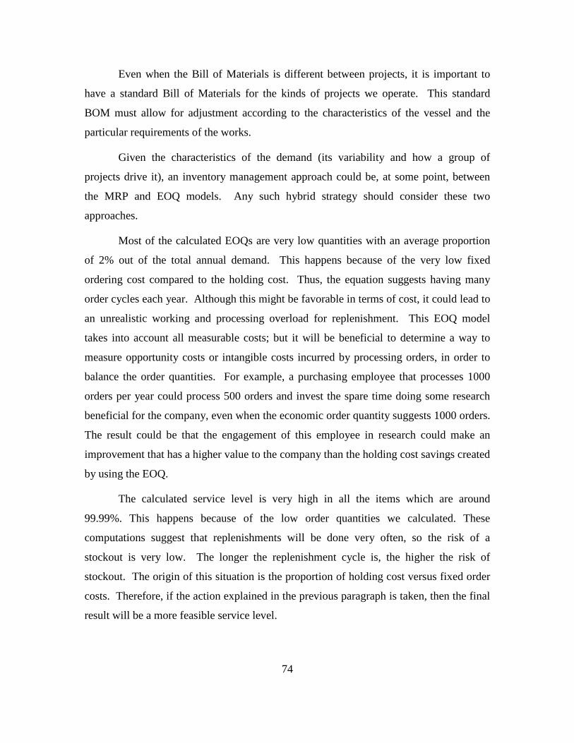
74
Even when the Bill of Materials is different between projects, it is important to
have a standard Bill of Materials for the kinds of projects we operate. This standard
BOM must allow for adjustment according to the characteristics of the vessel and the
particular requirements of the works.
Given the characteristics of the demand (its variability and how a group of
projects drive it), an inventory management approach could be, at some point, between
the MRP and EOQ models. Any such hybrid strategy should consider these two
approaches.
Most of the calculated EOQs are very low quantities with an average proportion
of 2% out of the total annual demand. This happens because of the very low fixed
ordering cost compared to the holding cost. Thus, the equation suggests having many
order cycles each year. Although this might be favorable in terms of cost, it could lead to
an unrealistic working and processing overload for replenishment. This EOQ model
takes into account all measurable costs; but it will be beneficial to determine a way to
measure opportunity costs or intangible costs incurred by processing orders, in order to
balance the order quantities. For example, a purchasing employee that processes 1000
orders per year could process 500 orders and invest the spare time doing some research
beneficial for the company, even when the economic order quantity suggests 1000 orders.
The result could be that the engagement of this employee in research could make an
improvement that has a higher value to the company than the holding cost savings created
by using the EOQ.
The calculated service level is very high in all the items which are around
99.99%. This happens because of the low order quantities we calculated. These
computations suggest that replenishments will be done very often, so the risk of a
stockout is very low. The longer the replenishment cycle is, the higher the risk of
stockout. The origin of this situation is the proportion of holding cost versus fixed order
costs. Therefore, if the action explained in the previous paragraph is taken, then the final
result will be a more feasible service level.

75
The calculated reorder point is also very high for all of the items. This is driven
by high variability of demand and lead time, and the extremely high service level. We
can see that, from the beginning of our calculation, we observe low EOQs which had a
direct effect on the service levels and the order points. The order point calculation
suggests keeping high inventory levels—enough to cover the high variability. This has
pros and cons: the pros include decreasing the risk of stockouts; however, the cons
include high holding costs and obsolescence in some items.
4. Conclusions about Results of Calculations
The first issue we observe is that there is a problem with the calculation of the
fixed ordering cost because this low fixed ordering cost is leading to low values of EOQ
and, consequently, high values of SL and ROP. Therefore, it is important to include
opportunity ordering costs and intangible ordering costs to show not only an optimal
economic calculation, but also feasible, realistic, and manageable workload quantities
that fit in a normal replenishment process.
The second issue is the characteristic of the demand itself, due to uniqueness of
the shipyard industry, because the historical data does not provide normal standard
deviations. It is also difficult to conduct a forecast based on the historical time-series
data, due to the variability and uniqueness of each project. Therefore, it is necessary to
create a forecasting method that is not solely based on historical data, but also includes:
markets, the types of vessels of the shipyard customer, and the kind of repairs requested
by the customers or conducted by the shipyard.
B. RECOMMENDATION FOR MANAGEMENT
A suggestion for management is to improve the information-sharing process
between the shipyard and the customers, in order to make better decisions on inventory
levels and replenishment cycles. One way to improve this process is to establish one-to-
one communications between the customer ship engineers and COTECMAR engineers
that will help the shipyard to improve predictions on what items are needed for repair.
This procedure should be standardized and formalized, in order to take this information
as the replenishment input for the purchasing department. This formality creates

76
accountability and avoids over-ordering materials when they are not needed. The
shipyard could start this process with its biggest customer, the Colombian Navy. It
would be easier to start with them because COTECMAR is mainly owned by the Navy.
Once the shipyard demonstrates the benefit of this process with the Navy, it can
implement the same process with private customers. This process could deliver more
accurate and economic stock levels with high service levels.
Another suggestion to management is to continuously upgrade the information
system (ERP) in the shipyard as technology advances, so that it will be able to rely on
more effective systems that will decrease the need for keeping inventories. A good data
resource will also reduce the inaccuracy in demand calculations and forecasts. This will
help to reduce the need for safety stocks. Furthermore, agreements and relationships
between the shipyard and its suppliers should be improved. The improvement could be
sharing information on a timelier basis for making better managerial decisions. This
could lead to decreasing lead times (and lead time variability) and lowering expediting
and processing costs, which can have a significant effect on improving inventory
management. Moreover, the information should be implemented across the entire supply
chain to timely manage information about demand. This is done so suppliers can
anticipate replenishment needs without having to wait until the information goes through
the complete supply chain. This delay creates a loss of time and a bullwhip effect, which
leads to overstocks and obsolescence in materials.
After progressing in our research, we find that the shipyard industry has distinct
traits that are different from most other industries. In other industries historical data,
cases of seasonality, patterns, and drivers provide fairly accurate information about
demand, which makes applying inventory management easier. However, the shipyard
industry is completely different from the regular ones. It has thousands of items, extreme
variability of demand over time, regularly changing products due to technology
advancements, multiple systems in single ships (propulsion, furniture, hull), and different
requirements for each ship.

77
Management should look into doing more analysis into the demand requirements
based on the kind of ships coming in for repair rather than predicting demand based time.
A conclusion in this research is that demand is strongly related to the kind of ships being
repaired, without following time-based patterns. Therefore, this demand analysis could
be done by gathering historical data of the ships that have been in the shipyard. Then, the
demand for the most common types of ships can be analyzed in order to determine
similarities in the items demanded, or if there are existing patterns. This information
could be useful in order to forecast possible items that might be needed once the shipyard
knows about an upcoming ship. For this particular industry, this demand forecast could
result in more accurate results than forecasting demand based on time.
C. SUGGESTIONS FOR FUTURE RESEARCH
There are some cons and pros to using both continuous and periodic review.
Periodic review could be less expensive in terms of reviewing costs and reviewing errors.
On the other hand, under continuous review the safety stock needed to provide the same
customer service level is lower; thus, overall holding costs are less expensive. It will
beneficial to conduct a cost benefit analysis to compare these two review methods in
order to implement the optimal method in the corporation.
This project focuses on items that were under continuous review. Therefore,
future research on determining the optimal replenishment quantities for consignment
inventories would be beneficial. This kind of inventory follows a periodic review
process, but is interrupted on every stockout. An optimal quantity will allow for having
replenishments in the determined periods, and it will also avoid the violation of the
periodic review basic principle.
This project focused on items that were independent and looked into EOQ models
to manage them. Since the majority of items were dependent in this industry and EOQ
models are not applicable, it would be beneficial for other researchers to focus on
strategies to manage dependent items. This will entail more detailed research on MRP
approaches that deal with thousands of distinct items for each project, as this is normal in
shipbuilding projects.
78
This project determines demand based on time, which shows that shipyard
industries require demand of items with a high variability between different periods.
Most of this variability is driven by the characteristics of the ships rather than the
periodicity of the works on these ships. It might be beneficial in future projects to show
demand based on ships rather than time. This might lead to more accurate demand
forecasts and reduce variability of demand.
In this project, we find the parameters needed to determine service levels based on
the optimal number of stockout occasions and the number of exposures to stockout for
each item each year. However, we recommend applying these models to a larger sample
in order to determine if that is the service level desired for management.

79
LIST OF REFERENCES
Arango, M., Adarme, W., Cogollo, J., Otero, M., Hernández, J., Angulo, A. et al. (2012, January). Desarrollo de un modelo logístico que permita el incremento de la competitividad en Cotecmar. (University Faculty Project). Cartagena de Indias, Colombia: Dirección Administrativa y Financiera – Cotecmar.
Baily, P. (1987). Purchasing and supply management (5th ed.). Bristol, Great Britain: Chapman and Hall.
Caniëls, M., & Gelderman, C. (2005). Purchasing strategies in the Kraljic matrix – A power and dependence perspective. Journal of Purchasing and Supply Management,11(2-3) 141–155.
Coleman, B. (2000). Determining the correct service level target. Production and Inventory Management Journal, 41(1), 19–23. Retrieved from http://search.proquest.com/docview/199930161?accountid=12702.
Diaz, L. and Leaño, C. (2009, December). Sistema de clasificación de proveedores de Cotecmar. (Internship Project). Cartagena de Indias, Colombia: Dirección de Investigación, Desarrollo e Innovación – Cotecmar.
Ettl, M., Feigin, G., Lin, G. and Yao, D. (2000), “A supply network model with base-stock control and service requirements,” Operations Research, 28(March/April), 216–32.
Jeffery, M., Butler, R. and Malone, L. (2008). Determining a cost-effective customer service level. Supply Chain Management: An International Journal, 13(3), 225–232.
Keller, G. (2009). Statistics for management and economics (8th ed.). Mason, OH: South Western Cengage Learning.
Kraljic, P. (1983). Purchasing must become supply management. Harvard Business Review, 61(5), 109–117.
Rinehart, L., Cooper, M. and Wagenheim, G. (1989). Furthering the integration of marketing and logistics through customer service in the channel. Journal of the Academy of Marketing Science, 17(1), 63–71.
Silver, E. A., Pyke, D. F., & Peterson, R. (1998). Inventory management and production planning and scheduling (3rd ed.). New York, NY: Wiley.
Zipkin, P. (2000). Foundations of inventory management. Boston, MA: McGraw-Hill.

80
THIS PAGE INTENTIONALLY LEFT BLANK

81
INITIAL DISTRIBUTION LIST
1. Defense Technical Information Center Ft. Belvoir, Virginia
2. Dudley Knox Library Naval Postgraduate School Monterey, California
3. Professor Uday Apte
Naval Postgraduate School Monterey, California
4. Professor Susan Heath
Naval Postgraduate School Monterey, California
5. CN. Jorge Gomez Bejarano Vice-president COTECMAR Cartagena, Colombia
6. CF. Oscar Dario Tascón
DIDESI - COTECMAR Cartagena, Colombia
7. CF. Martín Orduz Rodríguez DIRFAD - COTECMAR Cartagena, Colombia
8. Brigadier Alaa Seyadi
Bahrain Coastguard Commander Ministry of Interior Manama, Bahrain


