
IAME 2016 CONFERENCE | HAMBURG
Paper ID 115
Development of a ship weather routing system
for energy efficient shipping
Tong Cui, Osman Turan, Evangelos Boulougouris
Department of Naval Architecture and Marine Engineering, University of Strathclyde,
100 Montrose Street, Glasgow G4 0LZ, UK, [email protected]
Abstract
In this paper, a new ship weather routing system is developed towards enhancing energy
efficiency. The routes searching is essentially regarded as an optimisation process with two
objectives, which are respectively ETA (estimated arrival time) and fuel consumption. When
ship characteristics, loading conditions, ship speed, and sea conditions (wave, wind and
currents) are imported to this system, together with departure and final points and departure
time, a set of minimum fuel consumption routes under different ETA can be achieved. In
this way, an optimal and safe enough route can be decided according to shipping schedule.
A combination of global and local optimisation strategy is used in weather routing
optimisation. Finally, an Aframax Oil Tanker is taken as a case study to prove the validity of
this ship weather routing decision system.
Keywords: marine transport, weather routing, energy efficiency, two objectives
optimisation
1. Introduction
In the shipping field, energy consumption is quite huge, as almost 90% goods traded
worldwide are transported by sea. With the development of marine transport and people's
enhancing awareness of energy conservation, the selection of ship routes is getting more and
more attention in the shipping industry. Especially in recent years, the global economic
recession led to a downturn in the shipping industry, improving energy saving capability of
the ship from the technical level, to minimize the cost of transportation has become a
pressing issue faced by the technician. In essentially, ship route searching can be defined as
an optimisation process, which is always affected by hull form, weather, sea states and ship
safety, etc. To save travel time, maximise safety or energy efficiency, people have
developed many kinds of optimisation methods. Most common methods are listed as below.
Development of a ship weather routing system for
energy efficient shipping
115
IAME 2016 Conference | August 23 - 26, 2016 | Hamburg, Germany 2
Calculus of variations (Bijlsma S.J, 1975) is a method that calculates the optimal heading
between two points by solving Euler equation. The optimal route can be determined by
refining the gradients of arbitrary objective function in a continuous optimisation process.
Isochrone method (James, 1957) is a very common method used in ship routing and even
much commercial software, like OpenCPN, qtVlm etc. It generates isochrones one by one
repeatedly, which means setting several lines a ship can reach after a certain time from the
departure point. From these lines, a minimum ETA route can be easily determined. It also
has some modified version (Hagiwara H, 1989, Hagiwara H & Spaans JA, 1987) for
different calculation objectives.
The principle of Isopone method (Klompstra MB et al., 1992, Spaans JA, 1995) is similar to
Isochrone method. It defines the shipping boundary with equal fuel consumption in a three-
dimensional space. This method can easily obtain minimum fuel consumption route.
Dijkstra’s method (Padhy, 2008; Panigrahi, 2008, Hege Eskild, 2014) was introduced to ship
routing recently, which is a kind of graph searching optimisation method. Before
calculation, a network was built based on grids system, and then positive weights represent
passage time or fuel consumption, etc. were assigned to the graph edges. By analysing the
sum of weights on this network, optimal route with different objectives can be determined.
Dynamic programming method is developed based on Bellman’s principle of optimality
(Bellman, 1957). The main strategy is: solving the big problem by dividing it to many sub
small problems. Results from each subproblem will form the final result. Some researchers
(De Wit C, 1990, Calvert S et al., 1991) developed a 2-dimensional dynamic programming
(2DDP) method for ship routing problem, which takes two dimensions: latitude and
longitude into account. This method simplifies the problem and reduces the calculation time.
Based on that, Wei Shao (2012) developed a 3-dimensional dynamic programming (3DDP)
method, which contains 3-dimensional variables: latitude, longitude and time and uses a
forward algorithm in the optimisation process. This method can provide better ship routing
results without increasing much calculation cost. Besides, there are also some evolutionary
algorithms, like Genetic Algorithm (Harries, 2003, Hinnenthal, 2010, and J.Szłapczy´nska,
2009).
In this paper, a ship weather routing system for energy efficient shipping is developed. This
system has relative more comprehensive functions, including grids system design, weather
data download, shipping safety testing, fuel consumption calculation and optimal route
Development of a ship weather routing system for
energy efficient shipping
115
IAME 2016 Conference | August 23 - 26, 2016 | Hamburg, Germany 3
selection etc. A combination of global and local optimisation strategy is used in weather
routing optimisation. The system runs towards to two objectives: ETA and fuel
consumption. Finally, an optimisation Pareto front can be generated, and then the optimal
route according to different shipping requirements can be determined.
2. Ship weather routing system
2.1. Preparatory work
Before calculation in the ship weather routing system, some necessary files and data should
be collected in advance. Firstly, for a certain ship, its characteristics are collected, including
ship geometry, main engine and propeller parameters. Secondly, based on Holtrop 84
(1984) resistance prediction method and strip theory, ship calm water resistance coefficient
curve and response amplitude operators for different motions can be calculated respectively.
Strip theory can also be used to define transfer functions. Next ship response in the irregular
sea can be found by combining the transfer function with the wave spectrum (JONSWAP).
Besides, added resistance due to waves, wind resistance coefficient curve and propeller open
water performance file are also calculated. Added resistance file are calculated based on the
method presented by Gerritsma and Beukelman (1972). Loukakis and Sclavounos (1978)
extended this method from only valid for head sea waves to oblique waves. This file
includes relative wave angle, mean wave period and significant height of combined wind
waves and swell, and corresponding added resistance value under these conditions. So that
when three arbitrary conditions are given, a certain added resistance value due to waves can
be got. Similarly, propeller open water performance file contains advance coefficient, thrust
coefficient, torque coefficient and open water efficiency.
2.2 Grids system design module
Grids system is designed in advance for leading the ship travel. In this grids system, great
circle (The shortest distance between two points on a sphere) is taken as the reference, which
is divided into several equal stages with certain numbers of points. Through every point, a
straight line can be drawn perpendicular to its tangent line around the circle. Next, certain
numbers of points can be distributed along this vertical line, including upper and lower parts
of the great circle. The number of stages and distance between two points in one stage are
both adjustable. The grids system can be clearly explained in Figure 1.

Development of a ship weather routing system for
energy efficient shipping
115
IAME 2016 Conference | August 23 - 26, 2016 | Hamburg, Germany 4
Figure 1 – Grids system
After the grids system is fixed, travel directions should be determined from every departure
point to arrival point. Considering the larger course deviations are not feasible and would be
unrealistic for an optimum route, five directions are better. So that, from departure point,
except points near the grids border, a ship at every point can travel to next five potential
points, which can be seen in Figure 2. With these nodes are connected, many potential arcs
are formed.
Figure 2 – Ship routing network
2.3 Files reading module
This is also the entry point to the whole weather routing system. Two file types should be
read and decoded.
Development of a ship weather routing system for
energy efficient shipping
115
IAME 2016 Conference | August 23 - 26, 2016 | Hamburg, Germany 5
First, from 2.1, based on ship characteristics, many calculation result files have been got,
including calm water resistance coefficient curve, transfer functions for different motions,
added resistance file due to waves, wind resistance coefficient curve and propeller open
water performance file. All of the files are edited to certain form in a .txt file, which will be
input to the system for weather routing calculation.
Second, weather forecast files are downloaded from different database. This system will take
winds, waves and currents into account together. For waves and winds, they are downloaded
from ECMWF (European Centre for Medium-Range Weather Forecasts) (.grib), including
10 meter U wind component, 10 meter V wind component, mean wave direction, mean
wave period and significant height of combined wind waves and swell, and they all update
every 6 hours. For currents, it is downloaded from NOAA (National Oceanic and
Atmospheric Administration) (.nc), including 15-meter depth U current component and V
current component, and updates every five days. All of these weather data files contain time,
latitude and longitude. Once time, latitude and longitude at a certain point on the earth were
given, detailed weather data at that point will be known in this module.
2.4 Ship navigation safety module
This is a very important module since it relates to the safety of ship and crew. Seakeeping
performance is introduced here to guarantee the ship navigation safety. Within this module,
four parameters are calculated according to NORDFORSK criteria (1987). They are
probability of slamming, probability of deck wetness, RMS of roll and RMS of relative
vertical acceleration. All of them should be less than corresponding criteria according to
different navigation situation. They are all calculated based on transfer functions pre-
calculated in 2.1. Seakeeping performance can be regarded as a constraint for the following
optimisation. If the sea condition of a certain area does not satisfy the ship’s navigation
requirements, a “No Entry” signal will be assigned to this area, so that the ship will not go
through this area.
2.5 Fuel consumption calculation module
In this system, only added resistance due to waves and winds are taken into account. Total
resistance can be calculated by:
Rtotal=Rcalm+Rwaves+Rwinds (1)
Among them, when a certain speed in calm water is given, Rcalm can be easily got by
interpolation with calm water resistance coefficient curve. Rwaves can be calculated by the file
“added resistance due to waves” mentioned in 2.1, with introduced waves weather data.
Development of a ship weather routing system for
energy efficient shipping
115
IAME 2016 Conference | August 23 - 26, 2016 | Hamburg, Germany 6
Similarly, according to winds weather data, Rwinds can be got by interpolation with wind
resistance coefficient curve as well.
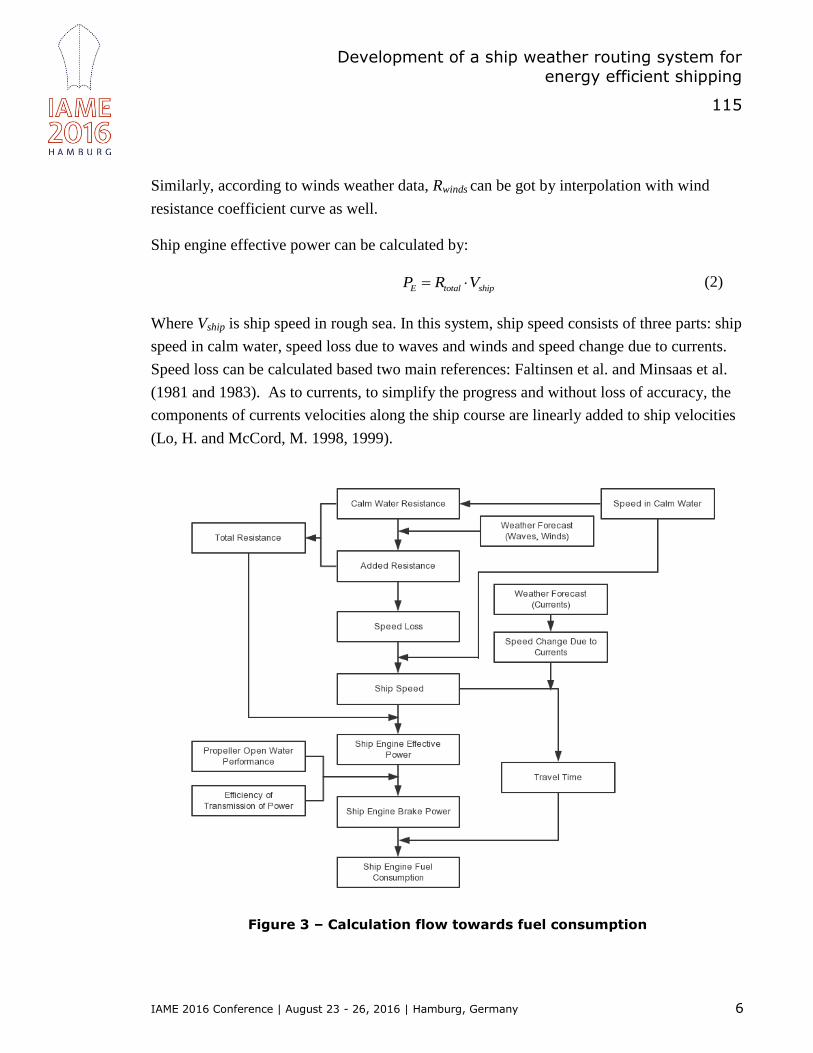
Ship engine effective power can be calculated by:
E total shipP R V (2)
Where Vship is ship speed in rough sea. In this system, ship speed consists of three parts: ship
speed in calm water, speed loss due to waves and winds and speed change due to currents.
Speed loss can be calculated based two main references: Faltinsen et al. and Minsaas et al.
(1981 and 1983). As to currents, to simplify the progress and without loss of accuracy, the
components of currents velocities along the ship course are linearly added to ship velocities
(Lo, H. and McCord, M. 1998, 1999).
Figure 3 – Calculation flow towards fuel consumption
Development of a ship weather routing system for
energy efficient shipping
115
IAME 2016 Conference | August 23 - 26, 2016 | Hamburg, Germany 7
Next, propeller characteristics and open water performance file are introduced here to
calculate the hull efficiency H , open water efficiency 0 and relative rotative efficiency R .
Together with the mechanism transmission efficiency: shaft efficiency S and gearbox
efficiencygb , the engine brake power can be determined from:
0
EB
H R S gb
PP
(3)
Finally, the fuel consumption for a certain arc can be calculated by:
BFC P sfoc t (4)
Where, sfoc (g/kWh) is specific fuel oil consumption of the engine, which is assumed as a
constant value in this system. t is ship navigation duration, which can be easily got when the
length of the arc and actual ship speed are known.
The calculation flow of ship fuel consumption for every small arc can be seen in Figure 3.
2.6 Route optimisation module
The route optimisation strategy used in this system is a combination of global and local
optimisation with two objectives: ETA and fuel consumption.
The calculation starts from the departure point. Firstly, the system reads the weather data at
the departure point by local longitude, latitude and departure time. Secondly, as can be seen
from the grids system in 2.2 and Figure 4, the whole travel route can be divided into several
stages, so that the ship can travel along the route stage by stage. Within every stage, there
are many departure points and arrival points, and almost every point (without the point near
the grids border) can go to next stage by five directions. So there are many potential route
arcs in one stage.
Development of a ship weather routing system for
energy efficient shipping
115
IAME 2016 Conference | August 23 - 26, 2016 | Hamburg, Germany 8
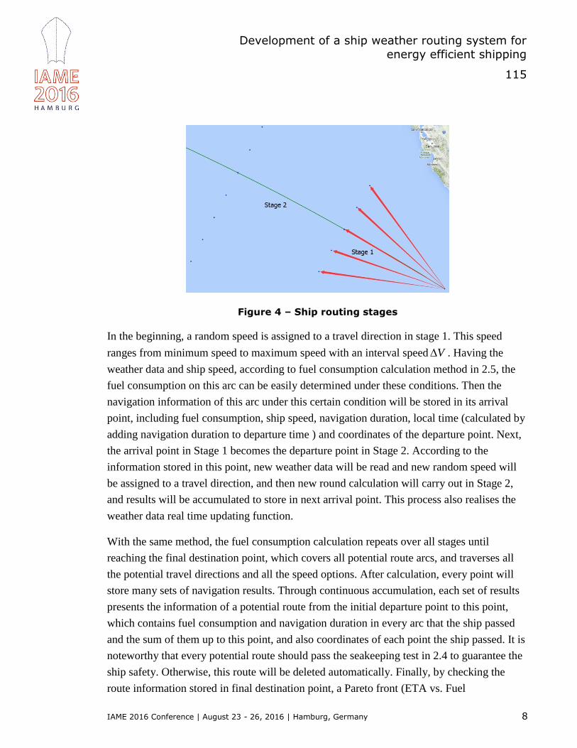
Figure 4 – Ship routing stages
In the beginning, a random speed is assigned to a travel direction in stage 1. This speed
ranges from minimum speed to maximum speed with an interval speed V . Having the
weather data and ship speed, according to fuel consumption calculation method in 2.5, the
fuel consumption on this arc can be easily determined under these conditions. Then the
navigation information of this arc under this certain condition will be stored in its arrival
point, including fuel consumption, ship speed, navigation duration, local time (calculated by
adding navigation duration to departure time ) and coordinates of the departure point. Next,
the arrival point in Stage 1 becomes the departure point in Stage 2. According to the
information stored in this point, new weather data will be read and new random speed will
be assigned to a travel direction, and then new round calculation will carry out in Stage 2,
and results will be accumulated to store in next arrival point. This process also realises the
weather data real time updating function.
With the same method, the fuel consumption calculation repeats over all stages until
reaching the final destination point, which covers all potential route arcs, and traverses all
the potential travel directions and all the speed options. After calculation, every point will
store many sets of navigation results. Through continuous accumulation, each set of results
presents the information of a potential route from the initial departure point to this point,
which contains fuel consumption and navigation duration in every arc that the ship passed
and the sum of them up to this point, and also coordinates of each point the ship passed. It is
noteworthy that every potential route should pass the seakeeping test in 2.4 to guarantee the
ship safety. Otherwise, this route will be deleted automatically. Finally, by checking the
route information stored in final destination point, a Pareto front (ETA vs. Fuel
Development of a ship weather routing system for
energy efficient shipping
115
IAME 2016 Conference | August 23 - 26, 2016 | Hamburg, Germany 9
consumption) can be drawn. Moreover, then a minimum fuel consumption and safe enough
route plan can be selected according to the ship navigation schedule (ETA). The whole
process can be regarded as a global optimisation.
By the way, when a ship travels from a stage to next, it will produce many different ETA
and fuel consumption results due to so many speed and direction options. If continuous
iteration lasts until final destination point, the quantity of final results will be prohibitively
huge. This will lead to a huge calculation cost. Here, local optimisation strategy is
introduced. For a certain arrival point, it is sure that it will receive many ETA and fuel
consumption results from the last stage. Among them, there must be some results have same
arrive time but different fuel consumption. So this method just keeps the minimum fuel
consumption under every same arrival time and deletes all of the others. Thus, keeping a
Pareto front for every local waypoint. With this method, when fuel consumption calculation
carries out from this waypoint, only the left results will be traversed. So it will definitely
save the calculation cost.
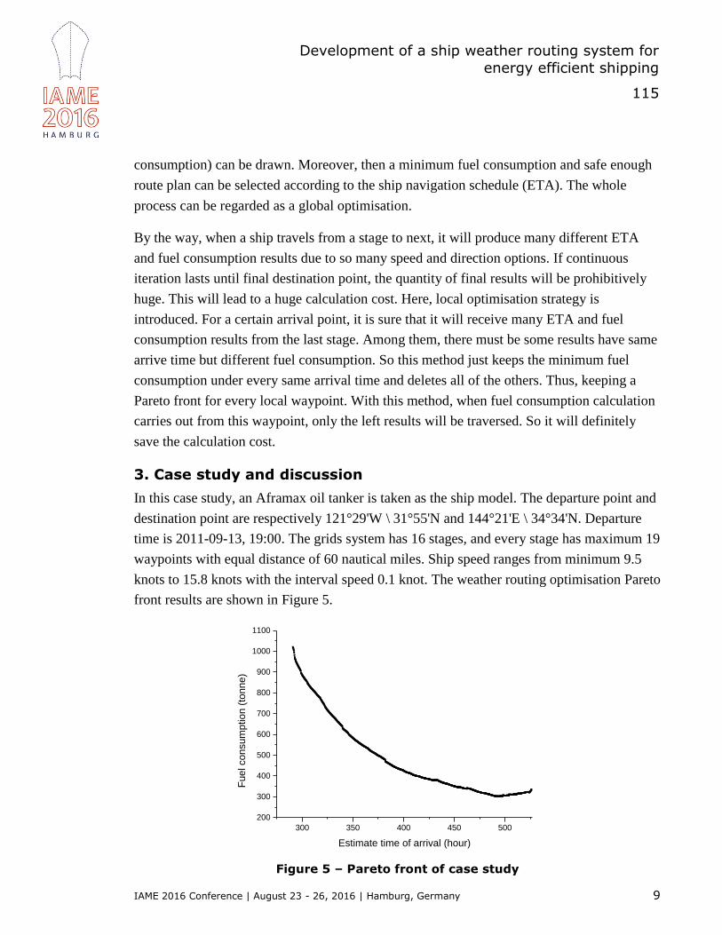
3. Case study and discussion
In this case study, an Aframax oil tanker is taken as the ship model. The departure point and
destination point are respectively 121°29'W \ 31°55'N and 144°21'E \ 34°34'N. Departure
time is 2011-09-13, 19:00. The grids system has 16 stages, and every stage has maximum 19
waypoints with equal distance of 60 nautical miles. Ship speed ranges from minimum 9.5
knots to 15.8 knots with the interval speed 0.1 knot. The weather routing optimisation Pareto
front results are shown in Figure 5.
300 350 400 450 500
200
300
400
500
600
700
800
900
1000
1100
Fuel consum
ption (
tonne)
Estimate time of arrival (hour)
Figure 5 – Pareto front of case study
Development of a ship weather routing system for
energy efficient shipping
115
IAME 2016 Conference | August 23 - 26, 2016 | Hamburg, Germany 10
It can be seen from Fig 5. There are almost 2000 potential route plans during this voyage.
The ETA ranges from 290.6 h to 528.3 h, while the fuel consumption ranges from 301.09
tonnes to 1021.19 tonnes. Speed sets, ETA and fuel consumption of four typical routes:
Noon report recorded route, 392h ETA route, Minimum fuel consumption route and
Minimum ETA route were listed in Table 1.
Table 1 – Total results
Stage
Noon report
recorded
route
392h ETA
route
Minimum
fuel
consumptio
n route
Minimum
ETA route
Speed sets
(knots)
1 12.5 12.6 9.5 15.8
2 12.6 12.8 9.5 15.8
3 12.9 12.5 9.5 15.8
4 12.6 13.2 9.5 15.8
5 12.3 12.7 9.5 15.8
6 11.9 12.8 9.5 15.8
7 11.1 9.9 9.5 15.8
8 11.7 9.6 9.5 15.8
9 11.9 9.5 9.5 15.8
10 12.8 10.9 9.5 15.8
11 12.1 10.5 9.5 15.8
12 12.8 12 9.7 15.8
13 12.3 11.9 9.7 15.8
14 10.4 12.7 9.5 15.8
15 10.5 13.4 9.5 15.8
16 9.9 14.4 9.5 15.8
ETA (hours) 392.0 392.0 492.1 290.6
Fuel consumption (tonnes) 623.3 450.98 301.09 1021.19
According to history noon report, the recorded route has 392 h of ETA and 623.3 tonnes of
fuel consumption. For the sake of comparison, the potential route with same ETA is
selected. Although their average speed is quite similar: 11.89 knots and 11.96 knots, their
speed sets have different changing trends: the recorded results are steady, while the
calculated results show the ship decelerated at the first half stages and then accelerated at the
second stages. The speed sets of the calculated route also reflect weather conditions are
changing. In that calculated route, the wind and wave condition in middle stages are worse,
so the ship should reduce the speed to guarantee the safety. When the weather becomes
Development of a ship weather routing system for
energy efficient shipping
115
IAME 2016 Conference | August 23 - 26, 2016 | Hamburg, Germany 11
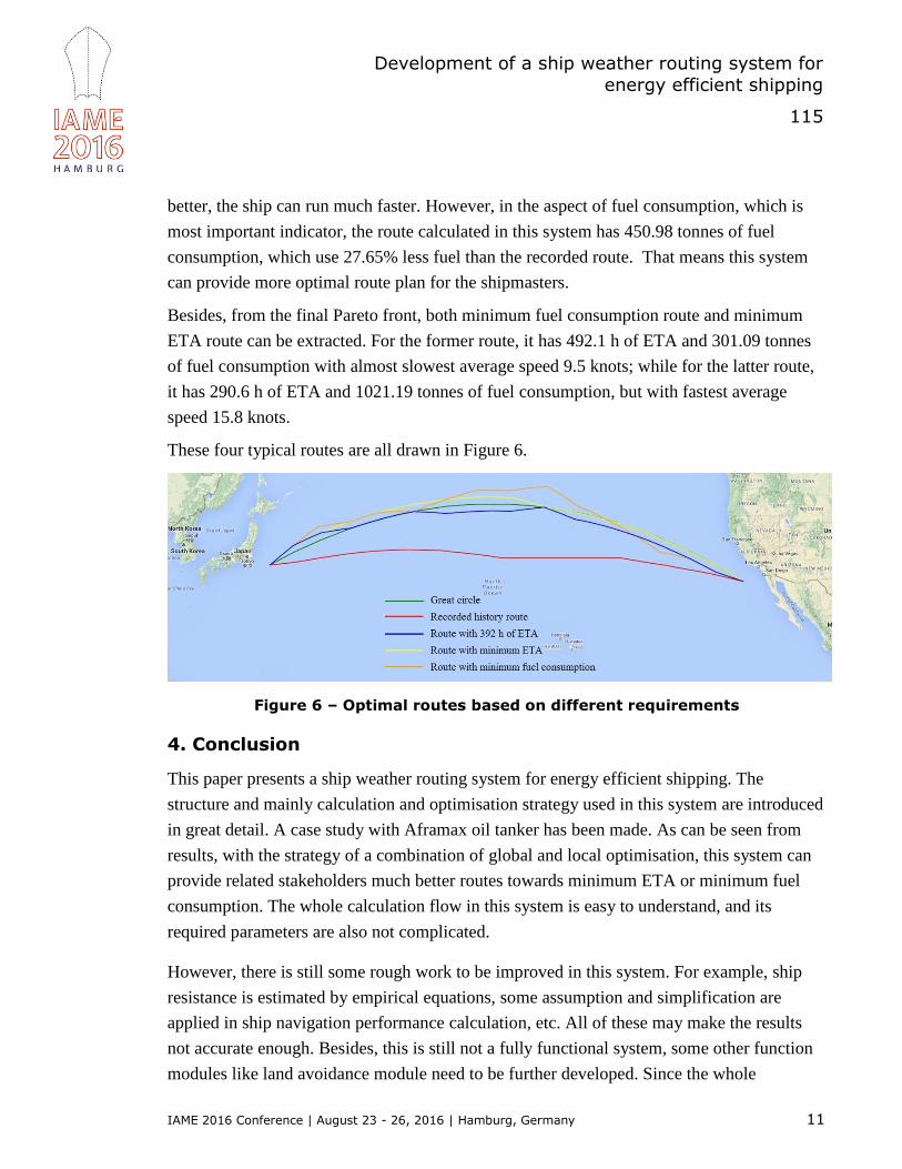
better, the ship can run much faster. However, in the aspect of fuel consumption, which is
most important indicator, the route calculated in this system has 450.98 tonnes of fuel
consumption, which use 27.65% less fuel than the recorded route. That means this system
can provide more optimal route plan for the shipmasters.
Besides, from the final Pareto front, both minimum fuel consumption route and minimum
ETA route can be extracted. For the former route, it has 492.1 h of ETA and 301.09 tonnes
of fuel consumption with almost slowest average speed 9.5 knots; while for the latter route,
it has 290.6 h of ETA and 1021.19 tonnes of fuel consumption, but with fastest average
speed 15.8 knots.
These four typical routes are all drawn in Figure 6.
Figure 6 – Optimal routes based on different requirements
4. Conclusion
This paper presents a ship weather routing system for energy efficient shipping. The
structure and mainly calculation and optimisation strategy used in this system are introduced
in great detail. A case study with Aframax oil tanker has been made. As can be seen from
results, with the strategy of a combination of global and local optimisation, this system can
provide related stakeholders much better routes towards minimum ETA or minimum fuel
consumption. The whole calculation flow in this system is easy to understand, and its
required parameters are also not complicated.
However, there is still some rough work to be improved in this system. For example, ship
resistance is estimated by empirical equations, some assumption and simplification are
applied in ship navigation performance calculation, etc. All of these may make the results
not accurate enough. Besides, this is still not a fully functional system, some other function
modules like land avoidance module need to be further developed. Since the whole

Development of a ship weather routing system for
energy efficient shipping
115
IAME 2016 Conference | August 23 - 26, 2016 | Hamburg, Germany 12
framework of this system works well, there is a reason to believe that the next generation of
the ship weather routing system in the future will become more perfect.
Acknowledgements
This research is co-sponsored by UK Research Council, University of Strathclyde and China
Scholarship Council. The authors would like to express sincere thanks for their support.
Reference
BELLMAN, R.E., 1957, Dynamic Programming. (Princeton: Princeton University Press).
BIJLSMA, S.J., 1975, On Minimal-Time Ship Routing. PhD Thesis. Royal Netherlands
Meteorological Institute, Delft University of Technology.
CALVERT, S., DEAKINS, E. and MOTTE, R., 1991, A Dynamic System for Fuel
Optimisation Trans-Ocean. Journal of Navigation, 44 (2), 233-265.
DE WIT, C., 1990, Proposal for Low Cost Ocean Weather Routeing. Journal of Navigation,
43 (3), 428-439.
ESKILD, H., 2014, Development of a method for weather routing of ships. Master Thesis.
Department of Marine Technology, Norwegian University of Science and Technology.
FALTINSEN, O. M., MINSAAS, K. J., LIAPIS, N and SKJØRDAL, S. O., 1981, Prediction
of resistance and propulsion of a ship in a seaway. 13th Symposium on Naval
Hydrodynamics Shipbuilding Research Association of Japan.
GERRITSMA, J., and BEUKELMAN, W., 1972, Analysis of the resistance increase in
waves of a fast cargo ship. International Shipbuilding Progress, 19(217), 285–293.
HAGIWARA, H. and SPAANS, J.A., 1987, Practical Weather Routeing of Sail- Assisted
Motor Vessels. Journal of Navigation, 40, 96-119.
HAGIWARA, H., 1989, Weather Routing Of (Sail-Assisted) Motor Vessels. PhD Thesis.
Delft University of Technology.
HARRIES, S., HEINMANN, J. and HINNENTHAL, J., 2003, Pareto-Optimal Routing Of
Ships. International Conference on Ship and Shipping Research, Palermo.
HINNENTHAL, J., 2010, Robust Pareto-Optimum Routing of Ships Utilising Deterministic
and Ensemble Weather Forecasts. PhD Thesis. Technische Universität Berlin.

Development of a ship weather routing system for
energy efficient shipping
115
IAME 2016 Conference | August 23 - 26, 2016 | Hamburg, Germany 13
HOLTROP, J., 1984, A Statistical Re-Analysis of Resistance and Propulsion Data.
International Shipbuilding Progress, 31(363), 272-276.
JAMES, R.W., 1957, Application of wave forecasts to marine navigation. Washington DC:
Navy Hydrographic Office.
KLOMPSTRA, M.B. et al., 1992, The Isopone Method in Optimal Control. Dynamics and
Control, 2(3), 281-301.
LO, H. and McCORD, M., 1998, Adaptive ship routing through stochastic ocean currents
general formulations and empirical results, Transportation Research Part A: Policy and
Practice, 32(7), 547–561
LOUKAKIS, T.A., and SCLAVOUNOS, P.D., 1978. Some extensions of the classical
approach to strip theory of ship motions, including the calculation of mean added forces and
moments. Journal of Ship Research, 22(1), 1–19.
McCORD, M. LEE Y. and LO, H., 1999, Ship routing through altimetry-derived ocean
currents, Transportation Science, 33(1), 49-67
MINSAAS, K., FALTINSEN, O. M. and PERSSON, B., 1983, On the importance of added
resistance, propeller immersion and propeller ventilation for large ships in a seaway. 2nd
International Symposium on Practical Design in Shipbuilding (PRADS`83), Tokyo & Seoul,
October, 149-159.
NORDFORSK, 1987. Assessment of a ship performance in a seaway.
PADHY, C.P, SEN, D. and BHASKARAN, P.K. 2008, Application of wave model for
weather routing of ships in the North Indian Ocean’. Natural Hazards, 44(3), 373–385.
PANIGRAHI, J.K. and UMESH, P.A., 2008, Minimal Time Ship Routing Using IRSP4
(MSMR) Analyzed Wind Fields. Marine Geodesy, 31(1), 39–48.
SHAO, W., ZHOU, P., THONG, S. K., 2012, Development of a novel forward dynamic
programming method for weather routing. Journal of Marine Science and Technology
17(2), 239–251.
SPAANS, J.A., 1995, New Developments in Ship Weather Routing. Navigation, 169, 95-
106.

Development of a ship weather routing system for
energy efficient shipping
115
IAME 2016 Conference | August 23 - 26, 2016 | Hamburg, Germany 14
SZLAPCZY´NSKA, J. and SMIERZCHALSKI, R., 2007, Adopted Isochrones Method
Improving Ship Safety in Weather Routing With Evolutionary Approach. International
Journal of Reliability, Quality and Safety Engineering, 14(6), 635-645.


![Weather Routing [J-Marine Routing] The global maritime ... · This service provides the weather routing information to support the safety and economy of ship navigation and realizes](https://cdn.vdocuments.us/doc/165x107/5afca6e37f8b9a814d8c6581/weather-routing-j-marine-routing-the-global-maritime-service-provides-the.jpg)


