
ME5542
Advanced Modelling and Design
AME Mechanical Engineering
School of Engineering and Design
Brunel University
Uxbridge
UK
Advanced Modelling and Design, Mechanical Engineering, March 2011 1 of 16 W.R. Shipway
Design Optimisation – Use of golden section
search method in the design of a new
removable orthopedic device
Conference on the Implementation of New Advances in Engineering Design 2011
W.R. Shipway
Abstract
The Golden Section Search Method is described, and employed for a number of variables in the
design of a new removable orthopedic device. The pertaining variables involved in the method
are elucidated, including the boundaries and tolerance, and derivation of the golden ratio. The
boundaries and tolerance are discussed in detail and advice is formed and presented on the
optimum selection of these variables. The qualities and limitations of the method are discussed,
and the uncertainties in applying the method are deliberated. The efficiency is compared with a
similar optimisation method (Fibonacci Method– not explained), and it is suggested when to
use each method. The results of the design variables in the example application show
convergence on the extremum of non-linear functions. Evidence is provided for the (already
known) extremum‟s to show comparisons between the method and an exact solution obtained
analytically. Engineering applications of the method are summarized, and more general
applications are suggested, including economics and manufacturing, relating the use of the
method to within an organisation. Excel is employed in the design application, but the use of a
Matlab command is suggested as another way of utilizing GSS.
Keywords: Golden Section Search Method, design factors, unimodal optimisation, orthopedic
device
1. Introduction
The (GSS) method is an iterative procedure for reducing the region where a solution to a
unimodal function may lie. All iteration methods describe a procedure by which the root(s) of
an equation (set of equations) can be found by repeatedly (iteratively) reducing the boundaries
that the minimum (or maximum, named here as extremum) may lie. [Yakowitz, 1974, p. 234]
The pertaining alterable quantities that define this procedure are the boundaries which the roots
lie within, and the reduction method, irrespective of the equation itself. The two defining
quantities are intrinsically related, with the boundary being thus reduced at each iteration. The
procedure is to define the boundaries, inspect the solution at a (undefined thus far) point at a
distance from the boundary, and adjust the boundaries so that the new point becomes a
boundary itself. The new inspection point would be in-between the new boundary and the
remaining original boundary. Which boundary is replaced is dependent on whether the solution
is closer to the desired solution or not (i.e. the extremum).

2 of 16
Logically, the most obvious reduction method is to half the area in which the solution may lie
with each iteration, and is known as the bisection method [Press, 1992, p. 353]. It is considered
obvious as any method using a reduction of more than half may yield the solution in the other
region (i.e. 1 – (>0.5)) and thus be less than half. However, the GSS is known to be a more
efficient method of finding a solution iteratively, and was first deliberated in 1953 by Kiefer
[Kiefer, 1953, pp. 502-506]. Kiefer makes no mention of the golden ratio itself, but derives the
interval length similar to as shown in this paper.
The golden ratio is intuitively intriguing due to its abundance in natural phenomena. It is
defined in the context of this paper as (traced back to Phidias [Hemenway, 2005]);
Length of inspecting region
Length of larger interval=
Length of larger interval
Length of smaller interval
If the length of inspecting region is of unity and φ (phi – after Phidias) denotes the length of the
larger interval (so that the smaller interval is 1 – φ) then expressing mathematically,
1
φ=
φ
1 − φ (1)
The general form resolves to,
1
φ=
φ
1 − φ⟹ φ2 = 1 − φ ⟹ φ2 + φ − 1 = 0
With the solution to the quadratic equation found as,
ax2 + bx + c = 0 ⟹ x1, x2 =−b ± b2 − 4ac
2 × 1;
φ =−1 ± 12 − [4 × 1 × −1 ]
2 × 1=−1 ± 1 + 4
2
With the positive solution as the irrational number,
φ =−1 + 5
2= 0.61833988749895… (2)
- Procedure
Consider a function f(x) which follows the form shown in Fig. 1. The points x1 and x2 are at
lengths of the golden ratio from the boundaries (limits) B1 and B2.

3 of 16
Figure 1. An arbitrary unimodal solution f(x), with upper and lower limits.
The lengths of the arrows can be calculated via different methods, all relating to φ. They are
shown in Fig. 2.
Figure 2. Various ways to calculate the inspection points x1 and x2 with the limits B1 and B2.
Once the initial inspection points have been determined from use of the equations stated in Fig.
2 they can be evaluated and the interval reduced. One of the inspection points will be less than
the second. The larger function root will then be replaced as the new limit. If, as is shown in
Fig. 2, x2 is smaller than x1 then x1 becomes B1 and a new inspection point will be created. This
point will be at a distance of the golden ratio from the new boundary. If x2 were larger than x1
then x2 would become the new boundary and a new inspection point would form at a distance
from x2.
Reiterating mathematically, if x2 < x1 then B1 = x1 with the new boundaries at B2 and x1, and the
new inspection point is x3 = (B2 – x1)(1 – φ). The two inspection points for the second iteration
are now (the same) x2 and (the new) x3, and will again be compared, with the appropriate

4 of 16
(larger) inspection point being replaced to form the new boundary. Note in Fig. 2 the
symmetrical nature of the distances, so that the distance from B1 = (B2 – B1)(1 – φ) is the same
as the distance x1 from B1 (hence the use of the expression in the above iteration). The new
inspection points will then look as is shown in Fig. 3.
Figure 3. After one iteration the points of inspection will be (the same) x2 and (the new) x3.
Clearly, the reduction has „jumped‟ over the solution of minimising f(x), but as it still lies
within the boundaries the proceeding iterations will converge upon that point.
- Termination condition
At some point the iterations must be concluded, upon which the final value is found and the
decision is taken for that to be the solution. This must be decided upon before the method is
introduced to the problem, and can be as simple as a limit on the number of iterations.
- Applications
The main application of the GSS method may be used when the governing equations are not
differentiable, or when the solution is not easily obtainable, when differentiation proves too
complex practically. Examples include natural phenomenon: activation energy of a chemical
reaction [Cai, 2010], approximate language reasoning interpretations (fuzzy linguistics – a
pressing matter in quality of information) [Leephakpreeda, 2006]; partial differential equations
(PDE‟s): determining the shape of a statistical distribution in the use of mesh free methods for
numerical simulations of PDE‟s [Tsai, 2010]; and more generally in engineering it is applied to
solutions in complex fluid mechanics modelling (non-newtonian fluids [Ohen, 1990] and
thermal conductivity with unknown coefficients [Mierzwiczak, 2011]). But, it can be applied to
all extremum and optimisation methods of a unimodal form with no derivatives.
- A Note on the Golden Ratio The actual golden ratio is φR = 1.618… where φ = 1/φR and is the ratio of the larger to smaller
interval, not the length of the larger interval, and some sources derive the value at 1.618. But
when applied all cited sources should and will use 0.618 in application. This is because to have
a new inspection point at 1.618 times the interval would not reduce the inspection region at all!
5 of 16
2. Method
As described in the previous section, applications of the GSS method are typically difficult to
solve with classical methods, and therefore the GSS is not utilized for common engineering
problems easily. Here the application of the method is straightforward for two reasons – 1. So
the application is understood to the reader, and 2. Verification is possible. If the application is
complex and “real world” then absolute verification would be complex, time consuming and/or
costly. Also, this application will highlight limitations in the method that may otherwise not be
apparent.
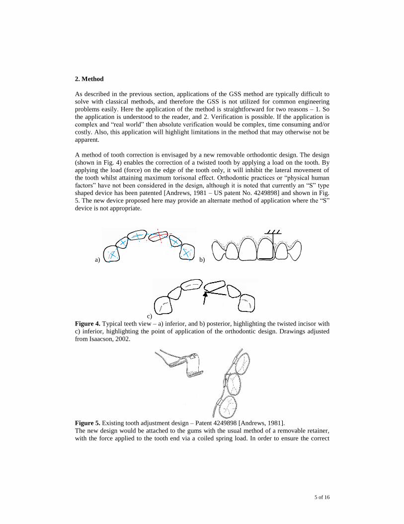
A method of tooth correction is envisaged by a new removable orthodontic design. The design
(shown in Fig. 4) enables the correction of a twisted tooth by applying a load on the tooth. By
applying the load (force) on the edge of the tooth only, it will inhibit the lateral movement of
the tooth whilst attaining maximum torisonal effect. Orthodontic practices or “physical human
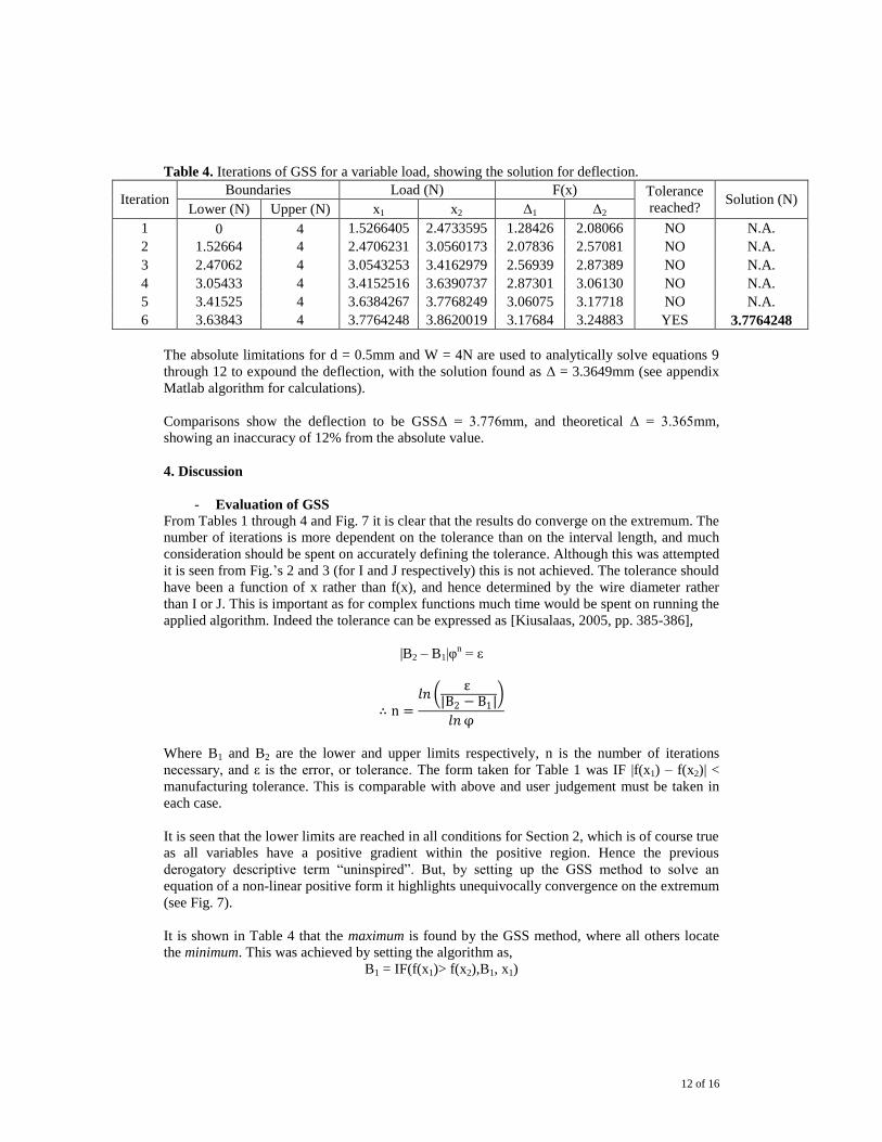
factors” have not been considered in the design, although it is noted that currently an “S” type
shaped device has been patented [Andrews, 1981 – US patent No. 4249898] and shown in Fig.
5. The new device proposed here may provide an alternate method of application where the “S”
device is not appropriate.
a) b)
c)
Figure 4. Typical teeth view – a) inferior, and b) posterior, highlighting the twisted incisor with
c) inferior, highlighting the point of application of the orthodontic design. Drawings adjusted
from Isaacson, 2002.
Figure 5. Existing tooth adjustment design – Patent 4249898 [Andrews, 1981].
The new design would be attached to the gums with the usual method of a removable retainer,
with the force applied to the tooth end via a coiled spring load. In order to ensure the correct

6 of 16
load is achieved the deflection of the device is approximated if it were free. At this point the
load on the tooth is removed as the device has reached full extension, and the tooth has been
corrected. It is seen from Fig. 4b that the device can be modelled as a cranked cantilever with
the applied force in the perpendicular direction.
The use of the GSS method is applied to the cranked cantilever. An example design is shown in
Fig. 6. The free end is subjected to a load, W, and will deflect by Δ. This is dependent on a
number of factors. The contributing variables are:
Geometrically – cross sectional area (A)
second moment of area (I)
polar moment of inertia (J)
lengths of the bar sections (L1 and L2)
Materially – modulus of elasticity (E)
modulus of rigidity (G)
Figure 6. The cranked cantilever model of the orthopedic design.
The general governing equations that define the deflection according to strain energy methods
are (Rees, 1997),
Shear energy, U =1
2G
W2x
A
L
0
. dx (3)
Bending moment energy, U =1
2E
M2x
I
L
0
. dx (4)
Torsional moment energy, U =1
2G
T2x
J
L
0
. dx (5)
Where M is the moment and T is the applied torque at the end of the bar section.

7 of 16
The displacement is governed by Castigliano‟s second theorem,
Δ =∂U
∂W (6)
From Fig. 6 it is seen that the length L1 is subjected to shear and bending, and L2 is subjected to
shear, bending and torsion (where T = WL1). The explicit forms are thus,
UL1 =1
2G
W2x
A
L
0
. dx + 1
2E
M2x
I
L
0
. dx
=W2L1
2AG+
W2L13
6EI
= L1
2AG+
L13
6EI W2 (7)
UL2 =1
2G
W2x
A
L
0
. dx + 1
2E
M2x
I
L
0
. dx +1
2G
T2x
J
L
0
. dx
=W2L2
2AG+
W2L23
6EI+ WL1
2L2
2GJ
= L2
2AG+
L23
6EI+
L12L2
2GJ W2 (8)
Where,
A =πd2
4= πr2 (9)
I =πd4
64=πr4
4 (10)
J =πd4
32=πr4
2 (11)
The deflection is thus,
U =WΔ
2 ⟹ Δ =
2 U
W
Δ = 2 × L1
2AG+
L13
6EI+
L2
2AG+
L23
6EI+
L12L2
2GJ W 12

8 of 16
It is seen from equations 9 to 11 that the devices material and geometrical variables are only a
function of the diameter of the wire, but the form (graphical representation) will be different for
each function.
Considerations on the boundary conditions (constraints) include:
- The wire diameter should not be less than 0.5mm. As stated in Removable Orthodontic
Appliances - “the patient would readily distort thinner (than 0.5mm) wire and they are
not generally recommended” [Isaacson, 2002, p.18]
- The upper boundary of the wire diameter is 1.5mm. A larger size than this would
produce discomfort to the user.
- The lengths L1 and L2 are defined by a population evaluation of incisor size, and found
to be 8.47mm (SD 1.2) and width 6.84mm (SD 0.9) [Seper, 2006, pp. 59-60]. This
does not include children, as the use of an orthopedic device on deciduous teeth would
be fruitless. Also the variation does not include microdontia or macrodontia
(abnormally small/large teeth respectively). The limits are then for L1 = 5.94mm to
7.74mm, L2 = 7.27mm to 9.67mm.
The wire diameter minimum is defined due to the limits of elasticity. However, 0.5mm is not
necessarily the minimum as it is intrinsic to the material properties. Hence the boundaries
defined are a product of the elastic limit, which is in turn limited by the cost, manufacturability,
and legality regarding materials in-vivo the human body. Due to said legality reasons there is
only one spring material considered, that of stainless steel, with (approximate) properties of E =
203 GPa and G = 80 GPa. The wire diameter then determines the limits of A, I, and J as:
A = 0.196mm2 to 1.767mm
2
I = 0.00307mm4 to 0.249mm
4
J = 0.00614mm4 to 0.497mm
4
The deflection must also be considered. The maximum deflection necessary for the device
would be if the incisor were twisted by 90o. Beyond this point the location of the device would
be moved to the other side. Thus the maximum deflection would be a small amount less than
half the width of the incisor, because if the incisor were at 90o the device would no longer be
attributed to a twisting effect – it would be a lateral adjustment. However, the deflection is
considered a function of the lengths, as a smaller/larger length L1 and L2 will adjust the
deflection defined in equations 7 and 8.
The tolerance must now be defined, so that the iterations will be terminated whence the desired
accuracy is reached. Considering again manufacturability issues the wire diameter will only be
capable of certain finite changes in size. The lengths L1 and L2 are simultaneously products of
equation 12. Thus once the iterations reduce the variables by less than the defined tolerance any
further iterations would be ineffective as they will not be practical.
Tol. –
d = 0.05mm
Hence tol. –
A = 0.00196mm2
I = 3.068×10⁻⁷
mm4
J = 6.136×10⁻⁷
mm4

9 of 16
The GSS method is then employed to use these limits and tolerances to define the minimum of
A, I, and J according to equations 7 through 11 by use of a table, with L1 = 7.74mm and L2 =
9.67mm. The deflection is then maximised by use of equations 7, 8 and 12, with the limits of
force defined as a function of the number of coils in the spring, from 0N to 4N.
3. Results
The results shown in Table 1 through 5 are that of the GSS method. The lengths are evaluated
from equation 12 once the minimum of A, I and J are defined. The results are compared with
that obtained analytically by use of equations 7 through 12.
Note: the extra columns are for procedural clarification, and in practice an algorithm would be
employed. The extra iterations are to show convergence is achieved, as is shown in Fig. 7.
Table 1. Iterations of GSS for the diameter as a function of the area.
Iteration
Boundaries Wire Diameter (mm) F(x) (mm2)
Tolerance
reached? Solution(mm
2)
Lower
(mm)
Upper
(mm) x1 x2 A1 A2
1 0.5 1.50000 0.88166 1.11834 0.61051 0.98228 NO N.A. 3
2 0.5 1.11834 0.73600 0.88234 0.42544 0.61146 NO N.A. 4
3 0.5 0.88234 0.64593 0.73642 0.32768 0.42593 NO N.A. 5
4 0.5 0.73642 0.59023 0.64619 0.27361 0.32795 NO N.A. 6
5 0.5 0.64619 0.55579 0.59039 0.24261 0.27376 NO N.A. 7
6 0.5 0.59039 0.53450 0.55589 0.22438 0.24270 NO N.A. 8
7 0.5 0.55589 0.52133 0.53456 0.21346 0.22443 NO N.A. 9
8 0.5 0.53456 0.51319 0.52137 0.20685 0.21349 NO N.A. 10
9 0.5 0.52137 0.50816 0.51321 0.20281 0.20687 NO N.A. 11
10 0.5 0.51321 0.50504 0.50817 0.20033 0.20282 NO N.A. 12
11 0.5 0.50817 0.50312 0.50505 0.19881 0.20034 YES 0.50312 13
12 0.5 0.50505 0.50193 0.50312 0.19787 0.19881 YES 0.50193 14
13 0.5 0.50312 0.50119 0.50193 0.19729 0.19787 YES 0.50119 15
14 0.5 0.50193 0.50074 0.50119 0.19693 0.19729 YES 0.50074 16
15 0.5 0.50119 0.50046 0.50074 0.19671 0.19693 YES 0.50046 17
16 0.5 0.50074 0.50028 0.50046 0.19657 0.19671 YES 0.50028 18
17 0.5 0.50046 0.50017 0.50028 0.19649 0.19657 YES 0.50017 19
18 0.5 0.50028 0.50011 0.50017 0.19643 0.19649 YES 0.50011 20
A B C D E F G H I
The formula employed in Excel is:
Lower Boundary = IF(F3<G3,B3,D3)
Upper Boundary = IF(F3<G3,E3,C3)
x1 = C4-(0.618339887498*(C4-B4)) % from Fig. 2
x2 = B4+(0.618339887498*(C4-B4)) % from Fig. 2
A1 = PI()*(D4/2)^2
A2 = PI()*(E4/2)^2

10 of 16
Tolerance Reached? = IF((ABS(G4-F4)<0.00196),"YES","NO")
Solution = IF(H4="YES",IF(F4<G4,F4,G4),"N.A.")
Figure 7. A convergence check, ensuring that the diameter is converging upon the minimum
Table 2. Iterations of GSS for the diameter as a function of the second moment of area.
Iteration
Boundaries Wire Diameter (mm) F(x) (mm4)
Tolerance
reached?
Solution
(mm4)
Lower
(mm)
Upper
(mm) x1 x2 I1 I2
1 0.5 1.5 0.8816601 1.1183399 0.0296602 0.0767830 NO N.A.
2 0.5 1.1183399 0.7359957 0.8823442 0.0144036 0.0297524 NO N.A.
3 0.5 0.8823442 0.6459255 0.7364187 0.0085448 0.0144367 NO N.A.
4 0.5 0.7364187 0.5902316 0.6461871 0.0059574 0.0085586 NO N.A.
5 0.5 0.6461871 0.5557938 0.5903933 0.0046841 0.0059640 NO N.A.
6 0.5 0.5903933 0.5344995 0.5558938 0.0040064 0.0046875 NO N.A.
7 0.5 0.5558938 0.5213324 0.5345614 0.0036260 0.0040083 NO N.A.
8 0.5 0.5345614 0.5131907 0.5213707 0.0034047 0.0036271 NO N.A.
9 0.5 0.5213707 0.5081563 0.5132143 0.0032731 0.0034054 NO N.A.
10 0.5 0.5132143 0.5050434 0.5081710 0.0031936 0.0032735 NO N.A.
11 0.5 0.5081710 0.5031185 0.5050524 0.0031452 0.0031939 NO N.A.
12 0.5 0.5050524 0.5019283 0.5031241 0.0031156 0.0031454 NO N.A.
13 0.5 0.5031241 0.5011924 0.5019318 0.0030973 0.0031156 NO N.A.
14 0.5 0.5019318 0.5007373 0.5011945 0.0030861 0.0030974 NO N.A.
15 0.5 0.5011945 0.5004559 0.5007386 0.0030792 0.0030861 NO N.A.
16 0.5 0.5007386 0.5002819 0.5004567 0.0030749 0.0030792 NO N.A.
0.0
0.2
0.4
0.6
0.8
1.0
1.2
0 2 4 6 8 10
Wir
e C
ross
sec
tio
nal
are
a (m
m2)
Iteration No.
Convergence on Minimum Wire X-secion Area
A1 A2

11 of 16
Table 2. Continued
17 0.5 0.5004567 0.5001743 0.5002824 0.0030722 0.0030749 NO N.A.
18 0.5 0.5002824 0.5001078 0.5001746 0.0030706 0.0030722 NO N.A.
19 0.5 0.5001746 0.5000666 0.5001080 0.0030696 0.0030706 NO N.A.
20 0.5 0.5001080 0.5000412 0.5000668 0.0030690 0.0030696 NO N.A.
21 0.5 0.5000668 0.5000255 0.5000413 0.0030686 0.0030690 NO N.A.
22 0.5 0.5000413 0.5000158 0.5000255 0.0030683 0.0030686 YES 0.5000158
Table 3. Iterations of GSS for the diameter as a function of the polar moment of inertia.
Iteration
Boundaries Wire Diameter (mm) F(x) (mm4)
Tolerance
reached?
Solution
(mm4)
Lower
(mm)
Upper
(mm) x1 x2 J1 J2
1 0.5 1.5000000 0.8816601 1.1183399 0.0593205 0.1535660 NO N.A.
2 0.5 1.1183399 0.7359957 0.8823442 0.0288072 0.0595048 NO N.A.
3 0.5 0.8823442 0.6459255 0.7364187 0.0170895 0.0288735 NO N.A.
4 0.5 0.7364187 0.5902316 0.6461871 0.0119149 0.0171172 NO N.A.
5 0.5 0.6461871 0.5557938 0.5903933 0.0093682 0.0119279 NO N.A.
6 0.5 0.5903933 0.5344995 0.5558938 0.0080129 0.0093749 NO N.A.
7 0.5 0.5558938 0.5213324 0.5345614 0.0072520 0.0080166 NO N.A.
8 0.5 0.5345614 0.5131907 0.5213707 0.0068095 0.0072541 NO N.A.
9 0.5 0.5213707 0.5081563 0.5132143 0.0065462 0.0068108 NO N.A.
10 0.5 0.5132143 0.5050434 0.5081710 0.0063873 0.0065470 NO N.A.
11 0.5 0.5081710 0.5031185 0.5050524 0.0062904 0.0063877 NO N.A.
12 0.5 0.5050524 0.5019283 0.5031241 0.0062311 0.0062907 NO N.A.
13 0.5 0.5031241 0.5011924 0.5019318 0.0061947 0.0062313 NO N.A.
14 0.5 0.5019318 0.5007373 0.5011945 0.0061722 0.0061948 NO N.A.
15 0.5 0.5011945 0.5004559 0.5007386 0.0061583 0.0061723 NO N.A.
16 0.5 0.5007386 0.5002819 0.5004567 0.0061498 0.0061584 NO N.A.
17 0.5 0.5004567 0.5001743 0.5002824 0.0061445 0.0061498 NO N.A.
18 0.5 0.5002824 0.5001078 0.5001746 0.0061412 0.0061445 NO N.A.
19 0.5 0.5001746 0.5000666 0.5001080 0.0061392 0.0061412 NO N.A.
20 0.5 0.5001080 0.5000412 0.5000668 0.0061379 0.0061392 NO N.A.
21 0.5 0.5000668 0.5000255 0.5000413 0.0061372 0.0061379 NO N.A.
22 0.5 0.5000413 0.5000158 0.5000255 0.0061367 0.0061372 YES 0.5000158
The diameter is thus the smallest of the values obtained in Tables 1 through 3. As I = J < A, so
d = 0.5000158. Note this is only due to the tolerance inaccuracies, with a solution of the area
found in 11 iterations.
12 of 16
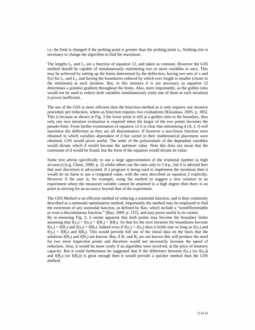
Table 4. Iterations of GSS for a variable load, showing the solution for deflection.
Iteration Boundaries Load (N) F(x) Tolerance
reached? Solution (N)
Lower (N) Upper (N) x1 x2 Δ1 Δ2
1 0 4 1.5266405 2.4733595 1.28426 2.08066 NO N.A.
2 1.52664 4 2.4706231 3.0560173 2.07836 2.57081 NO N.A.
3 2.47062 4 3.0543253 3.4162979 2.56939 2.87389 NO N.A.
4 3.05433 4 3.4152516 3.6390737 2.87301 3.06130 NO N.A.
5 3.41525 4 3.6384267 3.7768249 3.06075 3.17718 NO N.A.
6 3.63843 4 3.7764248 3.8620019 3.17684 3.24883 YES 3.7764248
The absolute limitations for d = 0.5mm and W = 4N are used to analytically solve equations 9
through 12 to expound the deflection, with the solution found as Δ = 3.3649mm (see appendix
Matlab algorithm for calculations).
Comparisons show the deflection to be GSSΔ = 3.776mm, and theoretical Δ = 3.365mm,
showing an inaccuracy of 12% from the absolute value.
4. Discussion
- Evaluation of GSS
From Tables 1 through 4 and Fig. 7 it is clear that the results do converge on the extremum. The
number of iterations is more dependent on the tolerance than on the interval length, and much
consideration should be spent on accurately defining the tolerance. Although this was attempted
it is seen from Fig.‟s 2 and 3 (for I and J respectively) this is not achieved. The tolerance should
have been a function of x rather than f(x), and hence determined by the wire diameter rather
than I or J. This is important as for complex functions much time would be spent on running the
applied algorithm. Indeed the tolerance can be expressed as [Kiusalaas, 2005, pp. 385-386],
|B2 – B1|φn = ε
∴ n =𝑙𝑛
ε |B2 − B1|
𝑙𝑛φ
Where B1 and B2 are the lower and upper limits respectively, n is the number of iterations
necessary, and ε is the error, or tolerance. The form taken for Table 1 was IF |f(x1) – f(x2)| <
manufacturing tolerance. This is comparable with above and user judgement must be taken in
each case.
It is seen that the lower limits are reached in all conditions for Section 2, which is of course true
as all variables have a positive gradient within the positive region. Hence the previous
derogatory descriptive term “uninspired”. But, by setting up the GSS method to solve an
equation of a non-linear positive form it highlights unequivocally convergence on the extremum
(see Fig. 7).
It is shown in Table 4 that the maximum is found by the GSS method, where all others locate
the minimum. This was achieved by setting the algorithm as,
B1 = IF(f(x1)> f(x2),B1, x1)
13 of 16
i.e. the limit is changed if the probing point is greater than the probing point x2. Nothing else is
necessary to change the algorithm to find the maximum.
The lengths L1 and L2 are a function of equation 12, and taken as constant. However the GSS
method should be capable of simultaneously minimising two or more variables at once. This
may be achieved by setting up the limits determined by the deflection, having two sets of x and
f(x) for L1 and L2, and having the boundaries reduced by which ever length is smaller (closer to
the minimum) at each iteration. But, in this instance it is not necessary as equation 12
determines a positive gradient throughout the limits. Also, more importantly, as the golden ratio
would not be used to reduce both variables simultaneously (only one of them at each iteration)
it proves inefficient.
The use of the GSS is more efficient than the bisection method as it only requires one iterative
procedure per reduction, where-as bisection requires two evaluations [Kiusalaas, 2005, p. 385].
This is because as shown in Fig. 3 the lower point is still at a golden ratio to the boundary, thus
only one new iteration evaluation is required when the larger of the two points becomes the
pseudo-limit. From further examination of equation 12 it is clear that minimising d (A, I, J) will
maximize the deflection as they are all denominators. If however a non-linear function were
obtained in which variables dependant of d but varied in their mathematical placement were
obtained, GSS would prove useful. The order of the polynomials of the dependant variables
would dictate which d would become the optimum value. Note this does not mean that the
extremum of d would be found, but the form of the equation would dictate its value.
Some text advise specifically to use a large approximation of the irrational number (a high
accuracy) [e.g. Chase, 2000, p. 3] whilst others use the ratio only to 3 d.p., but it is advised here
that user discretion is advocated. If a program is being used to implement the iterations then it
would do no harm to use a computed value, with the ratio described as equation 2 explicitly.
However if the user is, for example, using the method to suggest a new solution in an
experiment where the measured variable cannot be attainted to a high degree then there is no
point in striving for an accuracy beyond that of the experiment.
The GSS Method is an efficient method of reducing a unimodal function, and is thus commonly
described as a unimodal optimisation method. Importantly the method may be employed to find
the extremum of any unimodal function, as defined by Rao, which include a “nondifferentiable
or even a discontinuous function.” [Rao, 2009, p. 253], and may prove useful in its variety.
By re-assessing Fig. 3, it seems apparent that both points may become the boundary limits
assuming that f(x1) < f(x2) < f(B1) < f(B2). So that for the next iteration the boundaries become
f(x1) = f(B1) and f(x2) = f(B2). Indeed even if f(x1) > f(x2) then it holds true so long as f(x1) and
f(x2) < f(B1) and f(B2). This would provide full use of the initial data on the basis that the
solutions f(B1) and f(B2) are known. But, if B1 and B2 are not known this will produce the need
for two more inspection points and therefore would not necessarily increase the speed of
reduction. Also, it would be more costly if an algorithm were involved, at the price of memory
capacity. But it could furthermore be suggested that if the difference between f(x1) (or f(x2))
and f(B1) (or f(B2)) is great enough then it would provide a quicker method than the GSS
method.
14 of 16
- Limitations
1. The use of “local” minimum brings some complexities to practical applications of the
method (and any other iteration extremum methods). How do you know you have
reached the minimum? Or most precisely how do you know the boundaries have
defined a local? Hence the term unimodal optimisation, that it only has one extremum.
However, in practical applications the general form of the solution (equation or
experimental variables) may not be known, thus it may not be a unimodal function,
both locally and globally.
2. The specific Matlab command (see „Implementation of GSS in a Co.‟ below) does not
inspect the solution at the boundaries, so in the example application the solution would
be limited by how close the inspection gets (known as the termination tolerance or
condition).
3. The general termination condition would suggest that the value produced by use of
GSS will never reach the theoretical extremum. This phenomenon is analogous to
many topics in physics and other sciences, for example attaining a zero absolute
temperature, or reaching the speed of light. Mathematically, the GSS unobtainable
extremum is (almost) an exact representation of an asymptote in analytical geometry.
An exception would be that if the evaluating point happens to be the minimum - by
luck.
- Implementation of GSS in a Co.
The GSS method could be applied within an engineering testing and experimentation
environment. The application of optimisation within experiments is well documented, including
the use of Taguchi Methods, for multivariable experiments. But finding the optimum solution to
an engineering problem with a single variable can apply this method to reduce the time and
assets. This is a practical application, where the solution is not defined analytically or
computationally. This was actually the original proposed application of GSS by Kiefer [Kiefer,
1953, p.505]. By having no previous experimental data the next potential root can be assessed
by this method. This may be a simple application (boundaries not withstanding), but said
applications are numerous. When the number of experiments is limited and defined, the
Fibonacci Search or other methods may be applied, but when the number of experiments are
unknown the Golden Section Search can be employed. Comparatively, GSS will produce a
length 1.17 times longer [Kiefer, 1953, p. 505] than from the use of the Fibonacci search, which
is a 17% longer interval [Beighter, C.S., 1979, p. 188]). This is one of the main advantages of
the GSS, that it requires the “least prior information” [Beighter, 1979, p.186].
The GSS method may be a particularly useful tool in the economics of a cost function. The cost
of manufacturing a product decreases as the quantity of produce increases. However, at some
point the form of the function will increase as the increase of cost out-weighs the decreasing
cost-per-item value. At this point there lies a minimum where the productivity/cost curve is at
an optimal. If this method were employed it could have massive effects on the profitability and
operation and management of the Co., but is completely dependent on the Co.‟s current
techniques used. Obviously the cost function is not employed as the example in the Method
Section as verification would prove impossible without access to a Co.‟s accounts. Another
potential use is in finding the robustness (performance criteria) of a design, in the form of a
Gaussian distribution.
The use of GSS in a company is easily employable to CAE with Matlab. There is an algorithm
“fminbnd” which employs the use of the GSS method (Mathworks, 2011). The algorithm is

15 of 16
already written, with the single command above invoked to produce a result. Setup involves
creating a function handle of the function f(x), and entering the command fminbnd<name of
f(x)>(B1,B2) where, as before, Bn are the limits of the function. The tolerance is handled as
TolX. To see the description of the algorithm employed type doc fminbnd into Matlab.
5. Conclusions
The GSS method provides an iterative extremum solution. If a design problem is of a unimodal
form which is difficult or impossible to differentiate, or is discontinuous, and can be expressed
as a function then the implementation of said function with the Golden Section Search method
is of value. The method may be employed more usefully in an economic or productivity and
profitability environment. Matlab will readily invoke a rapid solution if setup is achieved. It
provides an efficient technique of locating the extremum, particularly if the number of
experiments (or iterations) is unknown. The tolerance is of great importance to efficiency of the
GSS method.
References
Andrews, L. F., 1981, Orthodontic rotation spring, La Jolla, CA, United States, PA.4249898
Beighter, C.S., Phillips, D. T., 1979, Foundations of Optimisation, 2nd
Ed., Prentice-Hall
Cai, j., et. al., 2010, Application of the golden section search algorithm in the nonlinear
isoconversional calculations to the determination of the activation energy from nonisothermal
kinetic conversion data, Solid State Sciences, Volume 12, Issue 5, May 2010, pp. 829-833
Chase, T., 2000, Supplementary Notes on the Golden Section Search Technique, Computer
Aided Engineering, University of Minnesota, available online:
http://www.me.umn.edu/~trchase/me5241/goldSecImp.pdf, accessed 01.11.2010
Hemenway, P., 2005, Divine Proportion: Phi In Art, Nature, and Science, New York: Sterling,
pp. 20–21
Isaacson, K. G., et. al., 2002, Removable Orthodontic Appliances, Wright: Elsevier Science
Kiefer, J., 1953, Sequential Minimax Search for a Maximum, Proceedings of the American
Mathematical Society, Volume 4, Issue 3, pp. 502-606
Kiusalaas, J., 2005, Numerical Methods in Engineering with Matlab, Cambridge University
Press
Leephakpreeda, T., 2006, A fuzzy linguistic interpretation of the golden section, Fuzzy Sets and
Systems, Volume 157, Issue 17, September 2006, pp. 2412-2415
Mathworks, 2011, http://www.mathworks.com/matlabcentral/fileexchange/25919-golden-
section-method-algorithm, accessed 13.03.2011
16 of 16
Mierzwiczak, M., Kolodziej, J. A., 2011, The determination temperature-dependent thermal
conductivity as inverse steady heat conduction problem, International Journal of Heat and
Mass Transfer, Volume 54, Issue 4, January 2011, pp. 790-796
Ohen, H, A., Blick, E. F., 1990, Golden section search method for determining parameters in
Robertson-Stiff non-Newtonian fluid model, Journal of Petroleum Science and Engineering,
Volume 4, Issue 4, September 1990, pp. 309-316
Press, W. H., et. al., 1992, Numerical Recipes in C, 2nd
Ed., Cambridge University Press
Rao, S. S., 2009, Engineering Optimisation Theory and Practice, 4th
Ed., Wiley and Sons
Rees, D. W. A., 1997, Basic Solid Body Mechanics, London: Macmillian Press Ltd.
Seper, L., et. al., 2006, Anthropometric differences between males and females in face
dimensions and dimensions of central maxillary incisors, Medicinski Glasnik Volume 3, Issue
2, pp. 58-62
Tsai, C, H., et. al., 2010, The golden section search algorithm for finding a good shape
parameter for meshless collocation methods, Engineering Analysis with Boundary Elements,
Volume 34, Issue 8, August 2010, pp. 738-746
Yakowitz, S. J., Fisher, L., 1973, On sequential search for the maximum of an unknown
function, Journal of Mathematical Analysis and Applications, Volume 41, Issue 1, January
1973, pp. 234-259
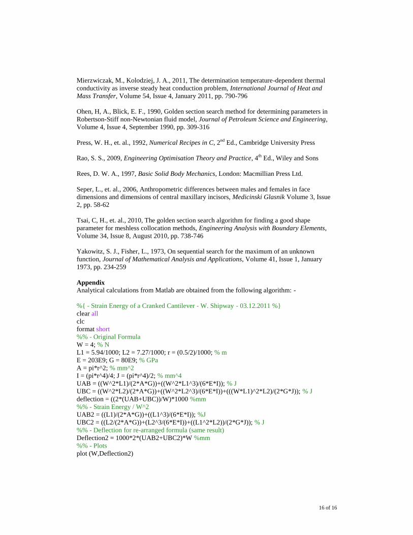
Appendix
Analytical calculations from Matlab are obtained from the following algorithm: -
%{ - Strain Energy of a Cranked Cantilever - W. Shipway - 03.12.2011 %} clear all clc format short %% - Original Formula W = 4; % N L1 = 5.94/1000; L2 = 7.27/1000; r = (0.5/2)/1000; % m E = 203E9; G = 80E9; % GPa A = pi*r^2; % mm^2 I = (pi*r^4)/4; J = (pi*r^4)/2; % mm^4 UAB = ((W^2*L1)/(2*A*G))+((W^2*L1^3)/(6*E*I)); % J UBC = ((W^2*L2)/(2*A*G))+((W^2*L2^3)/(6*E*I))+(((W*L1)^2*L2)/(2*G*J)); % J deflection = ((2*(UAB+UBC))/W)*1000 %mm %% - Strain Energy / W^2 UAB2 = ((L1)/(2*A*G))+((L1^3)/(6*E*I)); %J UBC2 = ((L2/(2*A*G))+(L2^3/(6*E*I))+((L1^2*L2))/(2*G*J)); % J %% - Deflection for re-arranged formula (same result) Deflection2 = 1000*2*(UAB2+UBC2)*W %mm %% - Plots plot (W,Deflection2)


