
www.iap.uni-jena.de
Design and Correction of Optical
Systems
Lecture 12: Optical system classification
2014-06-25
Herbert Gross
Summer term 2014

2
Preliminary Schedule
1 09.04. Basics Law of refraction, Fresnel formulas, optical system model, raytrace, calculation
approaches
2 16.04. Materials and Components Dispersion, anormal dispersion, glass map, liquids and plastics, lenses, mirrors,
aspheres, diffractive elements
3 23.04. Paraxial Optics Paraxial approximation, basic notations, imaging equation, multi-component
systems, matrix calculation, Lagrange invariant, phase space visualization
4 30.04. Optical Systems Pupil, ray sets and sampling, aperture and vignetting, telecentricity, symmetry,
photometry
5 07.05. Geometrical Aberrations Longitudinal and transverse aberrations, spot diagram, polynomial expansion,
primary aberrations, chromatical aberrations, Seidels surface contributions
6 14.05. Wave Aberrations Fermat principle and Eikonal, wave aberrations, expansion and higher orders,
Zernike polynomials, measurement of system quality
7 21.05. PSF and Transfer function Diffraction, point spread function, PSF with aberrations, optical transfer function,
Fourier imaging model
8 28.05. Further Performance Criteria Rayleigh and Marechal criteria, Strehl definition, 2-point resolution, MTF-based
criteria, further options
9 04.06. Optimization and Correction Principles of optimization, initial setups, constraints, sensitivity, optimization of
optical systems, global approaches
10 11.06. Correction Principles I Symmetry, lens bending, lens splitting, special options for spherical aberration,
astigmatism, coma and distortion, aspheres
11 18.06. Correction Principles II Field flattening and Petzval theorem, chromatical correction, achromate,
apochromate, sensitivity analysis, diffractive elements
12 25.06. Optical System Classification Overview, photographic lenses, microscopic objectives, lithographic systems,
eyepieces, scan systems, telescopes, endoscopes
13 02.07. Special System Examples Zoom systems, confocal systems
14 09.07. Further Topics New system developments, modern aberration theory,...
1. Overview
2. Achromates and apochromates
3. Collimators
4. Realy systems
5. Miscellaneous
6. Photographic lenses
7. Scan lenses
8. Lithographic lenses
9. Telescopes
10. Microscopic lenses
3
Contents

Field-Aperture-Diagram
0.20 0.4 0.6 0.80°
4°
8°
12°
16°
20°
24°
28°
32°
36°
NA
w
40°
micro
100x0.9
double
Gauss
achromat
Triplet
micro
40x0.6micro
10x0.4
Sonnar
Biogon
split
triplet
Distagon
disc
projection
Gauss
diode
collimator
projection
Petzval
micros-
copy
collimator
focussing
photographic
projection constant
etendue
lithography
Braat 1987
lithography
2003
Classification of systems with
field and aperture size
Scheme is related to size,
correction goals and etendue
of the systems
Aperture dominated:
Disk lenses, microscopy,
Collimator
Field dominated:
Projection lenses,
camera lenses,
Photographic lenses
Spectral widthz as a correction
requirement is missed in this chart

Throughput as field-
aperture product
Additional dimension:
spectral bandwidth
Classification: l-Lw-Diagram
Lw
l
Photography
Microscopy
Astronomy
LithographyInterferometer
lensmetrology lens
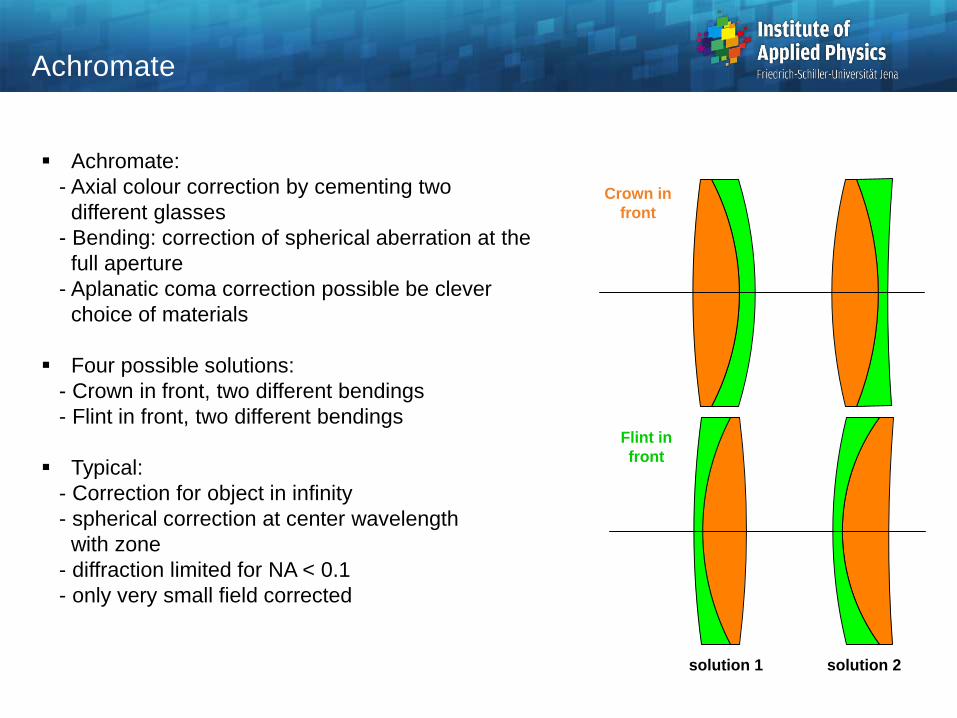
Achromate:
- Axial colour correction by cementing two
different glasses
- Bending: correction of spherical aberration at the
full aperture
- Aplanatic coma correction possible be clever
choice of materials
Four possible solutions:
- Crown in front, two different bendings
- Flint in front, two different bendings
Typical:
- Correction for object in infinity
- spherical correction at center wavelength
with zone
- diffraction limited for NA < 0.1
- only very small field corrected
Achromate
solution 1 solution 2
Crown in
front
Flint in
front
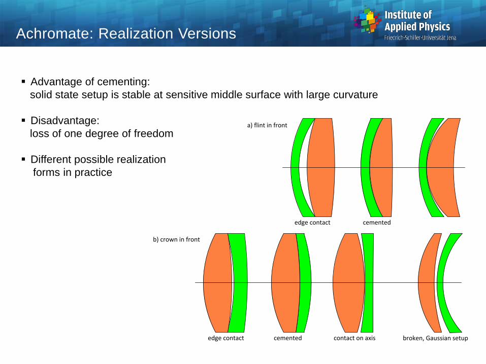
Achromate: Realization Versions
Advantage of cementing:
solid state setup is stable at sensitive middle surface with large curvature
Disadvantage:
loss of one degree of freedom
Different possible realization
forms in practice
edge contact cemented
a) flint in front
edge contact cemented contact on axis broken, Gaussian setup
b) crown in front

Achromate
Achromate
Longitudinal aberration
Transverse aberration
Spot diagram
rp
0
486 nm
587 nm
656 nm
0.1 0.2
s'
[mm]
1
axis
1.4°
2°
486 nm 587 nm 656 nm
l = 486 nm
l = 587 nm
l = 656 nm
sinu'
y'

9
Axial Color Correction
(c) Apochromat
FK51, KZFS11, SF6
(b) Achromat
BK7, F2
(a) Single element
BK7
System
Improvement
1/20
Improvement
1/100
Chromatic focal shift
656 nm
656 nm
656 nm
436 nm
436 nm
436 nm
Ref.:H. Zuegge

Choice of at least one special glass
Correction of secondary spectrum:
anomalous partial dispersion
At least one glass should deviate
significantly form the normal glass line
Axial Colour : Apochromate
656nm
588nm
486nm
436nm1mm
z0-0.2mm
z-0.2mm
2030405060708090
N-FK51
N-KZFS11
N-FS6
(1)
(2)
(3)
(1)+(2) T
PgF
0,54
0,56
0,58
0,60
0,62
n
10

Conventional achromate: strong bending of image shell, typical
Special selection of glasses:
1. achromatization
2. Petzval flattening
Residual field curvature:
Combined condition
But usually no spherical correction possible
'
111
2
2
1
1
12 fnnRptz
nn
nn
'3.1 fRptz
New Achromate
perfect
image
plane
Petzval
shell
y'
f
RP
mean
image shell
2
1
2
1
n
n
n
n
02
2
1
1 n
n
FF
02
2
1
1 n
F
n
Fn
n
selected crown glass
line of solutionfor flint glass
11

Collimation
D
source
G/2divergence
f
u
Collimating source radiation:
Finite divergence angle is reality
Geometrical part due to finite size :
Diffraction part:
Defocussing contribution to divergence
f
DG
DD
l
uf
zsin
2

Collimator Optics
spherical
coma
astigmatism
curvature
distortion
1 2 3 sum
-0.1
0
0.1
-5
0
5
-2
0
2
-2
0
2
-4
-2
0
2
4
4
Monochromatic doublet
Correction only spherical and coma:
Seidel surface contributions
Limiting : astigmatism and curvature
Enlarged aperture : meniscus added

Relay Systems: Achromate
Large residual aberrations:
1. Astigmatism
2. Field curvature
-1.5 0 1.5
0.5
1.0
a) spherical aberration
z
[mm]
yp
/ ypmax
-2.0 0 2.0
0.5
1.0
b) astigmatic field curves
z
[mm]
y' / y'
maxsagtan
-1.0 0 1.0
0.5
1.0
c) distortion
[%]
y' / y'
max
656 nm
546 nm
486 nm
435 nm

Relay Systems: Achromate with Field Lens
Correction comparable
Better fit of pupil
-1.5 0 1.5
0.5
1.0
a) spherical aberration
z
[mm]
yp
/ ypmax
-2.0 0 2.0
0.5
1.0
b) astigmatic field curves
z
[mm]
y' / y'
maxsagtan
-1.0 0 1.0
0.5
1.0
c) distortion
[%]
y' / y'
max
656 nm
546 nm
486 nm
435 nm
-1.5 0 1.5
0.5
1.0
a) spherical aberration
z
[mm]
yp
/ ypmax
-2.0 0 2.0
0.5
1.0
b) astigmatic field curves
z
[mm]
y' / y'
maxsag
tan
-1.0 0 1.0
0.5
1.0
c) distortion
[%]
y' / y'
max
656 nm
546 nm
486 nm
435 nm

Relay Systems: More Complicated Systems
Improved performance with more lenses
In particular better color correction
Magnification m = 0.2 -0.5 0 0.5
1.0
a) spherical aberration
z
[mm]
yp
/ ypmax
-0.1 0 0.1
0.5
1.0
b) astigmatic field curves
z
[mm]
y' / y'
max
656 nm
546 nm
486 nm
solid: tan
dashed: sag
0.5
486 nm
587 nm
656 nm
y/ymax
b) field curvature
T S
0.1-0.05 0 0.05
s'
[mm] -0.05 0
T S T S y/ymax
c) distortion
[%]
a) spherical aberration
-0.2 0 0.2
0.5
1.0
z
[mm]
yp
/ ypmax

Relay Systems: 4f-Systems
Basic system with achromates
Split achromates
-1.5 0 1.5
0.5
1.0
a) spherical aberration
z
[mm]
yp
/ ypmax
-2.0 0 2.0
0.5
1.0
b) astigmatic field curves
z
[mm]
y' / y'
max
sag
tan
-1.0 0 1.0
0.5
1.0
c) distortion
[%]
y' / y'
max
656 nm
546 nm
486 nm
435 nm
-1.5 0 1.5
0.5
1.0
a) spherical aberration
z
[mm]
yp
/ ypmax
-2.0 0 2.0
0.5
1.0
b) astigmatic field curves
z
[mm]
y' / y'
max
sagtan
-1.0 0 1.0
0.5
1.0
c) distortion
[%]
y' / y'
max
656 nm
546 nm
486 nm
435 nm

Double telecentric: magnification
Wave transport: phase is invariant
use in phase imaging
Use in Fourier-optical setups or pupil transfer systems
final
plane
starting
plane
f1
f1
f2
f2
d'd
1
2
f
f
yxEyxE ,
1),('
Relay Systems: 4f-Systems

Relay Systems: Periscope
Major parts:
1. Eyepiece
2. Relay system, several stages
3. Objective
4. Turnable prism
eyepiece
objective
field lens
1. image
1. relay system
2. relay system
2. image
3. relay system

Relay Systems: Endoscopes
Different subsystems:
Differences in performance, complexity, distance, weight
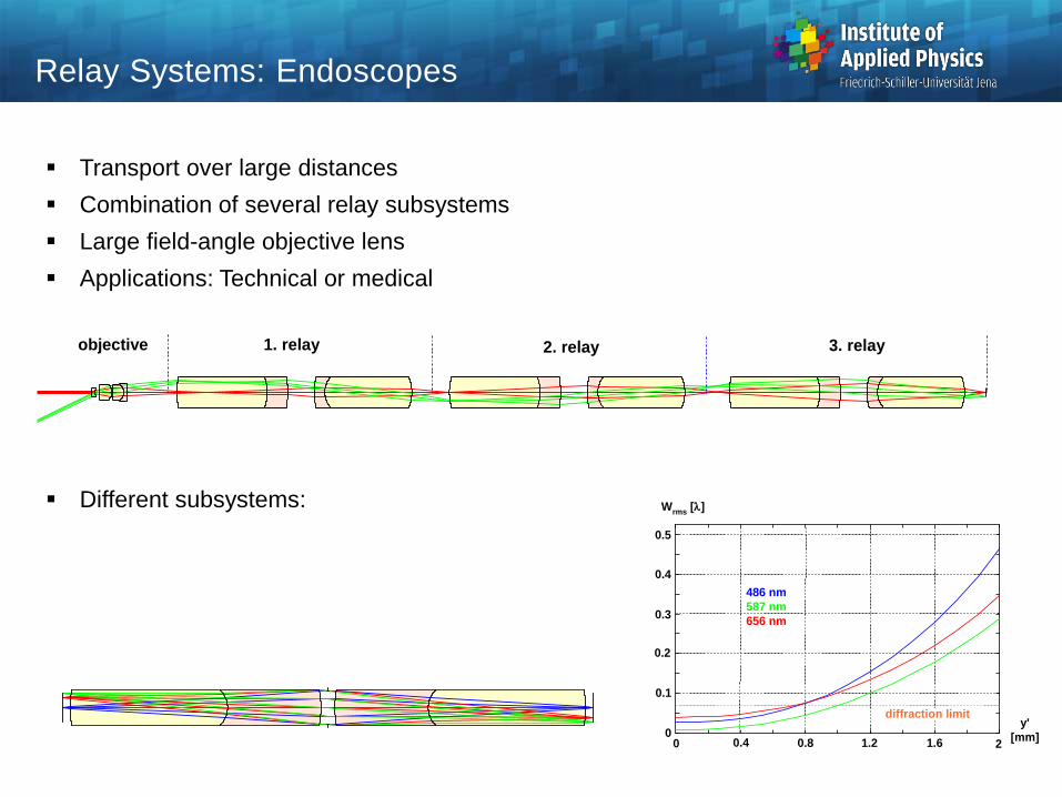
Relay Systems: Endoscopes
Transport over large distances
Combination of several relay subsystems
Large field-angle objective lens
Applications: Technical or medical
Different subsystems:
objective 1. relay 2. relay 3. relay
0.5
486 nm
587 nm
656 nm
0.4
00 0.4
Wrms
[l]
0.8 1.2 21.6
y'
[mm]
0.3
0.2
0.1
diffraction limit
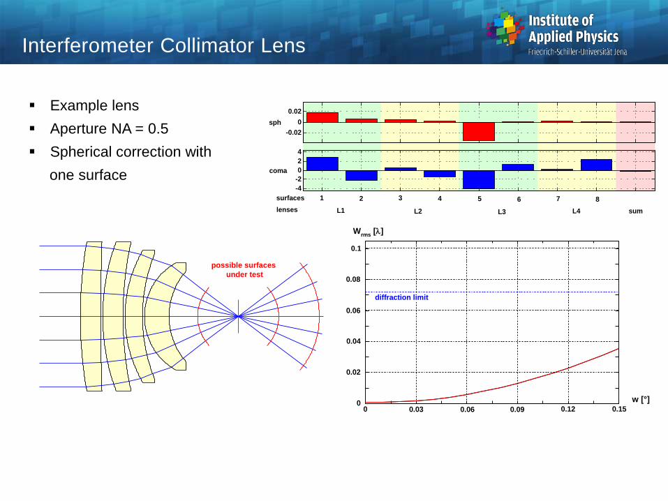
Interferometer Collimator Lens
Example lens
Aperture NA = 0.5
Spherical correction with
one surface
possible surfaces
under test
Wrms
[l]
0.1
0.08
0.06
0.04
0.02
00 0.03 0.06 0.09 0.150.12
w [°]
diffraction limit
-0.02
0
0.02
sph
-4
-2
0
2
4
coma
surfaces
sumL1 L2 L3 L4lenses
1 2 3 4 5 6 7 8

Beam Guiding Systems
= 5
= 5
= 4
= 50
= 4
a)
b)
c)
d)
e)
adjustment
Transport of laser light over large
distances
Adaptation of beam diameter
Solutions :
Telescopes of Kepler or Galilei type

Families of photographic lenses
Long history
Not unique
Classification
Singlets
Landscape
Achromatic
Landscape
Petzval, Portrait
Petzval,Portrait flat R-Biotar
Petzval
Petzval
Projection
Quasi-Symmetrical Angle
Pleon
Panoramic
Lens
Extrem Wide Angle
Fish Eye
VivitarRetrofocus II
Wide Angle Retrofocus
Distagon
SLR
Flektogon
Retrofocus
PlasmatKino-Plasmat
Ultran
Noctilux
Quadruplets
Double Gauss
Biotar / Planar
Double Gauss II
Celor
Compact
Special
Plastic Aspheric
II
IR Camera Lens
Catadioptric
UV Lens
Plastic
Aspheric I
Telephoto
Telecentric II
Telecentric I
Super-Angulon
Hologon
MetrogonTopogon
Hypergon
Pleogon
Biogon
Triplet
Triplets
Inverse Triplet
Heliar Hektor
Pentac
Sonnar
Ernostar II
Less Symmetrical
Ernostar
Orthostigmatic
Symmetrical Doublets
Periskop
Rapid
Rectilinear
Aplanat
Dagor
Dagor
reversed
Angulon
Protar
AntiplanetUnar
Quasi-Symmetrical Doublets
Tessar
Tessar
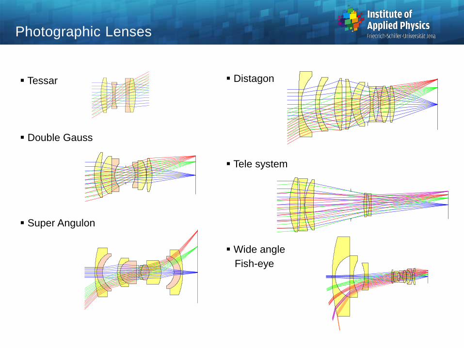
Double Gauss
Super Angulon
Photographic Lenses
Distagon
Tele system
Wide angle
Fish-eye

Example lens 2
Distagon
Retrofocus Lenses
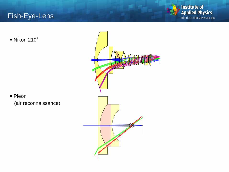
Nikon 210°
Pleon
(air reconnaissance)
Fish-Eye-Lens

Zoom lens
Three moving groups
Zoom Lens
e)
f' = 203 mm
w = 5.64°
F# = 16.6
d)
f' = 160 mm
w = 7.13°
F# = 13.7
c)
f' = 120 mm
w = 9.46°
F# = 10.9
b)
f' = 85 mm
w = 13.24°
F# = 8.5
a)
f' = 72 mm
w = 15.52°
F# = 7.7
group 1 group 2 group 3

Handy Phone Objective lenses
Examples
Ref: T. Steinich
US 7643225L = 4.2 mm , F'=2.8 , f = 3.67 mm , 2w=2x34°
US 6844989L = 6.0 mm , F'=2.8 , f = 4.0 mm , 2w=2x31°
EP 1357414L = 5.37 mm , F'=2.88 , f = 3.32 mm , 2w=2x33.9°
Olympus 2L = 7.5 mm , F'=2.8 , f = 4.57 mm , 2w=2x33°
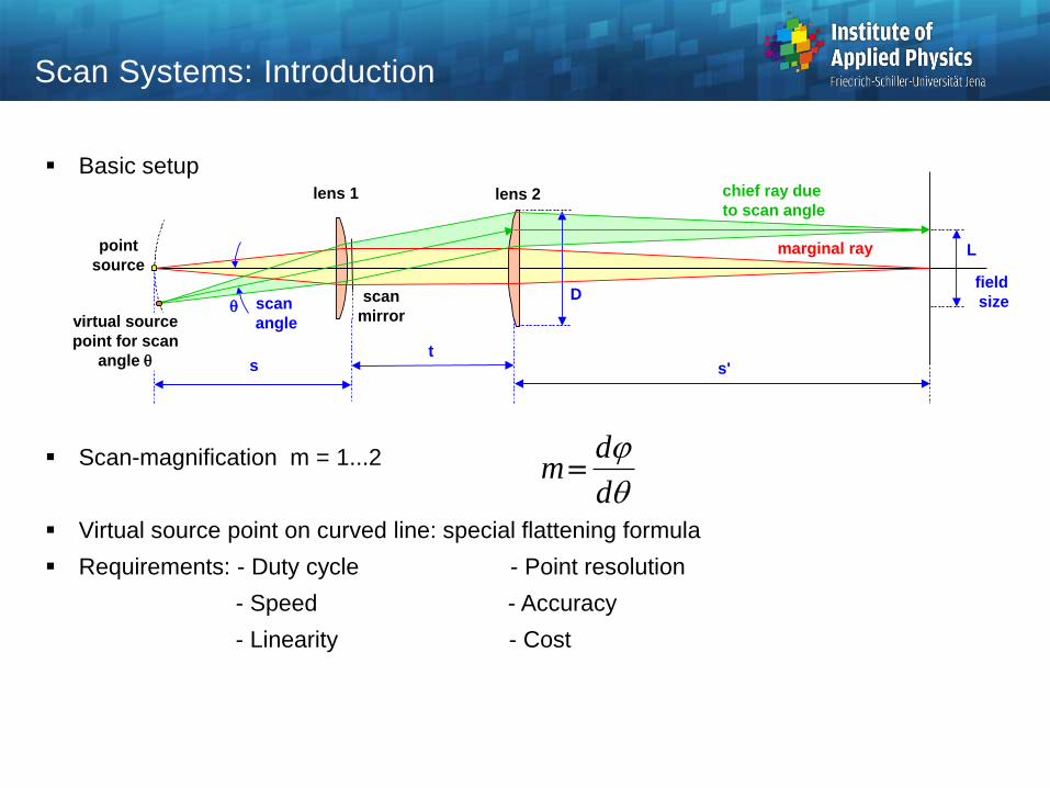
Scan Systems: Introduction
Basic setup
Scan-magnification m = 1...2
Virtual source point on curved line: special flattening formula
Requirements: - Duty cycle - Point resolution
- Speed - Accuracy
- Linearity - Cost
d
dm
point
source
lens 1 lens 2
scan
mirror
marginal ray
chief ray due
to scan angle
D
L
s't
s
field
sizescan
anglevirtual source
point for scan
angle

Scan Systems: Introduction
Scan resolution:
Number of resolvable points in the field of view
corresponds to angle resolution
Information capacity:
1. Resolvable points
2. Speed of scanning
l
max2 ExP
Airy
D
D
LN
log
log v
angle
resolution
scan speed
growing scan
capacity
acoustic optical modulator
polygon
mirror
galvo
scanner
holographic
scanner
electro
optical
modulator
resonant
galvo
scanner

Scan System
Non-telecentric
Scan angle 2x30°
Monochromatic
F--corrected
a) standard distortion
-10%
1
0.5
y/ymax
b) f--distortion
0 10% -0.2% 0 0.2%
1
0.5
y/ymax
0
0.1
0.08
0.06
0.04
0.02
0
Wrms
[l]
15° 30°
c) wave aberration
0° 5° 10°
20°
15°
24° 28° 30.4°

Scan Systems: Introduction
Deflecting components
allows a field scan
Mostly rotating mirrors
Pre-objective scanning
Post-objective scanning
y
scan
objective
lens
rotating scan
mirror
scan
angle image
plane
y
scan
mirror
scan lens
image
surface

Deflecting Components: Polygon Mirrors
Rotating mirror with plane facets
Pyramidal
Prismatic
scan
line
objective
lens
prismatic
polygon
scan line
pyramidal
polygon objective
lens

Evolution of Projection lenses
Growing NA and field of view:
Increasing size of objective lenses
Problems with correction, homogeneity, material cost, thermal effects
Technological steps: aspherical surfaces, immersion, catadioptric designs
0.5 0.7 0.9 1.1 1.3 1.5 1.7
Volume
[a.u.]
NA
pure
spherical
immersion
high index
hypothetical
n = 1 n H20
(193nm)
0
0.2
0.4
0.6
0.8
1
aspherical
strong
aspherescatadioptric
0.00
0.20
0.40
0.60
0.80
1.00
1.20
0.80 0.90 1.00 1.10 1.20 1.30 1.40 1.50 1.60 1.70
Volume [a.u.]
refractive
folded catadioptric
HI
inline catadioptric
-
NA
HI
expectation
hyper-NA
n = 1 nH2O
(193 nm)
design
progress

Size Reduction by Aspheres
Considerable reduction
of length and diameter
by aspherical surfaces
a) NA = 0.7
spherical
b) NA = 0.8
spherical
c) NA = 0.8
aspherical
d) NA = 0.9
aspherical
-13%
-9%

Fundamental System Groups
Principal layout of a lithographic system
beam steering
mirror
pupil
shaping
integrator rod
reticle
wafer
laser
projection
lens
rema relay lenshomogenizer
diffuser
beam guiding
diameter
adaptation
axicon
zoom

Ref: W. Kaiser
Development of Stepper Lenses

Moores Law
Historical development of shrinking feature size
Moores law: factor 2 every two years
EUV
ArF 193 immersion
ArF 193
resolution
[mm]
1.0
0.7
0.5
0.35
0.25
0.18
0.13
0.1
0.07
0.05
0.035
1985 1990 1995 2000 2005 2010year
g-line 436
i-line 365
KrF 248
Intel 48633 Mhz
Pentium
Pentium II
Pentium III
Pentium IV
FutureProcessors
Processors:
66- 100 Mhz-
300 Mhz
600 Mhz
1-2 Ghz-
3 Ghz
4-10 Ghz-

Ref: Carl Zeiss AG
Lithographic Lens in Reality

Lithographic Lens Example Layouts
reticle
mask
stop
mask
reticle
stop
1. relay group
2. relay group
reticle
wafer
mirror
with relay
group
intermediate
image

Lithographic Optics
EUV a-Tool 2008

Lithographic Optics
H-Design

Lithographic Optics
I-Design

Lithographic Optics
X-Design

Development of Lithographic Lenses
b) Refractive spherical systems
a) Early systemsg) EUV
mirror
systems
M1
M3
M2
M4
M4
M3
M1
M2
M5
M6
M1
M2
M3
M4
M5
M6
M8
M6
c) Refractive with aspheres and immersion
d) Catadioptric cube systems
e) Multi-axis catadioptric systems
f) Uni-axis catadioptric systems

Field Flatness
Principle of multi-bulges to
reduce Petzval sum
Seidel contributions show principle
-0.2
0
0.2
10 20 30 40 6050
1. bulge 2. bulge 3. bulge1. waist 2. waist
one waist two waists
Petz Petz
1 1
rn
n fp k kk
'

Projection Processing Modes
Different process modes:
1. Full field
2. Scanning
3. Step and repeat
a) Full wafer projection
Reticle
Lens
Wafer
b) Full wafer scanning
Reticle
Lens
Wafer
c) Step and repeat
Reticle
Lens
Wafer
d) Step and scan
Reticle
Lens
Wafer

Resolution
Lateral resolution (CD)
k1 = 0.25 ... 0.5
Axial resolution
High NA :
Influence:
Wavelength and NA
Diagram : k1 = 0.36, k2 = 0.28
0.85
0.75
0.65
0.55
0.45
0.35
0.95 = NA
z [mm]
10-1
10-1
100
x
[mm]
405
l = 157
193
248
365
NAkx 0
1
l
2
02
NA
nkz
l
2
)/(11 2
2
02
nNA
NA
nkz
l

Basic Refractive Telescopes
Kepler typ:
- internal focus
- longer total track
- > 0
Galilei typ:
- no internal focus
- shorter total track
- < 0
Telescopepupil
intermediatefocus
Eyepiece
Eye pupil
telescope focal length fT
eyepiece focal length f
ETelescopepupil
Eye pupil
telescope focal length fT
eyepiece focal length f
E
a) Kepler/Fraunhofer
b) Galilei
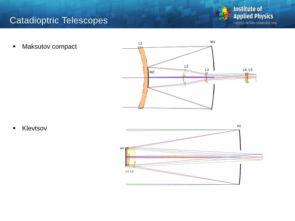
Catadioptric Telescopes
Maksutov compact
Klevtsov
M1
M2
L1
L2L3 L4, L5
M1
L1, L2
M2

Astronomical Telescope
Primary and
secondary mirror

Four-Mirror Schiefspiegler Telescopes
Solution Variants A
B
D
E
F
GH

Catadioptric Telescopes
Schmidt Telescope
- Aspherical corrector plate
- Residual chromatical aberrations
- Achromatic corrector plate possible
Image
Primary mirror
r = 2f
f
Stop
M1
Correctorplate
Stop
M1
focal plane(curved)
N-BK7N-F2
primary mirror
focus
corrector plate
y
r
a
marginal rays
field

Evolution of Eyepiece Designs
Monocentric
Plössl
Erfle
Von-Hofe
Erfle diffractive
Wild
Erfle type(Zeiss)
BerteleScidmore
Loupe
Erfletype
Bertele
Kellner
Ramsden
Huygens
Kerber
König
Nagler 1
Nagler 2
Bertele
Aspheric
Dilworth

instrument
pupil
x'
z'
e x
s'
F'
f1
f2
field
lens
intermediate
image
stopeye
lens
eye
pupil
Eyepiece: Notations
Field lens reduces chief ray
height
Eye lens adapts pupil diameter
Matching of
1. Field of view
2. Pupil diameter
3. Pupil location
Eye relief :
- distance between last lens surface and eye cornea
- required : 15 mm
- with eyeglasses : 20 mm
Pupil size: 2-8 mm

Kellner Eyepiece
Corresponds to Ramsden type
Field lens moved
Eye lens achromatized
-1.000 0.000 1.000
0.250
0.500
0.750
1.000
LONGITUDINALSPHERICAl ABER.
DIOPTER
-3.000 0.000 3.000
2.625
5.250
7.875
10.500
tan sag
ASTIGMATICFIELD CURVES
DIOPTER
-20.00 0.00 20.00
2.625
5.250
7.875
10.500
DISTORTION
Distortion (%)
0°
10°
20°
24°
20
arc
min

Abbe Orthoscopic Eyepiece
Distortion corrected
General problems with eyepieces:
- remote eye pupil
- typical eye relief 22 mm
-1.000 0.000 1.000
0.250
0.500
0.750
1.000
LONGITUDINALSPHERICAl ABER.
DIOPTER
-3.000 0.000 3.000
2.000
4.000
6.000
8.000
tan sag
ASTIGMATICFIELD CURVES
DIOPTER
-20.00 0.00 20.00
2.000
4.000
6.000
8.000
DISTORTION
Distortion (%)
0°
10°
18°
20 a
rcm
in

Application Fields of Microscopy
Ref: M. Kempe
Cell biology
biological development
toxicology,...
Biomedical basic
research
Material
research
Research
Medical
routine
Pharmacy
semiconductor inspection
semiconductor manufacturing
Industrial
routine
Routine
applications
Microscopy
Micro system technology
geology
polymer chemistry
Pathology
clinical routine
forensic,...
Microscopic surgery
ophthalmology

Image Planes and Pupils
Principal setup of a classical optical microscope
Upper row : image planes
Lower row : pupil planes
Köhler setup
source
collector condenser objective eyepiece eyetube lens
eye
pupil
exit pupil
objective
aperture
stopfield
stop
object intermediate image image

Microscope with Infinite Image Setup
Basic microscopic system with infinite image location and tube lens
Magnification of the first stage:
Magnification of the complete setup
Exit pupil size
eyeobj
tubemicro
f
mm
f
fm
250
obj
tubeobj
f
fm
obj
obj
objExPm
NAfNAfD
2'2
marginal
ray
eyepiece
chief ray
w'
intermediate
imageobjective
lens
object
eye
tube length t
h'
h
fobj
w
pupil tube lens
s1
feye
eye
pupil

Upright-Microscope
Sub-systems:
1. Detection / Imaging path
1.1 objective lens
1.2 tube with tube lens and
binocular beam splitter
1.3 eyepieces
1.4 optional equipment
for photo-detection
2. Illumination
2.1 lamps with collector and filters
2.2 field aperture
2.3 condenser with aperture stop
eyepiece
photo
camera
tube lens
objective
lens
lamp
lamp
collector
collector
condensor
intermediate
image
binocular
beamsplitter
object
film plane
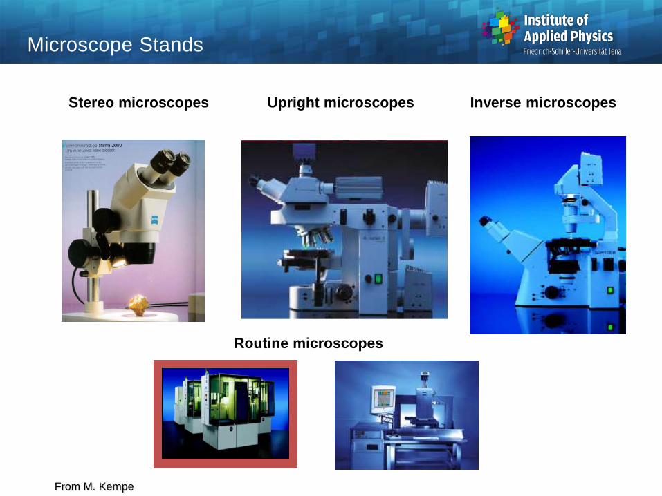
Stereo microscopes Upright microscopes Inverse microscopes
Routine microscopes
From M. Kempe
Microscope Stands
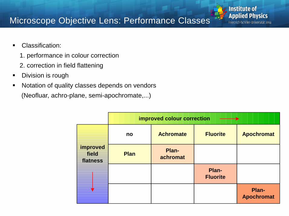
Microscope Objective Lens: Performance Classes
Classification:
1. performance in colour correction
2. correction in field flattening
Division is rough
Notation of quality classes depends on vendors
(Neofluar, achro-plane, semi-apochromate,...)
improved
field
flatness
improved colour correction
Achromate
Plan-
Apochromat
Fluorite Apochromatno
PlanPlan-
achromat
Plan-
Fluorite

Microscope Objective Lens: Structure
Typical parts of lens structure for high NA-objective lenses
Separation of the lens setup in 3 major sections
afront part :
1. spherical aberration : only small
2. coma : only small
3. astigmatism : only small
4. curvature : only small
b
middle part :
1. spherical aberration : correction
2. color : correction
3. coma : correction
rear part :
1. curvature : correction
2. astigmatism : correction
3. color : correction
c

Microscope Objective Lens Types
Medium magnification system
40x0.65
High NA system 100x0.9
without field flattening
High NA system 100x0.9
with flat field
Large-working distance
objective lens 40x0.65

Microscope Objective Lens: Correcting lens
Floating element to
adjust and correct
spherical aberration
Applications:
1. different thickness values
of cover glass
2. index mismatch at
the sample
floating
element
+1.80 mm
+1.63 mm
0.7 mm
cover
slide
air distance
1.2 mm
1.7 mm
0 mm
4.46
mm
3.99
mm
3.66
mm
3.32
mm
+2.04 mm

Microscope Objective Lens: Pupil
Object space telecentric
Real rear stop is not
defining the pupil
Collimated outgoing
beam
Exit pupil usually
not accessible
object
plane
objective
lens
rear stop
exit pupil
marginal ray
chief ray
telecentric,
entrance pupil infinity
y'p
u
f'f'
chief
ray
exit
pupil
rear
stopobject
plane
pupil

Illumination Optics: Overview
Instrumental realizations
a) incident illumination
bright fieldb) incident illumination
dark fieldc) transmitted illumination
bright field
d) transmitted illumination
dark field
ring
mirrorobservation
illumination
object
plane
ring
mirror
objective
lens
object
plane
observation
illumination
observation
ring
condenser
object
plane
illumination
condenser
object
plane
observation
illumination

Stereo Microscope
Telescopic setup : common main objective lens
View along the axis
eyepiece
tube
system zoom
system object
plane
eye
common
axis
stereo
angle
common
objective
lens
left
imaging
channel
right
imaging
channel
possible
illumination
channels


