
Supporting smart urban growth: Successful Investing in Density FULL REPORT
Authors and Contributors:
Professor Kathy Pain, Department of Real Estate & Planning, University of Reading
Daniel Black, Daniel Black & Associates
Dr Jon Blower, Institute for Environmental Analytics, University of Reading
Professor Sue Grimmond, Department of Meteorology, University of Reading
Dr Alistair Hunt, Department of Economics, University of Bath
Dr Stanimira Milcheva, Department of Real Estate & Planning, University of Reading
Dr Ben Crawford, Department of Meteorology, University of Reading
Nick Dale, Department of Economics, University of Bath
Dr Sam Doolin, Institute for Environmental Analytics, University of Reading
Dr Senjuti Manna, Department of Real Estate & Planning, University of Reading
Dr Shuai Shi, Department of Real Estate & Planning, University of Reading
Dr Ruth Pugh, Department of Real Estate & Planning, University of Reading
& employment infrastructure
people, skills, capital, firms, knowledge
Coordinated… governance infrastructure & green/blue infrastructure
planning & policy spanning functional urban area

2
Acknowledgements
Project sponsors
Project advisor
Project Steering Group
Project Director

3
Project Team
Special Thanks

Table of Contents
Introduction ................................................................................................................................ 2
The two-phase method ......................................................................................................... 2
Key findings ................................................................................................................................ 8
Successful investing in density .........................................................................................33
Supporting smart urban growth .....................................................................................38
Technical annexes ..................................................................................................................46
2
Successful investing in density - Implications for investment and policy
decision-making
Introduction
This research commissioned by Urban Land Institute (ULI) and New Climate Economy (NCE),
supported by a steering group of global real estate and infrastructure fund managers and investors,
set out to objectively evaluate the impact of investment in compact, connected urban development
on returns1 for real estate investors, and the implications for carbon (CO2) emissions and
infrastructure cost per resident for the public sector. The scope of the research is global but with a
focus on comparing and contrasting quantitative data on cities in OECD nations with that for cities in
fast growing developing world regions.
The results of the two-phase study undertaken by a multi-disciplinary research team led by
Professor Kathy Pain of the Henley Business School at the University of Reading, are intended to help
inform private and public sector decision-making on the ways in which smarter infrastructure
investment in ‘good density’ can help to support investment returns while reducing CO2 emissions.
The two-phase method
Phase I
In the first phase of the research, the relationship between good density (defined by ULI as mixed
use, connected, planned, cohesive, liveable, spacious, flexible, design, green and appropriate, Clark
and Moir, 2015) and urban form characteristics and real estate investment returns, was
investigated. A summary of the findings is presented in the Phase I report.
An interdisciplinary literature review was conducted to generate a shortlist of urban form
characteristics linked to good density using inductive and deductive approaches, and to identify
relevant data for incorporation in Phase II quantitative analysis.2 Works reviewed extended beyond
the urban design and planning literature to encompass 65 international peer-reviewed academic
journals and reports published by official bodies and think tanks, including the ULI and NCE. From
the literature review, six core urban form characteristics relevant for good density were identified.
1 The return on investment (ROI) is a critically important property attribute driving real estate investment. 2 The framework for identifying relationships between good density and urban form characteristics was developed by conducting an extensive systematic design and planning literature search with advice from external experts, to establish patterns of association (Inductive approach) and by drawing on established knowledge and theories in the literature of other relevant disciplines to test those patterns (deductive approach) (McGhee, et al., 2007).

3
Core characteristics of urban form
identified from literature review
Clustering Structure
Clustering patterns within cities and at city-
region scale determine the level of volume
of carbon-generating traffic movement, i.e.
travel for work, business meetings, leisure,
and agglomeration economies / inward
investment.
Economic/Employment Infrastructure
Connectivity to and concentration of
foreign investment, quality value adding
jobs, labour, skills, diversity and innovation
capacity all feature in creating a strong,
resilient city economy.
Built Infrastructure
Elements of built infrastructure that impact
on good density are mixed use planning,
technological and design quality, and
amenity at property level and urban
landscape scale.3
Public Transport Infrastructure
The capacity of public transportation
serving a city, accessibility to the public
transport network and the quality of
services.
Green/Blue Infrastructure
The capacity, quality and accessibility of
blue and green infrastructure within cities
contribute to ecological sustainability,
human health and well-being.
Governance Infrastructure
Appropriate governance underpins good
density. It needs to be spatially aware,
integrated horizontally and vertically and to
have a well-developed, responsible public-
private investment strategy.
3 Due to the high importance of public transport infrastructure in supporting good density noted in the literature reviewed and a lack of globally comparable comprehensive public infrastructure costs data, priority was given to transport infrastructure costs for four city case studies identified in Phase II of the research.

4
Global indices relevant for the six urban form characteristics underpinning good density were then
identified and evaluated to establish the robustness and comparability of their underlying data. 12
indices4 were finally incorporated in quantitative analysis in Phase II of the study to examine the
significance of good density for real estate investment returns.
Notes:
(1) AoUE data on urban extent and built up area density are based on population per hectare and are together representative of compact development, as opposed to simply city size.
(2) GaWC business and financial services shed light on commercial office occupation and functional density, complementing the AoUE focus on urban residential density (population per hectare).
(3) JLL transparency data are taken from an index comprised of national metrics. (4) AoUE satellite data on walkability are based on accurate metrics available from remote
photography however the quality of walking route, e.g. whether a route is safe and enjoyable to walk is unknown.
(5) AoUE data on built form, urban extent and open space ratio (i.e. size of block or open space) indicate the different spatial patterns of density within a given built up area, however building uses and heights are not surveyed. The GaWC data indicate commercial office use and are a proxy for central business district building heights.
(6) ARCADIS green environment is a composite city ranking of indicators relevant for good density that draws on a number of reputable individual sources (see Technical Annex IB).
4 For descriptions of the indices see Technical Annex IB.

5
Phase II
The second phase of the project focused on quantitative analysis of relationships between good
density indicators relevant for the urban form characteristics and real estate investment returns,
and their implications for CO2 emissions and infrastructure costs.
Semi-structured interviews with ULI real estate industry project steering group members were first
conducted to provide qualitative insights into fund management and investor interest in supporting
good density, how good density is currently incorporated in private sector decision making, and to
help with the identification of additional relevant data.5 A summary of the interview findings is
included in Technical Annex II to this report.
To better capture the different dimensions of the real estate market in response to fund
management and investor interest in not only returns but investment value and performance, three
data sources were used in analysis. The conventional real estate yields6 data, supplied by CBRE,
have been used to calculate returns. We used data supplied by Cushman & Wakefield (CW) on
capital value and rents for European markets. Real Capital Analytics (RCA) data on global cross-
border real estate portfolio capital flows7 were also incorporated. Following the standard
methodology applied in the academic real estate literature, due to annual point-in-time volatility of
real estate performance, average performance has been used to calculate relationships with good
density characteristics (see for example, Lizieri et al., 2012). Data available to the research team for
all three sources were for the time period since 2008
CBRE data are on a quarterly basis for 63 cities internationally.8 CW rental and yield data for a sub-
set of 27 European cities allowed the incorporation in analysis of data for prime retail as well as
office markets.9 In both cases, data are based on local appraisal information. RCA global data for
commercial office property based on transactions values were therefore also incorporated in
analysis to shed light on cities that are attracting major property investment flows.
Table 1 summarises the number of cities for each variable for which investment and good density
data were available. Due to some cities, and thereby metrics, having large proportions of missing
data, and a lack of comparable time-series data, analysis is limited in terms of formal econometric
modelling. Also for several good density variables (tourism, transparency, green environment, and
innovation) indices provide only the relative rank of cities globally. As a result, we do not report
results from regression analysis but use rank correlation analysis instead based on the most recent
data from 2016 indices. For the cases in which more than 50 observations are available, we ran
univariate and multivariate regressions as a robustness check for our baseline correlation results.
Overall, we did not find that using regression analysis leads to different conclusions. It is important
5 See Technical Annex II for details of the interview research ethics procedure, information sheet and signed consent form, and the questionnaire proformas. 6 The yield on a property is the annual return on a capital investment as a percentage of the capital value. 7 Flows of capital into real estate – see Lizieri et al., 2012. 8 Japanese cities are not included in the CBRE data base and were therefore not able to be included in the analysis. 9 Residential markets relevant for good density require research in follow up studies, e.g. non-commercial residential property important for affordable housing supply and robust comparable data on the commercial residential market required for global analysis.

6
to note that this methodology does not account for causality. The relationship between variables
has been determined using the Spearman’s rank-based correlation coefficient (Spearman. 1904)
given as:
,
cov( , )i j
i j
i j
v v
(1)
with ,i j denoting the Pearson correlation coefficient, cov( , )i jv v the covariance between rank
variable iv and rank variable jv and i being the standard deviation of rank variable iv and j
being the standard deviation of rank variable jv . The correlation coefficients are calculated for a
cross section of cities’ data. The year of the good density data varies for individual indices but for
most variables it is based on data since 2014.
The data sources used in the analysis together with data and analytical challenges and limitations,
and validity tests run, are detailed in Technical Annex I to this report.
Table 1 Number of observations (N) for each variable.
Variable N
Returns after 2008 63
Real estate investment flows 63
Business services 63
Financial services 59
Innovation 63
Low unemployment 63
Low crime 62
Green environment 37
Transparency 57
Urban extent density 50
Built up area density 61
Open space ratio 28
Walkability ratio 28
Tourism 28
The results presented in this report are for global and European levels of analysis. Additional insights
are presented for selected cities in mature economies (London, New York and Hong Kong) and
developing economies (Beijing, Mumbai and Warsaw) and for four case study cities (London, New
York, Hong Kong and Zürich) identified on the basis of interesting global and European correlation
results.
Moreover, a prototype working tool for city mapping and visualization has been developed to
demonstrate how the present analysis could be taken forward to assist private and public sector
investment decision making. Screenshots illustrating the tool interface for the London case study
shown in Exhibits 1 to 4, illustrate how in-depth relationships between real estate investment and

7
urban form characteristics important for good density can be informed by the incorporation of
detailed local information on potential confounding variables not revealed in global analysis.10
10 Confounding variables are variables not controlled for in analysis. Local confounding variables reflecting spatial heterogeneity could compromise the validity of global correlations (see Technical Annex !B).
8
Key findings
Global insight – Commercial offices
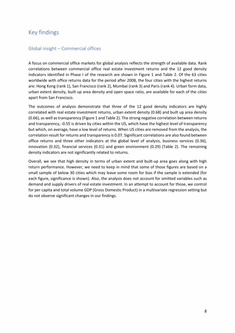
A focus on commercial office markets for global analysis reflects the strength of available data. Rank
correlations between commercial office real estate investment returns and the 12 good density
indicators identified in Phase I of the research are shown in Figure 1 and Table 2. Of the 63 cities
worldwide with office returns data for the period after 2008, the four cities with the highest returns
are: Hong Kong (rank 1), San Francisco (rank 2), Mumbai (rank 3) and Paris (rank 4). Urban form data,
urban extent density, built up area density and open space ratio, are available for each of the cities
apart from San Francisco.
The outcomes of analysis demonstrate that three of the 12 good density indicators are highly
correlated with real estate investment returns, urban extent density (0.68) and built up area density
(0.66), as well as transparency (Figure 1 and Table 2). The strong negative correlation between returns
and transparency, -0.55 is driven by cities within the US, which have the highest level of transparency
but which, on average, have a low level of returns. When US cities are removed from the analysis, the
correlation result for returns and transparency is 0.07. Significant correlations are also found between
office returns and three other indicators at the global level of analysis, business services (0.36),
innovation (0.32), financial services (0.31) and green environment (0.29) (Table 2). The remaining
density indicators are not significantly related to returns.
Overall, we see that high density in terms of urban extent and built-up area goes along with high
return performance. However, we need to keep in mind that some of those figures are based on a
small sample of below 30 cities which may leave some room for bias if the sample is extended (for
each figure, significance is shown). Also, the analysis does not account for omitted variables such as
demand and supply drivers of real estate investment. In an attempt to account for those, we control
for per capita and total volume GDP (Gross Domestic Product) in a multivariate regression setting but
do not observe significant changes in our findings.
9
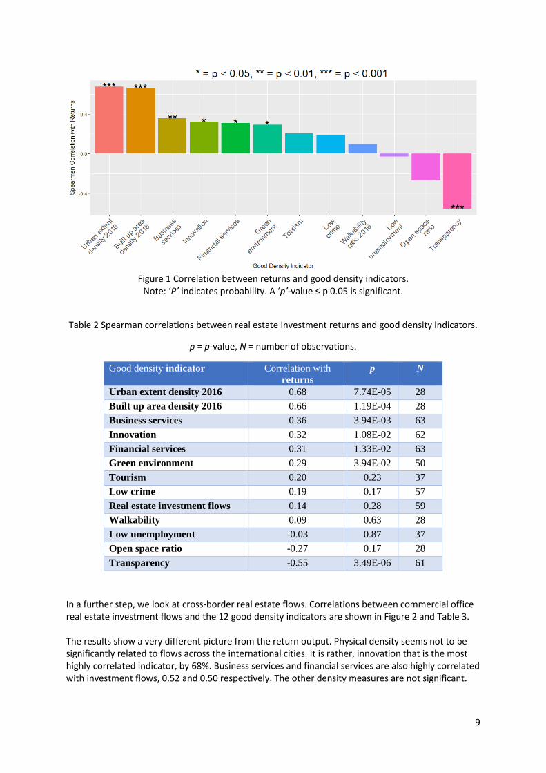
Figure 1 Correlation between returns and good density indicators.
Note: ‘P’ indicates probability. A ‘p’-value ≤ p 0.05 is significant.
Table 2 Spearman correlations between real estate investment returns and good density indicators.
p = p-value, N = number of observations.
Good density indicator Correlation with
returns
p N
Urban extent density 2016 0.68 7.74E-05 28
Built up area density 2016 0.66 1.19E-04 28
Business services 0.36 3.94E-03 63
Innovation 0.32 1.08E-02 62
Financial services 0.31 1.33E-02 63
Green environment 0.29 3.94E-02 50
Tourism 0.20 0.23 37
Low crime 0.19 0.17 57
Real estate investment flows 0.14 0.28 59
Walkability 0.09 0.63 28
Low unemployment -0.03 0.87 37
Open space ratio -0.27 0.17 28
Transparency -0.55 3.49E-06 61
In a further step, we look at cross-border real estate flows. Correlations between commercial office real estate investment flows and the 12 good density indicators are shown in Figure 2 and Table 3. The results show a very different picture from the return output. Physical density seems not to be significantly related to flows across the international cities. It is rather, innovation that is the most highly correlated indicator, by 68%. Business services and financial services are also highly correlated with investment flows, 0.52 and 0.50 respectively. The other density measures are not significant.

10
The results suggest that the innovation and quality of services of a city are what is associated with good density when it comes to real estate flows rather than the more traditional measures of urban form. However, the analysis does not account for omitted variables relevant to commercial office demand and supply drivers of real estate capital flows, such as space demand and supply.
Figure 2 Correlation between real estate investment flows and good density indicators.
Table 3 Spearman correlations between good density indicators and real estate investment flows.
Good density indicator
Correlation with
Real investment
flows
p N
Returns before 2008 0.14 0.28 59
Business services 0.52 1.97E-05 59
Financial services 0.50 5.86E-05 59
Innovation 0.68 2.97E-09 59
Low unemployment 0.18 0.30 37
Low crime -0.05 0.72 54
Green environment 0.16 0.27 48
Transparency -0.07 0.58 58
Urban extent density 2016 -0.10 0.62 27
Built up area density 2016 -0.13 0.53 27
Open space ratio -0.09 0.66 27
Walkability ratio 2016 -0.09 0.67 27
Tourism 0.21 0.23 35

11
European insight Figures 3 to 6 and Tables 4 to 7 show correlations discovered between the 12 good density indicators and real estate capital values and rents for retail as well as office markets for nine European cities where urban form density data were also available: London, Paris, Moscow, Milan, Madrid, Berlin, Vienna, Warsaw and Budapest. Given the small sample size (nine cities), generalization on the basis of these results is not possible, however, they offer interesting insights into relationships presenting in selected European mature and developing office and retail markets. The results overall are in line with the results shown in Figure 1 for the extended sample, confirming that urban extent and built up density measures have the highest correlation with office capital values. Though significance for property performance is not demonstrated, open space ratio is generally negatively correlated with office and retail capital values and rents. Innovation and investment flows are positively correlated with office capital values (by 0.52 and 0.48 respectively – Table 4 and with retail rents (by 0.63 and 0.54 respectively -Table 7). The strong positive correlation of tourism along with business services with retail capital values (0.55 and 0.47 respectively – Table 6), is of potential interest for further research given that tourism is likely to reflect qualitative aspects of city good density for which reliable global data have not been identified for this study. Tourism is also positively correlated (though without significance) with office capital values, by 0.33 (Table 4) and with retail rents, by 0.43 (Table 7). Tourism resurfaces again later as of interest in relation to investment returns in portraits of cities in developed economies (London, Paris and Hong Kong). The general lack of significance of walkability found in both the global and the European results, seems likely to reflect the fact that AoUE walkability is a city level metric and does not account for sub-city density variations associated with commercial land use (see Technical Annex IB). Based on the literature reviewed in Phase I, proximity is an important driver of commercial clustering within cities and walkability follows from this (see Technical Annex IB).
Figure 3 Correlation between office capital values and good density indicators.

12
Figure 4 Correlation between office rents and good density indicators.
Figure 5 Correlation between retail capital values and good density indicators.

13
Figure 6 Correlation between retail rents and good density indicators.
Table 4 Correlation between city office capital values (CVs) and good density indicators. p = p-value, N = number of observations.
Correlation with
office CVs p N
Office rents 0.27 0.22 23
Retail rents 0.22 0.30 24
Retail CVs 0.49 1.45E-02 24
Real investment flows 0.48 2.07E-02 23
Business services 0.09 0.66 24
Financial services 0.06 0.77 24
Innovation 0.52 0.01 24
Green environment -0.02 0.95 21
Transparency 0.29 0.17 24
Urban extent density 0.80 9.63E-03 9
Built up area density 0.73 2.46E-02 9
Open space ratio -0.33 0.38 9
Walkability ratio 0.03 0.93 9
Tourism 0.33 0.20 17
Low unemployment -0.19 0.42 20
Low crime -0.18 0.43 22
14
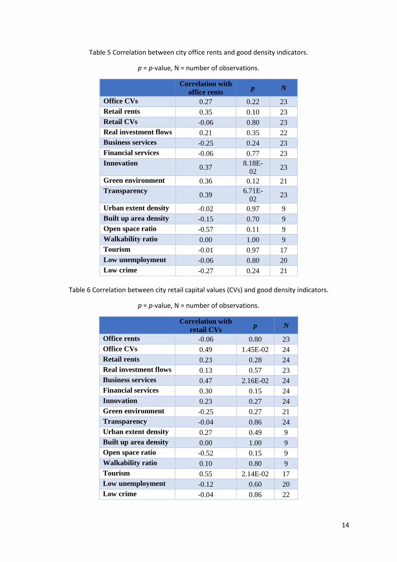
Table 5 Correlation between city office rents and good density indicators.
p = p-value, N = number of observations.
Correlation with
office rents p N
Office CVs 0.27 0.22 23
Retail rents 0.35 0.10 23
Retail CVs -0.06 0.80 23
Real investment flows 0.21 0.35 22
Business services -0.25 0.24 23
Financial services -0.06 0.77 23
Innovation 0.37
8.18E-
02 23
Green environment 0.36 0.12 21
Transparency 0.39
6.71E-
02 23
Urban extent density -0.02 0.97 9
Built up area density -0.15 0.70 9
Open space ratio -0.57 0.11 9
Walkability ratio 0.00 1.00 9
Tourism -0.01 0.97 17
Low unemployment -0.06 0.80 20
Low crime -0.27 0.24 21
Table 6 Correlation between city retail capital values (CVs) and good density indicators.
p = p-value, N = number of observations.
Correlation with
retail CVs p N
Office rents -0.06 0.80 23
Office CVs 0.49 1.45E-02 24
Retail rents 0.23 0.28 24
Real investment flows 0.13 0.57 23
Business services 0.47 2.16E-02 24
Financial services 0.30 0.15 24
Innovation 0.23 0.27 24
Green environment -0.25 0.27 21
Transparency -0.04 0.86 24
Urban extent density 0.27 0.49 9
Built up area density 0.00 1.00 9
Open space ratio -0.52 0.15 9
Walkability ratio 0.10 0.80 9
Tourism 0.55 2.14E-02 17
Low unemployment -0.12 0.60 20
Low crime -0.04 0.86 22
15
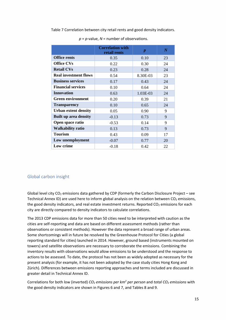
Table 7 Correlation between city retail rents and good density indicators.
p = p-value, N = number of observations.
Correlation with
retail rents p N
Office rents 0.35 0.10 23
Office CVs 0.22 0.30 24
Retail CVs 0.23 0.28 24
Real investment flows 0.54 8.30E-03 23
Business services 0.17 0.43 24
Financial services 0.10 0.64 24
Innovation 0.63 1.03E-03 24
Green environment 0.20 0.39 21
Transparency 0.10 0.65 24
Urban extent density 0.05 0.90 9
Built up area density -0.13 0.73 9
Open space ratio -0.53 0.14 9
Walkability ratio 0.13 0.73 9
Tourism 0.43 0.09 17
Low unemployment -0.07 0.77 20
Low crime -0.18 0.42 22
Global carbon insight Global level city CO2 emissions data gathered by CDP (formerly the Carbon Disclosure Project – see
Technical Annex ID) are used here to inform global analysis on the relation between CO2 emissions,
the good density indicators, and real estate investment returns. Reported CO2 emissions for each
city are directly compared to density indicators to calculate correlations.
The 2013 CDP emissions data for more than 50 cities need to be interpreted with caution as the
cities are self-reporting and data are based on different assessment methods (rather than
observations or consistent methods). However the data represent a broad range of urban areas.
Some shortcomings will in future be resolved by the Greenhouse Protocol for Cities (a global
reporting standard for cities) launched in 2014. However, ground based (instruments mounted on
towers) and satellite observations are necessary to corroborate the emissions. Combining the
inventory results with observations would allow emissions to be understood and the response to
actions to be assessed. To date, the protocol has not been as widely adopted as necessary for the
present analysis (for example, it has not been adopted by the case study cities Hong Kong and
Zürich). Differences between emissions reporting approaches and terms included are discussed in
greater detail in Technical Annex ID.
Correlations for both low (inverted) CO2 emissions per km2 per person and total CO2 emissions with
the good density indicators are shown in Figures 6 and 7, and Tables 8 and 9.
16
The CDP data have insignificant correlations between low per capita (per person) emissions, density
indicators, and returns after 2008. However, it is interesting to compare the correlation between
low per capita emissions and commercial office real estate investment returns (0.25, Table 8) with
the weaker correlation for total emissions (0.16, Table 9).
This result agrees with the Phase I literature review conclusions that population and built density
increases are associated with reductions in per capita emissions and increases in per area emissions
(Christen. 2014; Kennedy et al., 2015), suggesting there are efficiency gains despite an overall
increase in emissions from increased population and human activity.
CDP CO2 emissions data are not available for all cities with returns data (for example, for Beijing and
Mumbai, Figure 11). However, of the cities included in this Global Carbon Insight analysis, Hong
Kong, San Francisco and Singapore have the highest office real estate investment returns relative to
low per capita CO2 emissions (Figure 8). Hong Kong also has the strongest relation between high
office real estate investment returns and urban form density (urban extent and built up area) of
cities having both real estate returns and good density data, globally (see mature economy city
profiles and Figure 10).
Paris has similarly high office real estate investment returns to Singapore but also somewhat higher
per capita CO2 emissions (Figure 8) whereas Moscow, Los Angeles and Houston have low per capita
emissions but much lower real estate investment returns than Hong Kong, San Francisco, Singapore
and Paris (Figure 8).
Both Paris and San Francisco have low total CO2 emissions relative to returns (Figure 9).
Interestingly, green environment is positively correlated with low total CO2 emissions (0.34) but there is no correlation between green environment and low CO2 emissions per km2 per person (-0.06), i.e. when accounting for population density. The correlation between transparency and CO2 emissions per km2 per person when excluding US cities (-0.51) was similar to the analysis including all cities (-0.47) demonstrating that this relationship is not a consequence of US cities alone. Questions of how to interpret these relational global patterns requires attention with the benefit of local information and insights, including on the implications of differing measurement methodologies used.

17
Figure 6 Correlation between low CO2 emissions per km2 per person and good density indicators. Note: ‘Low CO2’ reflects that emissions data have been inverted to represent good density. A positive correlation signifies a reduction in CO2 emissions and thereby good density.
Table 8 Correlation between low CO2 emissions per km2 per person and good density indicators.
Good density indicator
Correlation with
CO2 emissions per
km2 per person
p N
Returns after 2008 0.25 0.17 32
Real estate investment flows 0.33 6.85E-02 31
Business services 0.14 0.43 32
Financial services 0.11 0.56 32
Innovation 0.31 8.78E-02 31
Low unemployment 0.24 0.27 23
Low crime 0.14 0.47 30
Green environment -0.06 0.75 29
Transparency -0.47 7.25E-03 32
Urban extent density 2016 0.36 0.16 17
Built up area density 2016 0.38 0.14 17
Open space ratio -0.20 0.44 17
Walkability ratio 2016 0.44 7.45E-02 17
Tourism 0.41 8.23E-02 19

18
Figure 7 Correlation between total low CO2 emissions and good density indicators.11
Table 9 Correlation between low total CO2 emissions and good density indicators.
Good density indicator
Correlation with
total CO2
emissions
p N
Returns after 2008 0.16 0.39 32
Real estate investment flows -0.28 0.12 31
Business services -0.28 0.12 32
Financial services -0.34 0.06 32
Innovation -0.16 0.38 31
Low unemployment -0.10 0.66 23
Low crime 0.10 0.59 30
Green environment 0.34 7.04E-02 29
Transparency -0.10 0.60 32
Urban extent density 2016 -0.26 0.31 17
Built up area density 2016 -0.29 0.25 17
Open space ratio -0.04 0.89 17
Walkability ratio 2016 -0.41 0.10 17
Tourism -0.45 5.59E-02 19
11 The strong negatively correlation of walkability to low CO2 may point to the difference between the AoUE
sourced walkability ratio and whether or not a city is, in fact, walkable, taking into account qualitative criteria (see Technical Annex).

19
Figure 8 Total CO2 emissions per km² per person and real estate investment returns.
Note: Here CO2 emissions data are not inverted and thereby represent ‘bad’ density.

20
Figure 9 Total CO2 and real estate investment returns. Note: Here CO2 emissions data are not inverted and thereby represent ‘bad’ density.
City profiles – Mature & developing economies Six cities were selected from the global level analysis to provide insights into different combinations of good density indicators that are correlated with investment returns in an international commercial office market perspective. The cities are compared here in two separate vignettes examining the cities’ rank positions (percentiles) for real estate returns, capital flows, the 12 good density indicators and CO2 emissions, first for cities in mature economies and, second, for cities in developing economies:
21
o Mature economies: Hong Kong, London and Paris
o Developing economies: Beijing, Mumbai and Warsaw12
Rank percentiles13 are shown in the vignette portraits to draw out different patterns of association
between variables for groups of cities. To distinguish between good density and bad density features
clearly, the employment, crime and CO2 rank metrics are reversed here to show high
unemployment, high crime and high total and per capita emissions for each city.
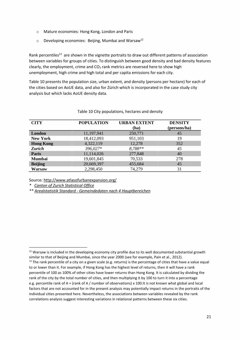
Table 10 presents the population size, urban extent, and density (persons per hectare) for each of
the cities based on AoUE data, and also for Zürich which is incorporated in the case study city
analysis but which lacks AoUE density data.
Table 10 City populations, hectares and density
CITY POPULATION URBAN EXTENT
(ha)
DENSITY
(persons/ha)
London 11,197,941 250,771 45
New York 18,412,093 951,103 19
Hong Kong 4,322,119 12,278 352
Zurich 396,027* 8,788** 45
Paris 11,114,026 277,848 40
Mumbai 19,601,845 70,533 278
Beijing 20,669,397 455,684 45
Warsaw 2,298,450 74,279 31
Source: http://www.atlasofurbanexpansion.org/ * Canton of Zurich Statistical Office ** Arealstatistik Standard - Gemeindedaten nach 4 Hauptbereichen
12 Warsaw is included in the developing economy city profile due to its well documented substantial growth similar to that of Beijing and Mumbai, since the year 2000 (see for example, Pain et al., 2012). 13 The rank percentile of a city on a given scale (e.g. returns) is the percentage of cities that have a value equal
to or lower than it. For example, if Hong Kong has the highest level of returns, then it will have a rank
percentile of 100 as 100% of other cities have lower returns than Hong Kong. It is calculated by dividing the
rank of the city by the total number of cities, and then multiplying it by 100 to turn it into a percentage
e.g. percentile rank of A = (rank of A / number of observations) x 100.It is not known what global and local
factors that are not accounted for in the present analysis may potentially impact returns in the portraits of the
individual cities presented here. Nevertheless, the associations between variables revealed by the rank
correlations analysis suggest interesting variations in relational patterns between these six cities.

22
Hong Kong, London and Paris
Of the cities in mature economies examined, Hong Kong and Paris have the highest office
investment returns (Figure 10). However, Hong Kong’s high urban form density (urban extent and
built up) marks it out from the other cities, not only in the vignette perspective but also in a global
perspective, as already discussed.
Paris notably achieves just slightly lower returns than Hong Kong, with a much lower level of urban
form density. This result indicates that although built form density is generally a major contributor to
higher returns, other aspects of good density, besides urban form, are likely to be important also for
returns in some cities (see Technical Annex IA).
A common pattern amongst the three cities is the strong representation of investment flows,
business services and financial services and, interestingly, tourism. Open space ratio is low for all
three cities.
Other interesting findings from this vignette are, first, Hong Kong’s low open space ratio relative to
urban extent and built up density. Nevertheless it has low crime and unemployment levels relative
to London and Paris.
Second, the relationship between CO2 emissions per person per hectare and total CO2 emissions of
Hong Kong (low emissions per person but high total emissions) is reversed for London and Paris
(lower total than per capita emissions).
Of the three cities, Hong Kong therefore has the highest real estate investment returns (marginally
higher even than Paris) but also the highest total emissions, whereas London has the lowest total
emissions relative to its investment returns despite having lower built up and urban extent density
than Hong Kong.

23
Figure 10 Good density profiles for Hong Kong, Paris and London.
Note: CO2 emissions data are not inverted and therefore represent ‘bad’ density.
Beijing, Mumbai and Warsaw
Of interest in studying the patterns of relationships between good density indicators for the cities in
developing economies, is that although investment flows, business services and financial services are
most highly represented in Beijing, it is Mumbai that has the highest urban form density and also the
highest returns of all three cities (Figure 11). Nevertheless, both Mumbai and Beijing have higher
urban form density than the European cities analyzed in the two vignettes (Paris, London and
Warsaw).
Each of the three cities has a high representation of business services nevertheless and, to varying
degrees, financial services. However, it is striking that innovation, which was shown to be highly
correlated with returns at the global level, is relatively less well represented here, especially for
Mumbai and Warsaw. Also, tourism, which is strongly represented in the mature economy cities, is
far less prominent amongst the good density indicators in these developing economy cities.
Green environment and transparency are also low for all three cities, especially green environment
for Beijing and transparency for Mumbai. Open space ratio is lowest for Mumbai. In the context of
the negative correlation of open space ratio with returns at a global level, the ratio for Beijing stands
out however, demanding further investigation employing local information.

24
Warsaw has the lowest returns of the three cities despite its relatively high business services
representation. The city’s recent rise, along with other Polish cities, as a location for business
processing activities as opposed to the more specialized financial and business services that are
concentrated in mature economy cities may explain this apparent anomaly (Pain and Van Hamme,
2014; Cushman Wakefield, 2016).
Other positive good density indicators represented for Warsaw are a high open space ratio relative
to that of Mumbai, and low crime relative to both cities, especially Mumbai. CO2 emissions data are
not available for Mumbai and Beijing. Warsaw has higher total CO2 emissions than emissions per
person per hectare and is thereby in line with the general relationship noted at a global level.
The different patterns of good density indicator relationships with returns and CO2 emissions
between the developing and mature economy cities warrant further examination in discussion with
real estate actors, investment agents, and government bodies in each city. For example, the
potential for tourism and innovation in future to act as contributing significant factors supporting
returns and capital flows alongside existing urban form density and business and financial services.
The results on CO2 emissions, total and per capita, and their relationships with open space and green
environment and returns for cities in mature and developing economies requires in-depth local
investigation into confounding variables such as patterns of travel by car linked to urban form and
differences in climate, rainfall, vegetation and growing seasons that impact emissions in cities in
different world locations.
Figure 11 Good density profiles for Beijing, Mumbai and Warsaw.
Note: CO2 emissions data are not inverted and therefore represent ‘bad’ density.
25
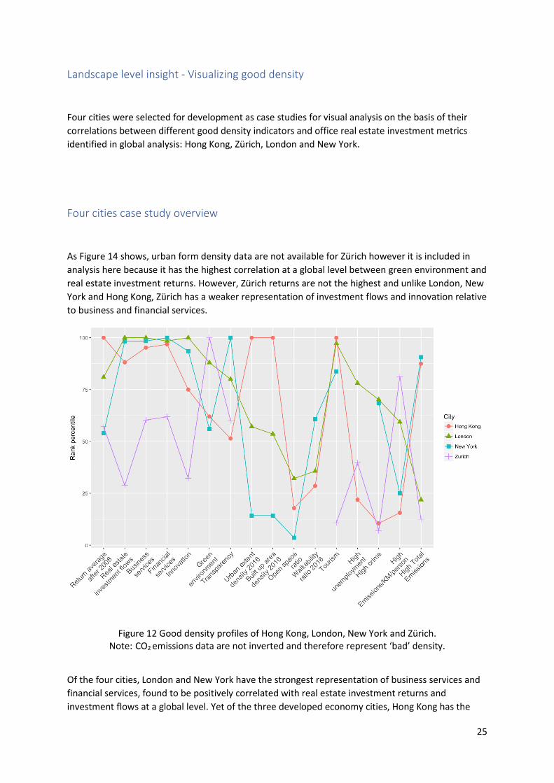
Landscape level insight - Visualizing good density
Four cities were selected for development as case studies for visual analysis on the basis of their
correlations between different good density indicators and office real estate investment metrics
identified in global analysis: Hong Kong, Zürich, London and New York.
Four cities case study overview
As Figure 14 shows, urban form density data are not available for Zürich however it is included in
analysis here because it has the highest correlation at a global level between green environment and
real estate investment returns. However, Zürich returns are not the highest and unlike London, New
York and Hong Kong, Zürich has a weaker representation of investment flows and innovation relative
to business and financial services.
Figure 12 Good density profiles of Hong Kong, London, New York and Zürich. Note: CO2 emissions data are not inverted and therefore represent ‘bad’ density.
Of the four cities, London and New York have the strongest representation of business services and
financial services, found to be positively correlated with real estate investment returns and
investment flows at a global level. Yet of the three developed economy cities, Hong Kong has the

26
highest returns. This pattern of association supports the general finding on the significance of
compact built density for investment returns. The strong relationship between urban extent density
and built up density and returns for Hong Kong contrasts with the lower urban form density of
London, and especially New York.
Despite New York having lower investment returns than Hong Kong and London (and the lowest
urban form density of all four cities), in common with Hong Kong, it has a low open space ratio along
with high total CO2 emissions and low per capita emissions. It is interesting to speculate whether
Zürich’s high green environment score is related to its low level of total CO2 emissions.
Visual analysis for good density
London was found to have the most accessible sources for city and sub-city level data required for
visual analysis and was therefore able to be developed to include a series of metric overlays
illustrated in example Exhibits 1-4. The London visual mapping tool, demonstrates the potential
value of visual analysis for informing private and public sector investment on the spatial structure of
good density and the relationships between urban form characteristics at a landscape level. Exhibit 1
shows air quality, transport and property deals on one screen to illustrate how individual maps can
be overlaid to assist spatial analysis and inform decision making.
Exhibit 1 London air quality, transport and top-20 property deals, 2014 (first three quarters).
Future in-depth research would allow the incorporation of more detailed local micro- and property
level data for other cities and across larger functional urban area scales that spill over official

27
metropolitan boundaries (Hall and Pain, 2006) and which will have different local residential and
employment market structures that are determinants of mobility patterns, CO2 emissions and
displacement (see Technical Annex ID).
Findings from the Phase I literature review suggest that urban form and open space patterns within
cities are significant influences on the location and the magnitude of CO2 emissions. Therefore,
visual mapping assisted management of open space ratios in densely developed areas, has potential
value in terms of reducing emissions and in supporting resilient property values and returns.
Real estate investment
Real Capital Analytics property transactions data have been incorporated in visualization for the top-
10 office deals in the period 2007-14 in each of the four cities to illustrate the spatial pattern of
major investment flows and concentration in their respective office property markets.
For London, the top-20 transactions in 2014 (1st three quarters) are shown in Exhibit 2, confirming
the localised clustering and concentration of high-value transactions found common in each city.
This spatial pattern highlights the significance of land values, building heights and commercial floor
space, for major investment flows, that are not apparent from the population based density metrics
incorporated elsewhere in analysis.
The lower top-ten transactions value for Zürich (6%) will reflect its smaller global business and
financial services and commercial office market size relative to New York (40%), London (35%), and
Hong Kong (18%).
Exhibit 2 London top-20 property deals, 2014 (first three quarters).

28
Carbon emissions
For CO2 emissions/km2/person 2015, the rank order of the four case study cities from lowest to
highest emissions km2/per person is: Hong Kong (rank 1), New York (rank 2), London (rank 3), Zürich
(rank 4) however, the data for Zürich can’t be directly compared with that for the other three cities
due to the use of different definitions used in city analysis (see Technical Annex ID). Furthermore,
city-level statistics can obscure important variations at finer-scales.
Visualization techniques can reveal heterogeneity that is important to frame investment and policy.
Exhibit 3 illustrates the incorporation of borough level data illustrating CO2 emissions variations in
London and the location of high CO2 levels in the central business district and around the Heathrow
air and the motorway complex to the west of the city.
Findings from the Phase I literature review suggest that increasing urban density can act to displace
emissions to less dense, less regulated areas. For example, people may decide to live outside an
urban greenbelt and commute into the city from a suburban community. In this situation, a portion
of transportation emissions have been displaced outside of urban boundaries, but the total
emissions may not have been reduced. Within a city, the distribution of open space will also affect
spatial patterns of urban density as well as CO2 emissions.
Urban CO2 emissions are a result of complex scale interactions between urban form, including open
green and blue space, climate, environmental and social, economic and market factors. Therefore, a
simple correlation between total CO2 emissions and real estate investment does not take into
account local differences in climate and emissions from building heating for example.
Different growing seasons between cities, for example, in high latitudes vs low latitudes, vegetation
amounts (e.g. the inner city in London vs residential London have very different amounts of
vegetation) which will offset some CO2 emissions whereas seasonal bare vegetation will also emit
CO2 , and this will change with climate.
The complex interrelations between determinants of both total and per capita emissions illustrates
the need for global studies to be informed by more comprehensive and accurate local data and the
development of relevant metrics such as CO2 per unit floor space or relations between per capita
emissions and per capita GDP with which to compare diverse cities. This work was beyond the scope
of the present research.

29
Exhibit 3 London energy and greenhouse inventory, 2012.
Public transportation infrastructure & costs
Exhibit 4 incorporates the London example of the public Underground transport network in
visualization. The location of stations shown here is of particular importance for accessibility.
Mapping inter-modal transport hubs is also important in relation to passenger and freight transport
mode exchanges, for example, from cars to mainline rail services (Hall and Pain, 2006). Investment in
public transportation infrastructure and services provision could help to reduce CO2 emissions and
displacement of those emissions which impact in dense city locations (Foster et al., 2010).

30
Exhibit 4 London public underground and stations.
Figures 13 to 15 provide information on public transport data, including costs and passenger
numbers, for each of the four case study cities.
In theory, public transport unit operating and routine maintenance/renewal costs should fall with
greater density, all things being equal, due to fuel efficiencies, shorter routes, etc. however other
key factors play a part in the determination of actual costs, such as physical aspects
(topography/geography of a city), different funding/organisational models and type of local
economy/employment (determining travel needs).
Public transport costs per passenger are greater in London and New York than in Hong Kong. Density
of population and spatial variations in housing costs (and therefore average length of journey) may
play a part however this may be due in large part to differences in labour and other unit costs. Due
to issues of differing cost definitions, caution is needed in comparing estimates of operating costs
per passenger between the cities however they are consistent with London Transport Authority
study findings (LTA, 2011, p. 5, - see Technical Annex IE).
The link between public transport infrastructure costs and good density and by extension
investment returns is complex and deserving of much further research beyond this project. In theory
there is a likely link between transport operating costs (indicating size and usage of a city public
transport network) and CO2 emissions, and more generally with business efficiency in terms of
worker and client accessibility, and their costs of transport options. Likely specific good density
indicator relationships are: employment, business services, green environment, tourism, and
walkability (due to lower car usage) although others such as crime would be interesting to look at
too in a larger follow up study.
The literature reviewed highlights the great importance of public transport infrastructure
investment for both sustainable development and sustained economic growth (for example, Taylor
et al., 2003; Hall and Pain, 2006). Bearing in mind the data limitations encountered (see Technical

31
Annex), the relationship between transportation infrastructure costs, good density and sustained
real investment flows and performance therefore warrants joined-up public-private sector decision-
making attention. Securing comparability of data between cities is a relevant part of the research
and decision-making processes in order that comparable datasets can be used to analyse the link to
good density.
Figure 13 Public transport passengers and shares of transport market14 in 2015/16.
14 Share of transport market refers to the percentage of passenger journeys by public transport compared to all passenger journeys as reported through travel surveys.
0 20 40 60 80 100
0 500 1000 1500 2000 2500 3000
London
Zurich
Hong Kong
New York
%
Million
Passengers in 2015/16
Share of Transport Market

32
Figure 14 Public transportation total operating expenditure and per passenger2015/1615
Figure 15 Public transportation total capital expenditure and per passenger 2015/16
15 Caution is needed in comparing city operating costs. In particular, the New York operating cost total is likely to include renewal and maintenance expenditures (for which no separate figures were found) while these expenditures are not included in the other city operating cost totals.
0 1 2 3 4 5 6
0 5000 10000 15000 20000
London
Zurich
Hong Kong
New York
USD
Million USD
Operating Expenditure2015/16 (Mill USD)
Operating Expenditure perpassenger 2015/16 (USD)
0 0.2 0.4 0.6 0.8 1 1.2
0 1000 2000 3000 4000
London
Zurich
Hong Kong
USD
Million USD
Capital Expenditure 2015/16(Mill USD)
Capital Expenditure perpassenger (USD)

33
Successful investing in density - implications for investment and policy
decision-making
This study set out to evaluate the impact of investment in compact, connected urban development
on returns for real estate investors and the implications for CO2 emissions and infrastructure cost
per resident for the public sector. Here we reflect upon the results overall to identify concluding
inferences. Despite data availability limitations encountered preventing advanced econometric
analysis, the Spearman approach to analysis has revealed interesting contemporary patterns of
association (Spearman, 1904) between real estate, good density variables and CO2 emissions which
have implications for infrastructure investment for city governments.
Good density and real estate investment performance
While the direction of causality between real estate returns and good density variables is not clear,
the research shows where there are strong positive relationships which can inform decision making
on appropriate density measures relative to investment data. Positive and negative correlations
identified have been validated using significance tests (see Technical Annex IC and IF).
For the largest sample of cities analyzed, nine variables have been found to be positive measures of
good density for purposes of real estate investment in commercial office assets. Six of these are
significant, however tourism is shown to be strongly associated with returns in some cities.
GOOD DENSITY GRADIENT – OFFICES (Returns)
Urban extent density ***
Built-up area density ***
Business services **
Innovation *
Financial services *
Green environment *
Tourism
Low crime
Walkability
Note: Significance: * = p < 0.05; ** = p < 0.01; *** = p < 0.001.
34
Urban extent and built up area density are the most strongly positively correlated variables with
office returns, providing quantitative evidence that more densely developed cities are associated
with higher returns for investors. The association between real estate performance and dense,
compact urban development is confirmed by the results on office capital values for nine major
European cities (London, Paris, Moscow, Milan, Madrid, Berlin, Vienna, Warsaw and Budapest). This
is an important result given the dearth of real estate studies directly investigating the spatial
determinants of investment performance empirically.
Relevant for policy makers, the results also demonstrate that population and built densities highly
related to returns, are associated with reductions in per capita CO2 emissions. In other words,
despite the overall increase in emissions associated with increased population size and human
activity, dense cities have efficiency gains.
Investment in dense cities can therefore be expected in general to have notable ‘win-win’
advantages in terms of returns on investment and mitigation of climate change in the context of
contemporary continued world population increase and urbanization (United Nations, 2017).
Some general differences between patterns of association between good density and returns are
found in mature and developing markets. In addition, variations exist for individual cities within
these markets, as illustrated for example by mature economy cities Hong Kong vs Paris, and
developing economy cities Warsaw vs Mumbai.
In addition, city level analyses show that even though statistical significance of correlations with
returns is not demonstrated at the global level for all nine positively correlated variables, tourism is
nonetheless strongly represented in the four mature economy city cases, Hong Kong, London, Paris
and New York. So the balance between positively and negatively related density variables to returns
in each case examined, sheds light on important issues for city investment, risk-adjusted returns and
priorities for policy in different world locations.
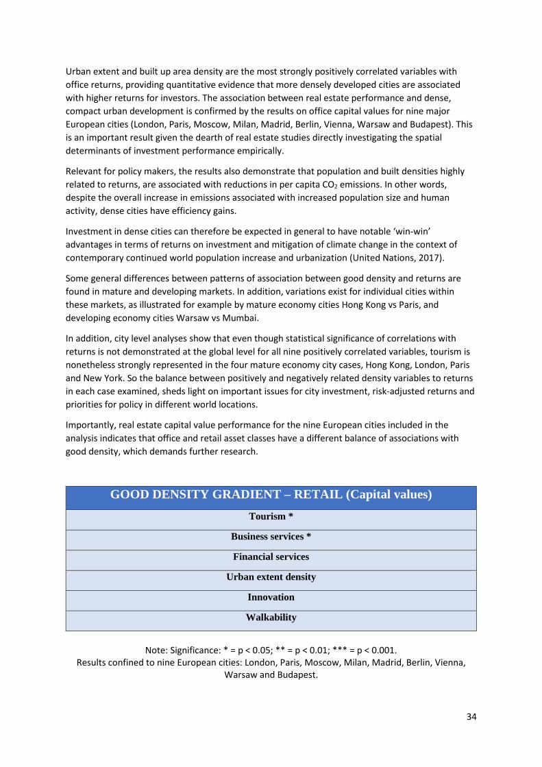
Importantly, real estate capital value performance for the nine European cities included in the
analysis indicates that office and retail asset classes have a different balance of associations with
good density, which demands further research.
GOOD DENSITY GRADIENT – RETAIL (Capital values)
Tourism *
Business services *
Financial services
Urban extent density
Innovation
Walkability
Note: Significance: * = p < 0.05; ** = p < 0.01; *** = p < 0.001.
Results confined to nine European cities: London, Paris, Moscow, Milan, Madrid, Berlin, Vienna, Warsaw and Budapest.
35
Furthermore, contemporary dynamic changes in the retail sector including the location of property
assets and linked goods supply chain logistics and consumer travel patterns (Dawson, 2012) can be
expected to have a bearing on carbon emissions across cities and wider urban regions.
The significance of tourism and business services for retail performance in the European context is of
interest given the association of both variables with high office returns in a global perspective in the
mature economy city portraits.
The other good density indicators for which data were available for comparative analysis have not
been found to be positively correlated with real estate performance. However, the results highlight
that a focus on individual cities is necessary to deepen understanding of nuances important in
understanding relationships between both good and bad density, and property performance.
Implications for risk-adjusted real estate returns
The research indicates that investor judgements regarding whether returns can be expected to be
positively or negatively correlated for specific commercial office and retail investments, and
associated risk, should take city good and bad density into account alongside other sources of risk
applied in standard property level comparative risk indices (i.e. debt, leasing, building, tenant, etc.).
The calculation of risk-adjusted returns commonly assumes that increased risk exposure (for
example, associated with opportunistic investments) should, in theory, attract an increased return
on investment. However, a key message from this research is that bad density in the form of open
space ratio is negatively correlated with returns across asset classes and performance measures.
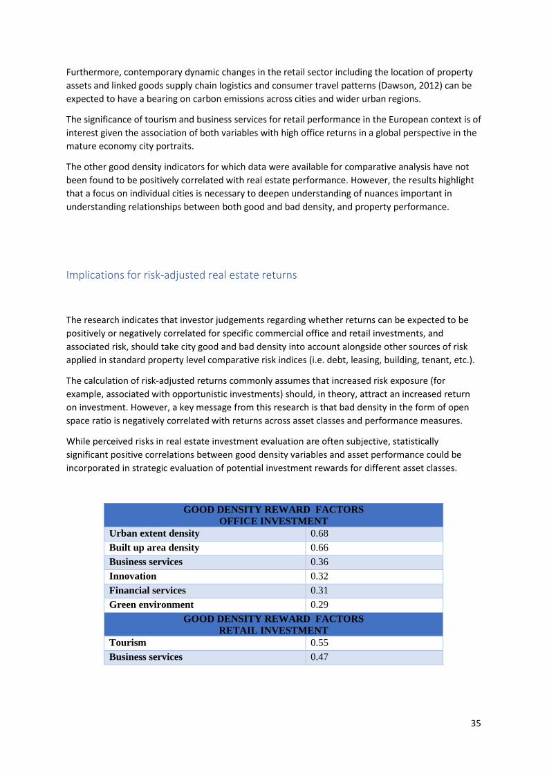
While perceived risks in real estate investment evaluation are often subjective, statistically
significant positive correlations between good density variables and asset performance could be
incorporated in strategic evaluation of potential investment rewards for different asset classes.
GOOD DENSITY REWARD FACTORS
OFFICE INVESTMENT
Urban extent density 0.68
Built up area density 0.66
Business services 0.36
Innovation 0.32
Financial services 0.31
Green environment 0.29
GOOD DENSITY REWARD FACTORS
RETAIL INVESTMENT
Tourism 0.55
Business services 0.47

36
Bearing in mind the data limitations emphasized in this report, this research suggests that in
calculating comparative risks and rewards for competing investment opportunities in commercial
office markets, property in high density cities with strong business services, innovation, financial
services and green environment, should have a higher return score and a lower risk score than
equivalent property in cities performing less well on these measures. Similarly, in calculating
comparative risks and rewards for competing investment opportunities in retail markets, property in
cities with strong tourism and business services, should have a higher return score and a lower risk
score than equivalent property in cities performing less well on these measures. By assigning
quantitatively researched good and bad density scores to investment evaluation, calculation of the
balance between overall risks and rewards of competing opportunities could be better informed.
In addition to the need to take into account different relations between good density and office vs
retail asset classes, the research shows that investors should take a market (developed vs emerging)
and city-specific decision-making approach to investment in order to achieve more accurate
assessment of potential rewards and risk at the property level; for example, despite its negative
correlation with performance in general, open space ratio varies for different cities.
Of the cities in the world with complete data available for office returns and good density variables,
the profiles of thirteen cities manifesting interesting associations for eight variables, including
tourism, are illustrated next using simple traffic lights colour coding to denote differences in overall
patterns based on percentile rankings: Red – low (0-25); Amber – median (25-75); Green – high (75-
100). The cities are split into two groups according to their existing returns performance to illustrate
aspects of good density that may need to be improved in order to either boost or sustain their
returns performance going forward.
Incorporation of local good and bad density data based on visual analysis would allow the
incorporation of property-level risk associated with density, for example, asset location relative to
public transport nodes and green space vs traffic flows, congestion, displaced CO2 .and air quality.
Both city and property-level density data (illustrated in the visualization tool demonstrator) need to
be considered in order to achieve optimal risk-adjusted returns for short-term holding periods and,
at the same time, to invest in and assure good density that is essential for long-run sustainable
development and portfolio resilience. The case of New York in particular (Figure 12), illustrates the
need for sub-city analysis to accurately pinpoint good density within large urban areas.
Analyses incorporating time series data would allow good and bad density trajectories of individual
cities to be taken into account in policy and investment decision making. This is particularly relevant
for emerging economies where rapid urbanization and increasing concentration of business and
financial services are occurring. For example, this research found that Guangzhou in China ranked
17th city in the world for financial services concentration and had returns on commercial office real
estate investment that exceeded those for New York.

37
SAFE HAVEN CITIES?
Hong Kong
Mumbai
Paris
Singapore
Taipei
Shanghai
London
Madrid
Beijing
CITIES OF OPPORTUNITY?
Seoul
Istanbul
New York
Sydney
Return
Urban extent density
Built up
density
Business Services
Innovation
Financial Services
Green
Environment
Open space
Tourism
Note: The CBRE returns data do not include Japanese cities – see Annex IC.

38
Supporting smart urban growth – agenda for real estate, policy and
research
When the quantitative results are reflected upon against the backdrop of the literature reviewed,
patterns of association revealed by the Phase II quantitative correlations and rank percentile city
portrait analyses, allow us to highlight eight specific issues for good density requiring the particular
attention of decision makers and further research: ‘urban density’, ‘tourism’, ‘CO2 emissions’,
‘walkability’, ‘open space’, ‘green environment’, ‘transport’ and ‘urban form’.
Urban density
The major observation from global analysis that dense urban form (urban extent and built-up area)
goes along with strong office real estate investment performance, is best illustrated by Hong Kong
which has the highest commercial office investment returns and the highest urban form density of
the cities surveyed.
This relationship exists for cities examined in both mature and developing economies, however, the
association between other significant variables (innovation, business and financial services, and
green environment) for returns, varies between markets. For example, Mumbai’s high office returns
are strongly associated with high urban form density while business and financial services and
capital investment flows into the office market are strongly associated with returns in Beijing.
Similarly, the high office returns of Hong Kong are less associated with innovation than is the case
for New York and London. It is noteworthy that London, and especially New York, have lower urban
form density and lower returns than Hong Kong.
Tourism
Although tourism is not found significant for office investment returns or capital flows at the global
level of analysis, in the retail markets of the nine European cities analyzed, tourism is shown to be
highly associated with capital values. Furthermore, the individual developed economy city portraits
suggest that tourism may be associated with high office returns for some cities, as illustrated by
Paris where, despite having a much lower level of urban form density than Hong Kong, only slightly
lower returns are achieved.
The city portraits and the comparisons between them, therefore suggest that although urban form
density is most strongly correlated with returns from a global perspective, other aspects of good
density may also contribute importantly to returns in individual cases. It would seem then that for
some cities, property performance is determined by more than city morphological (population and
physical) density. However, tourism (along with innovation) is less well represented in the
developing economy cities examined, Beijing, Mumbai and Warsaw, and this finding demands
attention in follow-on qualitative research involving local experts.
There is currently a lack of reliable ‘soft’ good density metrics for incorporation in a robust global
comparative quantitative analysis. However, tourism is likely to reflect a number of city qualitative
good density attributes that together have significance for property performance measures. The

39
results on tourism for retail performance as well as for office performance for mature economy
cities, provides quantitative evidence supporting the hypothesis of the commutability of cultural
capital to economic capital in cities (Pain, 2008a).
Carbon emissions
Albeit significance is not demonstrated, combining all good density and office performance variables
in global CO2 analysis shows a positive correlation between nine urban form density indicators,
urban low per capita CO2 emissions and returns on investment (0.25). By contrast, ten good density
variables are negatively correlated with low total CO2 emissions (returns correlation, 0.16).
Recent United Nations statistics indicate that the present global population of nearly 7.6 billion has increased by one billion people in just over one decade (United Nations, 2017). The efficiency gains found for dense/compact cities in terms of reductions in per capita emissions despite their population size, intense activity and mobility, is therefore clearly of great importance in the context of world population growth. For the mature economy cities included in the portraits, it is noteworthy that, similar to Hong Kong,
Paris has very high returns but it achieves this returns level with lower built up and urban extent
density coupled with higher per capita CO2 emissions than total emissions. This relational pattern
implies that there may be scope to deliver higher carbon efficiency gains in Paris with a higher
density urban form development scenario going forward. However densification would need to be
sensitive to impacts on other good density characteristics in a spatial context, for example, tourism,
open and green space.
Comparable emissions data for Beijing and Mumbai were unavailable for the present study, however, the United Nations (2017), highlights that China and India remain the two most highly populated countries in the world, with 19 and 18 per cent of the global population total respectively (United Nations, 2017). The findings on the correlation between morphological density, economic and financial services and investment performance for Mumbai and Beijing demonstrate the case for built form density in these rapidly developing and urbanizing economies. CO2 displacement and local concentrations highlight risks for human health and well-being
associated with other traffic associated air pollutants, illustrated by the visualization tool for London.
Therefore, the negative correlation of low CO2 emissions per km2 per person with urban extent and
built up area density, requires further investigation.
Walkability
The research results demonstrate that the relevance of walkability for commercial office and retail
property performance cannot be demonstrated based on satellite data alone. Nevertheless, the
correlation between innovation, business and financial services and property performance is
indicative of a relationship with walkability.
Literature reviewed in Phase I of the study indicates that innovation in these knowledge-intensive
economic sectors is dependent on clustering and close proximity (Taylor et al., 2003), walkability is
therefore implied. Furthermore, there is evidence from a small emerging real estate literature of
links between spatial proximity and property returns (for example, Zhu and Milcheva, 2016).

40
However, as discussed in Technical Annex IB, physical proximity does not necessarily mean that a
place or route is environmentally pleasant or safe to walk.
Given the results from this study on total CO2 emissions, their spatial displacement, and the
implications of intense traffic flows and congestion for air quality and human health (for example,
nitrous oxide exposure, DEFRA/DoT, 2017), an important conclusion is that the environmental
quality of walkable urban spaces should be prioritized in future research, in policy initiatives and in
investment decision making.
Open space
As in the case of tourism, emissions and walkability good density indicators, the correlations for
open space do not show statistical significance for either office or retail property performance.
Nevertheless, it is striking that open space ratio is generally negatively correlated with office returns
and office and retail capital values and rents.
Furthermore, open space ratio is low relative to economic and investment returns for all cities
presented in the city portraits and case studies (Hong Kong, Paris, London, New York, Mumbai) apart
from Beijing and Warsaw (Zürich lacked open space ratio data).
Given the significance of urban form density for investment returns, the contrast between Hong
Kong’s high density and its low open space ratio, illustrates an evident spatial tension underlying the
relationship between city morphological density, returns and open space. This tension seems likely
to impact on housing prices and affordability also.
Green environment
Green environment is one of the good density metrics shown to be positively correlated with office
returns and rents, and (though not significantly) with office capital flows, retail rents and total CO2
emissions.
The individual city portraits reveal city level differences that illustrate interesting patterns across the
mature and developing economy vignettes. Green environment is low relative to economic and
investment measures for Beijing and Mumbai and, to an extent, Warsaw. In contrast, green
environment is higher relative to those same measures for New York, Paris, London and Hong Kong
(this is despite Hong Kong’s low open space ratio) and is highest for Zürich.
From these results it would seem that, as for CO2 and walkability, green environment and its
relationship with open space ratio, demands attention in investment and policy decision making in
order to assure that beyond urban form density, economically successful cities have good density ‘in
the round’. For example, could lessons for good density be learned from Zürich’s high green
environment score relative to its low total CO2 emissions? Urban form density data including on
open space ratio, and local data on car and public transport use for example, would be required to
investigate this pattern of association in depth. Even though no correlation between green
environment and low CO2 emissions per km2 per person was found, in the research literature, green
environment has been found to offset some CO2 emissions.

41
Transport
City infrastructure costs were found to lack consistent recording and reporting, preventing the
incorporation of monetary data in global or European comparative analysis for this study. This
finding highlights an important area for national government attention internationally in view of the
relevance of public-private sector financing for infrastructure in general.
Transportation infrastructure is highlighted by the present research as being of critical importance
for good density. Not only is public transportation infrastructure a fundamental requirement to
support accessibility and connectivity for economically sustainable cities and linked property
investment but this research demonstrates its critical importance for reducing emissions linked to
climate change and supporting the sustainability of green environment, air quality and human
health, locally.
As highlighted by literature reviewed in Phase I, both physical public transportation infrastructure
and efficient services and capacity must be present in a city. The present study highlights the need
for fine-grained mapping of urban functions and physical clustering at sub city and urban region
scales in order to plan effectively for travel demand and thereby reduce overall CO2 and other
emissions and displacement linked to heavy traffic flows.
Although it has not been possible to incorporate residential assets in the present quantitative
analysis, the literature highlights the impact of locational patterns in housing markets and
affordability, relative to employment and retail development, for the costs and feasibility of public
transportation infrastructure and services provision required to reduce traffic flows by road (Taylor
et al., 2003; Hall and Pain, 2006).
Urban form
The global findings endorse the importance of the six urban form characteristics identified from the
Phase I review of the multi-disciplinary literature as relevant for relationships between good density
and resilient real estate investment returns. The six characteristics underpin successful investment in
density:
Clustering structure and Built infrastructure determine compact development, proximity and
connectivity, open space ratio essential for good density and a green urban environment that
mitigates climate change. Compact urban form (built and urban extent density) and green
environment are found to be positively associated with real estate investment performance.
Economic and Employment structure determines city concentration of high-value economic sectors,
globally networked firms, skilled people and innovation capacity important for a sustainable
economy. Knowledge intensive business and financial services, and innovation, are found to
contribute positively to real estate investment performance.
Public Transport and Green/Blue infrastructures determine the connectedness of cities and
accessibility by modes that limit CO2 emissions and displacement on the one hand and can mitigate
against air pollution and human health risk on the other hand. Green environment is positively
associated with real estate investment performance and public transport can support this.
42
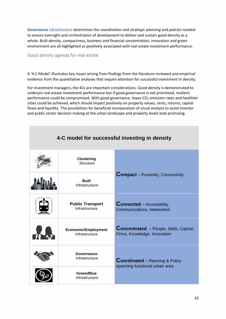
Governance infrastructure determines the coordination and strategic planning and policies needed
to ensure oversight and orchestration of development to deliver and sustain good density as a
whole. Built density, compactness, business and financial concentration, innovation and green
environment are all highlighted as positively associated with real estate investment performance.
Good density agenda for real estate
A ‘4-C Model’ illustrates key issues arising from findings from the literature reviewed and empirical
evidence from the quantitative analyses that require attention for successful investment in density.
For investment managers, the 4Cs are important considerations. Good density is demonstrated to underpin real estate investment performance but if good governance is not prioritized, resilient performance could be compromised. With good governance, lower CO2 emission rates and healthier cities could be achieved, which should impact positively on property values, rents, returns, capital flows and liquidity. The possibilities for beneficial incorporation of visual analysis to assist investor and public sector decision making at the urban landscape and property levels look promising.
4-C model for successful investing in density
Clustering Structure
Compact – Proximity, Connectivity
Built Infrastructure
Public Transport Infrastructure
Connected – Accessibility,
Communications, Networked
Economic/Employment Infrastructure
Concentrated – People, Skills, Capital,
Firms, Knowledge, Innovation
Governance Infrastructure
Coordinated – Planning & Policy
spanning functional urban area
Green/Blue
Infrastructure

43
Good density agenda for planning & policy
Based on the overall findings of Phases I and II of the research, four dimensions of good governance
are singled out for attention to address potential collisions between drivers of good and bad density
acting across different urban functional and spatial scales, and to encourage good density
characteristics required for overall urban resilience as a city’s built up area and urban extent
increase.
Each dimension follows from the key findings from the report and is therefore important to inform
the ‘4-C’ model for successful investment in density. Real estate investment due diligence needs to
take into account the amount of risk likely for a given property investment held for a given time
period. Therefore prospective investments in cities lacking a coordinated governance infrastructure
to support good density should have a higher risk score than for cities with appropriate governance
processes and measures in place.
At the city scale, coordinated action is needed to design into urban form, quality, safe, built and
green environments and open spaces, walkability, transport links, etc. and to protect heritage and
natural green and blue environments (historic buildings, parks, allotments, gardens, vegetation,
rivers, lakes, etc.) which are essential components of good density.
Effective governance incorporating robust data across key metrics from the property scale to the
urban region scale is also needed to plan functional interactions that impact on dense urban spaces
in an integrated way (Hall and Pain, 2006; Barlow et al., 2017).
In the UK, a recent Royal Town Planning Institute response on the UK Government’s 2017 draft UK
Air Quality Plan consultation (DEFRA/DoT, 2017), endorses these key research messages in stressing
the need for Government recognition of the: “critical relationship between urban form,
infrastructure and air quality”, the need “to join up land use and transport planning so that new
developments prioritize active travel – walking and cycling – and public transport”, “to develop
technical capacity to create maps that integrate land, transport and infrastructure” and “to guide
developments towards locations that make use of public transport, walking and cycling” (RTPI,
2017).
Spatial dimension
– Urban form and clustering, land use, mobility patterns
Functional dimension
– Economy, skills and employment, innovation, financial flows
Social dimension
– Accessibility, affordability, appropriate, inclusive
Environmental dimension
– Carbon emissions, air quality, climate change, human and planetary health
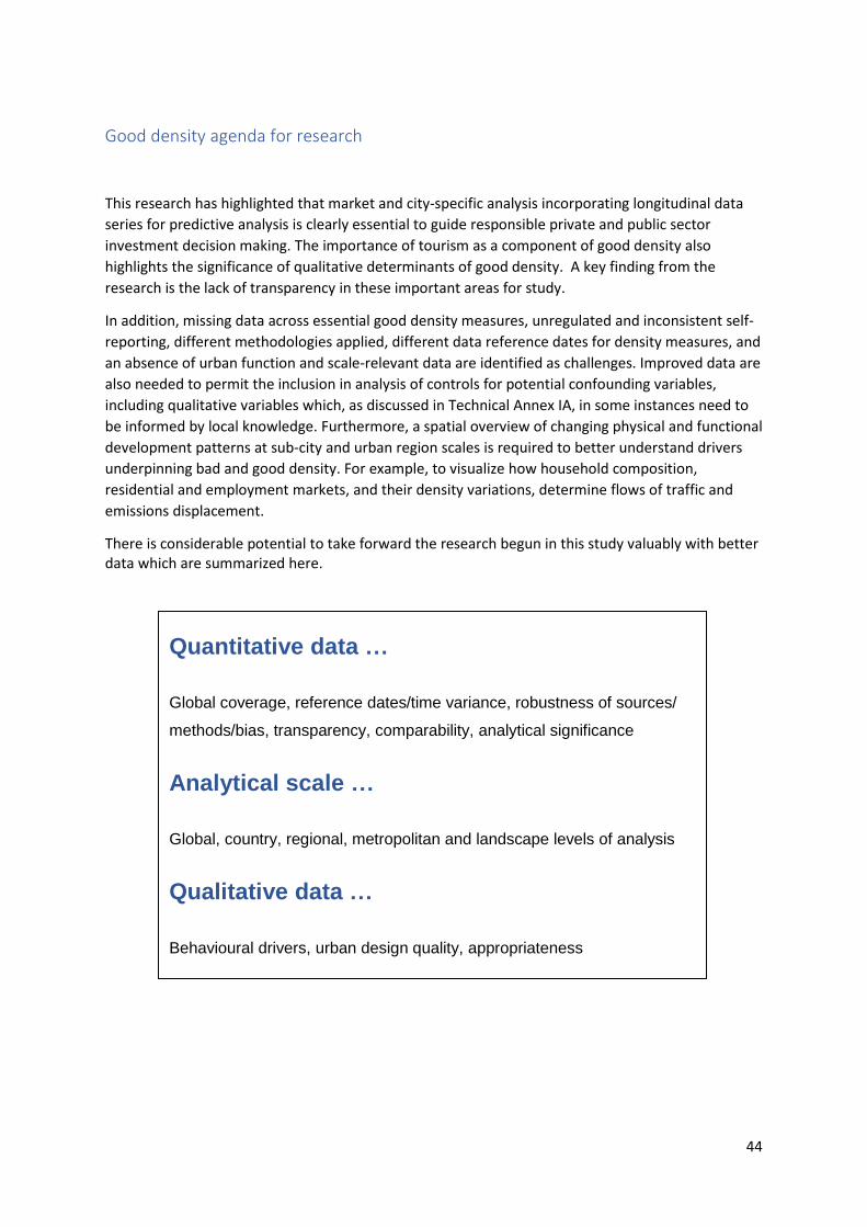
44
Good density agenda for research
This research has highlighted that market and city-specific analysis incorporating longitudinal data
series for predictive analysis is clearly essential to guide responsible private and public sector
investment decision making. The importance of tourism as a component of good density also
highlights the significance of qualitative determinants of good density. A key finding from the
research is the lack of transparency in these important areas for study.
In addition, missing data across essential good density measures, unregulated and inconsistent self-
reporting, different methodologies applied, different data reference dates for density measures, and
an absence of urban function and scale-relevant data are identified as challenges. Improved data are
also needed to permit the inclusion in analysis of controls for potential confounding variables,
including qualitative variables which, as discussed in Technical Annex IA, in some instances need to
be informed by local knowledge. Furthermore, a spatial overview of changing physical and functional
development patterns at sub-city and urban region scales is required to better understand drivers
underpinning bad and good density. For example, to visualize how household composition,
residential and employment markets, and their density variations, determine flows of traffic and
emissions displacement.
There is considerable potential to take forward the research begun in this study valuably with better data which are summarized here.
Quantitative data …
Global coverage, reference dates/time variance, robustness of sources/
methods/bias, transparency, comparability, analytical significance
Analytical scale …
Global, country, regional, metropolitan and landscape levels of analysis
Qualitative data …
Behavioural drivers, urban design quality, appropriateness

45
Some specific research directions that seem valuable to pursue include:
o More detailed European real estate investment insight analysis.
o US real estate investment insight analysis and comparison with Europe (e.g. by incorporating
NCREIF data available for US markets that are a direct measure of total returns).
o Longitudinal analysis of relations between the main components of returns - yields and
capital values - and good density for exogenous factors.
o Incorporation of data distinguishing between different densities, including non-population
based densities (e.g. incorporating UrbiStat data).
o Analysis of how city level ‘collective good densities’, e.g. tourism, innovation, green
environment etc., can, in combination, contribute positively to investment value, returns
and liquidity.
o Data collection and analysis to include building heights and massing to better define,
measure, and understand urban form density (e.g. incorporating LiDAR light detection
remote sensing data).
o Collection of additional detailed local information on public transport services, inter-modal
transfer and connectivity times, and factors determining transport costs and their
relationship to good density.
o Urban functional area analysis incorporating time series data on urban living and work
patterns that contribute to CO2 emissions and displacement across spatial scales, and the
role of open space and green infrastructure in relation to CO2 emissions and human health
and well-being.
o Development of city visualization to incorporate more and better data relevant for good
density-urban form characteristic relationships, for more cities in mature and developing
economies, including modelling being pioneered by the University of Reading Meteorology
research team to allow a consistent methodology to be used within a city, and local context-
specific qualitative appraisal (e.g. design quality).
o Exploration of good density minimum and maximum tipping points/thresholds (e.g. Phase I
expert advisor suggestion that in Hong Kong a plot ratio > 8 is not desirable and evidence on
minimum densities required to support high quality public transport infrastructure).

46
Supporting smart urban growth: Successful Investing in Density TECHNICAL ANNEXES

47
ANNEX I – DEFINITIONS, DATA, SOURCES, METHODS, CHALLENGES
A. Quantitative analysis of the relationship between good density
and real estate investment performance - Overview
The relationship between real estate performance and density is a generally under-explored
research area. However, recent macro level analysis of international real estate investment shows a
concentration of commercial office property capital flows in the dense business districts of financial
centres in the world’s largest economies (Lizieri and Pain, 2014; Henneberry and Mouzakis, 2014;
Stevenson et al., 2014; McAllister and Nanda, 2014; Fuertz, et. al. 2015). At the same time, micro-
level econometric studies focusing on US cities, indicate that physical distance and other measures
of proximity such as economic and financial distance, are an important influence on real estate
investment returns in housing as well as commercial real estate markets (Zhu and Milcheva, 2016;
Milcheva and Zhu, 2016a). Also, at the micro level, spatial relationships between the underlying
properties of real estate companies are shown to have a significant effect on their performance.
Proximity across the property holdings of real estate companies can predict higher return
correlations across the firms, controlling for size, book-to-market, and momentum characteristics
(Milcheva and Zhu, 2016b; Milcheva and Zhu, 2016c).
Quantification of relationships between investment performance and urban form characteristics
representing good density in a global analysis presents significant challenges relating to the
definition, methodologies, quantification, and measurement of good density however.
Defining good density
Density has historically been seen both as a cause and, in recent times, also as a solution to a range
of urban problems (Pain, 1976; Blowers and Pain, 1999; Davis, 2006; Angotti, 2006; Neuwirth, 2006;
Tonkiss, 2014 cited in McFarlane, 2016; Adams at al., 2015). Defining what makes density good as
opposed to a contributor to urban problems is therefore subject to debate. Density defines what a
city is, but it is a relative concept that can relate to different urban characteristics and urban scales
(Davis, 1965; Rapoport, 1975; Bridge, 2009), complicating analysis.
Density can relate to the mix and layout of buildings and property floor space in different uses, to
both ‘open’ private and public space, to economic and financial activity, and to urban resident and
working population, wildlife, crime, disease, traffic, pollution, heat and water, etc., that move into,
out of and within urban space at different scales (Braun, 2006; Adey, 2010). These densities of cities
are uneven and heterogeneous, as opposed to smooth features of development, reflecting constant
variable flows, connectivities and intensities over space and time (Cook et al., 2007; Castells et al.,
2007; Keil, 2014; McFarlane, 2015). Pinning down what ‘good’ density is, and its links with urban
form and real estate performance, therefore requires insights into relationships between many
variables.

48
The definition of ‘good density’ formulated by Clark and Moir (2015) for the Urban Land Institute
which was the basis for the present study reflects the heterogeneity of urban density. Following a
cross-disciplinary literature review in Phase I of the research, the concept of ‘economic density’
which was not represented in the Clark and Moir (2015) definition, was added to analysis by the
research team. This addition was in recognition of the relevance of economic urban form
characteristics for both urban sustainability and investment returns (Lizieri, 2009; Lizieri and Pain,
2014). Agglomerating economic activities such as knowledge-intensive global business and financial
services are regarded in the literature as contributing importantly also to ‘densities of innovation’
(Glaeser and Saiz, 2003; Mahroum et al., 2010; McFarlane, 2016).
The challenges presented for research are set out in detail in this Technical Annex for each of the
four metrics specified for analysis in the research brief in turn, i.e. urban form characteristics, real
estate investment, CO2 emissions, and infrastructure costs to city governments per person. But
beyond more readily quantifiable good density measures, the relationship between good density
and returns is confounded by the qualitative nature of other characteristics of density that together
determine whether density is actually good.
Methodological issues
Following from the number of variables and potential interactions that underpin good density,
qualitative considerations are needed to inform analysis as explained further in relations to urban
form (Martin and Secor, 2014). To reflect the variegated nature of good density, such considerations
should include the quality of property and landscape design, and of the lifestyles, work, and health
and well-being of different social groups, genders and age groups. Differential mobility and access to
urban resources, including open space, and differential exposure to pollution (Guagliardo, 2004;
Graham and McFarlane, 2015), for example, would need to be included in a thoroughgoing analysis
of how good density relates to real estate investment and returns. Qualitative measures of how
human behaviour impacts good density considerations, investment and returns, is of equal
importance, however behavioural research in this field is generally lacking.
Of particular relevance for research on real estate investment and returns are the ways in which
‘sentiment’ and ‘familiarity’ of economic, financial and real estate actors, shapes good density as
well as investment, impacting pricing, liquidity and returns on investment. Such considerations
require attention in international research to allow appropriate control variables to be incorporated
in global modelling (Henneberry and Mouzakis, 2014; Lizieri and Pain, 2014; Milcheva and Zhu,
2016c; Pain, 2017; Akakandelwa et al., 2017).
For example, Henneberry and Mouzakis (2014), argue that the pricing of office property investments
in non-core UK regions is affected by a ‘familiarity’ heuristic adopted by investors who are clustered
in London and who introduce irrational biases in investment location and pricing, ignoring the
intrinsic investment characteristics of those markets. Variations in inherent characteristics of
regional markets are found not to have significant effects on their yields. Investor behaviour is
therefore concluded to constitute a systematic geographical factor behind significant property
supply variations, reducing investment performance.
‘Soft’ qualitative characteristics of cities and real estate markets can therefore be important
determinants of good vs bad density that are confounding variables in present quantitative analysis.

49
Quantification
A void in robust real estate data capable of informing international analysis is also well-established
(Lizieri and Pain, 2014). Deficiencies include a lack of data based on consistent analytical
methodologies and data cleaning, and a lack of data on emerging real estate markets and non-
commercial property required for global comparisons related to good density (Lizieri, 2009; Pain,
2017).
Data on non-real estate good density characteristics have proved similarly elusive to capture for
global level analysis in this research due to variations across characteristics and cities in definitions,
concepts, and analytical frameworks, methods and reporting processes. In addition, both real estate
and other good density data are generally available at country or city level as opposed to sub-city
and city-region levels (Hall and Pain, 2006; Pain, 2006, 2008b, 2012; Taylor et al., 2008; Keil, 2014)
which are shown from the literature reviewed to be critically important scales for analysis of good
density in this study.
Furthermore, census data on urban population, demography, economy, employment and income
and land use and housing price data, fail to reveal the complexity of fluctuating flows (Pain and Hall,
2008) and intensity ‘rhythms’ (McFarlane, 2015) associated with good and bad density at different
spatial scales. Glaeser and Florida and their co-authors, for example, emphasise that not only is
density critical in driving urban success by “speeding the flow of ideas” (Glaeser and Gottlieb, 2009,
p. 1) but also greater levels of urban density and diversity provide the “eternally conducive
environment for generating the human creativity that underpins innovation, entrepreneurship and
economic growth” (Florida et al., 2017, p. 93).
Despite a prolonged and extensive search for robust global indices representative of good density
urban form characteristics able to inform quantitative analysis, just 12 indices were identified to
take forward in analysis (see Annex 1B).
Measurement
Analysis of causal relations between variables in robust multivariate analysis was not possible in the
present study due to some indices providing city rankings only, a general lack of time series data,
variations in data reference years and variations in the number of cities represented in the indices.
Furthermore, in a global scope analysis, the influence of worldwide local factors is unknown.
However, local factors may influence the relationships between good density and real estate value
significantly because value is not simply a by-product of demand for urban property and space use
value, and location. As a portfolio investment, property stores value as a financial asset, and
influences liquidity, capital flows, rents, and capital values, yields and returns on investments (Lizieri,
2009, pp. 181-182; Lizieri et al., 2012). Attempts to explain rental levels for international financial
centres using a standard regression model find anomalies between cities. The largest anomalies are
Mumbai, Dubai and Dublin where predicted rents are substantially higher than observed rents) and
Shanghai, Johannesburg and New York (where observed rents are sharply lower than estimated
costs (Lizieri et al, 2012, p.281). All six anomalies found are explained by local market and economic
contexts.
The significance of local factors and context as determinants of relationships between property
markets and density is reinforced by a recent United States study of the effects of spatial distance
50
from the Boston central business district in shaping Massachusetts population density distribution
(Epifani and Nicolini, 2017). A Bayesian frailty technique is used to control for heterogeneity,
accounting simultaneously for other factors identified with proxies for natural amenities and ethnic
composition in the period 1930-2010 for 51 municipal areas, using the years 1880 and 90 as external
benchmarks. It was found that the city’s accessibility has not always been the dominant determinant
of population density distribution. The influence of other spatial factors working together is
important, such as changes in urban economic structure, ethnicity and the mortgage market. The
results illustrate the need for long time series data in modelling for covariates that reflect locally
specific factors.
So in addition to the need for robust, directly comparable indices for good density and for different
property sectors, these need to be spatially fine-grained with time series data for densely and less
densely researched cities and real estate markets for corresponding spatial scales and time periods
(Lizieri, 2009, p.300).
Limitations of the present analysis
Present research limitations in terms of longitudinal data availability and quality, including data on
qualitative and behavioural factors, mean that variables that may together be significant for real
estate investment and returns cannot currently be accounted for in global analysis. As discussed, a
wide range of factors is potentially significant to what good density is, to the ways that good and bad
densities flux over space and time, and to how those fluxes map onto different cities globally (Clark
and Moonen, 2005) and onto investment returns. Given the complexity of potential
interrelationships and interdependencies between factors underpinning good density highlighted by
the literature reviewed for this study, results from multivariate analysis are likely to be misleading as
a guide to investment.
Instead this research has adopted a simple approach to analysis which illustrates in a
straightforward way, patterns of association between investment returns and a selection of metrics
representing good density urban form characteristics singly. The ‘P’ value, or calculated probability,
is shown for all correlation results presented.16
In this report we present correlations, i.e. relationships between a dependent (returns) variable and
one independent (good density) variable in turn, derived using a Spearman rank correlations analysis
similar to univariate correlations in regression analysis. A Pearson correlation check was run using
data however to check the validity of the rank correlations in the absence of comparable good
density longitudinal data at the global level, no causal or predictive inferences can be assumed.17
There is a need to test the predictive ability of good density for returns in future studies. Our work
provides the groundwork for multivariate regressions incorporating multiple density variables for
cities for which longitudinal data are available. Since multiple variables are likely to interact in
different ways for each city, local assessment based on time series data will be important to frame
16 A p-value weighs the strength of evidence and is always between 0 and 1. A p-value close to 0.05 is considered marginal.
17
51
investment decision-making. What we can say on the basis of the present study is that, of the cities18
and variables examined, density and compactness are well related to real estate investment returns.
Emerging data and analytical methods
In future work, visual analysis of ‘layers’ of heterogeneous urban form characteristics that make and
unmake urban good density trialed in the research could in future projects be assisted by the
incorporation of Internet, satellite and hand-held mobile digital ‘big’ data illustrating fluctuating
flows and intensities to inform private and public sector investment decision making (Cochrane and
Pain, 2004; Sheller, 2004; Harrison and Pain, 2012; Wilson, 2014; Tang et al., 2016; Pain, 2016;
Barlow et al., 2017):
“…certain urban classes are inherently imprecise due to the difficulty in integrating various
social and environmental inputs into a precise definition. Social components often include
demographic patterns, transportation, building type and density while ecological
components include soils, elevation, hydrology, climate, vegetation and tree cover.” (2016,
p. 212)
Potentially, real-time and longitudinal quantitative and qualitative data for individual cities and city-
regions could eventually be used to map fluid changes in the natural and urban built environments,
including building use, heights, floor space and massing, and the movement of people, goods,
information and capital that make and unmake good density. Information on the spatial
relationships between good and bad density urban form characteristics revealed by visual analytics
could eventually be incorporated in fuzzy sets analysis to build ‘fuzzy urban indices’ (Tang et al.,
2016) with which to compare the performance of cities relative to returns in a global context; and
‘fuzzy clustering’ could be used in hypothesis testing (Nayak et al., 2014). Good quality local data are
essential to be able to describe, test and pin down what makes a good density city at the global
level.
B. Urban form: Approach and challenges encountered
Key findings from the review of literature relevant to the relationship between good density and
urban form in the first phase of the research highlighted that:
1) Determining the definition of density is critical (e.g. physical, social/perceived, spatial).
2) There may be a possible density maximum threshold (e.g. a Hong Kong plot ratio of 8).
3) Optimal densities will vary from context to context (e.g. level of vertical growth and tolerance of
crowding).
4) Measurement of urban form elements is still in its infancy (e.g. automated assessment using
Google’s StreetView) so qualitative assessment will be needed at least in short term.
18 An inevitable consequence of the focus of the project on the relationship between good density and real estate investment returns is that only cities represented in real estate data indices are included in the analysis.

52
5) Governance and management are critical to good quality urban form.
6) Expertise is required for such management is considerable, and unlikely to be achievable in
globally competing market.
General availability and quality of urban form data
The overarching finding from the development of a globally comparable model of the relationship
between good density urban form characteristics and real estate investment returns was the paucity
of urban form data at the global level. Other than the Atlas of Urban Expansion (AoUE), national
level data sets (e.g. World Bank, WHO) and city indices (see data quality limitations below), there are
no global data sets available on urban form that we could find in Phase I of the research. It may be
possible to develop a method that sources regularly updated municipal level data from multiple
cities, but there was not time in this study to attempt that.
Findings on availability of urban form data:
This study focused on the exploration of globally comparable data sets. This global focus narrowed
the range of urban form data sets available considerably.
A first activity considered the main city indices. A mapping exercise of the following, provided as an
appendix in the Phase I report, revealed the extent of city indices’ coverage of potential indicators
that mapped on to the ULI definition of good density: Economist Intelligence Unit, Siemens, Arcadis,
PwC, Habitat, AT Kearney, MORI, Z/Yen, Mastercard, City Mayors, NUMBEO, Mercer.
Given the limited coverage of urban form quality amongst many of the indices, an early proposal
was to use four indices that provided the most comprehensive coverage of the ULI characteristics of
good density – Arcadis Sustainability, Siemens Green City, EIU Liveability and business and financial
services supplied by GaWC – as a proxy for good density, given that they would cover a good range
of urban form aspects: e.g. urban metabolism, liveability, spatial considerations, clustering.
However, while these four indices provide good global coverage of cities across a good range of
indicators, their validity as a proxy for good density is uncertain and unsuited to quantitative
analysis. Furthermore, the Siemens index was regionally comparable only, and so could not be used
in a globally comparable model.
A second activity combined the findings from the literature review with grey literature to produce a
comprehensive list of 184 sub-topic areas, which describe the ULI definition of good density. The
intention of this exercise was to identify potential data sets for use in the global model. For example,
ULI ‘mixed use’ includes: mix of use, mix of tenure, mix of age, employment density, etc. While
municipal level data was available for a number of these indicators, they would have to be collected
on a city-by-city basis. In other words, there are very few (regularly updated) global data sets
covering these key areas. From that master list therefore, only 25 possible indicators were found,
and of those 25 only 12 were deemed suitable for quantitative analysis to determine the
relationship between good density urban form characteristics and real estate investment returns.

53
The clear finding from this exercise is that critically important data relating to urban design and
qualitative dimensions of good density required for global comparative analysis are absent.
Key challenges were:
An example of the importance of this data limitation is the AoUE data used to denote ‘walkability’
and ‘open space’ ratios based on metrics available from remote satellite photography (i.e. size of
block or open space, connectivity of street network). They do not account for variations in the
quality of walking route or open space so therefore cannot be taken to infer whether a place is
walkable, or not, or whether open space is attractive or not. In addition, while the data provide a
global-level source on compact morphological density (built up, urban extent and open space) they
do not shed light on functional density which is expected to have importance for economic growth
and investment returns. These limitations of data available at the global level, points to the need to
explore the gathering and collation of municipal level data on a city-by-city basis.
Good density indicators researched
Sources:
• Arcadis (2016) Sustainable Cities Index 2016. Arcadis. Available from:
https://www.arcadis.com/en/global/our-perspectives/sustainable-cities-index-2016/
• AT Kearney (2015) Global Cities 2016. Available from: https://www.atkearney.com/research-
studies/global-cities-index
• Atlas of Urban Expansion (AoUE)Available from:
http://www.atlasofurbanexpansion.org/data
• Business and financial services: Globalisation and World Cities (GaWC) Research Network:
http://www.lboro.ac.uk/gawc/data.html (2016 data not publicly available.)
• Brooking Global Metro Monitor total city Gross Domestic Product (GDP) 2014. Available
from: https://www.brookings.edu/research/global-metro-monitor/
• City Mayors (2016) City Mayors Statistics. Online. Available from:
http://www.citymayors.com/sections/rankings_content.html
• EIU (2012) Best cities ranking and report. The Economist. Available from:
http://pages.eiu.com/rs/eiu2/images/EIU_BestCities.pdf
• EIU (2009) European Green Cities Index. Siemens AG. Munich, Germany. Available from:
https://w3.siemens.no/home/no/no/presse/Documents/European_Green_City_Index.pdf
54
• EUROMONITOR Top 100 City Destination Rankings. Euromonitor International, 2016.
Available from: http://go.euromonitor.com/Top-100-Cities-Destinations_Download-
Page.html
• Innovation: 2ThinkNow (2015) Innovation Cities Index 2015: Global. Available from:
http://www.innovation-cities.com/innovation-cities-index-2015-global/9609
• JLL Transparency Index, 2016. Available from: http://www.jll.com/GRETI
• Mercer (2017) Quality of Living Rankings. Mercer. Available from:
https://www.imercer.com/content/mobility/quality-of-living-city-rankings.html
• MORI (2016) Global Power City Index 2016. The Mori Memorial Foundation Institute for
Urban Strategies. Available from: http://mori-m-
foundation.or.jp/english/ius2/gpci2/index.shtml
• Mastercard (2015) Global Destination Cities Index. Mastercard Worldwide Insights. Available
from: https://newsroom.mastercard.com/wp-content/uploads/2015/06/MasterCard-GDCI-
2015-Final-Report1.pdf
• New York City Global Partners (2014) Global City Data. Available from:
http://www.nyc.gov/html/ia/gprb/html/global/global.shtml
• NUMBEO (2016) NUMBEO. Online. Available from: https://www.numbeo.com/cost-of-
living/
• PwC (2016) Cities of Opportunity. PwC. Available from: http://www.pwc.com/us/en/cities-
of-opportunity.html
• UN-Habitat (2016) City Prosperity Initiative. UN. Available from:
https://unhabitat.org/urban-initiatives/initiatives-programmes/city-prosperity-initiative/
• Z/Yen (2016) The Global Financial Centres Index. Z/Yen Group. Available from:
http://www.zyen.com/
The 12 selected good density Indicator definitions
Urban extent density – the ratio of the total population of the city and its urban extent, measured in
persons per hectare (Atlas of Urban Expansion, AoUE). Urban extent maps are created using Landsat
satellite imagery. Urban extent density is the average density of the entire urban extent of the city
because it is this measure that translates a city’s population into the overall area it occupies (AOUE,
2016, Volume I – Areas and Densities, p. 28, http://www.atlasofurbanexpansion.org/).
Built-up area density – the ratio of the total population of the city and its built-up area, measured in
persons per hectare (AoUE). Built-up area density is the density of the built-up area within the city’s
urban extent because this measure is independent from the degree to which a city may be
fragmented. Built-up area density is always higher than urban extent density. Because the urban
extent of the city contains its urbanized open space, urban extent density is not independent from

55
the city’s level of fragmentation while built-up area density is (AoUE, 2016, Volume I – Areas and
Densities, p. 28).
Open Space Ratio – the share of city land in open space including open countryside, forests, cultivated
lands, parks, vacant lands that have not been subdivided, cleared land, and water bodies: seas, rivers,
lakes, and canals. Fringe open space and captured open space, taken together, make up the urbanized
open space in a given study area. Fringe open space consists of all open space pixels within 100 meters
of urban or suburban pixels. Captured open space consists of all open space clusters that are fully
surrounded by urban and suburban built-up pixels and the fringe open space pixels around them and
that are less than 200 hectares in area (AoUE, 2016, Volume II – Blocks and Roads, p. 30).
Walkability Ratio – the average ratio of the beeline distance and the street travel distance for 40 pairs
of sample points within the locale that are more than 200-meters apart (AoUE, 2016, Volume II –
Blocks and Roads, p. 37).
Green Environment – 11 individual metrics comprise the ARCADIS index representing ‘green
environment’:
▪ Natural catastrophe exposure The International Disaster Database
▪ Green space as % of city area Siemens Green City Index
▪ Energy use Energy Information Administration (EIA)
▪ Renewables share Energy Information Administration (EIA)
▪ Energy consumption per $ GDP Energy Information Administration (EIA)
▪ Mean level of pollutants World Health Organization
▪ Greenhouse emissions in metric tonnes (per capita) CDP Cities open data
▪ Solid waste management (landfill vs recycling) World Bank
▪ Share of wastewater treated OECD & FAO Aquastat
▪ Access to drinking water (% of households) World Health Organization
▪ Access to improved sanitation (% of households) World Health Organization
Business and Financial Services – A quantitative measure of the Global Network Connectivity of a
city. An interlocking network model builds upon the aggregated location strategies of leading global
service firms across cities. However, the connectivity measurements and consequently the global
connectivity ranking rely on information about the importance of a city within a firm’s office
network, (i.e., its service value) http://www.lboro.ac.uk/gawc/rb/rb368.html . GNC is thereby a
proxy for total global business services functional concentration. Financial Network Connectivity
(FNC) is a proxy for global financial services concentration. The most recent 2016 GNC and FNC data
incorporated in our analysis are not freely publicly available.
56
Transparency – The JLL Global Real Estate Transparency is based on 139 variables relating to
transaction processes, regulatory & legal frameworks, corporate governance, performance
measurement and data availability for 109 markets worldwide.
Low Crime – The NUMBEO Crime Index is an estimation of overall level of crime in a given city.
Crime levels range from lower than 20 as very low, crime levels between 20 and 40 low, crime levels
between 40 and 60 moderate, crime levels between 60 and 80 high and crime levels higher than 80
very high. The rank order of the data is reversed for the present research to represent good density.
Although national records of crime committed may be accurate, the data are less reliable for cross
country comparison analysis due to differences in crime reporting and national legislative
differences in how crime is defined: https://www.numbeo.com/crime/rankings_current.jsp
Low Unemployment – New York City Global Partners reports city average unemployment rates
drawn from reputable statistical sources The rank order of the data is reversed for the present
research to represent good density
Innovation – The Innovation Cities™ Index measures a city’s innovation potential as an innovation
economy. Pre-conditions for innovation are measured using a 3 factor score. 445 cities are classified
based on Index scores into 5 classifications:
NEXUS: City is a critical nexus for large number of economic and social innovation segments, on an
ongoing basis.
HUB: City has dominance on key economic and social innovation segments based on current global
trends.
NODE: City has a strong performance across many innovation segments, with key imbalances or
issues.
All developed cities should score in these top 3 bands. Emerging cities should aim to score in these 2
bands:
INFLUENCER: City is competitive in some segments, but is out of balance on many segments.
UPSTART: City has potential strong future performance, with some further improvement.
Cities that score below the Upstart band are not classified as they scored below a 50% possible
score.
Tourism – EUROMONITOR data record city arrivals for cities in a total of 135 countries. Arrivals
refers to international tourists, i.e. any person visiting another country for at least 24 hours, for a
period not exceeding 12 months, and staying in collective or private accommodation. Each arrival is
counted separately and includes people travelling more than once a year and people visiting several
countries during one holiday. Domestic visitors are excluded. This encompasses all purposes of visit,
such as business, leisure and visiting friends and relatives. The data are sourced directly from
national statistics offices, airport arrivals, hotel/ accommodation stays and other methods.

57
C. Real estate investment: Approach and challenges encountered
The review of real estate literature in Phase I of the research highlighted how contemporary
property investment, rents and capital values are linked to the economic and financial activity of
cities. In prime commercial office markets especially, the occupier, supply and investment markets
are interlocked through the activity of global business and finance occupiers who are also investors
in property, either directly through acquisitions, indirectly through investment in funds, through
property company share-holdings, or through investment in securitized debt products based on
office property (Lizieri and Pain, 2014).
Globalization and World Cities (GaWC) Research Network data incorporated in the research as a
good density indicator record the presence of these global business and financial services firms in
cities worldwide and calculates quantitatively the connectivity of cities in their commercial
networks. For full technical details about the GaWC model and measurement method and data
available since the year 2000, see: www.lboro.ac.uk/gawc.The GaWC metrics therefore contribute
data to the analysis that focus directly on densely clustered in high yield city office markets and
associated high-skilled specialised labour that may contribute to real estate investment returns (i.e.
the good density characteristic, economic & employment infrastructure). The concentration of the
offices of these services, in general, in central business districts makes them a proxy for high-value
commercial floor space (Lizieri, 2009). A lack of equivalent times series data for other good density
variables prevented comprehensive longitudinal analysis relative to real estate investment returns.
General availability and quality of real estate investment data
A challenge for the present research was that while spatial determinants of investments and returns
are implicated by some literature as noted in the Interim Report, there has been a dearth of studies
that have set out to directly investigate these interrelationships.
A related challenge for international real estate research specifically is the lack of consistent
analytical methodologies applied across countries. Data gathering practices vary and there is a lack
of comparable data on rents and yields, especially for studies looking across developing and mature
markets, and particularly for markets other commercial offices. Testing for common factors would
require careful data identification, collection and cleaning.
Important further challenges for the present research are the lack of data for the sub-city micro and
property and city-region levels, which are also important scales for the assessment of good density
urban form characteristics and their correlation with returns. More detailed case study work at city-
region and sub-city levels is required.
A lack of qualitative research on behavioural investment differences and sentiment limits ability to
evaluate the relationships between good density and investment value, market liquidity and risk,
and differences in these between world economic regions, countries and cities internationally.

58
Findings on availability of returns data:
City level real estate returns data as opposed to national data (available from MSCI at the time of
the study) were required for comparative global urban analysis.
CBRE city level appraisal based yield data for commercial office markets are available for 68 cities
globally with quarterly data from 2000. Yield data were converted to provide estimates of changes in
capital value from 2008 to 2016. In accordance with standard methodology in the scholarly real
estate research literature, average data were employed in analysis due to the volatility of point-in-
time returns.
Cushman Wakefield city level appraisal based data are available for 27 European cities with rental
and yield data across offices and prime retail with annual data from 1980 and quarterly data from
1992. As for the CBRE analysis, the data used were from 2008 to 2015, which is the period for which
data were available.
Real Capital Analytics property transactions data are available for commercial office markets across
146 countries worldwide since 2000. The data used were from 2008 to 2014.
Due to the different data ranges available from the three sources and to smooth annual variations
(Lizieri et al., 2012), average data were used as dependent variables.
Caution is necessary when considering the results. The CBRE and Cushman Wakefield data are based
on estimates of rental values and yields in each market by local agents whose methods may vary. For
this reason, we also refer to Real Capital Analytics data which are based on actual recorded property
transaction values. It must be acknowledged that RCA data collection relies on the accuracy of
reported deals. RCA make every effort to check and triangulate information, but there may be issues
with data accuracy in less transparent markets.
Due to an absence of consistent time series data and large portions of missing data for several
variables, the research does not attempt to conduct detailed econometric analysis with causality
testing or to estimate how good density indicators might relate to different elements of returns.
Regression analysis was therefore rejected early on in the second phase of the project. Instead, the
analysis seeks to propose a quantitatively informed framework for identifying relationships between
good density and real estate investment returns. To this end, a simple city ranking method was
applied using a Spearman procedure. Analysis of the return performance of office markets provides
an overview of correlations with good density.
As a validity check on the Spearman correlations, a Pearson procedure which calculates association
(Spearman, 1904) was applied for the good density indicators with robust (non-ranked) data available.
The outcome confirms that the Spearman rank correlation results are valid (see Table i). For example,
the Pearson result for the correlation between urban extent density and returns is 0.60 compared
with the Spearman value of 0.68. The difference between the two results relates to the fact that the
Spearman correlation only considers the order/position of city ranks, while the Pearson test focuses
on the value of each observation. However, given the skew of some of the good density variables, the
Spearman rank correlation results are considered the most robust and are applied in the results
reported.

59
Annual GDP data were collected for all cities in our sample from Brookings Global Institute
(https://www.brookings.edu/research/global-metro-monitor/) with a view to their inclusion in the
analysis to control for the size and the economic performance of a city. We have assessed the rank
correlation of GDP and GDP per capital with each of our density measures as shown in Table XYZ. We
find that GDP has a correlation of 0.4 for real estate capital flows and a rank correlation with real
estate returns of 0.64. The relationships are stronger when we account for GDP per capita with
correlations of 0.4 for flows and -0.13 for returns. Those results show that the relationship between
GDP and flows is more pronounced than the one between GDP and returns. This may indicate that
while controlling for GDP when relating real estate performance to density measures, we would not
expect the relationships to be strongly changed when accounting for GDP. This is in line with results
from a multivariate regression analysis in a two and a half year international European Union funded
study found a minimal relationship between city-level GDP and a range of city connectivity variables
relating to urban sustainability and economy (Van Hamme et al., 2012; Pain and Van Hamme, 2014;
Pain, et al., 2015). As validity test on the rank based results excluding GDP, we conduct both
univariate and multivariate regression analyses. In the latter we control for GDP along each density
measure separately. We find that the relationship between capital flows and density variables is
weaker overall as compared to returns. Innovation has the highest explanatory power for capital
flows out of all density measures. The majority of them have no significant effect. When controlling
for GDP, innovation still remains significant. However it seems that adding GDP considerably
improves the explanatory power of the overall model. Returns are significantly related to overall and
financial GNC but overall GNC still explains only about 15% of overall return variation in a univariate
setting. Controlling for other factors such as GDP and innovation does not change those results
considerably. Other density measures cannot be looked at due to the low estimation sample of less
than 30 observations.
Table i Absolute Pearson correlation between returns and good density indicators.
Absolute Pearson
correlation with returns
Real investment capital flows 0.22
Business services 0.39
Financial services 0.39
Low Unemployment 0.05
Low Crime 0.22
Urban extent density 2016 0.60
Built up area density 2016 0.61
Open space ratio 0.28
Walkability ratio 2016 0.09
Investment data for visualization case study cities
In general, there is a lack of quantity of data and of transparency to permit quality case study work –
additional volume, market and geographical coverage is needed.
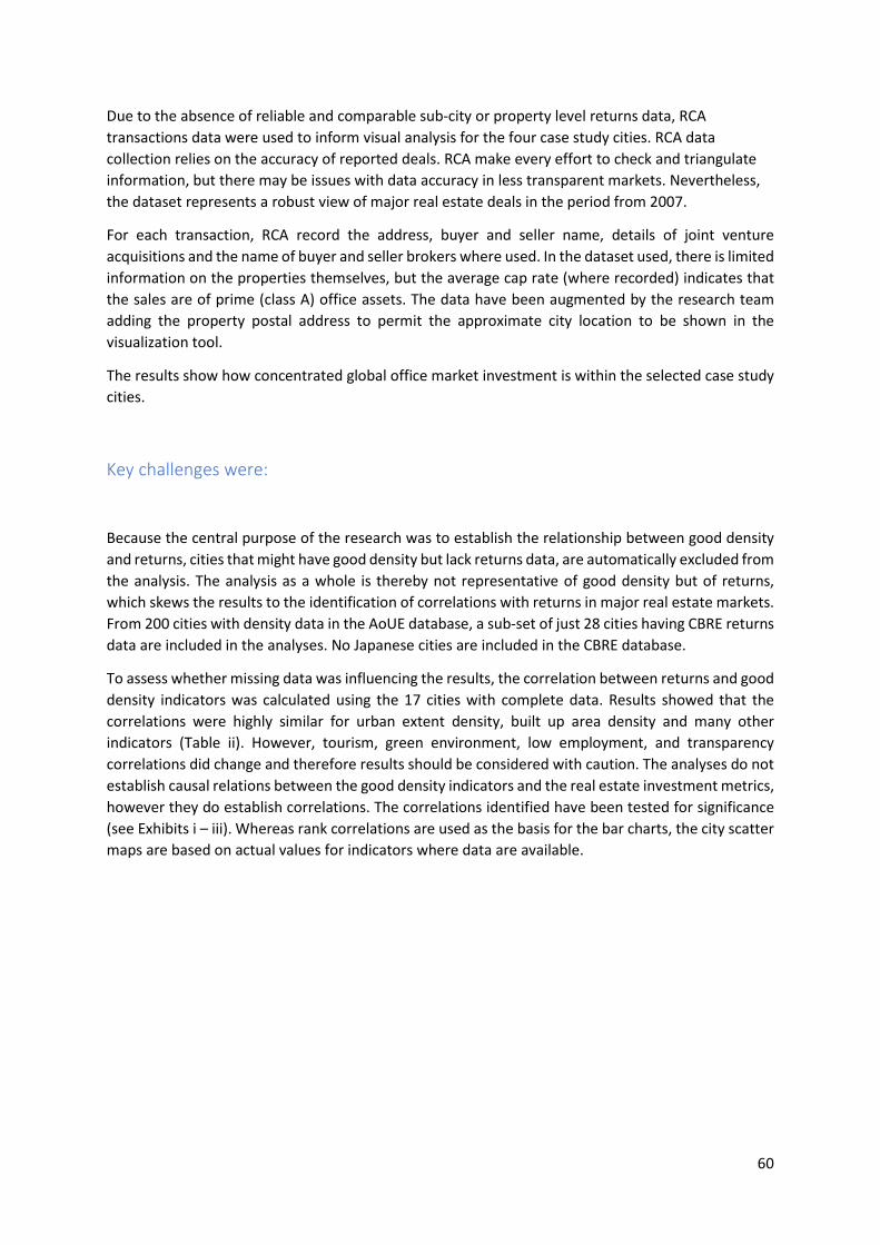
60
Due to the absence of reliable and comparable sub-city or property level returns data, RCA
transactions data were used to inform visual analysis for the four case study cities. RCA data
collection relies on the accuracy of reported deals. RCA make every effort to check and triangulate
information, but there may be issues with data accuracy in less transparent markets. Nevertheless,
the dataset represents a robust view of major real estate deals in the period from 2007.
For each transaction, RCA record the address, buyer and seller name, details of joint venture
acquisitions and the name of buyer and seller brokers where used. In the dataset used, there is limited
information on the properties themselves, but the average cap rate (where recorded) indicates that
the sales are of prime (class A) office assets. The data have been augmented by the research team
adding the property postal address to permit the approximate city location to be shown in the
visualization tool.
The results show how concentrated global office market investment is within the selected case study
cities.
Key challenges were:
Because the central purpose of the research was to establish the relationship between good density
and returns, cities that might have good density but lack returns data, are automatically excluded from
the analysis. The analysis as a whole is thereby not representative of good density but of returns,
which skews the results to the identification of correlations with returns in major real estate markets.
From 200 cities with density data in the AoUE database, a sub-set of just 28 cities having CBRE returns
data are included in the analyses. No Japanese cities are included in the CBRE database.
To assess whether missing data was influencing the results, the correlation between returns and good
density indicators was calculated using the 17 cities with complete data. Results showed that the
correlations were highly similar for urban extent density, built up area density and many other
indicators (Table ii). However, tourism, green environment, low employment, and transparency
correlations did change and therefore results should be considered with caution. The analyses do not
establish causal relations between the good density indicators and the real estate investment metrics,
however they do establish correlations. The correlations identified have been tested for significance
(see Exhibits i – iii). Whereas rank correlations are used as the basis for the bar charts, the city scatter
maps are based on actual values for indicators where data are available.

61
Table ii Correlations between returns and good density indicators when using only cities (N = 17)
with complete data.
Correlation with
returns
Real investment capital flows 0.21
Business services 0.45
Financial services 0.59
Innovation 0.20
Green environment 0.02
Transparency -0.07
Urban extent density 2016 0.72
Built up area density 2016 0.70
Open space ratio -0.19
Walkability ratio 2016 -0.41
Tourism 0.56
Low unemployment -0.20
Low crime 0.24
Table iii Correlations between capital flows and good density indicators when using only cities (N = 17) with complete data.
Correlation with
Real investment
capital flows
Returns 0.21
Business services 0.72
Financial services 0.74
Innovation 0.74
Green environment 0.20
Transparency 0.40
Urban extent density 2016 -0.19
Built up area density 2016 -0.23
Open space ratio 0.03
Walkability ratio 2016 -0.22
Tourism 0.28
Low unemployment 0.16
Low crime -0.16
62
D. Carbon emissions: Approach and challenges encountered
A review of relevant literature highlighted the critical importance of infrastructure development in
defining, as opposed to simply modifying, urban climate, emissions and air quality that impact on
environmental and human health. Integrated interdisciplinary research is needed to quantitatively
assess interactions across scales leading to different outcomes.
In relation to CO2 emissions specifically, the review also revealed that calculation is subject to different
methodological approaches that lead to differences in data reported globally, and its interpretation.
Consequently, although there is much evidence that increases in urban density are associated with
decreases in local, direct per capita CO2 emissions and energy consumption from motor vehicles and
buildings, there is debate about the overall magnitude and exact causal mechanisms of this
correlation.
General availability and quality of carbon emissions data
Different methods of CO2 accounting and data collection reflect two distinctive conceptual
approaches to the attribution of CO2 emissions linked to the scale of analysis and the units of
analysis used. Density reported for cities at a global level can therefore be misleading.
• Importance of scale
The most important urban form related variable controlling traffic emissions is likely to be the
distance between places of residence and jobs and other activities (Ewing and Cervero, 2010).
Emissions may therefore be displaced to urban locations with high through-flows of traffic and/or
traffic congestion. Increasing urban density may also displace emissions away from urban areas
towards less-regulated areas, resulting in an overall increase in emissions (Glaeser and Kahn, 2010;
Echinique et al., 2012). Because of this, either consumption- or production-based approaches to
emissions calculation may be used and this will be reflected in reported data.
• Importance of unit of analysis -
Typically, either per area or per capita emissions are reported. But, as population and built density
increase, per capita local CO2 emissions tend to decrease, whereas per area local emissions increase
(Christen. 2014; Kennedy et al., 2015) affecting the data reported. Furthermore, smaller dwelling
sizes associated with high population density tend to reduce per capita energy consumption, but
evidence suggests that after a certain unit size, high-rise apartment buildings tend to become less
energy/ CO2 efficient than low-rise or semi-detached homes (Rickwood et al., 2008; Van der Laan,
2011). Other variations in the units of analysis used include per unit area of living space (Norman et
al., 2006). The use of different units can lead to confusion in reporting practices and/or to mis-
interpretation of results.

63
Findings on availability of carbon emissions data:
Due to the problems with inconsistent methods and reporting practices at the global level of
analysis, after detailed exploration it was concluded that none of the sources available are of
sufficient quality to be usable.
The intention therefore was to use CO2 satellite data to allow global analysis.19 However the
technology is not yet mature enough. Data sources were found to have large gaps, to cover a
wide range of seasons, e.g. source vs sink variations, summer vs winter behaviour.
Unfortunately, this means that this independent and consistent data for all cities was not usable.
For example, even for London, satellite data are not usable (as they are often only partially
available). In consequence, a small sample of eight cities shown to have relevance for the
relationship between good density and real estate investment, were studied to scope the
availability and comparability of their data to inform investigation at case study city level (Table
iii).
Table iv Summary of CO2 sources.
City Data Link Notes Period
London Municipal
Inventory1
City- and borough level CO2e by sector and fuel type 2012
New York Municipal
Inventory2 City level CO2e by sector and fuel type 2014
Shanghai -Sugar et al.3
-World Bank
Report4
-Research paper, city level CO2e & emissions factors
-City level total and per capita CO2e emissions (p. 67)
-2006
-2006
Brussels -Municipal
Inventory5
-World Bank4
-City level CO2e, by sector
-City level total and per capita CO2e emissions (p. 25)
-1990-
2010
-2005
Berlin -CDP6
-World Bank4 -City level CO2e using a consumption based approach
-City level total and per capita CO2e emissions,
estimated from national level statistics (p. 68)
-2013
-2006
Warsaw -CDP6
-World Bank4 -City level total CO2 CO2e
-City level total and per capita CO2e emissions,
estimated from national level statistics (p. 68)
-2011
-2006
Zürich CDP6
City level total CO2e
2013
Hong
Kong
World Bank4 City level total and per capita CO2e emissions,
estimated from national level statistics (p. 68)
2006
Sources:
19 The advantages of CO2 observations from satellites are i) application of a consistent measurement
technique across all locations and ii) observed concentrations represent an integrated response from all sources and sinks (including vegetation and soils) across multiple scales. The disadvantages are i) limited
temporal coverage and ii) CO2 concentrations by themselves are not a direct measurement of emissions.
There are several techniques to derive emissions from concentrations, however, including analysis of vertical profile concentrations, inverse atmospheric modelling, or comparison with surrounding non-urban locations.
64
1Greater London Authority (2012) https://data.london.gov.uk/dataset/leggi2012, Accessed 13 Feb. 2017 2 The City of New York (2014) http://www1.nyc.gov/assets/sustainability/downloads/pdf/publications/NYC_GHG_Inventory_2014.pdf, Accessed 13 Feb. 2017 3 Sugar, L., Kennedy, C. and Leman, E. "Greenhouse gas emissions from Chinese cities." Journal of Industrial Ecology, 16.4 (2012): 552-563. http://onlinelibrary.wiley.com/doi/10.1111/j.1530-9290.2012.00481.x/pdf, Accessed 13 Feb. 2017 4 World Bank (2010) http://siteresources.worldbank.org/INTUWM/Resources/340232-1205330656272/CitiesandClimateChange.pdf, Accessed 14 Feb. 2017 5 City of Brussels (2012) http://www.environment.brussels/state-environment/summary-report-2011-2012/climate/emissions-greenhouse-gases, Accessed 13 Feb. 2017 6 CDP (2013) https://data.cdp.net/Cities/Citywide-GHG-Emissions-2013/qznk-mn6r/data, Accessed 13 Feb. 2017
Carbon data for case study cities
Data were finally collected for four case study cities - London, Zürich, Hong Kong and New York.
The data available for London allowed CO2 emissions at borough level to be extracted to inform
visual analysis in a landscape context: https://data.london.gov.uk/dataset/leggi2012 revealing sub-
city variations associated in part with volume of traffic flow and/or congestion. Caveats to be aware
of are that, first, London was the only city studied that had readily available data to illustrate CO2
emissions across spatial scales and, second, as is the case for a number of other cities, the CO2
emissions shown for London do not take into account the influence of vegetation. Furthermore, the
data for Zürich are not compatible with those for the other three case study cities due to a different
CO2 accounting method being used in Zürich (see technical note below).
Despite concerns about the in-consistency of CO2 reporting at the global level it was decided to also
run an initial analysis of the relationship between CO2 emissions and real estate investment,
followed by an analysis of the relationship between CO2 emissions and urban density for cities at the
global level: urban extent and built up density, walkability and open space ratio.
With the caveat that data sources available at a global level are self-reported and unreliable for the
varied reasons already explained, the source incorporated for the ‘green environment’ rank data,
from Arcadis was used to provide direct insight into potential relationships between CO2 emissions
and urban form given the interesting positive and negative correlations revealed with real estate
investment returns, CDP: https://data.cdp.net/Cities/Cities-2015-Map/ufw9-sh2k. Total city-wide
emissions (metric tonnes CO2e) were used to calculate emissions/km2/person (i.e. total emissions
standardised by area and population).
Technical note – Understanding the Zürich anomaly
The methodology used in Zürich CO2 emissions data calculation and reporting demonstrates the
problem with different approaches and data used for different cities, and their inconsistency.

65
The 2000-Watt Society methodology (Marechal et al., 2005) used for Zürich is based on a concept of
‘sustainable development’ that uses two indicators: Primary energy demand and greenhouse gas
emissions.
The methodology is based on the final energy demand. Primary energy factors and GHG emission
coefficients are used according to the ecoinvent database (database with consistent and
transparent, up-to-date Life Cycle Inventory (LCI) data – www.ecoinvent.org/database/). However,
the grey energy of net imported other goods and services, is not included in the methodology as
there are no specific data available. The methodology does not include emissions from non-
energetic sources (e.g. landfills, waste water treatment).
Primary energy is defined as the total energy present in the original energy source, plus its grey
energy. The energy that reaches the customer, after all conversion and transmission losses, is called
final energy. In turn, only a part of this is actually used: the effective energy. The rest is lost as waste
heat. The basis for all calculations is the final energy demand.
The basis of the methodology is the ‘territorial principle’. It refers to the energy consumed in the city
area and the emissions which occur there. The energy sources grey energy and grey emissions are
also taken into account. The grey energy of net imported other goods and service is not included in
the 2000 Watt Society methodology due to a lack of specific data. However, the aim is to separately
calculate and indicate the grey energy of net imported other goods and services. All calculations in
regard to primary energy demand and greenhouse gas emissions are made with the balancing
program ECORegion (http://www.ecospeed.ch/).
This example illustrates the challenges for comparative analysis presented by inconsistent concepts
and methods applied. The grey energy is not appropriate in this context as it mixes what occurs in
the city with its cultural “footprint” (not to be confused with the source area footprint of a CO2
sensor).
Technical note – Australian city anomaly
When visualising the distribution of CO2 emissions per km2 per person, it was apparent that
Australian cities were outliers (Figure i). Why Australian cities appear as outliers on this metric is
unclear but it is likely a consequence of the small land area and population within Australian cities.
The correlation between CO2 emissions per km2 per person and good density metrics was consistent
when Australian cities were removed from the analysis (Table v).
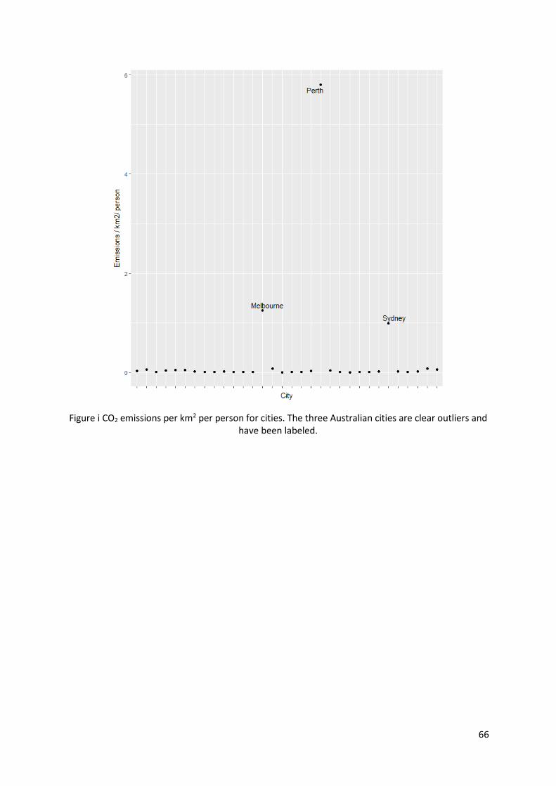
66
Figure i CO2 emissions per km2 per person for cities. The three Australian cities are clear outliers and have been labeled.

67
Table v Correlation between CO2 emissions per km2 per person and good density metrics excluding Australian cities.
Good density indicator
Correlation with
CO2 emissions per
km2 per person
p N
Returns after 2008 0.16 0.40 29
Real estate investment flows 0.33 8.97E-02 28
Business services 0.17 0.37 29
Financial services 0.14 0.48 29
Innovation 0.25 0.20 28
Low unemployment 0.29 0.20 21
Low crime 0.25 0.21 27
Green environment -0.02 0.91 27
Transparency -0.52 3.68E-03 29
Urban extent density 2016 0.30 0.26 16
Built up area density 2016 0.35 0.18 16
Open space ratio -0.31 0.24 16
Walkability ratio 2016 0.45 8.25E-02 16
Tourism 0.18 0.50 17
Key challenges were:
Additional to the challenges presented by a deficit of consistent data already discussed, there are
important specific data gaps for assessing relationships between CO2 emissions and urban density:
Transport emissions – Transportation which plays a critically important part in CO2 displacement
involving dense urban areas, may or not be included in assessment, dependent on the reporting
procedures adopted by governments for different cities.
City boundaries – City boundaries may not be consistent with other definitions being used
elsewhere in the analysis in this report.
Vegetation – Vegetation can offset some CO2 emissions but this is not being taken into account for
many, or most, analyses. This is important for comparative analysis, especially global analysis,
because cities have different growing seasons (e.g. high latitude vs low latitude), vegetation
amounts (e.g. London inner city vs residential London) etc., landscapes (soil and plant respiration)
can also emit CO2 and, again, this varies with climate (e.g. soil temperature). The role of green
infrastructure is not being considered.
Data gaps – In addition to inconsistencies due to data all being self-reported, not all relevant data is
necessarily available, for example, population, area, emissions.
Calculation methods are also inconsistent.
Bearing all challenges in mind, the database for global emissions was first checked for any city values
that were significantly different from the mean for cities worldwide. Australian cities were omitted

68
from subsequent correlation testing for this reason as their inclusion would have distorted the results
for all other countries.
NOTE: The University of Reading Meteorology research team are working on a model to remove
some of these problems to allow a consistent methodology to be used within a city. This is work that
could be expanded in future.
E. Transport Infrastructure Costs: Approach and challenges
encountered
Research focused on: (i) general availability and quality of urban transport infrastructure costs data
in order to inform selection of case study cities and methodological development and (ii) public
transport infrastructure cost and other data for four selected case study cities (London, Zürich, New
York and Hong Kong).
General availability and quality of transport infrastructure costs data
Research on availability and quality of public transport infrastructure costs data consisted of a rapid
review of known sources and other key sources resulting from key word searches. Due to time
limitations a more comprehensive literature search of transport and other infrastructure (ICT,
community services, green infrastructure, energy and water) was not undertaken. The transport
infrastructures included were road, rail, bus rapid transit (BRT), metro/underground, tram/light rail,
cycling and walking.
There are a large range of sources on the issue of transport infrastructure costs, from databases
(largely for benchmarking costs and international comparisons) and related studies, to city transport
authorities, academic studies and NGO websites and publications. Thus the challenge (at least in EU
and USA) was not lack of data in general on these infrastructure costs but rather availability of
comparable cost data per mode and appropriate level of detail at city level.
The most authoritative cost sources are city transportation authorities and related national and local
websites on infrastructure issues. City transportation authorities in general provide information on
budgets, planned and existing capital projects and a variety of other cost data. However, detailed
data on specific infrastructure costs is sometimes missing or difficult to find per project or mode of
transport (in some cases due to restricted public access including for commercial confidentiality
reasons where private contractors are used). Thus it may be appropriate to make direct contact
with selected city authorities for any further research.
The international databases reviewed are helpful in general reporting of typical cost ranges for
different types of infrastructures but often lack specific city data (as they are commonly intended to
guide planning through giving benchmark values), or have gaps in data or access restrictions. In the

69
absence of specific city cost data they could potentially be used to make ballpark estimates (or
indicative ranges) for transport infrastructure costs in combination with physical network data for
case study cities. However, caveats would be needed regarding validity of such data transfer to
study contexts.
It is common for the sources of detail on infrastructure cost to be given by specific mode (road, rail,
BRT, etc.) although urban transport authorities and key urban operators may also publish
consolidated costs data for the modes under their responsibility.
Comparability challenges can exist for infrastructure cost data between different modes of transport
due to different traditions in cost definitions, accounting practices and reporting. Thus it is necessary
to be clear and transparent where these differences exist, although in some reporting precise
definitions are not made explicit.
There are also potential comparability issues due to differences in the precise definitions and
accounting practices for reporting infrastructure costs between country contexts.
Findings on availability of infrastructure costs data per mode:
Roads: Indicative ranges of cost per km or per lane km for road infrastructure are available from a
range of sources (e.g. ROCKS, AICD, HM Treasury). There is a complex picture of different unit costs
available as these relate to different: (i) types of road including urban roads, (ii) types of costs (new
roads, renewal, routine maintenance and operational) and (iii) regions and countries. There is
commonly a large dispersion in unit costs for comparable road work activities.
Rail: Indicative average costs per km for rail infrastructure in Europe and USA are available. As with
roads there is a complex picture according to location, type of rail (high speed, commuter, light rail)
and type of cost, with a large dispersion in unit costs for comparable rail network activities.
Restricted access to key database for railway costs in Western European countries (Lasting
Infrastructure Cost Benchmarking (LICB)).
Metro: Infrastructure costs for Metro can vary even more widely than overground rail depending on
design factors and local conditions. The rapid review found reasonably good coverage of metro costs
in most selected cities.
Tram and Light Rail Transit: As in the case of rail and metro there are quite large variations in unit
costs for Tram and LRT for different locations. Average unit costs are available for EU countries and
USA.
Bus Rapid Transport: Detailed global evidence of BRT system costs is available (e.g. BRTData and
EMBARQ, 2013) although many gaps in data per city. Project costs vary significantly across systems
depending on design factors and local conditions. Typical ranges for capital costs of BRT are given as
$1m/km to 10m/km and for bus lanes as $1m/km to 5m/km (Rode et al, 2014).
Walking: Aggregate cost data on walking infrastructure can be more difficult to isolate than for other
modes as it may be included as part of road costs (for pavements), specific walkway projects and
cycle path projects. Some typical costs data are available.

70
Cycling: There are quite extensive general data available on urban cycling infrastructure in
developed countries. Although quantitative details on costs can be limited and some cities have
detailed infrastructure funding data, such as London. Typical cycle path capital costs are available.
A rapid review of general availability of public transport infrastructure cost sources for a small
selection of candidate cities for case studies was also undertaken. The key findings were:
- The most readily available cost data are for key Western European and North American
cities. London and New York have good general level of data for budgets and project
costs and a transparent reporting culture.
- Total cost data for Warsaw were available per transport mode. Although slightly more
difficult to track down and less detailed (than for London and New York) in the sources
reviewed, there is general reporting of funding and contractual arrangements.
- From the rapid review, reporting of transport funding and cost data in Shanghai seems
to be more limited.
- In terms of availability of cost data, Mumbai (and other Indian cities) seems to be a more
promising choice for an developing economy case study.
It was concluded that the costs most apposite at the city scale and feasible to include are as follows:
- Renewal and maintenance cost and operating costs per transport mode.
- Per km costs by transport mode. If not available a ballpark range could be estimated
given appropriate data availability on length of networks.
- Per resident or passenger costs by transport mode. If not available ballpark figures can
be estimated based on population, ridership and infrastructure cost totals.
The rapid review found very limited specification of infrastructure costs in relation to urban form. If
studies differentiate at all in infrastructure costs it is usually only between different sub categories
(e.g. motorway/trunk road/local road) rather than in spatial terms or urban forms. There is plenty of
evidence of variations in unit costs between different cities but in general this does not focus on
analyzing this according to urban forms.
Public transport data for case study cities
As for CO2 emissions, data were finally collected on public transport infrastructure for the four case
study cities of London, Zürich, Hong Kong and New York. Key sources were city transport authorities
and key operating company reports and websites, and other related reports. Key metrics researched
per transport mode were passenger numbers, numbers of routes, operating costs and capital costs
(renewal and maintenance). The organizational and funding context of public transport in the cities
was also established along with statistics on public transport’s share of the city’s transport market.
An estimation of operating expenditure per passenger for key public transport modes in each city
was made to the extent feasible with available data (Table vi).
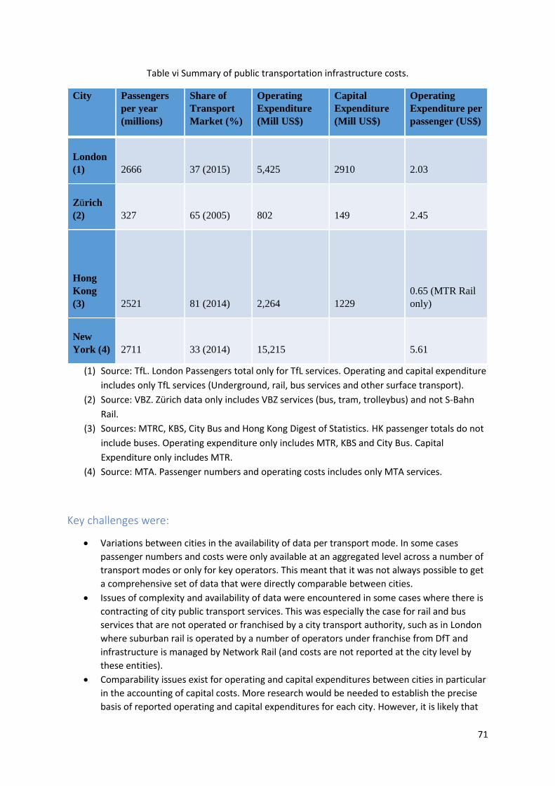
71
Table vi Summary of public transportation infrastructure costs.
City Passengers
per year
(millions)
Share of
Transport
Market (%)
Operating
Expenditure
(Mill US$)
Capital
Expenditure
(Mill US$)
Operating
Expenditure per
passenger (US$)
London
(1) 2666 37 (2015) 5,425 2910 2.03
Zürich
(2) 327 65 (2005) 802 149 2.45
Hong
Kong
(3) 2521 81 (2014) 2,264 1229
0.65 (MTR Rail
only)
New
York (4) 2711 33 (2014) 15,215 5.61
(1) Source: TfL. London Passengers total only for TfL services. Operating and capital expenditure
includes only TfL services (Underground, rail, bus services and other surface transport).
(2) Source: VBZ. Zürich data only includes VBZ services (bus, tram, trolleybus) and not S-Bahn
Rail.
(3) Sources: MTRC, KBS, City Bus and Hong Kong Digest of Statistics. HK passenger totals do not
include buses. Operating expenditure only includes MTR, KBS and City Bus. Capital
Expenditure only includes MTR.
(4) Source: MTA. Passenger numbers and operating costs includes only MTA services.
Key challenges were:
• Variations between cities in the availability of data per transport mode. In some cases
passenger numbers and costs were only available at an aggregated level across a number of
transport modes or only for key operators. This meant that it was not always possible to get
a comprehensive set of data that were directly comparable between cities.
• Issues of complexity and availability of data were encountered in some cases where there is
contracting of city public transport services. This was especially the case for rail and bus
services that are not operated or franchised by a city transport authority, such as in London
where suburban rail is operated by a number of operators under franchise from DfT and
infrastructure is managed by Network Rail (and costs are not reported at the city level by
these entities).
• Comparability issues exist for operating and capital expenditures between cities in particular
in the accounting of capital costs. More research would be needed to establish the precise
basis of reported operating and capital expenditures for each city. However, it is likely that

72
cost definitions and accounting practices differ to some extent between cities. It is possible
that some costs such as for maintenance and renewal are included as operating costs in
some instances and capital costs in others. In the case of New York it seems likely that
renewal and maintenance expenditures are included in the quoted operating costs as these
are much higher than for the other cities (in total and per passenger) and no separate figures
were found for these expenditures. Investment in major new infrastructure (new routes,
stations, etc.) was excluded from our research at present because a snapshot of costs in one
year or planning period was not considered meaningful in the context of city comparisons.
In consequence, it was only possible to report public transport costs at the city level. Further
research and consultation would be necessary to establish whether costs can be estimated with
greater granularity (e.g. per route/district/borough/fare zone).
Public transportation systems case study insights
London
Outline
Transport for London is responsible for managing a part of the city’s rail networks including the
London Underground, London Overground, Docklands Light Railway and TfL Rail, as well as bus, tram
and river services. The responsibility for operation of TfL managed services varies between modes
including wholly owned subsidiary companies (London Underground), private sector franchisees
(other rail services, trams and most buses) and licensees (river services and some buses). Other
(non- TfL) suburban rail services are part of the national rail network and are currently run by nine
Train Operating Companies (TOCs) under franchise contracts awarded and managed by DfT20
running on rail infrastructure managed by Network Rail. Public transport (Bus, tram, rail)
constituted 37 percent of all journeys in 2015, an increase of 9 percent since 2000 (TfL, 2016b).
Cost Data
Operating and capital costs for TfL managed services are given in their Budget and Business Plan
report (TfL 2016). Key points/caveats are:
• Total operating costs given in TfL accounts including Underground, Rail and Bus were
£2832m in 2015/6. The total including “other surface transport” was £3,660m but note that
while this will include other public transport modes (such as tram and ferry boat services) it
may also include non public transport services (e.g. cycling networks and taxi licences).
• In the above total bus operating costs are given as £84m but this is likely to include only TfL
management functions. A significant part of operating costs will be borne by franchised bus
companies. We do not have these figures (though a total could be calculated if operating
20 Plans to transfer responsibility for franchising all of London inner suburban rail services from the DfT to TfL were announced in 2016 (DfT/TfL, 2016) although currently there is some doubt about this transfer. https://www.ft.com/content/a7cbe84e-b1a7-11e6-9c37-5787335499a0

73
costs are available at the level of London services in the accounts of the various bus
operating companies) but note that a significant portion of the “Bus contract costs and ticket
commission” of £2,036m given in TfL accounts may be paid by contracted bus operating
companies in operating costs.
• Capital costs including Underground, Rail (TfL managed) and Bus were given as £1618m in
2015/6. Including “other surface transport” the total was £1,963m but the same caveat
regarding possible inclusion of some non public transport services applies here.
• New capital investment was £2,665m in 2015/6. A large part of this was for the major new
investment in Crossrail (£1,535m in 2015/16) which TfL is responsible for commissioning
jointly with the Department for Transport (DfT).
• There are difficulties in establishing operating costs for national rail services (i.e. non TfL
services) in London due to: (i) the lack of reporting of costs at the level of Greater London
since services are operated by Train Operating Companies (TOCs) to and from destinations
beyond London borders and (ii) the number of TOCs operating suburban services in London.
This is a significant omission given the large numbers of commuters using suburban rail
services. (I will keep looking for any available estimates)
• Establishing total capital costs for non TfL rail services in London is also problematic.
Renewal and maintenance for the national rail system rail is the responsibility of Network
Rail but costs are not reported at London level but according to eight regions of which six
connect to London (ORR, 2017).
Zürich
Outline
Zürcher Verkehrsverbund (ZVV) is the Canton of Zürich public transport authority responsible for
strategic planning, coordination and financing public transport. It provides the tariff and ticketing
system for public transport services but does not operate these services which are contracted to a
number of transport companies. Key operators in the City of Zürich are Verkehrsbetriebe Zürich
(VBZ) which operates trams, trolleybuses, buses, and funiculars and Zürich S-Bahn (rail system). The
Zürich public transport system maintains a high market share with 65 per cent (Moglestue 2005).
Cost Data
Total operating and capital costs are given in ZVV21 and VBZ sources22 for 2015. Key points/caveats
are:
• Total operating costs for transport companies in the Canton of Zürich calculated from ZVV
sources are CHF 721.8m. This includes labour costs and operating charge of transport
companies. The total operating charge for VBZ is given as CHF 516.5m.
• It is rather unclear whether the above total operating cost figure for ZVV includes S-Bahn as
one of the transport companies as there is an additional cost item of “Compensation to SBB
21 http://www.zvv.ch/zvv/en/about-us/zuercher-verkehrsverbund/figures-and-statistics/key-financial-figures.html 22 https://www.stadt-zuerich.ch/vbz/en/index/vbz/facts_figures/finances.html
74
and others” given in the ZVV summary which may refer to S-Bahn operating costs. If so, the
total operating cost would be CHF 794.4m.
• Zürich S Bahn covers the entire canton of Zürich and portions of neighbouring cantons. Thus
costs data for S Bahn may not be only for the city of Zürich.(To be clarified if possible)
• Total capital costs of transport companies are given as CHF 147.3m. Again it is not clear
whether this includes the S Bahn.
Hong Kong
Outline
The public transport system in Hong Kong includes Mass Transit Rail (MTR), light rail, tramways,
furnicular, bus, minibus, ferry and escalators systems. Transport Department of the Government of
Hong Kong is responsible for licensing of rail and bus operators in Hong Kong. A key operator is the
MTR Corporation with a 48.5 percent share of franchised transport market in Hong Kong (operating
the mass transit rail network and other rail and bus services). MTRC is an unusual example a
provider of city public transport covering the full costs and making a profit, achieved by the use of a
value-capture model (UNHabitat, 2013). The Kowloon Motor Bus Company (KBS) has a 24 per cent
share of the transport market while a number of other companies also operate transport services
(bus, tram, ferry, etc.). Public transport (Bus, tram, rail) constitutes 81 percent of all journeys (LTA,
2014).
Cost Data
The number of public transport operators makes establishing total operating and capital costs a
complex task and thus totals given only include the key operators and are therefore underestimates.
Cost totals have been calculated from data given in the financial reports for the main operators
(MTRC 2015, KBS 2015, City Bus 2016). Key points/caveats are:
• The value of 17.5 billion HK$ for total operating costs in 2015/6 includes MTRC, KBS and City
Bus Hong Kong transport operations only. Thus it does not include trams, ferries and
escalators and some buses and minibuses.
• A figure of 9.5 billion HK$ has been calculated for capital expenditure based on MTRC Hong
Kong operations only in 2015/6. Capital costs are not stated in bus operating company
reports we have reviewed and it is likely that routine capital costs (maintenance and
renewals) are included in the reported operating costs totals in these companies.
New York
Outline

75
The Metropolitan Transportation Authority (MTA) is responsible for operating most of New York
City's transit systems including subway, other rail and buses. A few services are run by other
operators (e.g. Staten Island Rail and Ferry) but most passenger and cost data are captured in the
MTA operations. Public transport (Bus, tram, rail) constitutes 33 percent of all journeys (LTA, 2014).
Cost Data
Sources for cost total are MTA financial reports (MTA 2017) and summaries23. Key points/caveats
are:
• The value of US$ 15.3 billion for total operating costs in year ending Dec 2015 includes MTA
operations (subway, rail, bus) and Staten Island Railway.
• We have yet to establish an annual figure for capital costs. Note that a separate company
“MTA Capital Construction” serves as the construction management company for MTA
expansion projects and mobility projects. Projects includes major investments in transport
infrastructure included hubs (e.g. The Fulton Centre).
• Further discussion of capital investment needs for public transit in New York can be found in
the report by ASCE (2015) which concludes that: “upstate and suburban transit systems
require $1 billion over the next five years to maintain infrastructure in a state of good repair
and add capacity to address ridership demand. However, the anticipated funding will only
cover 43% of transit infrastructure needs, leaving a $577 million funding gap”.
Sources: AICD: Africa Infrastructure Country Diagnostic. http://data.worldbank.org/data-catalog/africa-infrastructure City Bus (2016), City Bus Fuller Disclosure http://www.nwstbus.com.hk/_common/pdf/CitybusFuller2016.pdf DfT/TfL (2016) A New Approach to Rail Passenger Services in London and the South East. Department for Transport and Transport for London. https://www.gov.uk/government/uploads/system/uploads/attachment_data/file/493754/dft-tfl-rail-prospectus.pdf EMBARQ (2013) Social, Environmental and Economic Impacts of BRT Systems: Bus Rapid Transit Case Studies from Around the World, report for EMBARQ a program of the World Resources Institute. HM Treasury (2010): Infrastructure Cost Review: Technical Report, led by Infrastructure UK, December 2010. KBS (2015) More about KBS 2015 http://www.kmb.hk/chi/pdf/moreKMB.pdf LICB: Lasting Infrastructure Cost Benchmarking. http://transport-research.info/project/lasting-infrastructure-cost-benchmarking-database LTA (2011) Journeys: Sharing Urban Transport Solutions, Issue 7, Nov 2011 Land Transport Authority Academy, Singapore. https://www.lta.gov.sg/ltaacademy/doc/JOURNEYS_Nov2011%20Revised.pdf LTA (2014) Journeys: Sharing Urban Transport Solutions, Issue 12, Nov 2014, Land Transport Authority Academy, Singapore. https://www.lta.gov.sg/ltaacademy/doc/Journeys_Issue_12_Nov_2014.pdf Moglestue, A. (2005) http://www.proaktiva.ch/tram/zurich/zurich05_0.html
23 http://web.mta.info/mta/network.htm

76
MTA (2017) MTA 2017 Adopted Budget, Metropolitan Transport Authority, Feb 2017. http://web.mta.info/mta/budget/pdf/MTA%202017%20Adopted%20Budget%20February%20Financial%20Plan%202017-2020.pdf MTRC (2015) MTRC Exec Management Report: HK Transport Operations 2015 http://www.mtr.com.hk/en/corporate/investor/2015frpt.html ORR (2017) UK Rail Industry Financial Information 2015-16, Office of Rail and Road, February 2017. http://orr.gov.uk/__data/assets/pdf_file/0020/24149/uk-rail-industry-financial-information-2015-16.pdf ROCKS: Road Costs Knowledge System. http://go.worldbank.org/ZF1I4CJNX0 TfL (2015) Rail and Underground International Benchmarking Report, Transport for London, Rail and Underground Panel TfL (2016a) TfL Budget 2016/17 and Business Plan March 2016, Transport for London. TfL (2016b) Travel in London: Report 9, Transport for London. http://content.tfl.gov.uk/travel-in-london-report-9.pdf UNHabitat (2013) Planning and Design for Sustainable Urban Mobility: Global Report on Human Settlements, United Nations Human Settlements Programme. https://unhabitat.org/planning-and-design-for-sustainable-urban-mobility-global-report-on-human-settlements-2013/
F. Significance heat charts
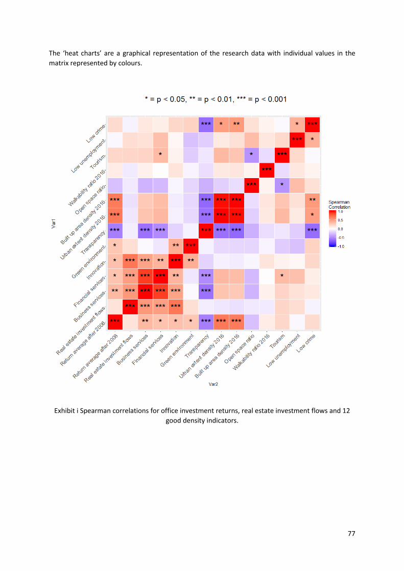
77
The ‘heat charts’ are a graphical representation of the research data with individual values in the
matrix represented by colours.
Exhibit i Spearman correlations for office investment returns, real estate investment flows and 12
good density indicators.
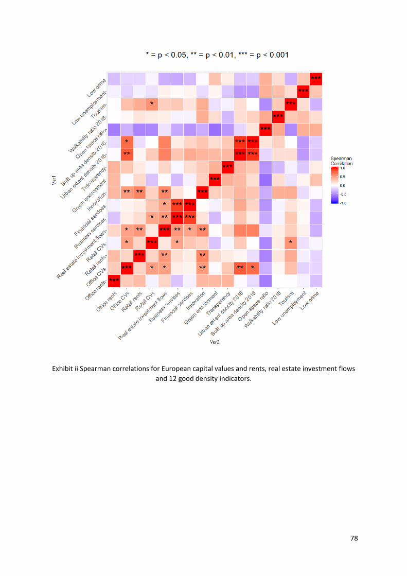
78
Exhibit ii Spearman correlations for European capital values and rents, real estate investment flows
and 12 good density indicators.

79
Exhibit iii Spearman correlations between returns, real estate investment flows and 12 good density
indicators when only using cities with complete data.

80
G. List of references
Adams, D., Larkham, P. and Pain, K. (2015), Viewpoint: Re-evaluating the place of urban planning
history, Town Planning Review, 86(2), 373-379.
Akakandelwa, N., Devaney, S.and Pain, K. (2016) Social networks and sales transactions in South
African office market, 16th AfRES Annual Conference, Kara, A. (ed.), pp. 291 – 312. Addis
Ababa, Ethiopia: African Real Estate Society.
Angotti, T. (2006) Apocalyptic anti-urbanism: Mike Davis and his planet of slums, International Journal
of Urban and Regional Research, 30, 961-967.
Barlow, J. et al. (2017) Developing a research strategy to better understand, observe and simulate
urban atmospheric processes at kilometre to sub-kilometre scales, Bulletin of the American
Meteorological Society, DOI: 10.1175/BAMS-D-17-0106.1:
http://journals.ametsoc.org/doi/abs/10.1175/BAMS-D-17-0106.1.
Blowers, A. and Pain, K. (1999) The Unsustainable City? Understanding Cities: Unruly Cities?
Order/Disorder, Pile, S., Brook, C. and Mooney, G. (eds.), pp. 247-298. London: Routledge.
Braun, B. (2006) Environmental issues: global natures in the space of assemblage, Progress in Human
Geography, 30, 5, 644-654.
Bridge, G. (2009) The hole world: scales and spaces of extraction, New Geographies, 2, 43-49.
Castells, M., Hall. P. and Pain, K. (2007) Centrality in the Space of Flows, Built Environment, 33(4), 482-
485.
Christen, A. (2014) Atmospheric measurement techniques to quantify greenhouse gas emissions
from cities, Urban Climate, 10, 241‐260.
Clark, G. and Moir, E. (2015) Density Drivers, Dividends and Debates, June. London: Urban Land
Institute.
Clark, G. and Moonen, T. (2005) The Density Dividend: solutions for growing and shrinking cities,
October. London: Urban Land Institute.
Cochrane, A. and Pain, K. (2004) A Globalising Society? A Globalising World? Culture, Economics,
Politics, Held, D. (ed.), pp. 5-45. London: Taylor & Francis Ltd.
Cook, G.A.S., Pandit, N.R., Beaverstock, J.V., Taylor, P.J., Pain, K. (2007) The role of location in
knowledge creation and diffusion: evidence of centripetal and centrifugal forces in the City of
London financial services agglomeration, Environment and Planning A, 39(6), 1325-1345.
Cushman Wakefield (2016) Personal communication for presentation to the Association of IT &
Business Process Services (ASPIRE) Annual Conference, Krakow, Poland, The Dragon Wakes,
11th – 12th May, 2016.
Davis, K. (1965) The urbanisation of the human population, Scientific American, September.
Davis, M. (2006) Planet of Slums. New York: Verso.
Dawson, J.A. (Ed.) (2012) Retail Geography, Volume 7. London & New York: Routledge.

81
DEFRA/DoT (Department for Environment, Food & Rural Affairs/Department for Transport) (2017)
Improving air quality in the UK: tackling nitrous oxide in our towns and cities. London: Office
for National Statistics.
Echenique, M.H., Hargreaves, A.J., Mitchell, G. and Namdeo, A. (2012) Growing cities sustainably: does
urban form really matter? Journal of the American Planning Association, 78(2), 121-137.
Epifani, I. and Nicolini, R. (2017) Modelling population density over time: how spatial distance matters,
Regional Studies, 51(4), 602-615.
Ewing R. and Cervero, R. (2010) Travel and the built environment, Journal of the American Planning
Association, 76(3), 265‐294.
Florida, R., Adler, P. and Mellander, C. (2017) The city as an innovation machine, Regional Studies,
51(1), 86-96.
Foster (2010) J., Lowe, A. and Winkelman, S. (2011) The value of green infrastructure for urban
climate adaptation.Washington DC: Centre for Clean Air Policy.
Fuertz, F., Milcheva, S. and Baum, A. (2015) Cross-Border Capital Flows into Real Estate, Real Estate
Finance, 31(3), 103-122.
Glaeser and Saiz (2003) The Rise of the Skilled City. Harvard Institute of Economic Research. Discussion
Paper no. 2025. Cambridge Massachusetts: Harvard [WWW] Available from:
https://scholar.harvard.edu/glaeser/publications/rise-skilled-city.
Glaeser, E.L. and Gottlieb, J. (2009) The Wealth of Cities: Agglomeration Economies and Spatial
Equilibrium in the United States. Cambridge Massachusetts: Harvard University. [WWW]
Available from: https://scholar.harvard.edu/glaeser/publications/wealth-cities-
agglomeration-economies-and-spatial-equilibrium-united-states.
Glaeser E.L. and Kahn, M.E. (2010) The greenness of cities: carbon dioxide emissions and urban
development, Journal of Urban Economics, 67(3), 404-418.
Graham, S. and McFarlane, C. (2015) Infrastructural lives: urban infrastructure in context. London:
Routledge-Earthscan.
Guagliardo, M. (2004) Spatial accessibility of primary care: concepts, methods and challenges,
International Journal of Health Geographics, 3(3). [WWW] Available from: https://ij-
healthgeographics.biomedcentral.com/articles/10.1186/1476-072X-3-3.
Hall, P. and Pain K. (eds.) (2006) The Polycentric Metropolis: Learning from mega-city regions in Europe,
Earthscan: London.
Harrison, J. and Pain, K. (eds.) (2012) Global Cities, Volume IV: Planning and Governance of Cities in
Globalization, Routledge: London.
Henneberry, J. and Mouzakis, F. (2014) Familiarity and the Determination of Yields for Regional Office
Property Investments in the UK, Regional Studies, 48 (3), 530-546.
Keil, R. (2014) Sub/urbanisation and density: A few critical notes, Global Suburbainsms: Governance,
Land and Infrastructure in the 21st Century. [WWW] Available from:
http://suburbs.apps01.yorku.ca/2014/02/14/suburbanization-and-density-a-few-critical-
notes/#sthash.X1wnr0QJ.dpuf.
82
Kennedy C.A., Stewart, I., Facchini, A., Cersosimo, I., Mele, R., Chen, B., Uda, M., Kansal, A., Chiu, A.,
Kim, K.G. and Dubeux, C.(2015) Energy and material flows of megacities, Proceedings of the
National Academy of Sciences, 112(19), 5985‐5990.
Lizieri, C. (2009) Towers of Capital: Office Markets and International Financial Services. Oxford: Wiley-
Blackwell.
Lizieri, C. and Pain, K. (2014) International Office Investment in Global Cities: The Production of
Financial Space and Systemic Risk, Regional Studies, 48 (3), 439-455.
Lizieri, C., Pain. K. and Vinciguerra, S. (2012) Real Estate Investment Flows, Working Paper 9, TIGER
Territorial Impact of Globalization for Europe and its Regions, Applied Research 2013/1/1,
February. Brussels: European Spatial Observation Network. [WWW] Available from:
http://164.15.12.207/espon/tiger/final/.
Mahroum, S., Huggins, R., Clayton, N., Pain, K. and Taylor, P.J. (2008), Innovation by Adoption:
Measuring and Mapping Absorptive Capacity in UK Nations and Regions, October. London:
National Endowment for Science, Technology and the Arts. [WWW] Available from:
http://www.nesta.org.uk/assets/Uploads/pdf/Research-
Report/innovation_by_adoption_report_NESTA.pdf (electronic).
Mackenzie, D. (2008) Material Markets: How Economic Agents are Constructed. Oxford: Oxford
University Press.
Marechal, François, Daniel Favrat, and Eberhard Jochem (2005) Energy in the perspective of the
sustainable development: The 2000W society challenge, Resources, Conservation and
Recycling, 44(3), 245-262.
Martin, D. and Secor, A. (2014) Towards a post-mathematical topology, Progress in Human Geography,
38(3), 420-438.
McAllister, P. and Nanda, A. (2014) Which Factors Determine Cross-Border Real Estate Capital Flows?
A Gravity Modelling Approach, working paper.
McGhee, G., Glenn. R. and Atkinson, J. (2007) Grounded theory research: Literature reviewing and
reflexivity, JAN, 60(3), 334-342.
Milcheva, S. and Zhu, B. (2016a) Asset Pricing, Spatial Linkages and Contagion in Real Estate Stocks,
paper under review.
Milcheva, S. and Zhu, B. (2016b) The Pricing of Spatial Linkages in Companies’ Underlying Assets,
working paper.
Milcheva, S. and Zhu, B. (2016c) Spatial Dependence in Asset Pricing Models, paper under review.
Nayak, J., Naik, B. and Behera, H.S. (2014) Fuzzy C-Means (FCM) clustering algorithm: A decade review
from 2000 to 2014, Computational Intelligence in Data Mining, 2, 133-149.
Neuwirth, R. (2006) Shadow Cities: A Billion Squatters, A New Urban World. New York: Routledge.
Norman J., MacLean, H.L. and Kennedy, C.A. (2006) Comparing high and low residential density: life-
cycle analysis of energy use and greenhouse gas emissions, Journal of Urban Planning and
Development, 132(1), 10‐21.

83
Pain, K. (2006) Policy Challenges of Functional Polycentricity in a Global Mega-City Region: South East
England, Built Environment, 32(2), 194-205.
Pain, K. (2008a) Spaces of practice in advanced business services: rethinking London-Frankfurt
relations, Environment and Planning D: Society and Space, 26(2), 264-279.
Pain, K. (2008b) Examining Core-Periphery Relationships in a Global Mega-City Region - The Case of
London and South East England, Regional Studies, 42(8), 1161-1172.
Pain, K. (2012) Locational Investment: Where to target investment for maximum economic returns.
RICS Research, May. London: Royal Institution of Chartered Surveyors, [WWW] Available
from: http://www.rics.org/site/scripts/download_info.aspx?fileID=11938&categoryID=523.
Pain, K. (2016) Megaregions Imaginaries: Excursions through a maze, Geographical Review, 106(2),
Available from: http://onlinelibrary.wiley.com/doi/10.1111/j.1931-0846.2016.12171.x/full.
Pain, K. (2017) Land Use Policy and Governance of Real Estate Development, Routledge Real Estate
Companion, Squires, G., Heurkens, E. and Peiser, R. (eds.), unpublished, in press.
Pain, K. and Hall, P. (2008) Informational Quantity versus Informational Quality: The perils of
navigating the space of flows, Regional Studies, 42(8), 1065-1077.
Pain, K. and Van Hamme, G. (2014) Changing Urban and Regional Relations in a Globalizing World:
Europe as a Global Macro-Region, Edward Elgar, Cheltenham.
Pain, K. and Van Hamme, G. and Vinciguerra, S. (2015) Global networks, cities and economic
performance: Observations from an analysis of cities in Europe and the US, Urban Studies,
53(6), 1137-1161.
Pain, K., Vinciguerra, S., Hoyler, M., Taylor, P.J. (2012) Europe in the World City Network, Working
Paper 3, TIGER Territorial Impact of Globalization for Europe and its Regions, Applied
Research 2013/1/1, European Spatial Observation Network, Brussels, February. [WWW]
Available from: http://164.15.12.207/espon/tiger/final/.
Rapoport, A. (1975) Toward a redefinition of density, Environment and Behaviour, 2(2), 133-157.
Rickwood P., Glazebrook, G. and Searle, G. (2008) Urban structure and energy—a review, Urban
Policy and Research, 26(1), 57-81.
RTPI (Royal Town Planning Institute) (2017) Planning central to improving air quality, The Planner,
June, London: Royal Town Planning Institute. [WWW] Available from:
https://www.theplanner.co.uk/news/rtpi-planning-%E2%80%98central%E2%80%99-to-
improving-air-quality?utm_source=Adestra&utm_medium=email&utm_term=
Sheller, M. (2004) Mobile publics: Beyond the network perspective, Environment and Planning D:
Society and Space, 22(1), 39-52.
Spearman C (1904) The proof and measurement of association between two things, American Journal
of Psychology, 15, 72–101.
Stevenson, S., Akimov, A., Hutson, E. and Krystalogianni, A. (2014) Concordance in Global Office
Market Cycles, Regional Studies, 48(3), 456-470.
Tang, X., Phillips, N., Nomack, M. Pasquarella, V. and Pitts, J. (2016) Computers, Environment and
Urban Systems, 57, 212-223.

84
Taylor, P.J., Beaverstock, J.V., Cook, G., Pandit, N., Pain, K. (2003) Financial Services Clustering and its
significance for London, February. Corporation of London, London. [WWW] Available from:
http://www.cityoflondon.gov.uk/NR/rdonlyres/1C75B813-796E-45F8-83A2-
7FD5D28D4F56/0/BC_RS_clustering_0302_XR.pdf (electronic).
Taylor, P.J., Evans, D. and Pain, K. (2008) Application of the Inter-Locking Network Model to Mega City-
Regions: Measuring Polycentricity within and beyond City-Regions, Regional Studies, 42(8),
1079-1093.
Tonkiss, F. (2014) Cities by Design: The Social Life of Urban Form. Cambridge: Polity Press.
United Nations (2017) World population Prospects: The 2017 Revision. New York: United Nations.
Wilson, M.W. (2014) Continuous connectivity, handheld computers, and mobile spatial knowledge,
Environment and Planning D: Society and Space, 32(3) 535-555.
Van der Laan M.T. (2011) Scaling urban energy use and greenhouse gas emissions through LiDAR,
M.Sc. dissertation, University of British Columbia. Adey, P. (2010) Aerial life: Spaces,
mobilities, affects. Oxford: Wiley-Blackwell.
Van Hamme, G., Pain. K. and Vinciguerra, S. (2012) Cities, Networks and Economic Performances: A
comparative study on European and US cities, Working Paper 4, TIGER Territorial Impact of
Globalization for Europe and its Regions, Applied Research 2013/1/1, European Spatial
Observation Network, Brussels, February 2012. [WWW] Available from:
http://164.15.12.207/espon/tiger/final/.
Zhu, B. and Milcheva, S. (2016) Spatial linkages in listed property returns in tranquil and distressed
periods, American Real Estate Society, 22(2) 129-146.

85
ANNEX II - Interview research key messages, ethics application
documentation and questionnaire proformas
Key messages from Steering Group member interviews
For background information on the interview ethics application, information sheet, signed consent
form and questionnaire proformas.
Research interest: Gain insights into future markets and marketable investments in relation to
good density / sustainability for diversification. To reflect changing population demographics,
employment, capital productivity, concentration, infrastructure, connectivity and economic growth,
and their relationship to property value, rental levels, liquidity and risk profiles. To increase market
knowledge, to identify marketable investment opportunities that meet different client expectations,
and to feed into forecasting and an appraisal tool.
Scale focus: Cross-border global, city-region, micro and property scales.
Analytical focus: Capital market allocations and investment strategy on value, risk and returns for
internal decision-making (global strategy, acquisitions, landscape level projects) and for marketing,
investor advice (responsible investment), public authority discussions and wider public-private sector
collaboration.
Geographical focus: Mature and developing markets: within Europe, prime markets, e.g. London,
Paris, Brussels, Amsterdam, Berlin. In developing markets: China, India, South America and Eastern
Europe, e.g. Poland.
Real estate sector focus: Offices (large cities / prime), retail and, if available, residential and non-
traditional property uses, e.g. business processing.
Methodological focus: Robust commercial quantitative market data, subject to data volume,
coverage, collection methodology and comparability. Quantitative urban form metrics where
possible, and a qualitative element for intuitive interpretation incorporating findings from the
international research reviewed to inform forecasting and underwriting, and sense check heuristic
social network information.
Expectations:
Practical recommendations from a high-level report with a forward-looking, global prime A-class
investment focus to consider a range influencing factors, including: What kinds of countries and
sectors to invest in? Where is marketable and where is secure for investors? Why do certain cities
have good density, e.g. population size, density threshold, land use linked to buildings, offices, balance
of green space, transport infrastructure, traffic generation, carbon and environmental change,
housing supply, location and affordability, amenities, cultural aspects, heritage, quality and design
principles? At functional urban region, city and sub-city levels, how do the following contribute to real
estate investment value and returns: economic growth, spatial structure, mixed-use, transport
infrastructure, commuting, walkability, green space, contiguity of physical development? What would
good density look like?

86
School of Real Estate and Planning Research Project Ethical Approval
Introduction
The University Research Ethics Committee has issued Guidance Notes outlining its Terms of Reference and procedures: http://www.reading.ac.uk/internal/res/ResearchEthics/reas-REethicshomepage.aspx In accordance with the Notes for Guidance, ethical propriety of all research relating to human subjects or human personal data must be assessed for undergraduate, masters, postgraduate and staff research projects. If project methods alter significantly subsequent to initial ethics clearance, then a new application form will need to be generated and approved.
Is it research? It is not research if the activity is carried out solely for the purpose of teaching and learning, or if it constitutes Clinical or Social work practice or audit. With regard to the latter two categories, see Annex E in the Guidance Notes (PDF-299kb). If the activity is not research, then it does not require ethical approval.
Is it research on human subjects, human samples or human personal data? If the answer to this question is "yes" then the research requires ethical approval, subject to the following questions:
If it involves human data, are those data in the public domain? Do they relate to
deceased persons?
If the answer to either of these questions is "yes", there is no need to obtain ethical approval; but ethical considerations may still be relevant.
If the answer to both these questions is "no", then ethical approval is needed.
Ethical concerns are usually strongest where data are gathered directly from the subject. If the project is funded by a Research Council or other external source then ethical clearance should be sought via the University Research Ethics Committee (see page 5).

87
The responsibility for ethical conduct of research in the School lies with the Head of School. Under the exceptions procedure outlined in the Notes for Guidance, REP’s Head of School (HoS) can approve research project ethical applications (see Annex 1). Authority to sign off ethical approval forms lies with the HoS or nominated persons. Students should discuss their applications with their supervisors prior to submitting to the HoS for approval. If the supervisor is not available, students should contact their Programme Director.
Procedure
Ethical review should be obtained before data collection or recruitment is initiated. This includes feasibility or pilot studies. This form should be completed by the student/member of academic staff as appropriate and submitted to the School Secretary.
• Ethics clearance must be obtained before the research project commences.
• There is an obligation on all students and academic staff to observe ethical procedures and practice, and raise any concerns or questions with the Head of School. If the Head of School is not available, please contact the Director of Research.
• Records will be maintained and audited as required by the University Research Ethics Committee.
• Completed Consent Forms must be retained by the School for a minimum period of five years from the date at which the project is completed. If ethical clearance is sought from a different School, a copy of the clearance must also be retained in REP.
• The storage of consent forms may be audited from time to time.
• This form is designed to conform to the University’s requirements with respect to research ethics. Approval under this procedure does not confirm the academic validity of the proposed project.
• Student research project ethical applications must be referred to the dissertation/thesis supervisor in the first instance for advice; however, sign off must be done by the HoS. Research projects requiring ethical clearance undertaken in the absence of this form will not be marked.
• If in the course of the work the nature of the project changes (including research methods and questionnaire), advice should be sought from the academic supervisor / Course Director and, if required, a further application form for ethical clearance submitted.
• Similarly, if appropriate, changes in the nature of staff research projects (including research methods and questionnaire), must be considered for re-submission for ethical clearance.
• The following must be submitted with this form for approval: • The information sheet (see Annex 2a and 2b)
• Consent form (Annex 3)
• (Survey) methods
• Questionnaires or surveys (if appropriate)
• Focus group or interview questions (if appropriate)

88
• Please allow sufficient time when seeking ethics approval. The following timescales are an indication:
• Head of School approval – 2 weeks
• University’s Research Ethics Committee – a minimum of 4 weeks

89
School of Real Estate and Planning Research Ethics Form
Title of Proposed Project: Supporting Smart Urban Growth: Successful Investing in Density
Project Details: The research is investigating how urbanisation can be made more sustainable through
improved private and public sector real estate investment decision-making
Name & email address of principle researcher/student: Professor Kathy Pain: [email protected]
Name and email address of supervisor (if applicable): NA
Date of commencement: August 15, 2016 Date of completion: January 31, 2017 (The application is being submitted now because the original project brief did not include collection of personal data.)
Project type (tick as appropriate):
*Staff research ✓ Masters
Undergraduate Doctoral Other ……………………………….. *Staff research projects should be signed off by the Director of Research or Head of School.
90
Brief Summary of Proposed Project and Research Methods
The research is investigating how urbanisation can be made more sustainable
through improved private and public sector real estate investment decision-
making. The approach is interdisciplinary and the geographical scope is global. A
model will be delivered which will enable real estate investors to make informed
investment decisions which will simultaneously improve their investment returns
whilst also investing in sustainable urban density and urban form. This work is
funded by industry investment via the Urban Land Institute in association with the
New Climate Economy (NCE). Together these organisations lead the way on
sustainable urban land use and the provision of robust evidence on actions which
both increase prosperity and resilience, whilst at the same time reduce the risks of
climate change.
There are two phases to the research: Phase I is a literature review of secondary
sources – scholarly research papers and grey literature – and data sources. A new
element of this research phase (not included in the original brief) is an interview
survey with relevant industry experts. The survey will help to inform the research
team on: (1) the ways in which the research will be used by industry and (2)
relevant information and data sources. In Phase II, relevant data will be analysed
and modelled.

91
Data Management
Research Data management is an important consideration within research ethics and is the sum of activities undertaken in relation to the collection, processing, retention and disposal of research data. Research data, by being well managed, can generate benefits for both the University and its researchers in terms of greater research impact, enhanced reputation, and increased return on investment. Further information on the University’s Research Data Management Policy can be found here here. Yes No
Have all aspects of Research Data Management been considered? See What is Research Data Management
✓
Active data will be stored on a secure University drive (NOT on computer/laptop hard drives) Tools and Services
✓
Have appropriate processes for the retention of data been considered? Tools and Services
✓
Will the University of Reading Research Data archive be used? ✓
For personal and sensitive data have measures been put in place to make data of long-term value accessible to the fullest extent that is consistent with any confidentiality requirements? Such measures might include using the initial consent process to secure broad consent for data sharing, and the use of anonymisation techniques, data aggregation, and editing of video or sound recordings to remove personal identifiers from data. The UK Data Archive has a comprehensive guide on consent and ethics
✓
For sensitive data (e.g. industry data) appropriate arrangements for what can and cannot be done with the data, and who may or may not have access to the data, are defined by participation agreements or the terms of contract.
✓
Where appropriate, arrangements for disposal of data have been made ✓
Appropriate training and/or information resources have been accessed Training and General Information
✓
PhD students have identified data management training (section C1 of the Learning Needs Analysis) and undertaken the necessary training through the Reading Researcher Development Programme (RRDP)
NA
Postgraduate and Masters students in Planning have taken the Research Methods Module (to be replaced by Good Academic Content Course/Workshop in Autumn 2017)
NA
Undergraduate Year 3 research module students have taken the Research Methods Module (to be replaced by Good Academic Content Course/Workshop in Autumn 2017)
NA

92
Health and Safety
Yes No
Will the research be conducted away from an office environment or normal place of work?
✓
Will the research be conducted outside normal working hours? please note the details below and comment on how the personal safety and security of the researcher(s) has been safeguarded:
✓
If you have answered “yes” to either of the above questions, please detail the steps taken to ensure the personal safety and security of the researcher(s)
Training needs in Health and Safety have been assessed ✓
Where appropriate, PhD students have identified Health and Safety training (section C1 of Learning Needs Analysis) and undertaken the necessary training through the Reading Researcher Development Programme (RRDP)
NA
Postgraduate and Masters students in Planning have taken the Research Methods Module (to be replaced by Good Academic Content Course/Workshop in Autumn 2017)
NA
Undergraduate Year 3 research module students have taken the Research Methods Module (to be replaced by Good Academic Content Course/Workshop in Autumn 2017)
NA

93
Checklist for Investigator
✓ I confirm that where appropriate a consent form and information sheet has
been prepared in accordance with the checklist and will be made available to all
participants. This contains details of the project, contact details for the principal
researcher and advises subjects that their privacy will be protected and that their
participation is voluntary and that they may withdraw at any time without reason.
✓ I confirm that research instruments (questionnaires, interview guides, etc)
have been reviewed against the policies and criteria noted in The University
Research Ethics Committee Notes for Guidance. Information obtained will be
safeguarded and personal privacy and commercial confidentiality will be strictly
observed in accordance with the University’s Data Management Policy
✓ I confirm that where appropriate a copy of the Consent Form and details of
the Research Instruments/Protocols are attached and submitted with this
application. Arrangements have also been made for the storage of the forms for a
minimum period of five years from the date of project completion.
NA For student research, I can confirm that I have consulted with my dissertation supervisor or Programme Director prior to submitting this form, and attended the necessary RRDP training courses.
Approval by HoS or nominee
I have reviewed this application as APPROVED and confirm that it is consistent
with the requirements of the University Research Ethics Committee procedures
This proposal is NOT APPROVED and is returned to the applicant for further consideration / revision.
This proposal is NOT APPROVED and will now be submitted to the University Research Ethics Committee
COMMENTS (e.g. where application has been refused): …………………………………………………………………………………………………..

94
Signed (Staff or Student Investigator): Date: 15 Oct 2016……………… Signed (HoS or nominee): …………………………………………Date: ……….……….

95
ANNEX 1
Exceptions
The HoS can approve Ethical Clearance applications with some exceptions. Please confirm whether your work falls within the exceptions process by answering the following:
Yes/Agree No
To the best of my knowledge the participants and subjects of the study are not patients or clients of the National Health Service (NHS) or social services.
✓
Participants and subjects of the study have the capacity to give free and informed consent within the meaning of the Mental Capacity Act 2005 to the best of my knowledge.
✓
Questions are not likely to be considered impertinent or to cause distress to any of the participants
✓
The participants and subjects of the study are not involved in a special relationship with the investigator.
✓
The personal safety of the researcher(s) has been considered and the research does not involve any element of risk to the researchers or participants
✓
If you have answered “no” to any of the above, please speak to the Head of School, as the scope of the project falls outside the exceptions procedure, and the project will need to be referred to the University’s Research Ethics Committee. If the work is to be funded by RCUK, then the project will also need to be referred to the University’s Research Ethics Committee. Other funders may also stipulate this as a requirement for funding, so please check with your funder. If you have answered “yes”, please complete the form.

96
ANNEX 2A
Information Sheet: checklist and issues for inclusion (see suggested
text Annex 2b)
The information sheet may be combined with the consent form if appropriate.
Yes No
Information Sheets and Consent Forms have been prepared in line with University guidelines for distribution to participants
✓
The subject and/or parent is invited to sign a Consent Form. Where minors are subjects, consult the Guidance Notes
✓
Copies of the Information Sheet and Consent Form are provided for retention by the subject/parent
✓
Arrangements for the completed consent forms to be retained upon completion of the project have been made. Consent forms will be retained for a minimum of five years from the date at which the project is completed.
✓
The information sheet is on headed notepaper and includes a contact name and telephone number.
✓
A summary of the research to be undertaken and its purpose together with a full and clear account of what will be required of the subject.
✓
The Information Sheet and Consent Form include the name and designation of a member of staff with responsibility for the project together with a contact address or telephone number. If any of the project investigators are students, this information must be included and their name provided.
✓
A standard statement be included on the Information Sheet/Consent Form, indicating the process of ethical review at the University undergone by the project, as follows: “This project has been subject to ethical review, according to the procedures specified by the University Research Ethics Committee, and has been given a favourable ethical opinion for conduct”
✓
How the participants have been selected is explained ✓
If applicable, arrangements for expenses and other payments to participants
✓
Arrangements to allow participants to withdraw at any stage if they so wish.
✓
Arrangements to ensure the confidentiality, storage and security of material (including data and audio recordings) during and after the project, and for the disposal of material (see data management section below).
✓
Arrangements for providing subjects with research results if they so wish ✓

97
The arrangements for publishing the research results and, if confidentiality might be affected, for obtaining written consent of this have been considered.
✓
Where appropriate, a statement to the effect that the results of the investigation are to contribute to the attainment of a qualification of this or any other University. Is such cases, the students involved must be named on the Information Sheet.
✓
ANNEX 2B
Information Sheet – suggested text, see checklist (Annex 2a)
Title of Proposed Project: Supporting Smart Urban Growth: Successful Investing in Density
Name, University postal and email address and contact number of principal researcher/student: Professor Kathy Pain, Real Estate & Planning, Henley Business
School, University of Reading, Whiteknights. RG6 6UD
Email: [email protected] / Tel: 0044 (0)118 3786349
Name, University postal and email address and contact number of supervisor: Not applicable.
What is the purpose of the study? The research is investigating how urbanisation can be made more sustainable through
improved private and public sector real estate investment decision-making. The approach is
interdisciplinary and the geographical scope is global. A model will be delivered which will
enable real estate investors to make informed investment decisions which will simultaneously
improve their investment returns whilst also investing in sustainable urban density and urban
form. This work is funded by industry investment via the Urban Land Institute in association
with the New Climate Economy (NCE). Together these organisations lead the way on
sustainable urban land use and the provision of robust evidence on actions which both
increase prosperity and resilience, whilst at the same time reduce the risks of climate change.
There are two phases to the research: Phase I is a literature review of secondary sources –
scholarly research papers and grey literature – and data sources. A new element of this
research phase (not included in the original brief) is an interview survey with relevant
industry experts. The survey will help to inform the research team on: (1) the ways in which
the research will be used by industry and (2) relevant information and data sources. In Phase
II, relevant data will be analyzed and modelled.
As an industry expert closely associated with the project, your views are being sought to
inform the research team on (1) and (2) above so that we will be able to develop analytical
approaches and modelling techniques relevant for your business in Phase II of the project.

98
How long will it take? Approximately 60 minutes interview either face-to-face or by Skype or telephone conference. Who is doing this research and why? The project is being undertaken for Urban Land Institute in association with the New Climate
Economy (NCE). The researchers who will conduct the interviews are Professor Kathy Pain,
Chair in Real Estate Development at the Henley Business School, University of Reading and
Daniel Black (Research Contractor to the University of Reading). Are there any exclusion criteria? No.
Once I take part, can I change my mind? Yes - After you have read this information and asked any questions you may have we will ask
you to complete an Informed Consent Form, however if at any time, before, during or after the
sessions you wish to withdraw from the study please just contact the main investigator. You
can withdraw at any time, for any reason and you will not be asked to explain your reasons for
withdrawing.
Will I be required to attend any sessions and where will these be? The interview can either take place at your place of work, or by Skype or telephone conference,
to be mutually convenient.
Is there anything I need to do before the session? Complete the attached questionnaire and data survey proforma. In doing so, you may wish to
consult with others.
Is there anything I need to bring with me? No.
Who should I send the questionnaire back to? The questionnaire and the data survey proforma should be emailed to Dr Ruth Pugh, Real
Estate & Planning Research Manager, Henley Business School, University of Reading:
[email protected] What will I be asked to do? Participate in one approximately 60 minutes long interview. What personal information will be required from me? Information that is relevant to the attached questionnaire.
Are there any risks in participating? No.
Will my taking part in this study be kept confidential? Yes. The researchers will take notes during the interview and appropriate anonymization
techniques will be applied. Data collected will be securely stored, analysed and disposed of
according to University of Reading guidelines.
What will happen to the results of the study?

99
The project results will be published by Urban Land Institute.
What do I get for participating? The project results will be published by Urban Land Institute.
If I have some more questions who should I contact? Professor Kathy Pain: [email protected]
What if I am not happy with how the research was conducted? The University has a policy relating to Research Misconduct. http://www.reading.ac.uk/internal/res/ResearchEthics/reas-REethicshomepage.aspx. This project has been subject to ethical review, according to the procedures specified by the
University Research Ethics Committee, and has been given a favourable ethical opinion for
conduct.

100
ANNEX 3
School of Real Estate and Planning
Consent Form
1. I have read and had explained to me by ……………………………………………..…
the accompanying Information Sheet relating to the project on: ……………………………………………………………………………………………....
2. I have had explained to me the purposes of the project and what will be required of me, and any questions I have had have been answered to my satisfaction. I agree to the arrangements described in the Information Sheet in so far as they relate to my participation.
3. I understand that participation is entirely voluntary and that I have the right to
withdraw from the project any time, and that this will be without detriment.
4. This application has been reviewed by the University Research Ethics Committee
and has been given a favourable ethical opinion for conduct.
5. I have received a copy of this Consent Form and of the accompanying Information Sheet. Name: ……………………………………………………………………………… Date of birth: ………………………………………………………………………
Signed: ……………………………………………...……………………………… Date: ………………………………………………………...………………………

101
Steering Group Data Survey Questionnaire
Supporting Smart Urban Growth: Successful Investing in Density
1) How will the results/findings from the project be used by you and/or your
business/organisation?
2) What results/findings from the project are expected to be most important for you and/or
your business/organisation?
3) Who will be the main beneficiaries from the results/findings?
4) Who within your business/organisation might provide access to additional potentially
relevant information and/or data (contact name, country, role, email address)?
5) What other sources of additional potentially relevant information and/or data do you know
of (company name + contact name, country, e-mail address if known)?
6) Would you or and/or another member of your business/organisation be willing to be
contacted by the research team to discuss your interests in good density and urban form
further (contact name, role, email address)?
Reply to be emailed to Dr Ruth Pugh together with the completed Data Survey
Proforma: [email protected]

102
Steering Group Data Survey Proforma
Supporting Smart Urban Growth: Successful Investing in Density
Completed proforma to be emailed to Dr Ruth Pugh together with the Data Survey Questionnaire:
Description of
data, i.e. real
estate
investment
returns, carbon
emissions,
infrastructure
cost
Analytic
al scale
(i.e.
country,
city,
sub-city)
Geographical
area (e.g.
United States,
Johannesburg)
Time
series /
date span
(e.g.
annual,
January
2000-
December
2016)
Relevance of
data for urban
density and/or
urban form
and/or urban
growth (if
known)
Data owner Usage
restrictio
ns (if any)
Format
(e.g.
Excel)
Any other
known dataset
relevant to
urban density
and/or urban
form and/or
urban growth


