
arX
iv:0
805.
3759
v3 [
mat
h.A
P] 2
8 D
ec 2
008
THE SOLVABILITY AND SUBELLIPTICITY OF SYSTEMS
OF PSEUDODIFFERENTIAL OPERATORS
NILS DENCKER
Dedicated to Ferruccio Colombini on his sixtieth birthday
1. Introduction
In this paper we shall study the question of solvability and subellipticity of square
systems of classical pseudodifferential operators of principal type on a C∞ manifold X .
These are the pseudodifferential operators which have an asymptotic expansion in homo-
geneous terms, where the highest order term, the principal symbol, vanishes of first order
on the kernel. Local solvability for an N ×N system of pseudodifferential operators P at
a compact set K ⊆ X means that the equations
(1.1) Pu = v
have a local weak solution u ∈ D′(X,CN) in a neighborhood ofK for all v ∈ C∞(X,CN) in
a subset of finite codimension. We can also define microlocal solvability at any compactly
based cone K ⊂ T ∗X , see [5, Definition 26.4.3]. Hans Lewy’s famous counterexample [6]
from 1957 showed that not all smooth linear partial differential operators are solvable.
In the scalar case, Nirenberg and Treves conjectured in [7] that local solvability of scalar
classical pseudodifferential operators of principal type is equivalent to condition (Ψ) on
the principal symbol p. Condition (Ψ) means that
(1.2) Im(ap) does not change sign from − to +
along the oriented bicharacteristics of Re(ap)
for any 0 6= a ∈ C∞(T ∗X). These oriented bicharacteristics are the positive flow-outs of
the Hamilton vector field
HRe(ap) =∑
j
∂ξj Re(ap)∂xj− ∂xj
Re(ap)∂ξj
on Re(ap) = 0, and are called semibicharacteristics of p. The Nirenberg-Treves conjecture
was recently proved by the author, see [2].
Date: December 1, 2008.2000 Mathematics Subject Classification. 35S05 (primary) 35A07, 35H20, 47G30, 58J40 (secondary).Key words and phrases. solvability, subelliptic, pseudodifferential operator, principal type, systems.
1

2 NILS DENCKER
Condition (1.2) is obviously invariant under symplectic changes of coordinates and mul-
tiplication with non-vanishing factors. Thus the condition is invariant under conjugation
of P with elliptic Fourier integral operators. We say that p satisfies condition (Ψ) if p sat-
isfies condition (Ψ), which means that only sign changes from − to + is allowed in (1.2).
We also say that p satisfies condition (P ) if there are no sign changes on the semibicharac-
teristics, that is, p satisfies both condition (Ψ) and (Ψ). For partial differential operators
condition (Ψ) and (P ) are equivalent, since the principal symbol is either odd or even
in ξ.
For systems there is no corresponding conjecture for solvability. We shall consider
systems of principal type, so that the principal symbol vanishes of first order on the kernel,
see Definition 2.1. By looking at diagonal operators, one finds that condition (Ψ) for the
eigenvalues of the principal symbol is necessary for solvability. A special case is when
we have constant characteristics, so that the eigenvalue close to the origin has constant
multiplicity, see Definition 2.6. Then, the eigenvalue is a C∞ function and condition (Ψ) is
well-defined. For classical systems of pseudodifferential operators of principal type having
eigenvalues of the principal symbol with constant multiplicity, the generalization of the
Nirenberg-Treves conjecture is that local solvability is equivalent to condition (Ψ) on the
eigenvalues. This has recently been proved by the author, see Theorem 2.7 in [4].
But when the principal symbol is not diagonalizable, condition (Ψ) is not sufficient for
local solvability, see Example 2.7 below. In fact, it is not even known if condition (Ψ) is
sufficient in the case when the principal system is C∞ diagonalizable. Instead, we shall
study the quasi-symmetrizable systems introduced in [3], see Definition 2.8. These are
of principal type, are invariant under taking adjoints and multiplication with invertible
systems. A scalar quasi-symmetrizable symbol is of principal type and satisfies condi-
tion (P ). Our main result is that quasi-symmetrizable systems are locally solvable, see
Theorem 2.17.
We shall also study the subellipticity of square systems. An N×N system of pseudodif-
ferential operators P ∈ Ψmcl (X) is subelliptic with a loss of γ < 1 derivatives if Pu ∈ H(s)
implies that u ∈ H(s+m−γ) locally for u ∈ D′(X,CN ). Here H(s) are the standard L2
Sobolev spaces, thus ellipticity corresponds to γ = 0 so we may assume γ > 0. For
scalar operators, subellipticity is equivalent to condition (Ψ) and the bracket condition
on the principal symbol p, i.e., that some repeated Poisson bracket of Re p and Im p is
non-vanishing. This is not true for systems, and there seems to be no general results on
the subellipticity for systems of pseudodifferential operators. In fact, the real and imagi-
nary parts do not commute in general, making the bracket condition meaningless. Even

SOLVABILITY AND SUBELLIPTICITY 3
when they do, the bracket condition is not invariant and not sufficient for subellipticity,
see Example 3.2.
Instead we shall study quasi-symmetrizable symbols, for which we introduce invariant
conditions on the order of vanishing of the symbol along the semibicharacteristics of the
eigenvalues. Observe that for systems, there could be several (limit) semibicharacteris-
tics of the eigenvalues going through a characteristic point, see Example 3.10. There-
fore we introduce the approximation property in Definition 3.11 which gives that the
all (limit) semibicharacteristics of the eigenvalues are parallell at the characteristics, see
Remark 3.12. We shall study systems of finite type introduced in [3], these are quasi-
symmetrizable systems satisfying the approximation property, for which the imaginary
part on the kernel vanishes of finite order along the bicharacteristics of the real part of
the eigenvalues. This definition is invariant under multiplication with invertible systems
and taking adjoints. For scalar symbols this corresponds to the case when the operator
satisfies condition (P ) and the bracket condition. For system of finite type we obtain
subellipticity with a loss of 2k/2k + 1 derivatives as in the scalar case, where 2k is the
order of vanishing, see Theorem 3.21. For the proof, we shall use the estimates developed
in [3]. The results in this paper are formulated for operators acting on the trivial bundle.
But since our results are mainly local, they can be applied to operators on sections of
fiber bundles.
2. Solvability of Systems
Recall that a scalar symbol p(x, ξ) ∈ C∞(T ∗X) is of principal type if dp 6= 0 when
p = 0. We shall generalize this definition to systems P ∈ C∞(T ∗X). For ν ∈ Tw(T∗X),
w = (x, ξ), we let ∂νP (w) = 〈ν, dP (w)〉. We shall denote KerP the kernel and RanP the
range of the matrix P .
Definition 2.1. The N ×N system P (w) ∈ C∞(T ∗X) is of principal type at w0 if
(2.1) KerP (w0) ∋ u 7→ ∂νP (w0)u ∈ CokerP (w0) = CN/RanP (w0)
is bijective for some ν ∈ Tw0(T ∗X). The operator P ∈ Ψm
cl (X) is of principal type if the
homogeneous principal symbol σ(P ) is of principal type.
Observe that if P is homogeneous in ξ, then the direction ν cannot be radial. In fact,
if ν has the radial direction and P is homogeneous then ∂νP = cP which vanishes on
KerP .
Remark 2.2. If P (w) ∈ C∞ is of principal type and A(w), B(w) ∈ C∞ are invertible
then APB is of principal type. We have that P is of principal type if and only if the
adjoint P ∗ is of principal type.

4 NILS DENCKER
In fact, by Leibniz’ rule we have
(2.2) ∂(APB) = (∂A)PB + A(∂P )B + AP∂B
and Ran(APB) = A(RanP ) and Ker(APB) = B−1(KerP ) when A and B are invert-
ible, which gives invariance under left and right multiplication. Since KerP ∗(w0) =
RanP (w0)⊥ we find that P satisfies (2.1) if and only if
(2.3) KerP (w0)×KerP ∗(w0) ∋ (u, v) 7→ 〈∂νP (w0)u, v〉is a non-degenerate bilinear form. Since 〈∂νP ∗v, u〉 = 〈∂νPu, v〉 we then obtain that P ∗
is of principal type.
Observe that if P only has one vanishing eigenvalue λ (with multiplicity one) then the
condition that P is of principal type reduces to the condition in the scalar case: dλ 6= 0
when λ = 0. In fact, by using the spectral projection one can find invertible systems A
and B so that
APB =
(λ 00 E
)∈ C∞
where E is an invertible (N − 1)× (N − 1) system. Since this system is of principal type
we obtain the result by the invariance.
Example 2.3. Consider the system
P (w) =
(λ1(w) 10 λ2(w)
)
where λj(w) ∈ C∞, j = 1, 2. Then P (w) is not of principal type when λ1(w) = λ2(w) = 0
since then KerP (w) = RanP (w) = C× 0 , which is preserved by ∂P .
Observe that the property of being of principal type is not stable under C1 perturbation,
not even when P = P ∗ is symmetric by the following example.
Example 2.4. The system
P (w) =
(w1 − w2 w2
w2 −w1 − w2
)= P ∗(w) w = (w1, w2)
is of principal type when w1 = w2 = 0, but not of principal type when w2 6= 0 and w1 = 0.
In fact,
∂w1P =
(1 00 −1
)
is invertible, and when w2 6= 0 we have that
KerP (0, w2) = Ker ∂w2P (0, w2) = z(1, 1) : z ∈ C
which is mapped to RanP (0, w2) = z(1,−1) : z ∈ C by ∂w1P . The eigenvalues of P (w)
are −w2 ±√w2
1 + w22 which are equal if and only if w1 = w2 = 0. When w2 6= 0 the
eigenvalue close to zero is w21/2w2 +O(w4
1) which has vanishing differential at w1 = 0.

SOLVABILITY AND SUBELLIPTICITY 5
Recall that the multiplicity of λ as a root of the characteristic equation |P (w)−λ IdN | =0 is the algebraic multiplicity of the eigenvalue, and the dimension of Ker(P (w)− λ IdN)
is the geometric multiplicity. Observe the geometric multiplicity is lower or equal to the
algebraic, and for symmetric systems they are equal.
Remark 2.5. If the eigenvalue λ(w) has constant algebraic multiplicity then it is a C∞
function.
In fact, if k is the multiplicity then λ = λ(w) solves ∂k−1λ |P (w) − λ IdN | = 0 so we
obtain this from the Implicit Function Theorem. This is not true when we have constant
geometric multiplicity, for example P (t) =
(0 1t 0
), t ∈ R, has geometric multiplicity
equal to one for the eigenvalues ±√t.
Observe that if the matrix P (w) depend continuously on a parameter w, then the
eigenvalues λ(w) also depend continuously on w. Such a continuous function λ(w) of
eigenvalues we will call a section of eigenvalues of P (w).
Definition 2.6. The N × N system P (w) ∈ C∞ has constant characteristics near w0 if
there exists an ε > 0 such that any section of eigenvalues λ(w) of P (w) with |λ(w)| < ε
has both constant algebraic and constant geometric multiplicity in a neighborhood of w0.
If P has constant characteristics then the section of eigenvalues close to zero has con-
stant algebraic multiplicity, thus it is a C∞ function close to zero. We obtain from
Proposition 2.10 in [4] that if P (w) ∈ C∞ is an N ×N system of constant characteristics
near w0, then P (w) is of principal type at w0 if and only if the algebraic and geometric
multiplicities of P agree at w0 and dλ(w0) 6= 0 for the C∞ section of eigenvalues λ(w)
for P satisfying λ(w0) = 0, thus there are no non-trivial Jordan boxes in the normal form.
For classical systems of pseudodifferential operators of principal type and constant
characteristics, the eigenvalues are homogeneous C∞ functions when the values are close
to zero, so the condition (Ψ) given by (1.2) is well-defined on the eigenvalues. Then,
the natural generalization of the Nirenberg-Treves conjecture is that local solvability is
equivalent to condition (Ψ) on the eigenvalues. This has recently been proved by the
author, see Theorem 2.7 in [4].
When the multiplicity of the eigenvalues of the principal symbol is not constant the
situation is much more complicated. The following example shows that then it is not
sufficient to have conditions only on the eigenvalues in order to obtain solvability, not
even in the principal type case.

6 NILS DENCKER
Example 2.7. Let x ∈ R2, Dx = 1i∂x and
P (x,Dx) =
(Dx1
x1Dx2
x1Dx2−Dx1
)= P ∗(x,Dx)
This system is symmetric of principal type and σ(P ) has real eigenvalues ±√ξ21 + x21ξ
22
but1
2
(1 −i1 i
)P
(1 1−i i
)=
(Dx1
− ix1Dx20
0 Dx1+ ix1Dx2
)
which is not solvable at (0, 0) because condition (Ψ) is not satisfied. The eigenvalues of
the principal symbol are now ξ1 ± ix1ξ2.
Of course, the problem is that the eigenvalues are not invariant under multiplication
with elliptic systems. We shall instead study quasi-symmetrizable systems, which gener-
alize the normal forms of the scalar symbol at the boundary of the numerical range of the
principal symbol, see Example 2.9.
Definition 2.8. The N×N system P (w) ∈ C∞(T ∗X) is quasi-symmetrizable with respect
to a real C∞ vector field V in Ω ⊆ T ∗X if ∃ N ×N system M(w) ∈ C∞(T ∗X) so that
Re〈M(V P )u, u〉 ≥ c‖u‖2 − C‖Pu‖2 c > 0 ∀ u ∈ CN(2.4)
Im〈MPu, u〉 ≥ −C‖Pu‖2 ∀ u ∈ CN(2.5)
on Ω, the system M is called a symmetrizer for P . If P ∈ Ψmcl (X) then it is quasi-
symmetrizable if the homogeneous principal symbol σ(P ) is quasi-symmetrizable when
|ξ| = 1, one can then choose a homogeneous symmetrizer M .
The definition is clearly independent of the choice of coordinates in T ∗X and choice of
basis in CN . When P is elliptic, we find that P is quasi-symmetrizable with respect to any
vector field since ‖Pu‖ ∼= ‖u‖. Observe that the set of symmetrizers M satisfying (2.4)–
(2.5) is a convex cone, a sum of two multipliers is also a multiplier. Thus for a given
vector field V it suffices to make a local choice of symmetrizer and then use a partition
of unity to get a global one.
Example 2.9. A scalar function p ∈ C∞ is quasi-symmetrizable if and only
(2.6) p(w) = e(w)(w1 + if(w′)) w = (w1, w′)
for some choice of coordinates, where f ≥ 0. Then 0 is at the boundary of the numerical
range of p.
In fact, it is obvious that p in (2.6) is quasi-symmetrizable. On the other hand, if p
is quasi-symmetrizable then there exists m ∈ C∞ such that mp = p1 + ip2 where pj are
real satisfying ∂νp1 > 0 and p2 ≥ 0. Thus 0 is at the boundary of the numerical range

SOLVABILITY AND SUBELLIPTICITY 7
of p. By using Malgrange preparation theorem and changing coordinates as in the proof
of Lemma 4.1 in [1], we obtain the normal form (2.6) with ±f ≥ 0.
Taylor has studied symmetrizable systems of the type Dt Id+iK, for which there exists
R > 0 making RK symmetric (see Definition 4.3.2 in [8]). These systems are quasi-
symmetrizable with respect to ∂τ with symmetrizer R. We shall denote ReA = 12(A+A∗)
and i ImA = 12(A− A∗) the symmetric and antisymmetric parts of the matrix A. Next,
we recall the following result from Proposition 4.7 in [3].
Remark 2.10. If the N × N system P (w) ∈ C∞ is quasi-symmetrizable then it is of
principal type. Also, the symmetrizer M is invertible if ImMP ≥ cP ∗P for some c > 0.
Observe that by adding iP ∗ to M we may assume that Q =MP satisfies
(2.7) ImQ ≥ (− C)P ∗P ≥ P ∗P ≥ cQ∗Q c > 0
for ≥ C + 1, and then the symmetrizer is invertible by Remark 2.10.
Remark 2.11. The system P ∈ C∞ is quasi-symmetrizable with respect to V if and only
if there exists an invertible symmetrizer M such that Q =MP satisfies
Re〈(V Q)u, u〉 ≥ c‖u‖2 − C‖Qu‖2 c > 0(2.8)
Im〈Qu, u〉 ≥ 0(2.9)
for any u ∈ CN .
In fact, by the Cauchy-Schwarz inequality we find
|〈(VM)Pu, u〉| ≤ ε‖u‖2 + Cε‖Pu‖2 ∀ ε > 0 ∀ u ∈ CN
Since M is invertible, we also have that ‖Pu‖ ∼= ‖Qu‖.
Definition 2.12. If Q ∈ C∞(T ∗X) satisfies (2.8)–(2.9) then Q is quasi-symmetric with
respect to the real C∞ vector field V .
The invariance properties of quasi-symmetrizable systems is partly due to the following
properties of semibounded matrices. Let U + V = u+ v : u ∈ U ∧ v ∈ V for linear
subspaces U and V of CN .
Lemma 2.13. Assume that Q is an N × N matrix such that Im zQ ≥ 0 for some 0 6=z ∈ C. Then we find
(2.10) KerQ = KerQ∗ = Ker(ReQ)⋂
Ker(ImQ)
and RanQ = Ran(ReQ) + Ran(ImQ)⊥KerQ.

8 NILS DENCKER
Proof. By multiplying with z we may assume that ImQ ≥ 0, clearly the conclusions
are invariant under multiplication with complex numbers. If u ∈ KerQ, then we have
〈ImQu, u〉 = Im〈Qu, u〉 = 0. By using the Cauchy-Schwarz inequality on ImQ ≥ 0 we
find that 〈ImQu, v〉 = 0 for any v. Thus u ∈ Ker(ImQ) so KerQ ⊆ KerQ∗. We get
equality and (2.10) by the rank theorem, since KerQ∗ = RanQ⊥.
For the last statement we observe that RanQ ⊆ Ran(ReQ) + Ran(ImQ) = (KerQ)⊥
by (2.10) where we also get equality by the rank theorem.
Proposition 2.14. If Q ∈ C∞(T ∗X) is quasi-symmetric and E ∈ C∞(T ∗X) is invertible,
then E∗QE and −Q∗ are quasi-symmetric.
Proof. First we note that (2.8) holds if and only if
(2.11) Re〈(V Q)u, u〉 ≥ c‖u‖2 ∀ u ∈ KerQ
for some c > 0. In fact, Q∗Q has a positive lower bound on the orthogonal complement
KerQ⊥ so that
‖u‖ ≤ C‖Qu‖ for u ∈ KerQ⊥
Thus, if u = u′ + u′′ with u′ ∈ KerQ and u′′ ∈ KerQ⊥ we find that Qu = Qu′′,
Re〈(V Q)u′, u′′〉 ≥ −ε‖u′‖2 − Cε‖u′′‖2 ≥ −ε‖u′‖2 − C ′ε‖Qu‖2 ∀ ε > 0
and Re〈(V Q)u′′, u′′〉 ≥ −C‖u′′‖2 ≥ −C ′‖Qu‖2. By choosing ε small enough we ob-
tain (2.8) by using (2.11) on u′.
Next, we note that ImQ∗ = − ImQ and ReQ∗ = ReQ, so −Q∗ satifies (2.9) and (2.11)
with V replaced by −V , and thus it is quasi-symmetric. Finally, we shall show that
QE = E∗QE is quasi-symmetric when E is invertible. We obtain from (2.9) that
Im〈QEu, u〉 = Im〈QEu,Eu〉 ≥ 0 ∀ u ∈ CN
Next, we shall show that QE satisfies (2.11) on KerQE = E−1KerQ, which will give (2.8).
We find from Leibniz’ rule that V QE = (V E∗)QE +E∗(V Q)E +E∗Q(V E) where (2.11)
gives
Re〈E∗(V Q)Eu, u〉 ≥ c‖Eu‖2 ≥ c′‖u‖2 u ∈ KerQE c′ > 0
since then Eu ∈ KerQ. Similarly we obtain that 〈(V E∗)QEu, u〉 = 0 when u ∈ KerQE .
Now since ImQE ≥ 0 we find from Lemma 2.13 that
(2.12) KerQ∗E = KerQE
which gives 〈E∗Q(V E)u, u〉 = 〈E−1(V E)u,Q∗Eu〉 = 0 when u ∈ KerQE = KerQ∗
E . Thus
QE satisfies (2.11) so it is quasi-symmetric, which finishes the proof.

SOLVABILITY AND SUBELLIPTICITY 9
Proposition 2.15. Let P (w) ∈ C∞(T ∗X) be a quasi-symmetrizable N ×N system, then
P ∗ is quasi-symmetrizable. If A(w) and B(w) ∈ C∞(T ∗X) are invertible N ×N systems
then BPA is quasi-symmetrizable.
Proof. Clearly (2.8)–(2.9) are invariant under left multiplication of P with invertible sys-
tems E, just replaceM withME−1. Since we may write BPA = B(A∗)−1A∗PA it suffices
to show that E∗PE is quasi-symmetrizable if E is invertible. By Remark 2.11 there exists
a symmetrizer M so that Q = MP is quasi-symmetric, i.e., satisfies (2.8)–(2.9). It then
follows from Proposition 2.14 that
QE = E∗QE = E∗M(E∗)−1E∗PE
is quasi-symmetric, thus E∗PE is quasi-symmetrizable.
Finally, we shall prove that P ∗ is quasi-symmetrizable if P is. Since Q = MP is
quasi-symmetric, we find from Proposition 2.14 that Q∗ = P ∗M∗ is quasi-symmetric. By
multiplying with (M∗)−1 from right, we find from the first part of the proof that P ∗ is
quasi-symmetrizable.
For scalar symbols of principal type, we find from the normal form in Example 2.9 that
0 is on the boundary of the local numerical range of the principal symbol. This need not
be the case for systems by the following example.
Example 2.16. Let
P (w) =
(w2 + iw3 w1
w1 w2 − iw3
)
which is quasi-symmetrizable with respect to ∂w1with symmetrizerM =
(0 11 0
). In fact,
∂w1MP = Id2 and
MP (w) =
(w1 w2 − iw3
w2 + iw3 w1
)= (MP (w))∗
so ImMP ≡ 0. Since eigenvalues of P (w) are w2 ±√w2
1 − w23 we find that 0 is not a
boundary point of the local numerical range of the eigenvalues.
For quasi-symmetrizable systems we have the following semiglobal solvability result.
Theorem 2.17. Assume that P ∈ Ψmcl (X) is an N × N system and that there exists a
real valued function T (w) ∈ C∞(T ∗X) such that P is quasi-symmetrizable with respect to
the Hamilton vector field HT (w) in a neighborhood of a compactly based cone K ⊂ T ∗X.
Then P is locally solvable at K.
The cone K ⊂ T ∗X is compactly based if K⋂ (x, ξ) : |ξ| = 1 is compact. We also
get the following local result:

10 NILS DENCKER
Corollary 2.18. Let P ∈ Ψmcl (X) be an N × N system that is is quasi-symmetrizable
at w0 ∈ T ∗X. Then P is locally solvable at w0.
This follows since we can always choose a function T such that V = HT at w0. Recall
that a semibicharacteristic of λ ∈ C∞ is a bicharacteristic of Re(aλ) for some 0 6= a ∈ C∞.
Remark 2.19. If Q is quasi-symmetric with respect to HT then the limit set at the
characteristics of the non-trivial semibicharacteristics of the eigenvalues close to zero
of Q is a union of curves on which T is strictly monotone, thus they cannot form closed
orbits.
In fact, we have that an eigenvalue λ(w) is C∞ almost everywhere. The Hamilton
vector field HRe zλ then gives the semibicharacteristics of λ, and that is determined by
〈dQu, u〉 with 0 6= u ∈ Ker(P − λ IdN) by the invariance property given by (2.2). Now
Re〈(HTQ)u, u〉 > 0 and Im d〈Qu, u〉 = 0 for u ∈ KerP by (2.8)–(2.9). Thus by picking
subsequences when λ → 0 we find that the limits of non-trivial semibicharacteristics of
the eigenvalues close to zero give curves on which T is strictly monotone, since HTλ 6= 0.
Example 2.20. Let
P (t, x; τ, ξ) = τM(t, x, ξ) + iF (t, x, ξ) ∈ S1cl
where M ≥ c0 > 0 and F ≥ 0. Then P is quasi-symmetrizable with respect to ∂τ with
symmetrizer IdN , so Theorem 2.17 gives that P (t, x,Dt, Dx) is locally solvable.
Proof of Theorem 2.17. We shall modify the proof of Theorem 4.15 in [3], and derive
estimates for the L2 adjoint P ∗ which will give solvability. By Proposition 2.15 we find
that P ∗ is quasi-symmetrizable inK. By the invariance of the conditions, we may multiply
with an elliptic scalar operator to obtain that P ∗ ∈ Ψ1cl. By the assumptions, Definition 2.8
and (2.7), we find that there exists a real valued function T (w) ∈ C∞ and a symmetrizer
M(w) ∈ C∞ so that Q =MP ∗ satisfies
ReHTQ ≥ c− C0Q∗Q ≥ c− C1 ImQ(2.13)
ImQ ≥ cQ∗Q ≥ 0(2.14)
when |ξ| = 1 near K for some c > 0, and we find that M is invertible by Remark 2.10.
Extending by homogeneity, we may assume that M and T are homogeneous of degree 0
in ξ, then T ∈ S01,0 and Q ∈ S1
1,0. Let
(2.15) M(x,D)P ∗(x,D) = Q(x,D) ∈ Ψ1cl
which has principal symbol Q(x, ξ). Leibniz’ rule gives that exp(±γT ) ∈ S01,0 for any
γ > 0, so we can define
Qγ(x,D) = exp(−γT )(x,D)Q(x,D) exp(γT )(x,D) ∈ Ψ1cl
SOLVABILITY AND SUBELLIPTICITY 11
Since T is a scalar function, we obtain that the symbol of
(2.16) ImQγ = Q1 + γQ0 modulo S−1 near K
where 0 ≤ Q1 = ImQ ∈ S1 and Q0 ∈ S0 satisfies
(2.17) Q0 = ReHTQ ≥ c− C|ξ|−1Q1 near K
by (2.13), (2.14) and homogeneity.
Now take 0 ≤ φ ∈ S01,0 such that φ = 1 near K and φ is supported where (2.13)
and (2.14) hold. If χ = φ2 then we obtain from (2.17) and the sharp Garding inequality [5,
Theorem 18.6.14] that
Q0(x,D) ≥ c0χ(x,D)− C〈D〉−1Q1(x,D) +R(x,D) + S(x,D)
where c0 > 0, R ∈ S−1 and S ∈ S0 with suppS⋂K = ∅. Thus we obtain
(2.18) ImQγ(x,D) ≥ c0γχ(x,D) + (1 + γ)Q1(x,D) +Rγ(x,D) + Sγ(x,D)
where Rγ ∈ S−1, γ = −γC〈D〉−1 ∈ Ψ−1 and Sγ ∈ S0 with suppSγ
⋂K = ∅. The
calculus gives that χ(x,D) ∼= φ(x,D)φ(x,D) modulo Ψ−1 and
(1 + γ)Q1(x,D) = (1 + γ/2))Q1(x,D)(1 + γ/2) modulo Ψ−1
By using the sharp Garding inequality we obtain that Q1(x,D) ≥ R0(x,D) for some
R0 ∈ S01,0. Thus we find
(1 + γ)Q1(x,D) ≥ (1 + γ/2)R0(x,D)(1 + γ/2) = R0(x,D) ≥ −C0
modulo terms in Ψ−1 (depending on γ). Combining this with (2.18) and using that
supp(1− φ)⋂K = ∅, we find for large enough γ that
(2.19) c1γ‖φ(x,D)u‖2 ≤ Im〈Qγ(x,D)u, u〉+〈Aγ(x,D)u, u〉+〈Bγ(x,D)u, u〉 u ∈ C∞0
where c1 > 0, Aγ ∈ S−1 and Bγ ∈ S0 with suppBγ
⋂K = ∅. Next, we fix γ and apply
this to exp (−γT ) (x,D)u. We find by the calculus that
‖φ(x,D)u‖ ≤ C(‖φ(x,D) exp (−γT ) (x,D)u‖+ ‖u‖(−1)) u ∈ C∞0
We also obtain from the calculus that
exp(γT )(x,D) exp(−γT )(x,D) = 1 + r(x,D)
with r ∈ S−1, which gives
Qγ(x,D) exp (−γT ) (x,D) = exp (−γT ) (x,D)(1 + r(x,D))Q(x,D)
+ exp (−γT ) (x,D)[Q(x,D), r(x,D)]
where [Q(x,D), r(x,D)] ∈ Ψ−1. Since Q(x,D) =M(x,D)P ∗(x,D) we find
|〈exp (−γT ) (x,D)(1 + r(x,D))Q(x,D)v, exp(−γT )(x,D)u〉| ≤ C‖P ∗(x,D)u‖‖u‖

12 NILS DENCKER
Since ‖u‖ ≤ ‖φ(x,D)u‖+ ‖(1− φ(x,D))u‖ and φ = 1 near K we obtain that
‖u‖ ≤ C(‖P ∗(x,D)u‖+ ‖Q(x,D)u‖+ ‖u‖(−1)
)u ∈ C∞
0
where Q ∈ S0 with suppQ⋂K = ∅. We then obtain the local solvability by standard
arguments.
3. Subellipticity of Systems
We shall consider the question when a quasi-symmetrizable system is subelliptic. Recall
that an N ×N system of operators P ∈ Ψmcl (X) is (micro)subelliptic with a loss of γ < 1
derivatives at w0 if
Pu ∈ H(s) at w0 =⇒ u ∈ H(s+m−γ) at w0
for u ∈ D′(X,CN ). Here H(s) is the standard Sobolev space of distributions u such
that 〈D〉su ∈ L2. We say that u ∈ H(s) microlocally at w0 if there exists a ∈ S01,0 such
that a 6= 0 in a conical neighborhood of w0 and a(x,D)u ∈ H(s). Of course, ellipticity
corresponds to γ = 0 so we shall assume γ > 0.
Example 3.1. Consider the scalar operator
Dt + if(t, x,Dx)
with 0 ≤ f ∈ C∞(R, S1cl), (t, x) ∈ R × Rn, then we obtain from Proposition 27.3.1
in [5] that this operator is subelliptic with a loss of k/k + 1 derivatives microlocally near
τ = 0 if and only if
(3.1)∑
j≤k
|∂jt f(t, x, ξ)| 6= 0 ∀ x ξ
where we can choose k even.
The following example shows that condition (3.1) is not sufficient for systems.
Example 3.2. Let P = Dt Id2+iF (t)|Dx| where
F (t) =
(t2 t3
t3 t4
)≥ 0
Then we have F (3)(0) =
(0 66 0
)which gives that
(3.2)⋂
j≤3
KerF (j)(0) = 0
But
F (t) =
(1 t−t 1
)(t2 00 0
)(1 −tt 1
)
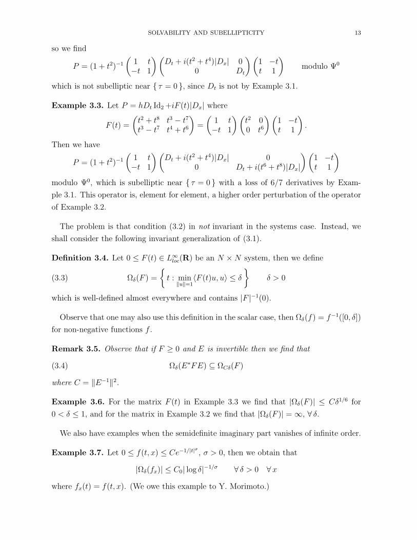
SOLVABILITY AND SUBELLIPTICITY 13
so we find
P = (1 + t2)−1
(1 t−t 1
)(Dt + i(t2 + t4)|Dx| 0
0 Dt
)(1 −tt 1
)modulo Ψ0
which is not subelliptic near τ = 0 , since Dt is not by Example 3.1.
Example 3.3. Let P = hDt Id2+iF (t)|Dx| where
F (t) =
(t2 + t8 t3 − t7
t3 − t7 t4 + t6
)=
(1 t−t 1
)(t2 00 t6
)(1 −tt 1
).
Then we have
P = (1 + t2)−1
(1 t−t 1
)(Dt + i(t2 + t4)|Dx| 0
0 Dt + i(t6 + t8)|Dx|
)(1 −tt 1
)
modulo Ψ0, which is subelliptic near τ = 0 with a loss of 6/7 derivatives by Exam-
ple 3.1. This operator is, element for element, a higher order perturbation of the operator
of Example 3.2.
The problem is that condition (3.2) in not invariant in the systems case. Instead, we
shall consider the following invariant generalization of (3.1).
Definition 3.4. Let 0 ≤ F (t) ∈ L∞loc(R) be an N ×N system, then we define
(3.3) Ωδ(F ) =
t : min
‖u‖=1〈F (t)u, u〉 ≤ δ
δ > 0
which is well-defined almost everywhere and contains |F |−1(0).
Observe that one may also use this definition in the scalar case, then Ωδ(f) = f−1([0, δ])
for non-negative functions f .
Remark 3.5. Observe that if F ≥ 0 and E is invertible then we find that
(3.4) Ωδ(E∗FE) ⊆ ΩCδ(F )
where C = ‖E−1‖2.
Example 3.6. For the matrix F (t) in Example 3.3 we find that |Ωδ(F )| ≤ Cδ1/6 for
0 < δ ≤ 1, and for the matrix in Example 3.2 we find that |Ωδ(F )| = ∞, ∀ δ.
We also have examples when the semidefinite imaginary part vanishes of infinite order.
Example 3.7. Let 0 ≤ f(t, x) ≤ Ce−1/|t|σ , σ > 0, then we obtain that
|Ωδ(fx)| ≤ C0| log δ|−1/σ ∀ δ > 0 ∀ x
where fx(t) = f(t, x). (We owe this example to Y. Morimoto.)

14 NILS DENCKER
We shall study systems where the imaginary part F vanishes of finite order, so that
|Ωδ(F )| ≤ Cδµ for µ > 0. In general, the largest exponent could be any µ > 0, for example
when F (t) = |t|1/µ IdN . But for C∞ systems the best exponent is µ = 1/k for an even k,
by the following result, which is Proposition A.2 in [3].
Remark 3.8. Assume that 0 ≤ F (t) ∈ C∞(R) is an N×N system such that F (t) ≥ c > 0
when |t| ≫ 1. Then we find that
|Ωδ(F )| ≤ Cδµ 0 < δ ≤ 1
if and only if µ ≤ 1/k for an even k ≥ 0 so that
(3.5)∑
j≤k
|∂jt 〈F (t)u(t), u(t)〉|/‖u(t)‖2 > 0 ∀ t
for any 0 6= u(t) ∈ C∞(R).
Example 3.9. For the scalar symbols τ + if(t, x, ξ) in Example 3.1 we find from Re-
mark 3.8 that (3.1) is equivalent to
| t : f(t, x, ξ) ≤ δ | = |Ωδ(fx,ξ)| ≤ Cδ1/k 0 < δ ≤ 1 |ξ| = 1
where fx,ξ(t) = f(t, x, ξ).
The following example shows that for subelliptic type of estimates it is not sufficient
to have conditions only on the vanishing of the symbol, we also need conditions on the
semibicharacteristics of the eigenvalues.
Example 3.10. Let
P = Dt Id2 +α
(Dx 00 −Dx
)+ i(t− βx)2|Dx| Id2 (t, x) ∈ R2
with α, β ∈ R, then we see from the scalar case in Example 3.1 that P is subelliptic near
τ = 0 with a loss of 2/3 derivatives if and only either α = 0 or α 6= 0 and β 6= ±1/α.
Definition 3.11. Let Q ∈ C∞(T ∗X) be an N ×N system and let w0 ∈ Σ ⊂ T ∗X , then
Q satisfies the approximation property on Σ near w0 if there exists a Q invariant C∞
subbundle V of CN over T ∗X such that V(w0) = KerQN (w0) and
(3.6) Re〈Q(w)v, v〉 = 0 v ∈ V(w) w ∈ Σ
near w0. That V is Q invariant means that Q(w)v ∈ V(w) for v ∈ V(w).
Here KerQN (w0) is the space of the generalized eigenvectors corresponding to the
zero eigenvalue. The symbol of the system in Example 3.10 satisfies the approximation
property on Σ = τ = 0 if and only if α = 0.

SOLVABILITY AND SUBELLIPTICITY 15
Let Q = Q∣∣Vthen Im iQ = Re Q = 0 so Lemma 2.13 gives that Ran Q⊥Ker Q on Σ.
Thus Ker QN = Ker Q on Σ, and since Ker QN (w0) = V(w0) we find that KerQN (w0) =
V(w0) = KerQ(w0).
Remark 3.12. Assume that Q satisfies the approximation property on the C∞ hypersur-
face Σ and is quasi-symmetric with respect to V /∈ TΣ. Then the limits of the non-trivial
semibicharacteristics of the eigenvalues of Q close to zero coincide with the bicharacter-
istics of Σ.
In fact, the approximation property in Definition 3.11 gives that 〈ReQu, u〉 = 0 for
u ∈ KerQ when τ = 0. Since ImQ ≥ 0 we find that
(3.7) 〈dQu, u〉 = 0 ∀ u ∈ KerQ on TΣ
By Remark 2.19 the limits of the non-trivial semibicharacteristics of the eigenvalues close
to zero of Q are curves with tangents determined by 〈dQu, u〉 for u ∈ KerQ. Since
V ReQ 6= 0 on KerQ we find from (3.7) that the limit curves coincide with the bicharac-
teristics of Σ, which are the flow-outs of the Hamilton vector field.
Example 3.13. Observe that Definition 3.11 is empty if DimKerQN (w0) = 0. If
DimKerQN(w0) > 0, then there exists ε > 0 and a neigborhood ω to w0 so that
(3.8) Π(w) =1
2πi
∫
|z|=ε
(z IdN −Q(w))−1 dz ∈ C∞(ω)
is the spectral projection on the (generalized) eigenvectors with eigenvalues having abso-
lute value less than ε. Then RanΠ is a Q invariant bundle over ω so that RanΠ(w0) =
KerQN (w0). Condition (3.6) with V = RanΠ means that Π∗ReQΠ ≡ 0 in ω. When
ImQ(w0) ≥ 0 we find that Π∗QΠ(w0) = 0, then Q satisfies the approximation property
on Σ near w0 with V = RanΠ if and only if
d(Π∗(ReQ)Π)∣∣TΣ
≡ 0 near w0
Example 3.14. If Q satisfies the approximation property on Σ, then by choosing an
orthonormal basis for V and extending it to an orthonormal basis for CN we obtain the
system on the form
Q =
(Q11 Q12
0 Q22
)
where Q11 is K ×K system such that QN11(w0) = 0, ReQ11 = 0 on Σ and |Q22| 6= 0. By
multiplying from left with (IdK −Q12Q
−122
0 IdN−K
)
we obtain that Q12 ≡ 0 without changing Q11 or Q22.

16 NILS DENCKER
In fact, the eigenvalues of Q are then eigenvalues of either Q11 or Q22. Since V(w0) are
the (generalized) eigenvectors corresponding to the zero eigenvalue of Q(w0) we find that
all eigenvalues of Q22(w0) are non-vanishing, thus Q22 is invertible near w0,
Remark 3.15. If Q satisfies the approximation property on Σ near w0, then it satisfies
the approximation property on Σ near w1, for w1 sufficiently close to w0.
In fact, let Q11 be the restriction of Q to V as in Example 3.14, then since ReQ11 =
Im iQ11 = 0 on Σ we find from Lemma 2.13 that RanQ11⊥KerQ11 and KerQ11 = KerQN11
on Σ. Since Q22 is invertible in (3.14), we find that KerQ ⊆ V. Thus, by using the spectral
projection (3.8) of Q11 near w1 ∈ Σ for small enough ε we obtain an Q invariant subbundle
V ⊆ V so that V(w1) = KerQ11(w1) = KerQN(w1).
If Q ∈ C∞ satisfies the approximation property and QE = E∗QE with invertible
E ∈ C∞, then it follows from the proof of Proposition 3.20 below that there exist invertible
A, B ∈ C∞ so that AQE and Q∗B satisfy the approximation property.
Definition 3.16. Let P (w) ∈ C∞(T ∗X) be an N ×N system and µ ∈ R+. Then P is of
finite type µ at w0 ∈ T ∗X if there exists a neighborhood ω of w0, a C∞ hypersurface Σ ∋
w0, a real C∞ vector field V /∈ TΣ and an invertible symmetrizer M ∈ C∞ so that
Q = MP is quasi-symmetric with respect to V in ω and satisfies the approximation
property on Σ⋂ω. Also, for every bicharacteristic γ of Σ the arc length
(3.9)∣∣γ ∩ Ωδ(ImQ) ∩ ω
∣∣ ≤ Cδµ 0 < δ ≤ 1
The operator P ∈ Ψmcl is of finite type µ at w0 if the principal symbol σ(P ) is of finite
type when |ξ| = 1.
Recall that the bicharacteristics of a hypersurface in T ∗X are the flow-outs of the
Hamilton vector field of Σ. Of course, if P is elliptic then it is trivially of finite type
0, just choose M = iP−1 to obtain Q = i IdN . If P is of finite type, then it is quasi-
symmetrizable by definition and thus of principal type.
Remark 3.17. Observe that since 0 ≤ ImQ ∈ C∞ we obtain from Remark 3.8 that the
largest exponent in (3.9) is µ = 1/k for an even k ≥ 0. Also, we may assume that
(3.10) Im〈Qu, u〉 ≥ c‖Qu‖2 ∀ u ∈ CN
In fact, by adding iP ∗ to M we obtain (3.10) for large enough by (2.7), and this
does not change ReQ.
Example 3.18. Assume that Q is quasi-symmetric with respect to the real vector field V ,
satisfying (3.9) and the approximation property on Σ. Then by choosing an orthonormal

SOLVABILITY AND SUBELLIPTICITY 17
basis and changing the symmetrizer as in Example 3.14 we obtain the system on the form
Q =
(Q11 00 Q22
)
where Q11 is K×K system such that QN11(w0) = 0, ReQ11 = 0 on Σ and |Q22| 6= 0. Since
Q is quasi-symmetric with respect to V we also obtain that Q11(w0) = 0, ReV Q11 > 0,
ImQ ≥ 0 and Q satisfies (3.9). In fact, then we find from Lemma 2.13 that ImQ⊥KerQ
which gives KerQN = KerQ. Note that Ωδ(ImQ11) ⊆ Ωδ(ImQ), so Q11 satisfies (3.9).
Example 3.19. In the scalar case, we find from Example 2.9 that p ∈ C∞(T ∗X) is
quasi-symmetrizable with respect to Ht = ∂τ if and only if
(3.11) p(t, x; τ, ξ) = q(t, x; τ, ξ)(τ + if(t, x, ξ))
with f ≥ 0 and q 6= 0. If f(t, x, ξ) ≥ c > 0 when |(t, x, ξ)| ≫ 1 we find by taking q−1 as
symmetrizer that p is of finite type µ if and only if µ = 1/k for an even k such that∑
j≤k
|∂kt f(t, x, ξ)| > 0 ∀ x ξ
by Remark 3.8. In fact, the approximation property on Σ = τ = 0 is trivial since f is
real.
Proposition 3.20. If P (w) ∈ C∞(T ∗X) is of finite type µ at w then P ∗ is of finite type
µ at w. If A(w) and B(w) ∈ C∞(T ∗X) are invertible, then APB is of finite type µ at w.
Proof. Let M be the symmetrizer in Definition 3.16 so that Q =MP is quasi-symmetric
with respect to V . By choosing a suitable basis and changing the symmetrizer as in
Example 3.18, we may write
(3.12) Q =
(Q11 00 Q22
)
where Q11 is K × K system such that Q11(w0) = 0, V ReQ11 > 0, ReQ11 = 0 on
Σ and Q22 is invertible. We also have ImQ ≥ 0 and Q satisfies (3.9). Let V1 =u ∈ CN : uj = 0 for j > K
and V2 =
u ∈ CN : uj = 0 for j ≤ K
, these are Q in-
variant bundles such that V1 ⊕ V2 = CN .
First we are going to show that P = APB is of finite type. By taking M = B−1MA−1
we find that
(3.13) MP = Q = B−1QB
and it is clear that B−1Vj are Q invariant bundles, j = 1, 2. By choosing bases in B−1Vj
for j = 1, 2, we obtain a basis for CN in which Q has a block form:
(3.14) Q =
(Q11 0
0 Q22
)
18 NILS DENCKER
Here Qjj : B−1Vj 7→ B−1Vj, is given by Qjj = B−1
j QjjBj with
Bj : B−1Vj ∋ u 7→ Bu ∈ Vj j = 1, 2
By multiplying Q from the left with
B =
(B∗
1B1 00 B∗
2B2
)
we obtain that
Q = BQ = BMP =
(B∗
1Q11B1 00 B∗
2Q22B2
)=
(Q11 00 Q22
)
It is clear that ImQ ≥ 0, Q11(w0) = 0, ReQ11 = 0 on Σ, |Q22| 6= 0 and V ReQ11 > 0 by
Proposition 2.14. Finally, we obtain from Remark 3.5 that
(3.15) Ωδ(ImQ) ⊆ ΩCδ(ImQ)
for some C > 0, which proves that P = APB is of finite type. Observe that Q = AQB,
where QB = B∗QB and A = BB−1(B∗)−1.
To show that P ∗ also is of finite type, we may assume as before that Q =MP is on the
form (3.12) with Q11(w0) = 0, V ReQ11 > 0, ReQ11 = 0 on Σ, Q22 is invertible, ImQ ≥ 0
and Q satisfies (3.9). Then we find that
−P ∗M∗ = −Q∗ =
(−Q∗
11 00 −Q∗
22
)
satisfies the same conditions with respect to −V , so it is of finite type with multiplier IdN .
By the first part of the proof we obtain that P ∗ is of finite type, which finishes the
proof.
Theorem 3.21. Assume that P ∈ Ψmcl (X) is an N × N system of finite type µ > 0
near w0 ∈ T ∗X \ 0, then P is subelliptic at w0 with a loss of 1/µ+ 1 derivatives:
(3.16) Pu ∈ H(s) at w0 =⇒ u ∈ H(s+m−1/µ+1) at w0
for u ∈ D′(X,CN).
Observe that the largest exponent is µ = 1/k for an even k by Remark 3.17, and
then 1/µ + 1 = k/k + 1. Thus Theorem 3.21 generalizes Proposition 27.3.1 in [5] by
Example 3.19.
Example 3.22. Let
P (t, x; τ, ξ) = τM(t, x, ξ) + iF (t, x, ξ) ∈ S1cl
where M ≥ c0 > 0 and F ≥ 0 satisfies
(3.17)
∣∣∣∣t : inf
|u|=1〈F (t, x, ξ)u, u〉 ≤ δ
∣∣∣∣ ≤ Cδµ |ξ| = 1
SOLVABILITY AND SUBELLIPTICITY 19
for some µ > 0. Then P is quasi-symmetrizable with respect to ∂τ with symmetrizer IdN .
When τ = 0 we obtain that ReP = 0, so by taking V = RanΠ for the spectral projection
Π given by (3.8) for F , we find that P satisfies the approximation property with respect
to Σ = τ = 0 . Since Ωδ(ImP ) = Ωδ(F ) we find from (3.17) that P is of finite type µ.
Observe that if F (t, x, ξ) ≥ c > 0 when |(t, x, ξ)| ≫ 1 we find from Remark 3.8 that (3.17)
is satisfied if and only if µ ≤ 1/k for an even k ≥ 0 so that∑
j≤k
|∂jt 〈F (t, x, ξ)u(t), u(t)〉| > 0 ∀ t, x, ξ
for any 0 6= u(t) ∈ C∞(R). Theorem 3.21 gives that P (t, x,Dt, Dx) is subelliptic
near τ = 0 with a loss of k/k + 1 derivatives.
Proof of Theorem 3.21. First, we may reduce to the case m = s = 0 by replacing u and P
by 〈D〉s+mu and 〈D〉sP 〈D〉−s−m ∈ Ψ0cl. Now u ∈ H(−K) for some K near w0, and it is no
restriction to assume K = 1. In fact, if K > 1 then by using that Pu ∈ H(1−K) near w0,
we obtain that u ∈ H(−K+µ/µ+1) near w0 and we may iterate this argument until u ∈ H(−1)
near w0. By cutting off with φ ∈ S01,0 we may assume that v = φ(x,D)u ∈ H(−1) and
Pv = [P, φ(x,D)]u + φ(x,D)Pu ∈ H(0) since [P, φ(x,D)] ∈ Ψ−1. If φ 6= 0 in a conical
neighborhood of w0 it suffices to prove that v ∈ H(−1/µ+1).
By Definition 3.16 and Remark 3.17 there exist a C∞ hypersurface Σ, a real C∞ vector
field V /∈ TΣ, an invertible symmetrizer M ∈ C∞ so that Q = MP satisfies (3.9), the
approximation property on Σ, and
V ReQ ≥ c− C ImQ c > 0(3.18)
ImQ ≥ cQ∗Q(3.19)
in a neighborhood ω of w0. By extending by homogeneity, we can assume that V , M
and Q are homogeneous of degree 0.
Since (3.18) is stable under small perturbations in V we can replace V with Ht for some
real t ∈ C∞. By solving the initial value problem Htτ ≡ −1, τ∣∣Σ= 0, and completing
to a symplectic C∞ coordinate system (t, τ, x, ξ), we obtain that Σ = τ = 0 in a
neighborhood of w0 = (0, 0, x0, ξ0), ξ0 6= 0. We obtain from Definition 3.11 that
(3.20) Re〈Qu, u〉 = 0 when u ∈ V and τ = 0
near w0. Here V is a Q invariant C∞ subbundle of CN such that V(w0) = KerQN(w0) =
KerQ(w0) by Lemma 2.13. By condition (3.9) we have that
(3.21)∣∣Ωδ(ImQx,ξ) ∩ |t| < c
∣∣ ≤ Cδµ
when |(x, ξ)− (x0, ξ0)| < c, here Qx,ξ(t) = Q(t, 0, x, ξ).

20 NILS DENCKER
Next, we shall localize the estimate. Choose ϕj j ∈ S01,0 and ψj j ∈ S0
1,0 with
values in ℓ2, such that ϕj ≥ 0, ψj ≥ 0,∑
j ϕ2j = 1, ψjϕj ≡ ϕj and ψj is supported where
|(τ, ξ)| ∼= 2j. Since these are Fourier multipliers we find that∑
j ϕj(Dt,x)2 = 1 and
‖u‖2(s) ∼=∑
j
22sj‖ϕj(Dt,x)u‖2 u ∈ S
Let Qj = ψjQ be the localized symbol, and let hj = 2−j ≤ 1. Since Qj ∈ S01,0 is
supported where |(τ, ξ)| ∼= 2j , we find that Qj(t, x, τ, ξ) = Qj(t, x, hjτ, hjξ) where Qj ∈C∞
0 (T ∗Rn) uniformly. We shall obtain Theorem 3.21 from the following result, which is
Proposition 6.1 in [3].
Proposition 3.23. Assume that Q ∈ C∞b (T ∗Rn) is an N ×N system satisfying (3.18)–
(3.21) in a neighborhood of w0 = (0, 0, x0, ξ0) with V = ∂τ and µ > 0. Then there
exists h0 > 0 and R ∈ C∞b (T ∗Rn) so that w0 /∈ suppR and
(3.22) h1/µ+1‖u‖ ≤ C(‖Q(t, x, hDt,x)u‖+ ‖Rw(t, x, hDt,x)u‖+ h‖u‖) 0 < h ≤ h0
for any u ∈ C∞0 (Rn,CN).
Here C∞b are C∞ functions with L∞ bounds on any derivative, and the result is uniform
in the usual sense. Observe that this estimate can be extended to a semiglobal estimate.
In fact, let ω be a neighborhood of w0 such that suppR⋂ω = ∅, where R is given by
Proposition 3.23. Take ϕ ∈ C∞0 (ω) such that 0 ≤ ϕ ≤ 1 and ϕ = 1 in a neighborhood
of w0. By substituting ϕ(t, x, hDt,x)u in (3.22) we obtain from the calculus
(3.23)
h1/µ+1‖ϕ(t, x, hDt,x)u‖ ≤ CN(‖ϕ(t, x, hDt,x)Q(t, x, hDt,x)u‖+ h‖u‖) ∀ u ∈ C∞0
for small enough h since Rϕ ≡ 0 and ‖[Q(t, x, hDt,x), ϕ(t, x, hDt,x)]u‖ ≤ Ch‖u‖. Thus,
if Q satisfies conditions (3.18)–(3.21) near any w ∈ K ⋐ T ∗Rn, then by using Bolzano-
Weierstrass we obtain the estimate (3.22) with suppR⋂K = ∅.
Now, by using that Qj satisfies (3.18)–(3.21) in a neighborhood of suppϕj, we obtain
the estimate (3.22) for Qj(t, x, hDt,x) with h = hj = 2−j ≪ 1 and R = Rj ∈ S01,0 such
that suppϕj
⋂suppRj = ∅. Substituting ϕj(Dt,x)u we obtain for j ≫ 1 that
2−j/µ+1‖ϕj(Dt,x)u‖ ≤ CN(‖Qj(t, x,Dt,x)ϕj(Dt,x)u‖+ ‖Rju‖+ 2−j‖ϕj(Dt,x)u‖) ∀ u ∈ S ′
where Rj = Rj(t, x,Dt,x)ϕj(Dt,x) ∈ Ψ−N with values in ℓ2. Now since Qj and Q are
uniformly bounded in S01,0 the calculus gives that
Qj(t, x,Dt,x)ϕj(Dt,x) = ϕj(Dt,x)Q(t, x,Dt,x) + j(t, x,Dt,x)

SOLVABILITY AND SUBELLIPTICITY 21
where j j ∈ Ψ−1 with values in ℓ2. Thus, by squaring and summing up, we obtain by
continuity that
(3.24) ‖u‖2(−1/µ+1) ≤ C(‖Q(t, x,Dt,x)u‖2 + ‖u‖2(−1)) u ∈ H(−1)
Since Q(t, x,Dt,x) = M(t, x,Dt,x)P (t, x,Dt,x) modulo Ψ−1 where M ∈ Ψ0, the calculus
gives
(3.25) ‖Q(t, x,Dt,x)u‖ ≤ C(‖M(t, x,Dt,x)P (t, x,Dt,x)u‖+ ‖u‖(−1))
≤ C ′(‖P (t, x,Dt,x)u‖+ ‖u‖(−1)) u ∈ H(−1)
which together with (3.24) proves Theorem 3.21.
References
1. N. Dencker, J. Sjostrand, and M. Zworski, Pseudospectra of semiclassical (pseudo-) differential oper-ators, Comm. Pure Appl. Math. 57 (2004), no. 3, 384–415.
2. N. Dencker, The resolution of the Nirenberg-Treves conjecture, Ann. of Math. 163 (2006), 405–444.3. , The pseudospectrum of systems of semiclassical operators, arXiv:0705.4561[math.AP]. To
appear in Analysis & PDE.4. , On the solvability of systems of pseudodifferential operators, arXiv:0801.4043[math.AP]. To
appear in Geometric Aspects of Analysis and Mechanics, A Conference in Honor of Hans Duistermaat.5. L. Hormander, The analysis of linear partial differential operators, vol. I–IV, Springer-Verlag, Berlin,
1983–1985.6. H. Lewy An example of a smooth linear partial differential equation without solution, Ann. of Math.
66 (1957), 155–158.7. L. Nirenberg and F. Treves, On local solvability of linear partial differential equations. Part I: Neces-
sary conditions, Comm. Partial Differential Equations 23 (1970), 1–38, Part II: Sufficient conditions,Comm. Pure Appl. Math. 23 (1970), 459–509; Correction, Comm. Pure Appl. Math. 24 (1971),279–288.
8. M. Taylor, Pseudodifferential operators, Princeton University Press, Princeton, N.J., 1981.
Centre for Mathematical Sciences, Lund University, Box 118, SE-221 00 Lund, Sweden
E-mail address : [email protected]


