Deconvolution, Deblurring andRestoration
T-61.182, Biomedical Image Analysis
Seminar Presentation 14.4.2005
Seppo Mattila & Mika Pollari
Overview (1/2)
• Linear space-invariant (LSI) restoration filters - Inverse filtering - Power spectrum equalization - Wiener filter - Constrained least-squares restoration - Metz filter• Blind Deblurring
Overview (2/2)
• Homomorphic Deconvolution• Space-variant restoration
– Sectioned image restoration– Adaptive-neighbourhood deblurring– The Kalman filter
• Applications - Medical - Astronomical
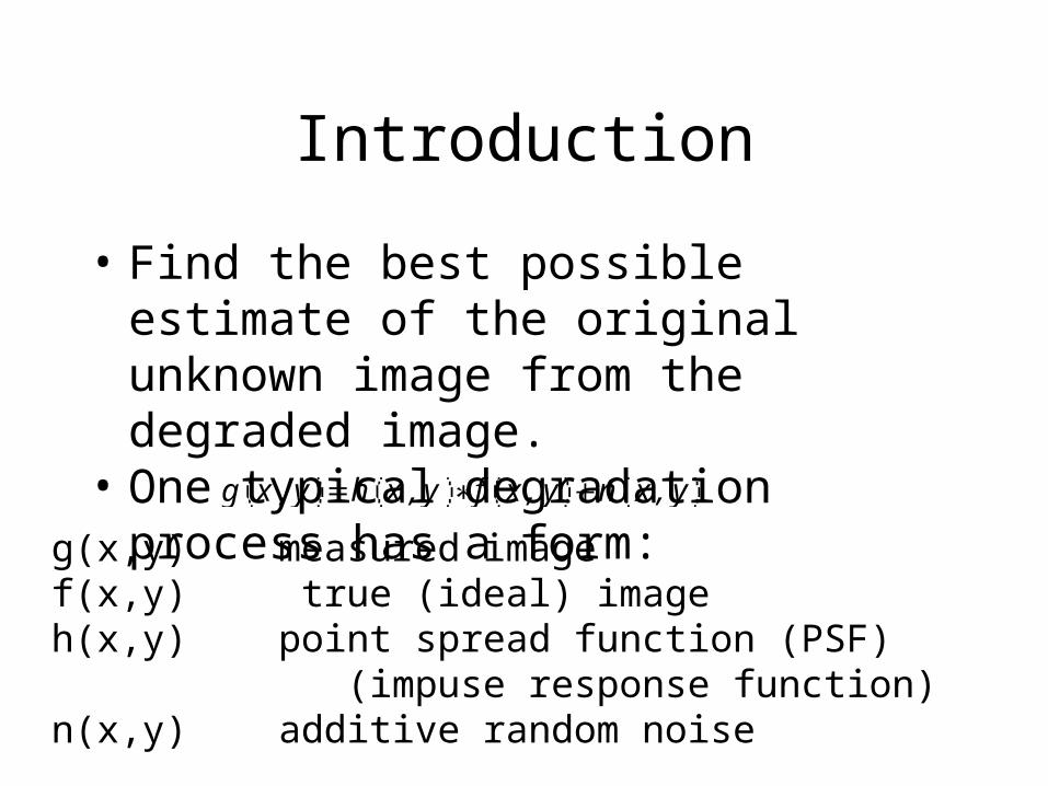
Introduction
• Find the best possible estimate of the original unknown image from the degraded image.
• One typical degradation process has a form:g x ,y h x ,y f x , y n x, y
g(x,y) measured imagef(x,y) true (ideal) imageh(x,y) point spread function (PSF) (impuse response function)n(x,y) additive random noise
Image Restoration General
• One has to have some a priori knowledge about the degragation process.
• Usually one needs 1) model for degragation, some information from 2) original image and 3) noise.
• Note! Eventhough one doesn’t know the original image some information such as power spectral density (PSD) and autocorreletion function (ACF) are easy to model.
Linear-Space Invariant (LSI) Restoration Filters
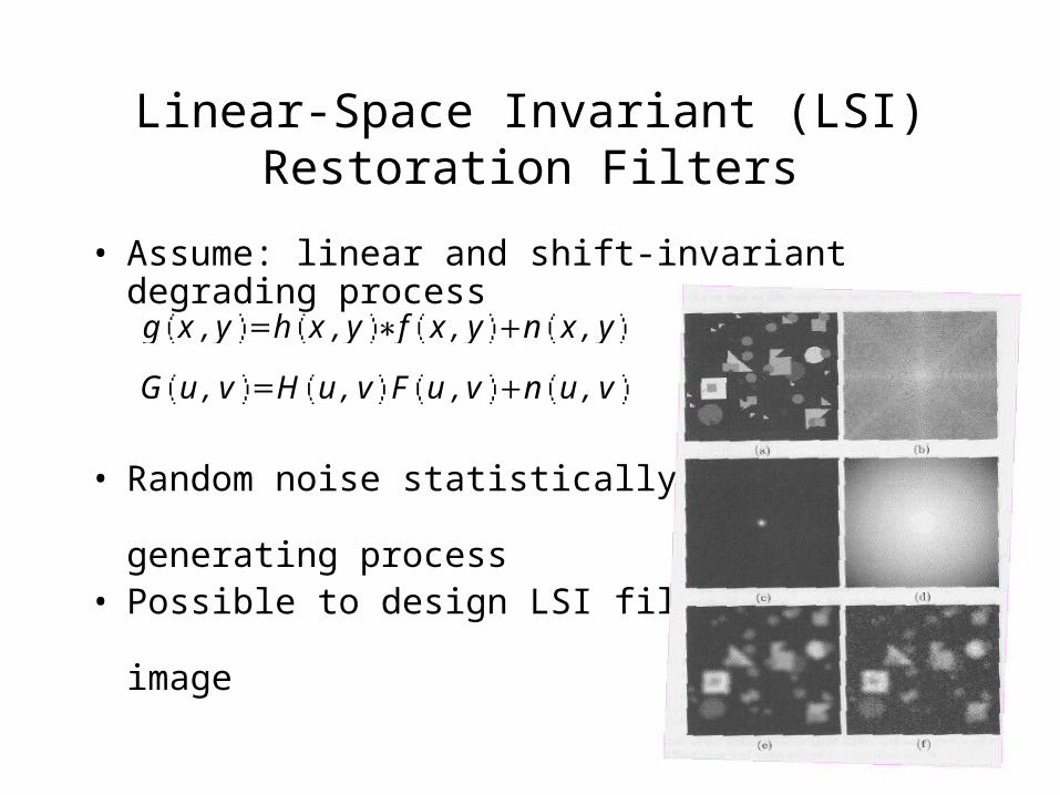
• Assume: linear and shift-invariant degrading process
• Random noise statistically indep. of image-generating process
• Possible to design LSI filters to restore the image
g x ,y h x ,y f x , y n x, y
G u, v H u, v F u ,v n u, v

Inverse Filtering
• Consider degrading process in matrix form:
• Given g and h, estimate f by minimising the squared error between observed image (g) and :
where and are approximations of f and g
• Set derivative of є2 to zero:
2 T gTg f ThTg gThf f ThThf
g hf
g g g h f
F u,vG u,vH u, v
(see Sect. 3.5.3 for details)
F u,vG u,vH u, v
n u,vH u, v
(if no noise)
(if noise present)
f g
g
Inverse Filtering Examples
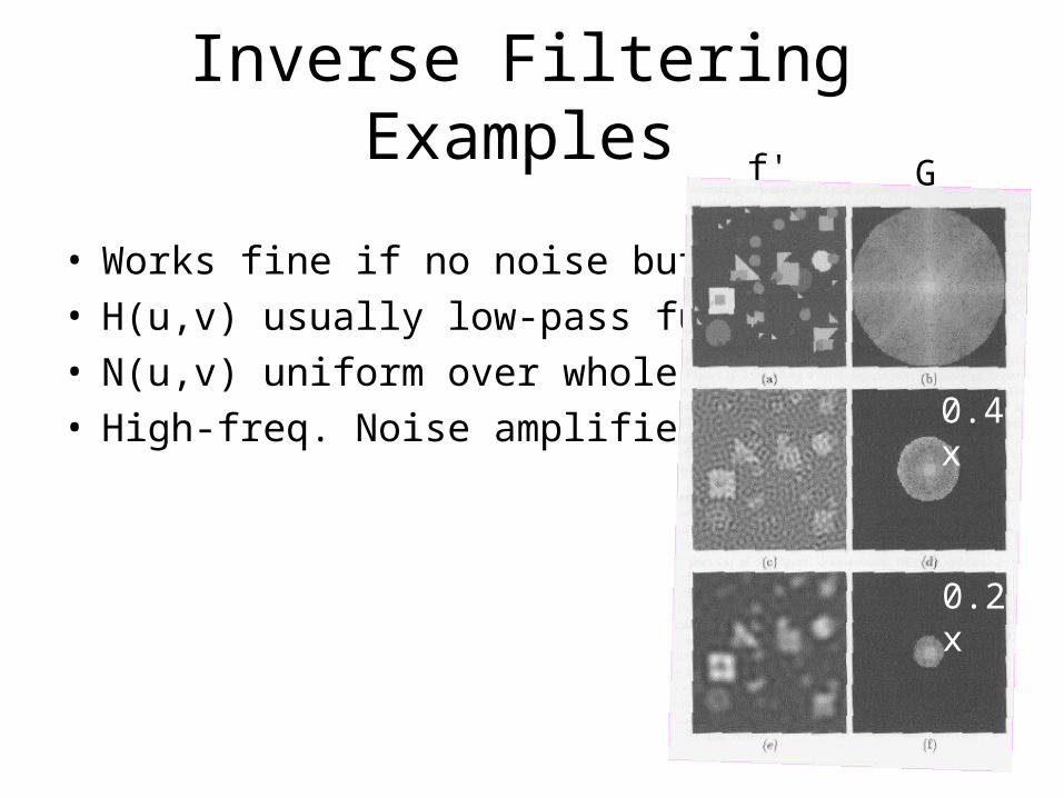
• Works fine if no noise but...
• H(u,v) usually low-pass function.
• N(u,v) uniform over whole spectrum.
• High-freq. Noise amplified!! 0.4x
0.2x
f' G
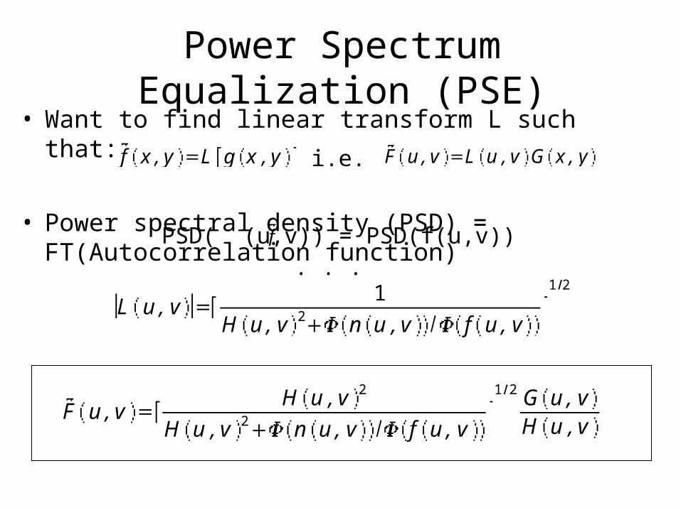
Power Spectrum Equalization (PSE)• Want to find linear transform L such that:
• Power spectral density (PSD) = FT(Autocorrelation function)
f x ,y L g x ,y
PSD( (u,v)) = PSD(f(u,v))
L u, v1
H u, v 2 n u ,v f u, v
1 2
F u,vH u ,v 2
H u ,v 2 n u, v f u, v
1 2G u, vH u ,v
i.e. F u,v L u ,v G x, y
f
. . .
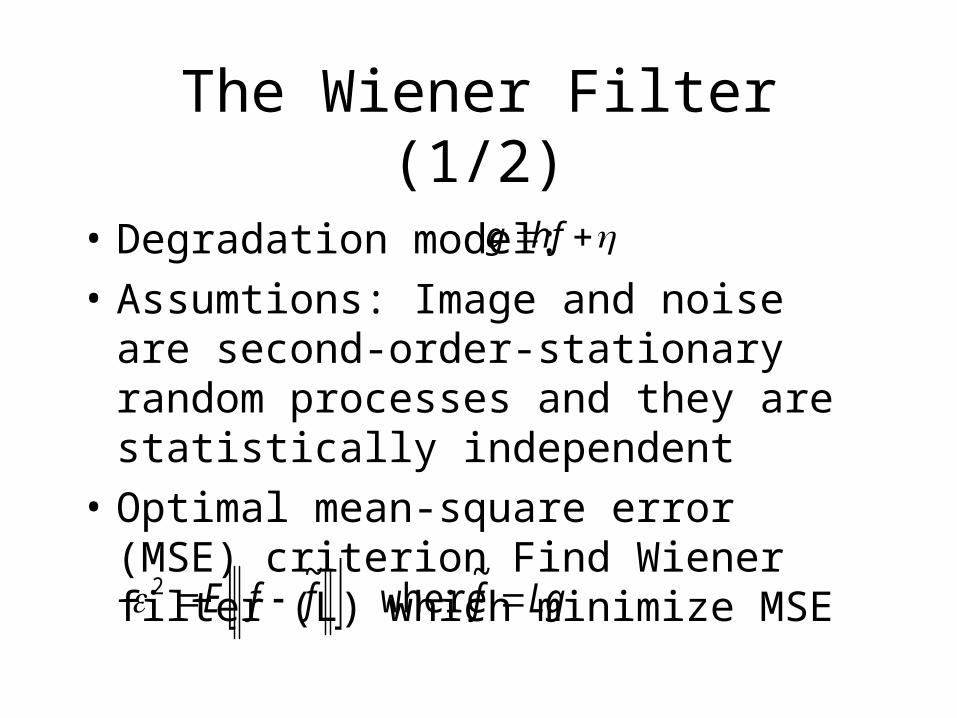
The Wiener Filter (1/2)
• Degradation model:
• Assumtions: Image and noise are second-order-stationary random processes and they are statistically independent
• Optimal mean-square error (MSE) criterion Find Wiener filter (L) which minimize MSE
hfg
LgfffE ~
where~2

The Wiener Filter (2/2)
• Minimizing the criterion we end up to optimal Wiener filter.
• The Wiener filter depends on the autocorrelation function (ACF) of the image and noise (This is no problem).
• In general ACFs are easy to estimate.
1)( Tf
Tfw hhhL
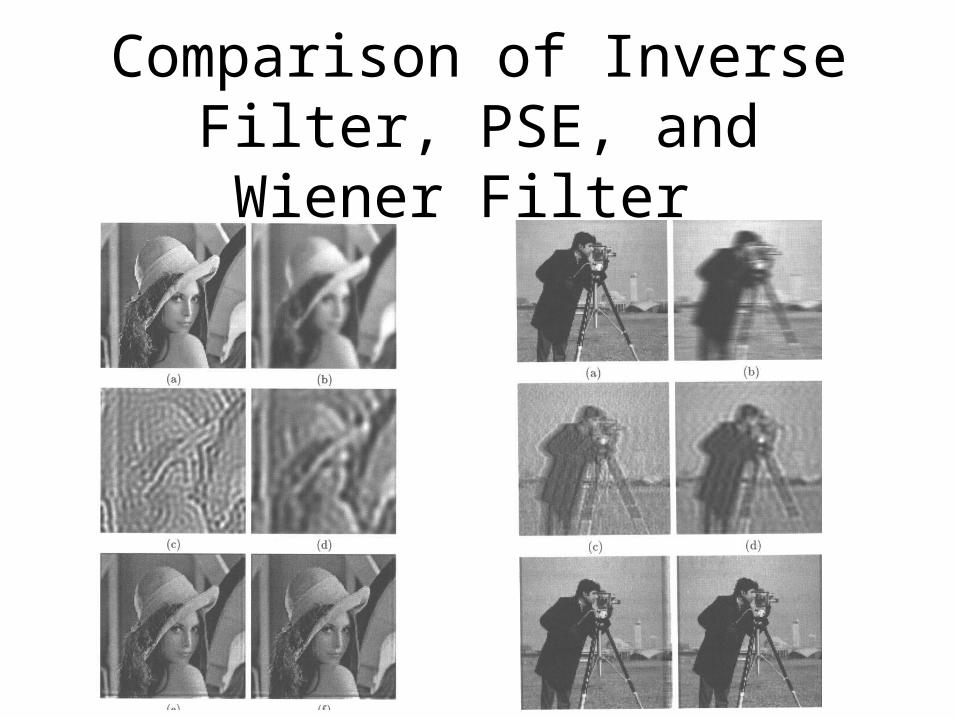
Comparison of Inverse Filter, PSE, and Wiener Filter

Constrained Least-squares Restoration
• Minimise: with constraint: where L is a linear filter operator
● Similar to Wiener filter but does not require the PSDs of the image and noise to be known
● The mean and variance of the noise needed to set optimally. If = 0 inverse filter
Lf2
g h f2
n 2
F u,vH u, v 2
H u, v 2 L u, v 2
G u, vH u,v
. . .

The Metz Filter
• Modification to inverse filter.
• Supress the high frequency noise instead of amplyfying it.
• Select factor so that mean-square error (MSE) between ideal and filtered image is minimized.
),(
),(11 2
vuH
vuHLM
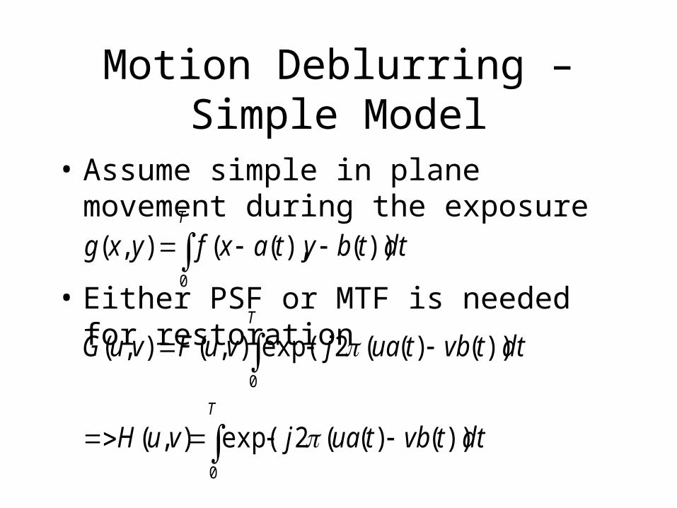
Motion Deblurring – Simple Model
• Assume simple in plane movement during the exposure
• Either PSF or MTF is needed for restoration T
dttbytaxfyxg0
))(),((),(
T
T
dttvbtuajvuH
dttvbtuajvuFvuG
0
0
))()((2exp(),(
))()((2exp(),(),(

Blind Deblurring
• Definition of deblurring.
• Blind deblurring: models of PSF and noise are not known – cannot be estimated separately.
• Degragated image (in spectral domain) consist some information of PSF and noise but in combined form.
),(),(),( yxyxfPSFyxg

Method 1 – Extension to PSE
• Broke image to M x M size segment where M is larger than dimensions of PSF then
• Average of PSD of these segments tend toward the true signal and noise PSD
• This is combined information of blur function and noise which is needed in PSE
• Finaly, only PSD of image is needed
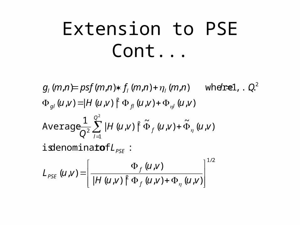
Extension to PSE Cont...
2/1
2
1
22
2
2
),(),(|),(|
),(),(
: ofr denominato is
),(~
),(~
|),(|1
:Average
),(),(|),(|),(
,...,1 where),(),(),(),(
2
vuvuvuH
vuvuL
L
vuvuvuHQ
vuvuvuHvu
Qlnmnmfnmpsfnmg
f
fPSE
PSE
Q
lf
lflgl
lll

Method 2 – Iterative Blind Deblurring
• Assumptation: MTF of PSF has zero phase.
• Idea: blur function affects in PSD but phase information preserves original information from edges.
),(),( and v)(u,v)M(u,M ),(M
FT of mag./phase look the and zero tonoiseset
),(),(),(),(
fPSFg vuvuvu
yxyxfyxpsfyxg
fg
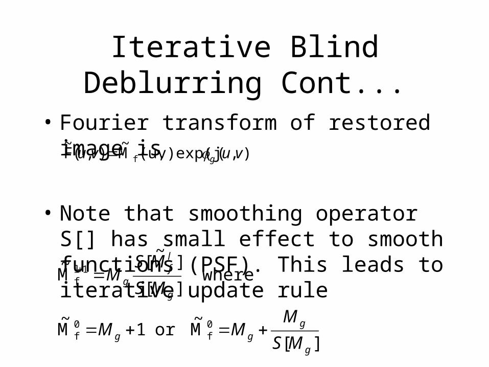
Iterative Blind Deblurring Cont...
• Fourier transform of restored image is
• Note that smoothing operator S[] has small effect to smooth functions (PSF). This leads to iterative update rule
)),(v)exp(j(u,M~
),(F~
f vuvu g
][ M
~or 1 M
~
where][
]~
[M~
0f
0f
1lf
g
ggg
g
lf
g
MS
MMM
MS
MSM

Examples of Iterative Blind Deblurring

Homomorphic deconvolution
• Start from:• Convert convolution operation to addition:
● Complex cepstrum:
Complex cepstra related: ● Practical application, however, not simple...
G u, v H u, v F u ,v
log G u,v log H u, v log F u, v
g x ,y FT 1 log G u, v
g x ,y h x ,y f x ,y
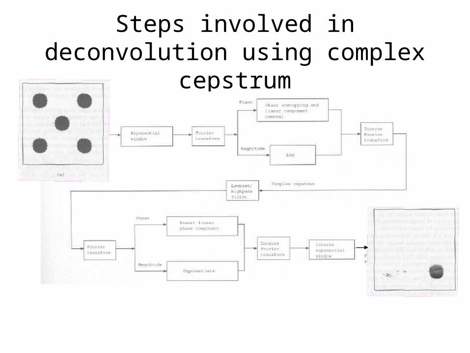
Steps involved in deconvolution using complex cepstrum

Space-variant Image Restoration
• So far we have assumed that images are spatially (and temporaly) stationary
• This is (generally) not true – at the best images are locally stationary
• Techniques to overcome this problem:– Sectioned image restoration– Adaptive neighbourhood deblurring– The Kalman filter (the most elegant approach)
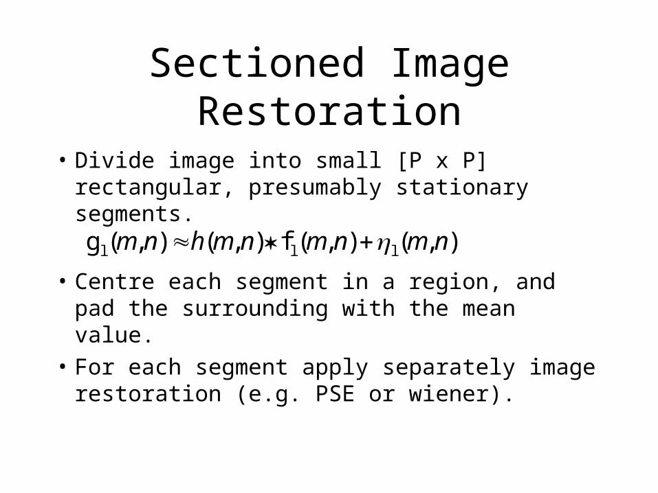
Sectioned Image Restoration
• Divide image into small [P x P] rectangular, presumably stationary segments.
• Centre each segment in a region, and pad the surrounding with the mean value.
• For each segment apply separately image restoration (e.g. PSE or wiener).
),(),(f),(),(g lll nmnmnmhnm
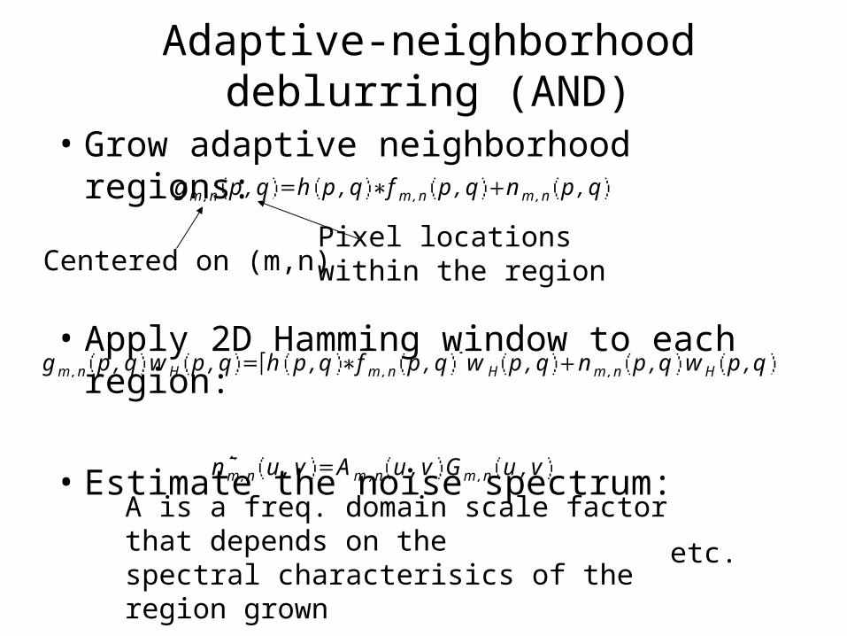
Adaptive-neighborhood deblurring (AND)
• Grow adaptive neighborhood regions:
• Apply 2D Hamming window to each region:
• Estimate the noise spectrum:
gm,n p,q h p,q fm,n p,q nm,n p,q
Centered on (m,n) Pixel locationswithin the region
gm,n p,q wH p,q h p,q fm,n p,q wH p,q nm,n p,q wH p,q
nm,n u, v Am,n u ,v Gm,n u ,v
A is a freq. domain scale factor that depends on the spectral characterisics of the region grown etc.
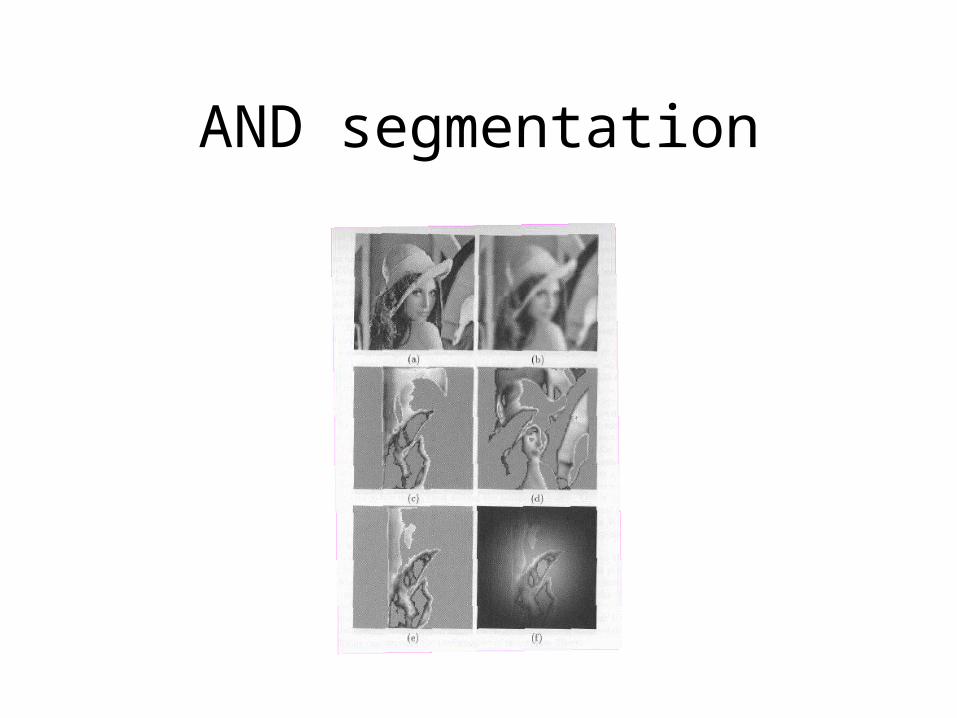
AND segmentation
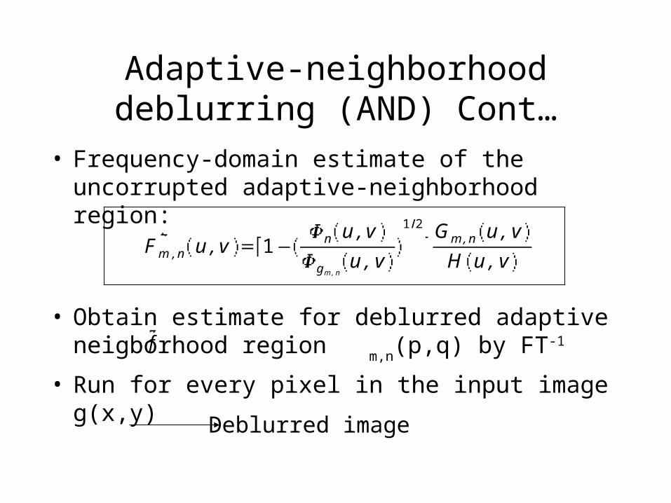
Adaptive-neighborhood deblurring (AND) Cont…
• Frequency-domain estimate of the uncorrupted adaptive-neighborhood region:
• Obtain estimate for deblurred adaptive neigborhood region
m,n(p,q) by FT-1
• Run for every pixel in the input image g(x,y)
Fm,n u,v 1 n u,v
gm,nu, v
1 2 Gm,n u, v
H u, v
Deblurred image
f
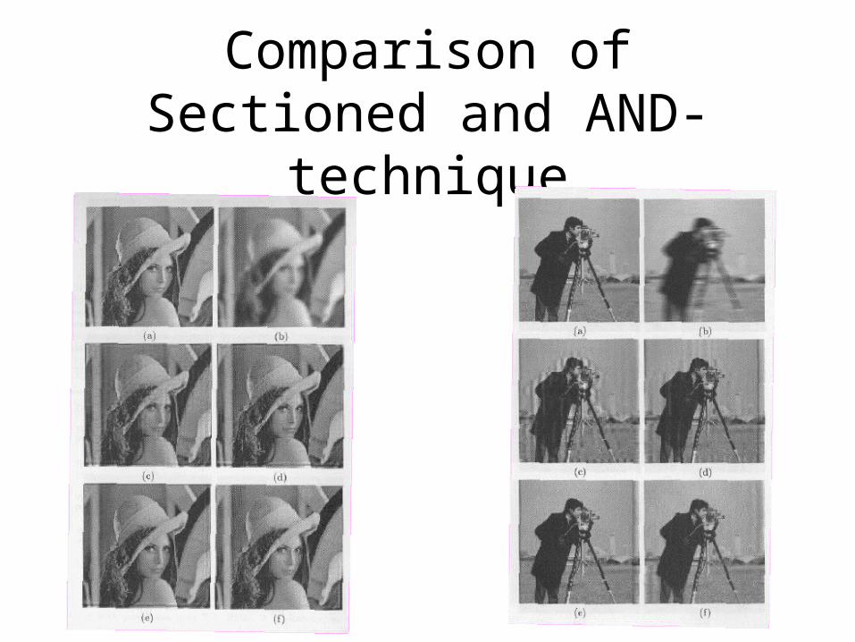
Comparison of Sectioned and AND-technique
Kalman Filter
• Kalman filter is a set of mathematical equations.
• Filter provides recursive way to estimate the state of the process (in non-stationary environment), so that mean of squared errors is minimized (MMSE).
• Kalman filter enables prediction, filtering, and smoothing.

Kalman Filter State-Space
• Process Eq.
• Observation Eq.
• Innovation process:
dn)f(n)1,a(n1)f(n
Oh(n)f(n)g(n)
)|(~)()( 1 nGngngn
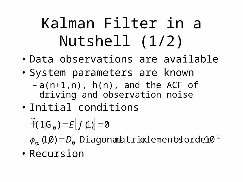
Kalman Filter in a Nutshell (1/2)
• Data observations are available • System parameters are known
– a(n+1,n), h(n), and the ACF of driving and observation noise
• Initial conditions
• Recursion
2
0
0
10order of elementsmatrix Diagonal )0,1(
0)1()G|(1f~
D
fE
p

Kalman Filter in a Nutshell (2/2)
1) Compute the Kalman gain K(n)
2) Obtain the innovation process
3) Update
4) Compute the ACF of filtered state error
5) Compute the ACF of predicted state error
10 )]()()1,()([)()1,(n)1,a(nK(n) nnhnnnhnhnn T
pT
p
)|(~
)()()( 1 nGnfnhngn
)()()|(~
),1()|1(~
1 nnKGnfnnaGnf nn
)1,()()()1,()1,()( nnnhnKnnannn ppp
)(),1()(),1(),1( nnnannnann ndT
pp

Wiener Filter Restoration of Digital Radiography
Astronomical applications
• Images blurred by atmospheric turbulence• Observing above the atmosphere very expensive (HST)• Improve the ground-based resolution by
– Suitable sites for the observatory (@ 4 km height)– Real time Adaptive optics correction– Deconvolution
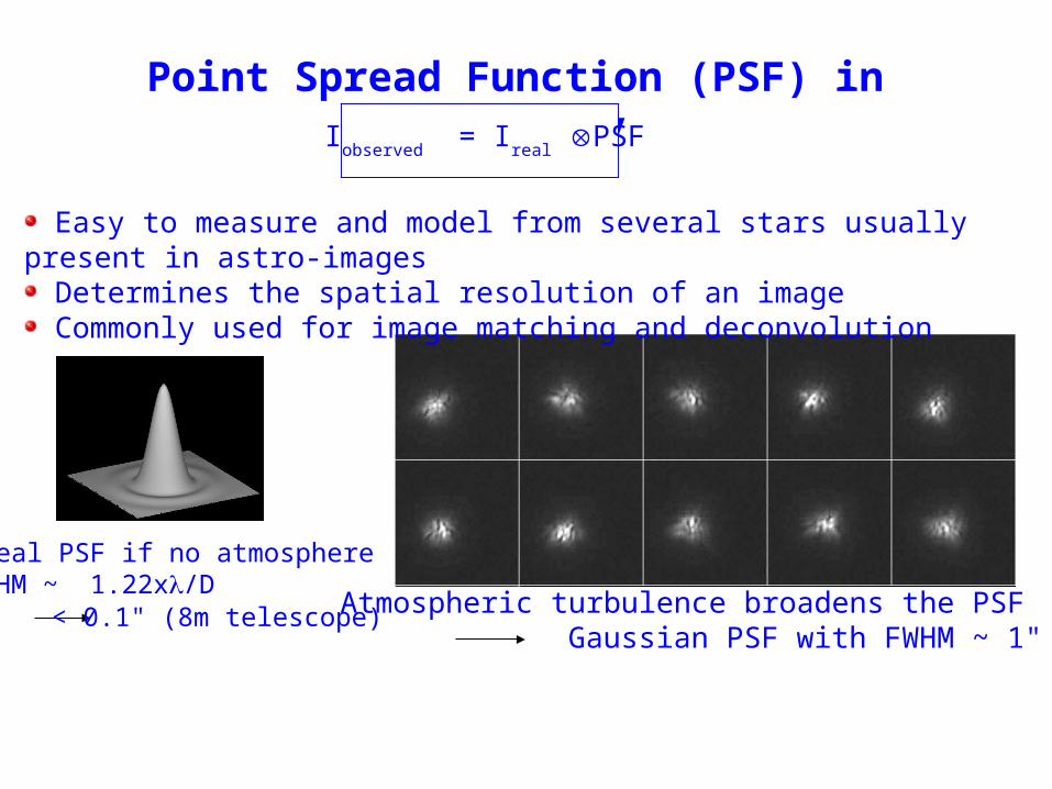
Point Spread Function (PSF) in Astronomy
Ideal PSF if no atmosphereFWHM ~ 1.22x/D
< 0.1" (8m telescope) Atmospheric turbulence broadens the PSF Gaussian PSF with FWHM ~ 1"
Iobserved
= Ireal
⊗PSF
Easy to measure and model from several stars usually present in astro-images Determines the spatial resolution of an image Commonly used for image matching and deconvolution

Richardson-Lucy deconvolution
• Used in both fields: astronomy & medical imaging• Start from Bayes's theorem, end up with:
• Takes into account statistical fluctuations in the signal, therefore can reconstruct noisy images!
• In astronomy the PSF is known accurately
• From an initial guess f0(x) iterate until converge
f i 1 xg x
f i x h xh x f i x
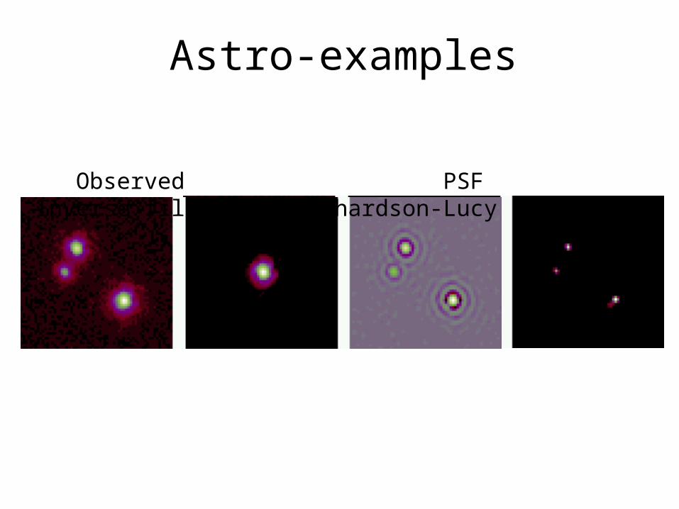
Astro-examples
Observed PSF Inverse filter Richardson-Lucy


