
Data StructuresLecture 11
Fang YuDepartment of Management Information SystemsNational Chengchi University
Fall 2010
A Review of Dynamic ProgrammingMain concepts:
The global optimum value can be defined in terms of optimal subproblems
The subproblems are not independent, but instead they overlap (hence, should be constructed bottom-up).
LCS problem: Given two strings X and Y, the longest common
subsequence (LCS) problem is to find a longest subsequence common to both X and Y

LCS Define L[i,j] to be the longest common
subsequence of X[0..i] and Y[0..j].
Allow for -1 as an index, so L[-1,k] = “” and L[k,-1]=“”, to indicate that the null part of X or Y has no match with the other.
Then we can define L[i,j] in the general case as follows:1. If xi=yj, then L[i,j] = L[i-1,j-1] + xi (we can
add this match)2. If xi≠yj, then L[i,j] = max{L[i-1,j], L[i,j-1]}
(we have no match here)

Search TreesBinary Search Trees, AVL trees, and Splay Trees

5
Binary Search TreesA binary search tree is a
binary tree storing keys (or key-value entries) at its internal nodes and satisfying the following property: Let u, v, and w be three
nodes such that u is in the left subtree of v and w is in the right subtree of v. We have key(u) key(v) key(w)
External nodes do not store items
An inorder traversal of a binary search trees visits the keys in increasing order
6
92
41 8

6
Search To search for a key k, we
trace a downward path starting at the root
The next node visited depends on the comparison of k with the key of the current node
If we reach a leaf, the key is not found
Example: get(4): Call TreeSearch(4,root)
The algorithms for floorEntry and ceilingEntry are similar
Algorithm TreeSearch(k, v)if T.isExternal (v)
return vif k < key(v)
return TreeSearch(k, T.left(v))else if k = key(v)
return velse { k > key(v) }
return TreeSearch(k, T.right(v)) 6
92
41 8
<
>=

7
InsertionTo perform operation
put(k, o), we search for key k (using TreeSearch)
Assume k is not already in the tree, and let w be the leaf reached by the search
We insert k at node w and expand w into an internal node
Example: insert 5
6
92
41 8
6
92
41 8
5
<
>
>
w
w

8
DeletionTo perform operation
remove(k), we search for key k
Assume key k is in the tree, and let let v be the node storing k
If node v has a leaf child w, we remove v and w from the tree with operation removeExternal(w), which removes w and its parent
Example: remove 4
6
92
41 8
5
vw
6
92
51 8
<
>
9
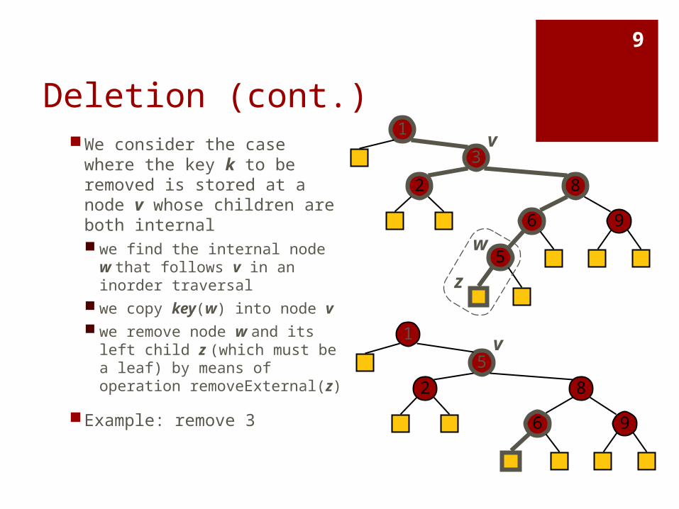
Deletion (cont.) We consider the case where
the key k to be removed is stored at a node v whose children are both internal we find the internal node w
that follows v in an inorder traversal
we copy key(w) into node v we remove node w and its
left child z (which must be a leaf) by means of operation removeExternal(z)
Example: remove 3
3
1
8
6 9
5
v
w
z
2
5
1
8
6 9
v
2

10
PerformanceConsider n ordered set
items implemented by means of a binary search tree of height h the space used is O(n) methods get, put and
remove take O(h) time
The height h is O(n) in the worst case and O(log n) in the best case
We want a balanced binary tree!

11
AVL Tree Definition
AVL trees are balanced
An AVL Tree is a binary search tree such that for every internal node v of T, the heights of the children of v can differ by at most 1
88
44
17 78
32 50
48 62
2
4
1
1
2
3
1
1
An example of an AVL tree where the heights are shown next to the nodes:

AVL Trees
12
Height of an AVL TreeFact: The height of an AVL tree storing n keys is O(log n).
Proof: Let us bound n(h): the minimum number of internal nodes of an AVL tree of height h.
We easily see that n(1) = 1 and n(2) = 2
For n > 2, an AVL tree of height h contains the root node, one AVL subtree of height n-1 and another of height n-2.
That is, n(h) = 1 + n(h-1) + n(h-2)
Knowing n(h-1) > n(h-2), we get n(h) > 2n(h-2). Son(h) > 2n(h-2), n(h) > 4n(h-4), n(h) > 8n(n-6), … (by induction),n(h) > 2in(h-2i)
Solving the base case we get: n(h) > 2 h/2-1
Taking logarithms: h < 2log n(h) +2
Thus the height of an AVL tree is O(log n)
3
4 n(1)
n(2)

13
Insertion Insertion is as in a binary search tree
Always done by expanding an external node.
Example: 44
17 78
32 50 88
48 62
54w
b=x
a=y
c=z
44
17 78
32 50 88
48 62
before insertion after insertion

After InsertionAll nodes along the path increase their height by 1
It may violate the AVL property44
17 78
32 50 88
48 62
54
44
17 78
32 50 88
48 62 1
2
4
3
1
2
3
4
5

Search and repairLet z be the first violation node from the
bottom along the path
Let y be z’child with the higher height (y is 2 greater than its sibling)
Let x be y’s child with the higher height
We rebalance z by calling trinode restructuring method

AVL Trees
16Trinode Restructuring
let (a,b,c) be an inorder listing of x, y, z
perform the rotations needed to make b the topmost node of the three
b=y
a=z
c=x
T0
T1
T2 T3
b=y
a=z c=x
T0 T1 T2 T3
c=y
b=x
a=z
T0
T1 T2
T3b=x
c=ya=z
T0 T1 T2 T3
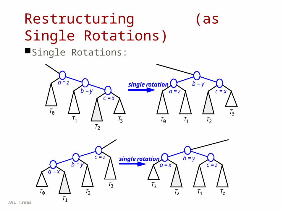
case 1: single rotation(a left rotation about a)
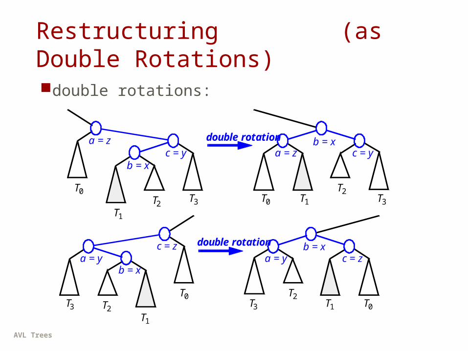
case 2: double rotation(a right rotation about c, then a left rotation about a)
(other two cases are symmetrical)
AVL Trees
17
Restructuring (as Single Rotations)Single Rotations:
T0T1
T2
T3
c = xb = y
a = z
T0 T1 T2
T3
c = xb = y
a = zsingle rotation
T3T2
T1
T0
a = xb = y
c = z
T0T1T2
T3
a = xb = y
c = zsingle rotation
AVL Trees
18
Restructuring (as Double Rotations)double rotations:
double rotationa = z
b = xc = y
T0T2
T1
T3 T0
T2T3T1
a = zb = x
c = y
double rotationc = z
b = xa = y
T0T2
T1
T3 T0
T2T3 T1
c = zb = x
a = y

AVL Trees
19Insertion Example, continued
88
44
17 78
32 50
48 62
2
5
1
1
3
4
2
1
54
1
T0T2
T3
x
y
z
2
3
4
5
67
1
88
44
17
7832 50
48
622
4
1
1
2 2
3
154
1
T0 T1
T2
T3
x
y z
unbalanced...
...balanced
1
2
3
4
5
6
7
T1
AVL Trees
20
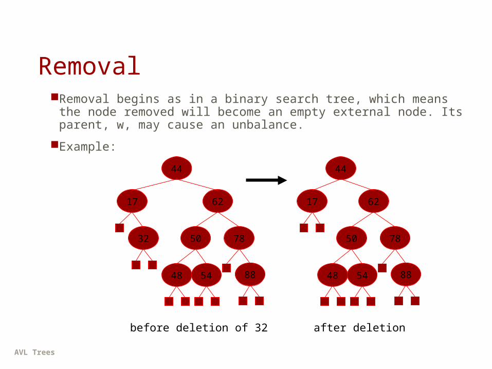
RemovalRemoval begins as in a binary search tree, which means the
node removed will become an empty external node. Its parent, w, may cause an unbalance.
Example:
44
17
7832 50
8848
62
54
44
17
7850
8848
62
54
before deletion of 32 after deletion

AVL Trees
21
Rebalancing after a Removal Let z be the first unbalanced node encountered while
travelling up the tree from w. Also, let y be the child of z with the larger height, and let x be the child of y with the larger height
As this restructuring may upset the balance of another node higher in the tree, we must continue checking for balance until the root of T is reached
44
17
7850
8848
62
54
w
c=x
b=y
a=z
44
17
78
50 88
48
62
54

22
AVL Tree Performancea single restructure takes O(1) time
using a linked-structure binary tree
get takes O(log n) timeheight of tree is O(log n), no restructures needed
put takes O(log n) time initial find is O(log n)Restructuring up the tree, maintaining heights is O(log n)
remove takes O(log n) time initial find is O(log n)Restructuring up the tree, maintaining heights is O(log n)

23
Splay Treea splay tree is a binary search tree where a
node is splayed after it is accessed (for a search or update)
deepest internal node accessed is splayed
splay: move the node to the root
splaying costs O(h), where h is height of the tree – which is still O(n) worst-case O(h) rotations, each of which is O(1)
24
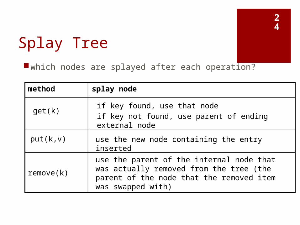
Splay Treewhich nodes are splayed after each operation?
use the parent of the internal node that was actually removed from the tree (the parent of the node that the removed item was swapped with)
remove(k)
use the new node containing the entry insertedput(k,v)
if key found, use that nodeif key not found, use parent of ending external node
get(k)
splay nodemethod

Splay Trees
25Searching in a Splay Tree:
Starts the Same as in a BST
Search proceeds down the tree to found item or an external node.
Example: Search for time with key 11.
(20,Z)
(37,P)(21,O)(14,J)
(7,T)
(35,R)(10,A)
(1,C)
(1,Q)
(5,G)(2,R)
(5,H)
(6,Y)(5,I)
(8,N)
(7,P)
(36,L)
(10,U)
(40,X)
Splay Trees
26
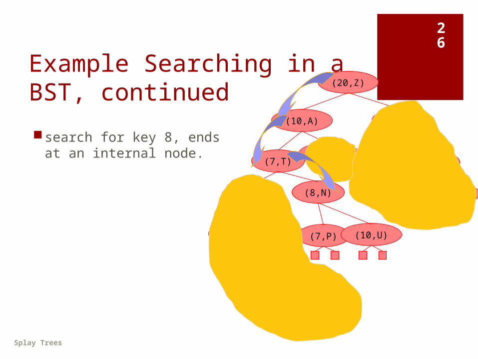
Example Searching in a BST, continued
search for key 8, ends at an internal node.
(20,Z)
(37,P)(21,O)(14,J)
(7,T)
(35,R)(10,A)
(1,C)
(1,Q)
(5,G)(2,R)
(5,H)
(6,Y)(5,I)
(8,N)
(7,P)
(36,L)
(10,U)
(40,X)

Splay Trees
27Splay Trees do Rotations after
Every Operation (Even Search)new operation: splay
splaying moves a node to the root using rotations right rotation
makes the left child x of a node y into y’s parent; y becomes the right child of x
y
x
T1 T2
T3
y
x
T1
T2T3
left rotation makes the right child y of a node x
into x’s parent; x becomes the left child of y
y
x
T1 T2
T3
y
x
T1
T2T3
(structure of tree above y is not modified)
(structure of tree above x is not modified)
a right rotation about y a left rotation about x

Splay Trees
28
Splaying:
is x the root?
stop
is x a child of the root?
right-rotate about the root
left-rotate about the root
is x the left child of the root?
is x a left-left grandchild?
is x a left-right grandchild?
is x a right-right grandchild?
is x a right-left grandchild?
right-rotate about g, right-rotate about p
left-rotate about g, left-rotate about p
left-rotate about p, right-rotate about g
right-rotate about p, left-rotate about g
start with node x
“x is a left-left grandchild” means x is a left child of its parent, which is itself a left child of its parent
p is x’s parent; g is p’s parent
no
yes
yes
yes
yes
yes
yes
no
no
yes zig-zig
zig-zag
zig-zag
zig-zig
zigzig

Splay Trees
29
Visualizing the Splaying Cases
zig-zag
y
x
T2 T3
T4
z
T1
y
x
T2 T3 T4
z
T1
y
x
T1 T2
T3
z
T4
zig-zig
y
z
T4T3
T2
x
T1
zig
x
w
T1 T2
T3
y
T4
y
x
T2 T3 T4
w
T1

Splay Trees
30
Splaying Example let x = (8,N)
x is the right child of its parent, which is the left child of the grandparent
left-rotate around p, then right-rotate around g
(20,Z)
(37,P)(21,O)(14,J)
(7,T)
(35,R)(10,A)
(1,C)
(1,Q)
(5,G)(2,R)
(5,H)
(6,Y)(5,I)
(8,N)
(7,P)
(36,L)
(10,U)
(40,X)
x
g
p
(10,A)
(20,Z)
(37,P)(21,O)
(35,R)
(36,L) (40,X)(7,T)
(1,C)
(1,Q)
(5,G)(2,R)
(5,H)
(6,Y)(5,I)
(14,J)(8,N)
(7,P)
(10,U)
x
g
p (10,A)
(20,Z)
(37,P)(21,O)
(35,R)
(36,L) (40,X)
(7,T)
(1,C)
(1,Q)
(5,G)(2,R)
(5,H)
(6,Y)(5,I)
(14,J)
(8,N)
(7,P)
(10,U)
x
g
p
1.(before rotating)
2.(after first rotation) 3.
(after second rotation)
x is not yet the root, so we splay again

Splay Trees
31Splaying Example, Continued
now x is the left child of the rootright-rotate around root
(10,A)
(20,Z)
(37,P)(21,O)
(35,R)
(36,L) (40,X)
(7,T)
(1,C)
(1,Q)
(5,G)(2,R)
(5,H)
(6,Y)(5,I)
(14,J)
(8,N)
(7,P)
(10,U)
x
(10,A)
(20,Z)
(37,P)(21,O)
(35,R)
(36,L) (40,X)
(7,T)
(1,C)
(1,Q)
(5,G)(2,R)
(5,H)
(6,Y)(5,I)
(14,J)
(8,N)
(7,P)
(10,U)
x
1.(before applying rotation)
2.(after rotation)
x is the root, so stop

Splay Trees
32Example Result
of Splaying tree might not be more balanced
e.g. splay (40,X) before, the depth of the shallowest leaf
is 3 and the deepest is 7 after, the depth of shallowest leaf is 1
and deepest is 8
(20,Z)
(37,P)(21,O)(14,J)
(7,T)
(35,R)(10,A)
(1,C)
(1,Q)
(5,G)(2,R)
(5,H)
(6,Y)(5,I)
(8,N)
(7,P)
(36,L)
(10,U)
(40,X)
(20,Z)
(37,P)
(21,O)
(14,J)(7,T)
(35,R)
(10,A)
(1,C)
(1,Q)
(5,G)(2,R)
(5,H)
(6,Y)(5,I)
(8,N)
(7,P) (36,L)(10,U)
(40,X)
(20,Z)
(37,P)
(21,O)
(14,J)(7,T)
(35,R)
(10,A)
(1,C)
(1,Q)
(5,G)(2,R)
(5,H)
(6,Y)(5,I)
(8,N)
(7,P)
(36,L)
(10,U)
(40,X)
before
after first splay after second splay

Splay Trees
33Performance of Splay
Trees
Amortized cost of any splay operation is O(log n)
This implies that splay trees can actually adapt to perform searches on frequently-requested items much faster than O(log n) in some cases

Project HintsHow to call google?
How to find the reference links?
How to encode Chinese?

HW11 (Due on Dec 1)Use Google and get the links!
Get a keyword from user
Return the urls listed in the search result
After this HW, you can step to the third stage of the project
You can apply the same technique to other search engines


