Data Modelling with Gaussian Process in Sensor Networks forUrban Environmental Monitoring
Xiuming Liu∗, Teng Xi†, Edith Ngai∗∗Department of Information Technology
Uppsala University, Uppsala, SwdenEmail: {xiuming.liu, edith.ngai}@it.uu.se
†State Key Laboratory of Networking and Switching TechnologyBeijing University of Posts and Telecommunications, Beijing, China
Email: [email protected]
Abstract—In this paper, the multidimensional output Gaus-sian process (GP) is applied to model urban environmental datacollected by sensor networks. Measurements from sensors atdifferent locations are correlated. Moreover, we observe thatthe pollution level in urban area is highly coupled with humanactivities and shows periodic patterns accordingly. Based onthese observations, we discuss the design of mean and kernelfunctions with two approaches: (1) composed kernel and max-imum likelihood estimation of hyper-parameters; (2) Wiener-Khinchin theorem based approximation of sample covariances.To validate the models, the accuracy of interpolations given bydifferent approaches are compared. The experimental resultsshow that, for the application of interpolation, the dependentGP with the approximated sample covariances as kernels canprovide better performance than the independent GP modelwith composed kernels.
Keywords-data modelling, Gaussian process, kernel design
I. INTRODUCTION
The global urbanization in recent decades has brought
more than half of the global population into cities, and
therefore produced many mega-cities worldwide. Urban en-
vironment pollution (especially air pollution) is one of the
major challenges for sustainable growth of our society. The
main air pollutants include carbon monoxide (CO), nitrogen
dioxide (NO2), and particulate matters (PM). According to
reports from World Health Organization (WHO) [1], long-
term exposure in highly polluted air environment leads to
several health risks, and consequently produces significant
economic costs for both individual citizen and the entire
society. Therefore, air quality information is important for
people who live in urban areas.
Many research projects have been conducted on develop-
ing urban environment monitoring systems [2, 3]. From the
quality of service (QoS) perspective, challenges of designing
sensor networks for urban environment monitoring exist
in two major aspects: data accuracy and service coverage.
The data accuracy is mostly determined by the quality
of sensing devices. For instance, the performance of low-
cost electrochemical sensors can be unstable (e.g., drift
of sensitivity) when the operating condition varies. The
challenge of service coverage appears when the energy and
density of sensor network are constrained, and therefore
available observations are often sparse in both time and
space. Interpolation [4] is a common approach to improve
the sensor network’s coverage. Most of data processing
methods require probabilistic models of the interested dy-
namics, which motivates our study in the this paper.
Gaussian process (GP) is a frequently used non-parametric
model in analysis of time series data. A GP is uniquely
defined by its mean and kernel functions. By carefully
designing the mean and kernel functions, we are able to
encode properties of the interested dynamics into the model.
Moreover, the multidimensional output GP (or dependent
GPs [5]) is capable of modelling the correlations between
measurements from different locations. The generality and
flexibility of GP makes it a powerful tool in time series
analysis [6]. In this work, we apply GP to model air
pollution data collected by sensor networks in urban area.
First, the multidimensional output GP model is defined for
sensor network data. Second, we present a kernel function
design approach based on the Wiener-Khinchin theorem.
Comparing to the likelihood based method, the Wiener-
Khinchin theorem based method can be totally automatic
and more computationally efficient.
The rest of this paper is organized as the following.
In section II, we review the related work for sensor data
modelling. A general GP model for sensor network data is
presented in section III. Next, in section IV, we discuss the
hidden periodic pattern in interested dynamics and different
approaches of designing mean and kernel functions. Exper-
imental results are shown in section V. Finally we conclude
this paper in section VI.
II. RELATED WORK
The data collected by different nodes in a sensor network
are often correlated in both time and space domains. These
correlations can be used as the side information when
processing sensor network data. Such idea has been explored
in the following previous works.
2016 IEEE 24th International Symposium on Modeling, Analysis and Simulation of Computer and Telecommunication Systems
2375-0227/16 $31.00 © 2016 IEEE
DOI 10.1109/MASCOTS.2016.45
457
Deshpande et al. [7] proposed a Bayesian probabilistic
model for data acquisition in sensor network, aiming to ex-
tend the lifetime of sensors by reducing the communication
and data acquisition costs. Since then the model-driven data
acquisition has become a popular approach in studies of
sensor network. Raza et al. [8] examines this methodology
and shows that the model driven approach does save the
energy, conditioning on coordinated operations of sensor
network. Thus, the critical task is to find a good probabilistic
data model which characterizes the interested dynamics.Gaussian process (GP) has been used widely in different
applications [9]. There are two key aspects of modelling
sensor network data with GP. Firstly, the GP model is
required to encode both temporal and spatial correlations of
sensor network data. One way of achieving this is to view
the measurements from different nodes as dependent (or
coupled) GPs [5]. In such cases, not only the auto-covariance
but also the cross-covariance functions are calculated in the
multidimensional output GP model. Secondly, appropriate
mean and kernel functions must be designed for measure-
ments from each sensor node (or pair of sensors in case
of cross-covariance), because measurements from different
sensors might have various patterns. Wilson summaries
commonly used basic kernels as well as the method of
constructing new kernels in his doctoral dissertation [10].
The evidence for designing kernel in the GP is usually
the sample covariance and estimated power spectrum. In
[11], the spectral mixture (SM) kernels is designed based on
Gaussian mixture approximation of power spectrum density.This paper distinguishes itself from the previous works in
the following aspects. First, we introduce a general frame-
work for sensor network data modelling based on multidi-
mensional output GP. The temporal and spatial correlations
of data are encoded in the multidimensional GP model
simultaneously. Second, we focus on cases where the data
collected by sensor network shows strong periodic patterns.
We compare the traditional likelihood based kernel function
design approach with the Wiener-Khinchin theorem based
approach, and show that the latter case is more efficient to
capture the hidden patterns and adapt to the training data.
III. SYSTEM MODEL
A. The Multidimensional Output GP
Let Xt =[x1t . . . xN
t
]Tbe the N -dimensional output
of a GP at the input of time stamp t:
Xt ∼ GP (m(t),k(t, t′)), (1)
where m(t) =[mx1(t) . . . mxN (t)
]Tis the vector of
mean functions, and the matrix k(t, t′) is given by⎡⎢⎢⎢⎣kx1,x1(t, t′) kx1,x2(t, t′) . . . kx1,xN (t, t′)kx2,x1(t, t′) kx2,x2(t, t′) . . . kx2,xN (t, t′)
......
. . ....
kxN ,x1(t, t′) kxN ,x2(t, t′) . . . kxN ,xN (t, t′)
⎤⎥⎥⎥⎦ . (2)
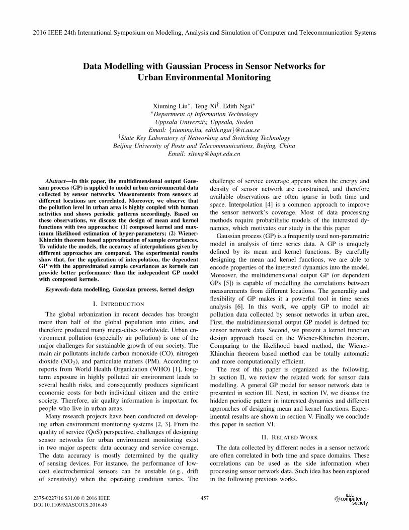
(a) Locations of sensors. (b) Correlation matrix.
Figure 1: An example of sensor network for urban air quality
monitoring and the scaled correlation matrix at Δt = 0.
The diagonal elements kxi,xi(t, t′) (i ∈ {1, . . . , N}) are
the auto-covariance functions; the non-diagonal elements
kxi,xj (t, t′) (i, j ∈ {1, . . . , N} and i �= j) are the cross-
covariances.
The model in Eq. (1) is also referred as N dependent (or
coupled) GPs [5]. In real-life scenarios, an output xit might
be coupled with a subset of the remaining outputs, resulting
in several elements in k(t, t′) close to matrices of zeros. In
the extreme case, an arbitrary dimension of outputs xit is
only dependent on itself. The matrix k(t, t′) will therefore
become diagonal and the coupled GP models becomes Nindependent one-dimensional output GPs.
B. Urban Sensor Network
Considering the planning of urban infrastructures (e.g.,
road systems) and different functions of districts of cities,
such as residential and industrial, the correlations between
sensors’ outputs are more complicate than the a function of
spatial distance. For example, two air pollution sensors de-
ployed at interchanges of city highway system might provide
highly correlated measurements, although their geographical
distance can be relatively large; while measurements from
other nodes, such as the ones deployed in the recreation area,
can be less correlated with the roadside sensors. An example
of deployment of air quality monitoring stations is showed
in Fig. 1a.
Denoting the measurements from N sensors as Xt =[x1t . . . xN
t
]T, the sensor data can be modelled as a N
dimensional output GP in Eq. (1). The auto-covariances of
measurements from a node i is characterized by the kernel
kxit,x
it(t, t′). The cross-covariance of measurements from
node i and node j is presented by the kernel kxi,xj (t, t′).Fig. 1b illustrates the covariance matrix in Eq. (2) evaluated
at zero time difference and scaled to [0, 1]. The diagonal ele-
ments are auto-covariance functions evaluated with zero lag,
resulting in maximum values. The non-diagonal elements
present various level of correlation. For example, nodes 3
and 4 have highest correlation among all pairs of sensors.
458

The mean function m(t) and kernel matrix k(t, t′) are
obtained from the historical data of the sensor network
(will be discussed in Section IV). Based on today’s wireless
communication and cloud computing technologies, it is
feasible to collect data from the sensor network and update
the GP model in a real time manner.
C. Joint Data Reconstruction
The urban sensor network for environmental monitoring
usually has long sampling periods, especially in the case
of battery powered sensor network where energy efficiency
must be considered. Therefore, to reconstruct the sensory
data from measurements with low sampling rate is an
important task.
In the following example, assume that measurements xit
and xjt from node i and j are available with a vector of
inputs t, we are interested in inferring values of outputs xit′
at unobserved inputs t′ from node i. The joint probability
of observations and unknown values, p(xit,x
jt,x
it′), is a
Gaussian distribution
N (
⎡⎣mi(t)mj(t)mi(t
′)
⎤⎦ ,
⎡⎣Kii(t, t) Kij(t, t) Kii(t, t
′)Kji(t, t) Kjj(t, t) Kji(t, t
′)Kii(t
′, t) Kij(t′, t) Kii(t
′, t′)
⎤⎦), (3)
and the conditional probability of unknown value is therefore
given by
p(xit′ |xi
t,xjt) ∼ N (μt′|t,Σt′|t), (4)
where μt′|t in Eq. (5) is the mean of estimation and Σt′|tin Eq. (6) is the covariance matrix. And xi
t′ = μt′|t is the
estimated value of unknown output xit′ .
IV. PERIODIC PATTERNS AND KERNEL DESIGN
A. Discover the Periodic Patterns
Before starting the discussion of designing mean and
kernel functions for the GP, we looked into a sequence of
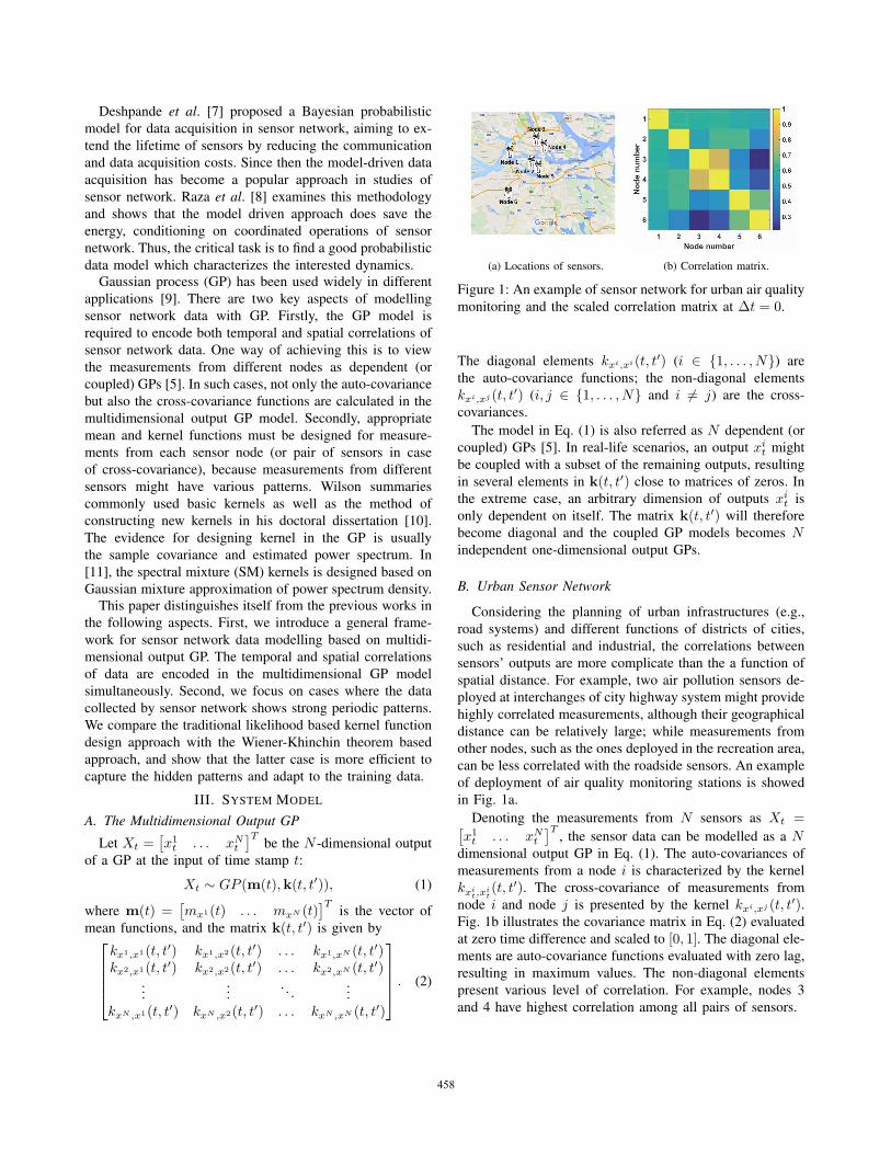
the measurements1, which are illustrated in Fig. 2. In this
example, node 1 (solid blue) is a station deployed on top
of a building’s roof, measuring the background air quality;
node 2 (dot red) is a station deployed on roadside in city
centre, measuring the local air quality.
The time series illustrated in Fig. 2 has two properties.
First, the value of this time series at any time stamp is
a random number with a distribution (mean and variance).
Hence the time series is stochastic process. Second, the time
series shows periodic patterns. At least 3 periodic patterns
can be discovered from the data showed in Fig. 2:
• Weekly pattern: the existence of weekly periodicity
cane be observed in the figure. The NO2 concentration
is lower during weekends and higher during weekdays.
• Daily pattern: consider 24 hours as a period, the NO2
concentration is lower at night and higher during day-
time.
1The data set is available at this website: http://slb.nu/elvf/
• Rush-hour pattern: hourly NO2 measurements within a
working day have two peaks, one is around 8:00 and
the other is around 17:00. This is due to the large traffic
volume and therefore high emission from vehicles.
In light of those three observations, next we discuss the
design of mean and kernel functions for the GP model.
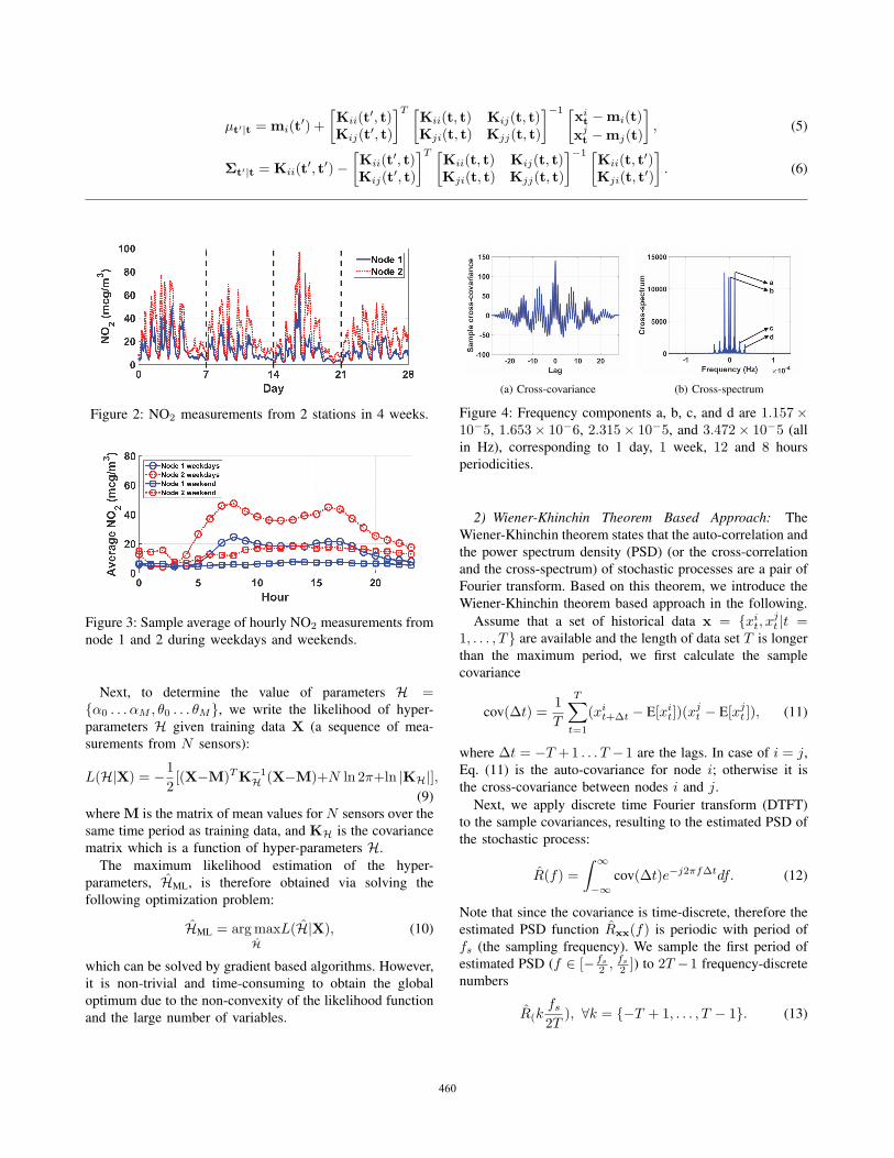
B. Design of Mean Function
Let’s consider a time series with the periodic pattern of pe-
riod Tp. Assume that a sequence of training data which con-
tains Np periods {xn∗Tp+t|n = 1, . . . , Np, t = 1, . . . , Tp}are available, the mean function of GP is designed to be
mx(kTp + t) =1
Np
Np−1∑n=0
xn∗Tp+t, ∀ k ∈ Z, (7)
where t ∈ {1, . . . , Tp} are the time indexes within one
period and k is the number of period. Equation (7) is
usually referred as the sample average estimator for the
mean function. The sample average is the minimum variance
unbiased (MVU) estimator for mean values of Gaussian
distribution [12]. In the example of NO2 measurements,
we separate the data set into weekdays and weekends, and
then apply Eq. (7) to calculate the averaged hourly NO2
measurements with Tp = 24 hours, which are illustrated in
Fig. 3.
Compared to the hourly average NO2 concentration dur-
ing weekends, the process during weekdays shows the
“double-peak” pattern, which is a reflection of rush-hours
during a working day.
C. Design of Kernel Function
The kernel function kxi,xj (t, t′) characterizes the correla-
tion of time series samples with distance Δt = t−t′. In case
of i = j, the kernel is also referred to the auto-covariance;
in case i �= j, the kernel represents the cross-covariance. We
discuss two approaches in the following: (1) likelihood based
approach, and (2) Wiener-Khinchin theorem based approach.
1) Likelihood Based Approach: The commonly used ap-
proach of kernel design is to first select a type of kernel,
and then determine the value of hyper-parameters in the
selected format via maximum likelihood estimation (MLE).
This approach is briefly reported in the following. We refer
readers to [9] for the details.
Assume that the stochastic process shows M periodic
patterns with periods {ω1, . . . , ωM}, a composed kernel [11]
can be designed as
M∑m=1
α2m exp[
− sin2(πωm(t− t′))2θ2m
] + α20 exp[
−(t− t′)2
2θ20],
(8)
which is a superposition of M basic periodic kernels of
different periodicities and a squared-exponential kernel.
459
μt′|t = mi(t′) +
[Kii(t
′, t)Kij(t
′, t)
]T [Kii(t, t) Kij(t, t)Kji(t, t) Kjj(t, t)
]−1 [xit −mi(t)
xjt −mj(t)
], (5)
Σt′|t = Kii(t′, t′)−
[Kii(t
′, t)Kij(t
′, t)
]T [Kii(t, t) Kij(t, t)Kji(t, t) Kjj(t, t)
]−1 [Kii(t, t
′)Kji(t, t
′)
]. (6)
Figure 2: NO2 measurements from 2 stations in 4 weeks.
Figure 3: Sample average of hourly NO2 measurements from
node 1 and 2 during weekdays and weekends.
Next, to determine the value of parameters H ={α0 . . . αM , θ0 . . . θM}, we write the likelihood of hyper-
parameters H given training data X (a sequence of mea-
surements from N sensors):
L(H|X) = −1
2[(X−M)TK−1
H (X−M)+N ln 2π+ln |KH|],(9)
where M is the matrix of mean values for N sensors over the
same time period as training data, and KH is the covariance
matrix which is a function of hyper-parameters H.
The maximum likelihood estimation of the hyper-
parameters, HML, is therefore obtained via solving the
following optimization problem:
HML = argmaxH
L(H|X), (10)
which can be solved by gradient based algorithms. However,
it is non-trivial and time-consuming to obtain the global
optimum due to the non-convexity of the likelihood function
and the large number of variables.
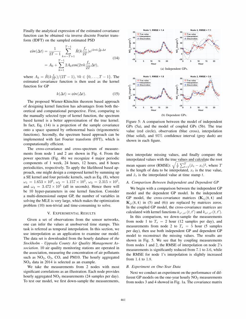
(a) Cross-covariance (b) Cross-spectrum
Figure 4: Frequency components a, b, c, and d are 1.157×10⁻⁵, 1.653× 10⁻⁶, 2.315× 10⁻⁵, and 3.472× 10⁻⁵ (all
in Hz), corresponding to 1 day, 1 week, 12 and 8 hours
periodicities.
2) Wiener-Khinchin Theorem Based Approach: The
Wiener-Khinchin theorem states that the auto-correlation and
the power spectrum density (PSD) (or the cross-correlation
and the cross-spectrum) of stochastic processes are a pair of
Fourier transform. Based on this theorem, we introduce the
Wiener-Khinchin theorem based approach in the following.
Assume that a set of historical data x = {xit, x
jt |t =
1, . . . , T} are available and the length of data set T is longer
than the maximum period, we first calculate the sample
covariance
cov(Δt) =1
T
T∑t=1
(xit+Δt − E[xi
t])(xjt − E[xj
t ]), (11)
where Δt = −T +1 . . . T −1 are the lags. In case of i = j,
Eq. (11) is the auto-covariance for node i; otherwise it is
the cross-covariance between nodes i and j.
Next, we apply discrete time Fourier transform (DTFT)
to the sample covariances, resulting to the estimated PSD of
the stochastic process:
R(f) =
∫ ∞
−∞cov(Δt)e−j2πfΔtdf. (12)
Note that since the covariance is time-discrete, therefore the
estimated PSD function Rxx(f) is periodic with period of
fs (the sampling frequency). We sample the first period of
estimated PSD (f ∈ [− fs2 ,
fs2 ]) to 2T −1 frequency-discrete
numbers
R(kfs2T
), ∀k = {−T + 1, . . . , T − 1}. (13)
460
Finally the analytical expression of the estimated covariance
function can be obtained via inverse discrete Fourier trans-
form (IDFT) on the sampled estimated PSD
ˆcov(Δt) =1
2T − 1
T−1∑k=−T+1
R(kfs2T
)ej2πkfs2T Δt
= A0 +T−1∑k=1
2Akcos(2πkfs2T
Δt),
(14)
where Ak = R(k fs2T )/(2T − 1), ∀k ∈ {0, . . . , T − 1}. The
estimated covariance function is then used as the kernel
function for GP
k(Δt) = ˆcov(Δt). (15)
The proposed Wiener-Khinchin theorem based approach
of designing kernel function has advantages from both the-
oretical and computational perspective. First, comparing to
the manually selected type of kernel function, the spectrum
based kernel is a better approximation of the true kernel.
In fact, Eq. (14) is a projection of the sample covariance
onto a space spanned by orthonormal basis (trigonometric
functions). Secondly, the spectrum based approach can be
implemented with fast Fourier transform (FFT), which is
computationally efficient.
The cross-covariance and cross-spectrum of measure-
ments from node 1 and 2 are shown in Fig. 4. From the
power spectrum (Fig. 4b) we recognize 4 major periodic
components of 1 week, 24 hours, 12 hours, and 8 hours
periodicities, respectively. To apply the likelihood based ap-
proach, one might design a composed kernel by summing up
a SE kernel and four periodic kernels, such as Eq. (8), where
ω1 = 1.653× 10⁶, ω2 = 1.157× 10⁵, ω3 = 2.315× 10⁵,
and ω4 = 3.472× 10⁵ (all in seconds). Hence there will
be 10 hyper-parameters in one kernel function. Consider
a multi-dimensional output GP, the number of variables in
solving the MLE is very large, which makes the optimization
problem (10) non-trivial and time-consuming to solve.
V. EXPERIMENTAL RESULTS
Given a set of observations from the sensor networks,
one can infer the values at unobserved time stamps. This
task is referred as temporal interpolation. In this section, we
use interpolation as an application to examine our model.
The data set is downloaded from the hourly database of theStockholm - Uppsala County Air Quality Management As-sociation. 10 air quality monitoring stations are operated in
the association, measuring the concentration of air pollutants
such as NO2, O3, CO, and PM10. The hourly aggregated
NO2 data in 2014 is selected as an example.
We take the measurements from 2 nodes with most
significant correlations as an illustration. Each node provides
hourly aggregated NO2 measurements (24 samples per day).
To test our model, we first down-sample the measurements,
(a) Independent GPs.
(b) Dependent GPs.
Figure 5: A comparison between the model of independent
GPs (5a), and the model of coupled GPs (5b). The true
value (red circle), observation (blue cross), interpolation
(blue solid), and 95% confidence interval (grey dash) are
shown in each figure.
then interpolate missing values, and finally compare the
interpolated values with the true values and calculate the root
mean square error (RMSE):
√1T
∑Tt=1(xt − xt)2, where T
is the length of data to be interpolated, xt is the true value,
and xt is the interpolated value at time stamp t.
A. Comparison Between Independent and Dependent GP
We begin with a comparison between the independent GP
model and the dependent GP model. In the independent
GP model, the cross-covariance matrices (Kij(t, t) and
Kji(t, t) in (5) and (6)) are replaced by matrices zeros.
In the coupled GP model, the cross-covariance matrices are
calculated with kernel functions kxi,xj (t, t′) and kxj ,xi(t, t′).In this comparison, we down-sample the measurements
from node 1 to Ts = 2 hour (12 samples per day), and
measurements from node 2 to Ts = 5 hour (5 samples
per day), then use both independent GP and dependent GP
model to reconstruct the missing values. The results are
shown in Fig. 5. We see that by coupling measurements
from nodes 1 and 2, the RMSE of interpolation on node 2’s
measurements is significantly reduced from 7.1 to 3.6, while
the RMSE for node 1’s interpolation is slightly increased
from 1.4 to 1.8.
B. Experiment on One-Year Data
Next we conduct an experiment on the performance of dif-
ferent GP models on the one-year hourly NO2 measurements
from nodes 3 and 4 showed in Fig. 1a. The covariance matrix
461
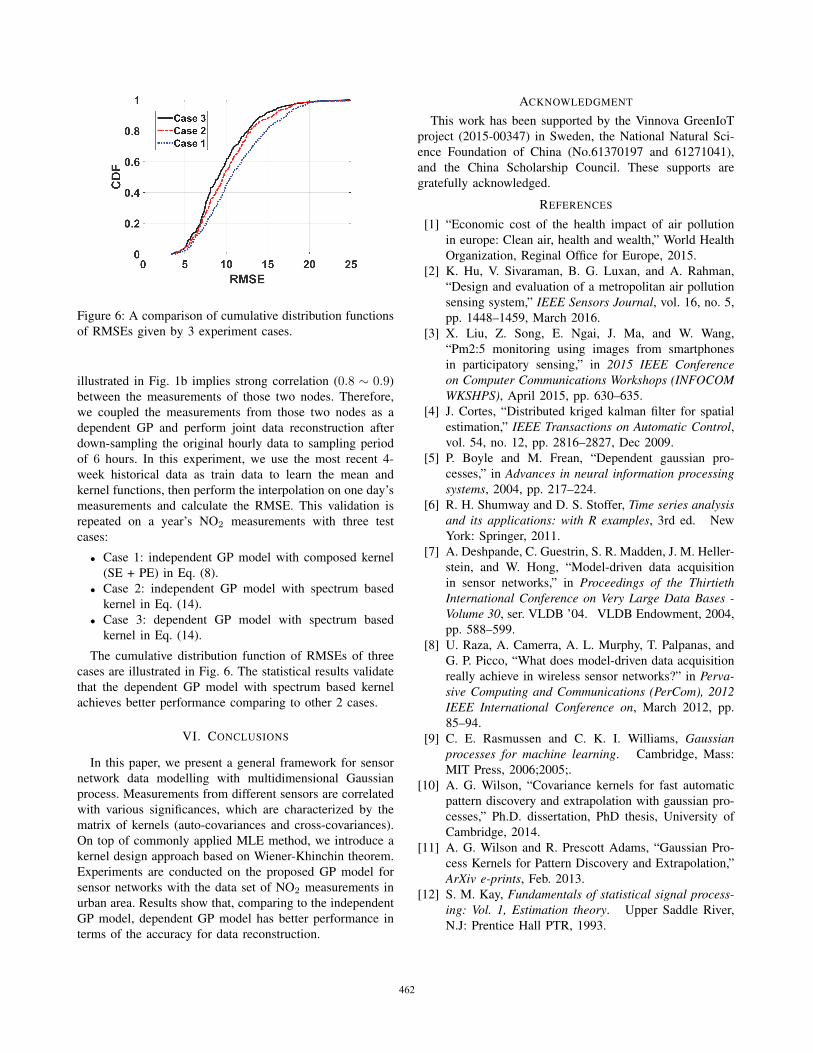
Figure 6: A comparison of cumulative distribution functions
of RMSEs given by 3 experiment cases.
illustrated in Fig. 1b implies strong correlation (0.8 ∼ 0.9)
between the measurements of those two nodes. Therefore,
we coupled the measurements from those two nodes as a
dependent GP and perform joint data reconstruction after
down-sampling the original hourly data to sampling period
of 6 hours. In this experiment, we use the most recent 4-
week historical data as train data to learn the mean and
kernel functions, then perform the interpolation on one day’s
measurements and calculate the RMSE. This validation is
repeated on a year’s NO2 measurements with three test
cases:
• Case 1: independent GP model with composed kernel
(SE + PE) in Eq. (8).
• Case 2: independent GP model with spectrum based
kernel in Eq. (14).
• Case 3: dependent GP model with spectrum based
kernel in Eq. (14).
The cumulative distribution function of RMSEs of three
cases are illustrated in Fig. 6. The statistical results validate
that the dependent GP model with spectrum based kernel
achieves better performance comparing to other 2 cases.
VI. CONCLUSIONS
In this paper, we present a general framework for sensor
network data modelling with multidimensional Gaussian
process. Measurements from different sensors are correlated
with various significances, which are characterized by the
matrix of kernels (auto-covariances and cross-covariances).
On top of commonly applied MLE method, we introduce a
kernel design approach based on Wiener-Khinchin theorem.
Experiments are conducted on the proposed GP model for
sensor networks with the data set of NO2 measurements in
urban area. Results show that, comparing to the independent
GP model, dependent GP model has better performance in
terms of the accuracy for data reconstruction.
ACKNOWLEDGMENT
This work has been supported by the Vinnova GreenIoT
project (2015-00347) in Sweden, the National Natural Sci-
ence Foundation of China (No.61370197 and 61271041),
and the China Scholarship Council. These supports are
gratefully acknowledged.
REFERENCES
[1] “Economic cost of the health impact of air pollution
in europe: Clean air, health and wealth,” World Health
Organization, Reginal Office for Europe, 2015.
[2] K. Hu, V. Sivaraman, B. G. Luxan, and A. Rahman,
“Design and evaluation of a metropolitan air pollution
sensing system,” IEEE Sensors Journal, vol. 16, no. 5,
pp. 1448–1459, March 2016.
[3] X. Liu, Z. Song, E. Ngai, J. Ma, and W. Wang,
“Pm2:5 monitoring using images from smartphones
in participatory sensing,” in 2015 IEEE Conferenceon Computer Communications Workshops (INFOCOMWKSHPS), April 2015, pp. 630–635.
[4] J. Cortes, “Distributed kriged kalman filter for spatial
estimation,” IEEE Transactions on Automatic Control,vol. 54, no. 12, pp. 2816–2827, Dec 2009.
[5] P. Boyle and M. Frean, “Dependent gaussian pro-
cesses,” in Advances in neural information processingsystems, 2004, pp. 217–224.
[6] R. H. Shumway and D. S. Stoffer, Time series analysisand its applications: with R examples, 3rd ed. New
York: Springer, 2011.
[7] A. Deshpande, C. Guestrin, S. R. Madden, J. M. Heller-
stein, and W. Hong, “Model-driven data acquisition
in sensor networks,” in Proceedings of the ThirtiethInternational Conference on Very Large Data Bases -Volume 30, ser. VLDB ’04. VLDB Endowment, 2004,
pp. 588–599.
[8] U. Raza, A. Camerra, A. L. Murphy, T. Palpanas, and
G. P. Picco, “What does model-driven data acquisition
really achieve in wireless sensor networks?” in Perva-sive Computing and Communications (PerCom), 2012IEEE International Conference on, March 2012, pp.
85–94.
[9] C. E. Rasmussen and C. K. I. Williams, Gaussianprocesses for machine learning. Cambridge, Mass:
MIT Press, 2006;2005;.
[10] A. G. Wilson, “Covariance kernels for fast automatic
pattern discovery and extrapolation with gaussian pro-
cesses,” Ph.D. dissertation, PhD thesis, University of
Cambridge, 2014.
[11] A. G. Wilson and R. Prescott Adams, “Gaussian Pro-
cess Kernels for Pattern Discovery and Extrapolation,”
ArXiv e-prints, Feb. 2013.
[12] S. M. Kay, Fundamentals of statistical signal process-ing: Vol. 1, Estimation theory. Upper Saddle River,
N.J: Prentice Hall PTR, 1993.
462


