Data Analytics for South West Area Health Pathology
Dr. David DaviesJason Chen
Prof. Jon PatrickRitika Sharma
Yu Xia

Agenda• Motivation• Research questions
– Appendix– Kidney– Vasculitis
• Move SWAPS from Mysql to Postgres• Postgres and Mysql Performance Comparision• Conclusion• CLINIDAL Comparison• Future Work
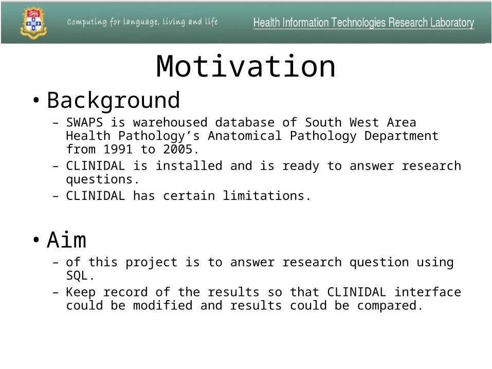
Motivation• Background
– SWAPS is warehoused database of South West Area Health Pathology’s Anatomical Pathology Department from 1991 to 2005.
– CLINIDAL is installed and is ready to answer research questions.
– CLINIDAL has certain limitations.
• Aim – of this project is to answer research question using SQL. – Keep record of the results so that CLINIDAL interface could be
modified and results could be compared.

Research Questions
• Appendix
• Kidney Glomerular Disease
• Vasculitis
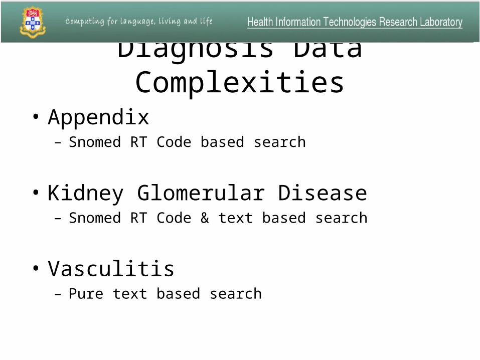
Diagnosis Data Complexities
• Appendix– Snomed RT Code based search
• Kidney Glomerular Disease– Snomed RT Code & text based search
• Vasculitis– Pure text based search
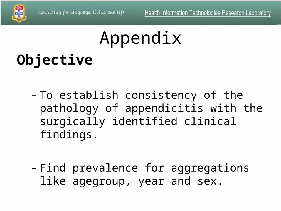
AppendixObjective
– To establish consistency of the pathology of appendicitis with the surgically identified clinical findings.
– Find prevalence for aggregations like agegroup, year and sex.
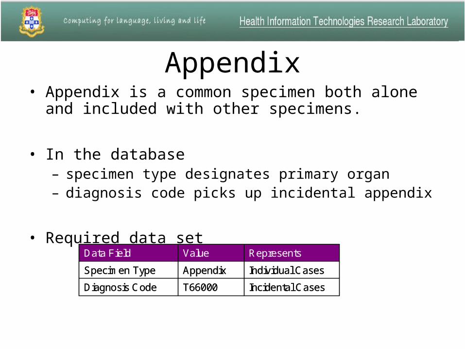
Appendix• Appendix is a common specimen both alone and
included with other specimens.
• In the database – specimen type designates primary organ– diagnosis code picks up incidental appendix
• Required data set
Incidental CasesT66000Diagnosis Code
Individual CasesAppendixSpecimen Type
RepresentsValueData Field
Incidental CasesT66000Diagnosis Code
Individual CasesAppendixSpecimen Type
RepresentsValueData Field
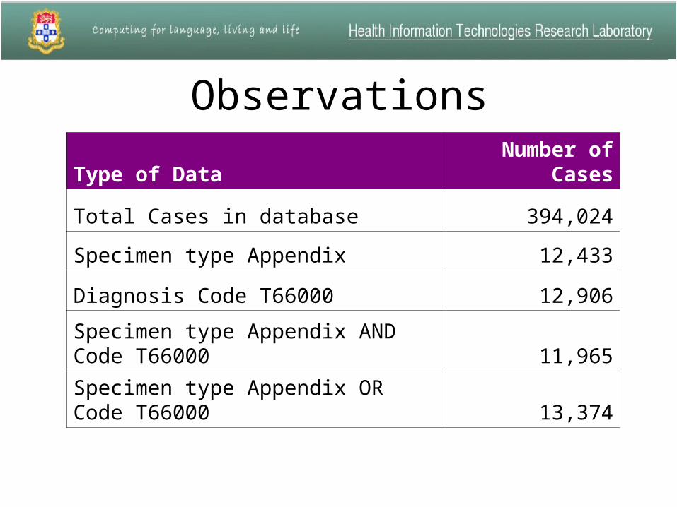
Observations
Type of DataNumber of
Cases
Total Cases in database 394,024
Specimen type Appendix 12,433
Diagnosis Code T66000 12,906
Specimen type Appendix AND Code T66000 11,965
Specimen type Appendix OR Code T66000 13,374
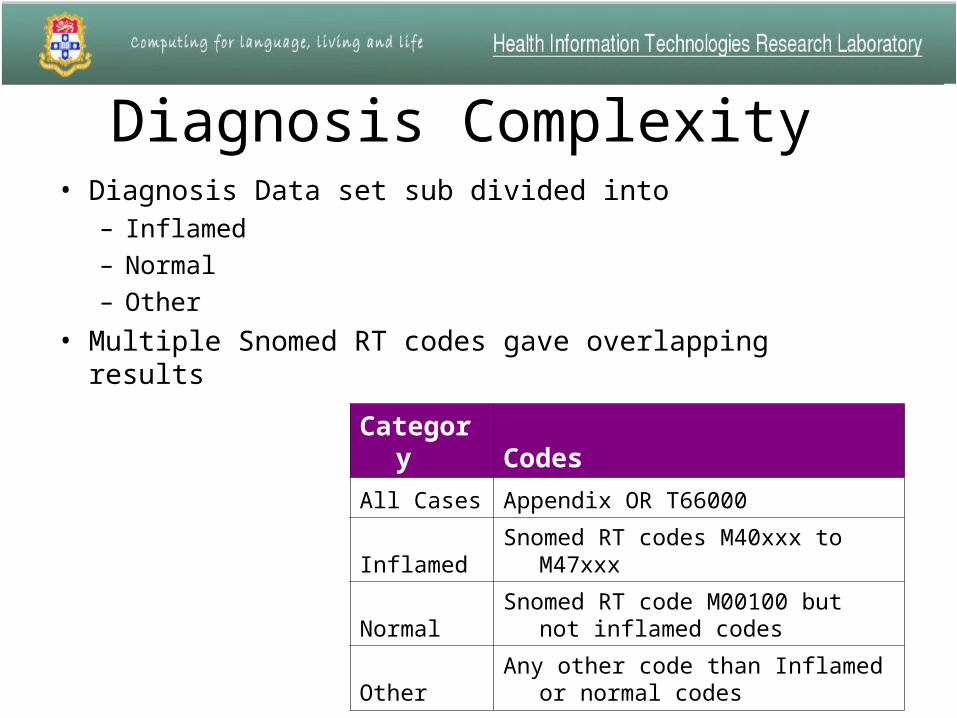
Diagnosis Complexity • Diagnosis Data set sub divided into
– Inflamed
– Normal
– Other
• Multiple Snomed RT codes gave overlapping results
Category Codes
All Cases Appendix OR T66000
Inflamed Snomed RT codes M40xxx to M47xxx
NormalSnomed RT code M00100 but not
inflamed codes
OtherAny other code than Inflamed or
normal codes

Appendix category distribution% of appendix sample
Inflamed72%
Normal 19%
Others9%
Inflamed
Normal
Others
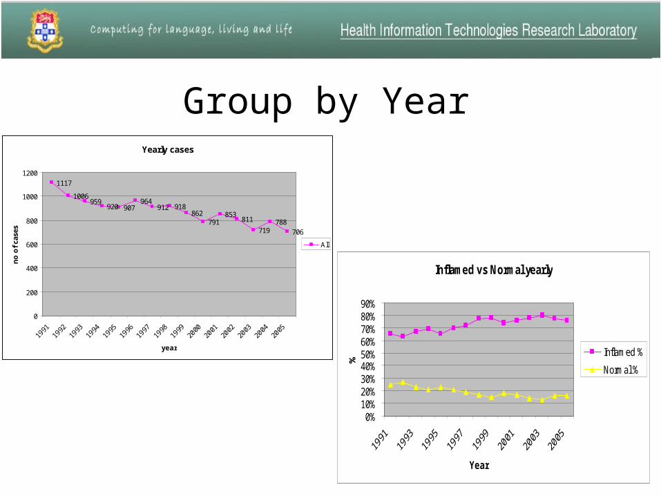
Inflamed vs Normal yearly
0%10%20%30%40%50%60%70%80%90%
Year
%Inflamed %
Normal %
Group by YearYearly cases
1117
1006959
920 907964
912 918862
791853
811
719788
706
0
200
400
600
800
1000
1200
year
no
of
case
s
All
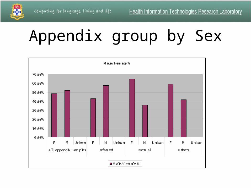
Appendix group by Sex
Male/ Female %
0.00%
10.00%
20.00%
30.00%
40.00%
50.00%
60.00%
70.00%
F M Unkwn F M Unkwn F M Unkwn F M Unkwn
All appendix Samples Inflamed Normal Others
Male/ Female %
Appendix Summary
• Wrong coding, Normal cases coded as Inflamed or vice versa
• Snomed RT codes were not grouped, inflamed in other organ and normal for appendix will put in Inflamed category.
• Many other category cases could fit into normal cases e.g. Faecolith, Pinworm etc.
Kidney Glomerular Disease• Objective
– To identify distribution of glomerular disease among its different sub types.
– Find association of glomerular disease with Transplant and Tubulointerstitial disease

Kidney Glomerular Disease• Glomerular disease is the main reason why kidney/renal biopsy is
done.
• There are three stages of renal biopsy:
1. Histology2. Immunoflorescence3. Electron microscopy
• Some diagnosis require all three to get a final diagnosis
– Histology is fast, Electron microscopy takes time.
– In many reports after histology diagnosis may remain as morphology only or list possibilities.
– In this study we are considering histology reports only.

Diagnosis Data set• Data set was extracted three ways:
– All cases with specimen type Renal Biop(sy) (86%)
– All cases where specimen type was not Renal Biop(sy) but in the text there was ‘Renal Biopsy’ or ‘Renal Bx’ (13%)
– Cases which don’t fall under above two conditions and have some common bigrams in the text report (1%).
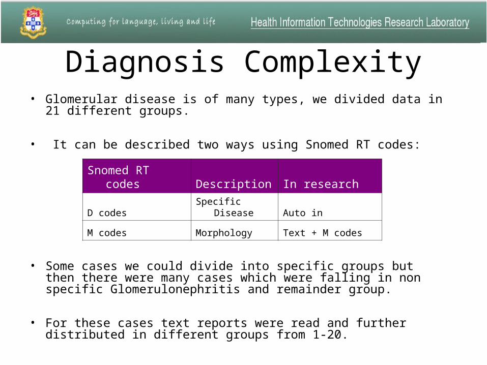
Diagnosis Complexity• Glomerular disease is of many types, we divided data in 21
different groups.
• It can be described two ways using Snomed RT codes:
• Some cases we could divide into specific groups but then there were many cases which were falling in non specific Glomerulonephritis and remainder group.
• For these cases text reports were read and further distributed in different groups from 1-20.
Snomed RT codes Description In research
D codes Specific Disease Auto in
M codes Morphology Text + M codes
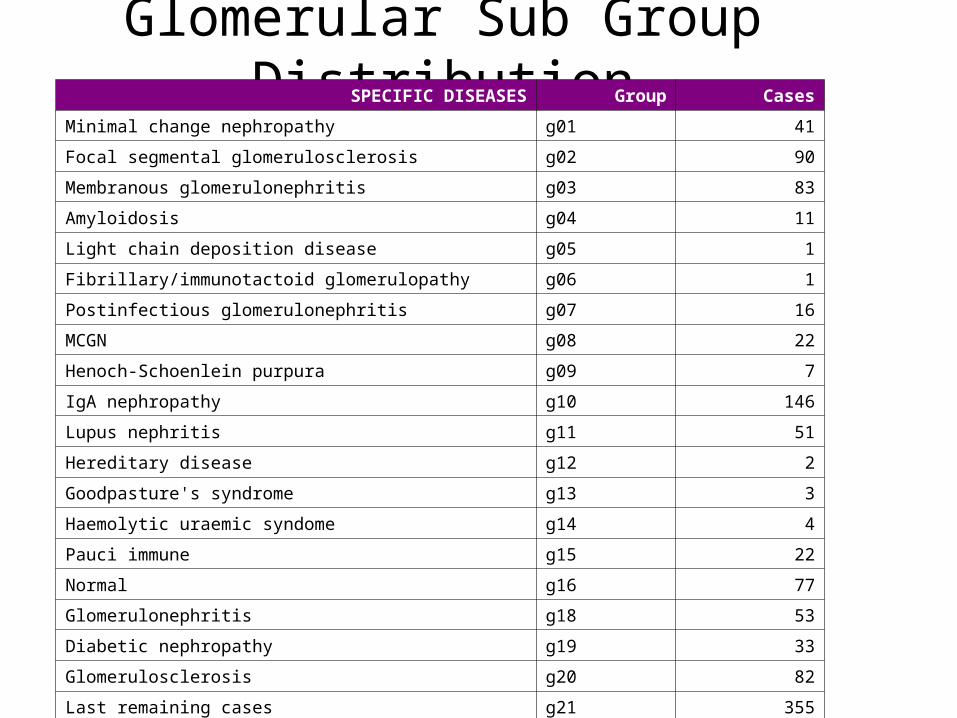
Glomerular Sub Group DistributionSPECIFIC DISEASES Group Cases
Minimal change nephropathy g01 41
Focal segmental glomerulosclerosis g02 90
Membranous glomerulonephritis g03 83
Amyloidosis g04 11
Light chain deposition disease g05 1
Fibrillary/immunotactoid glomerulopathy g06 1
Postinfectious glomerulonephritis g07 16
MCGN g08 22
Henoch-Schoenlein purpura g09 7
IgA nephropathy g10 146
Lupus nephritis g11 51
Hereditary disease g12 2
Goodpasture's syndrome g13 3
Haemolytic uraemic syndome g14 4
Pauci immune g15 22
Normal g16 77
Glomerulonephritis g18 53
Diabetic nephropathy g19 33
Glomerulosclerosis g20 82
Last remaining cases g21 355
Total 1100
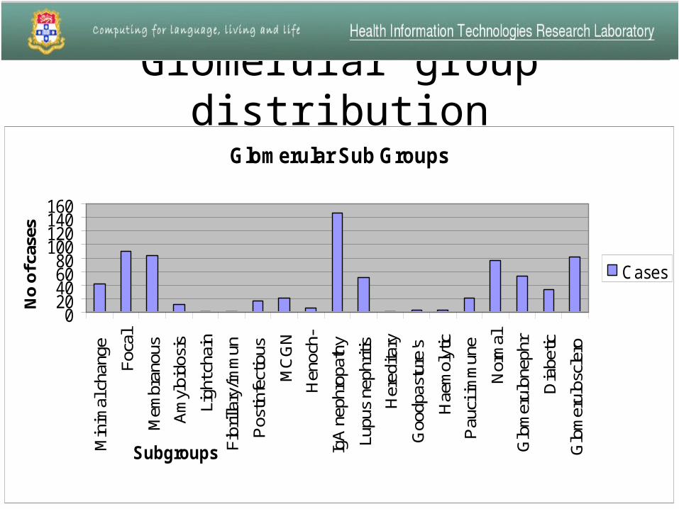
Glomerular group distribution
Glomerular Sub Groups
020406080
100120140160
Min
imal
cha
nge
Foca
l
Mem
bran
ous
Am
yloi
dosi
s
Ligh
t cha
in
Fibr
illar
y/im
mun
Pos
tinfe
ctio
us
MC
GN
Hen
och-
IgA
nep
hrop
athy
Lupu
s ne
phrit
is
Her
edita
ry
Goo
dpas
ture
's
Hae
mol
ytic
Pau
ci im
mun
e
Nor
mal
Glo
mer
ulon
ephr
Dia
betic
Glo
mer
ulos
cler
o
Subgroups
No
of c
ases
Cases
Kidney Summary• As this was text and code based search, we would have
picked only those cases which were consistently reported well along with correct codes.
• 14% samples were not entered under specimen type renal biopsy.
• We did not consider negation in text search.
• Many diagnosis require clinical history to interpret eg. No abnormality seen is “normal”, if protein in urine then its consistent with “minimal change disease”

Vasculitis• Objective
– Identify the prevalence of Vasculitis. What organs do they turn up in?
– Distribution of Vasculitis among its subtypes.

Vasculitis
• General term for a group of uncommon diseases that feature inflammation of the blood vessels.
• There are no specific diagnosis codes for this disease.
• The data set for this study will include all cases in database and its 100% text based search.
• NLP comes into action here as we need to be able to handle negation.
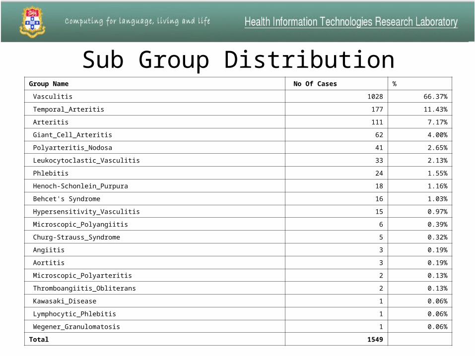
Sub Group DistributionGroup Name No Of Cases %
Vasculitis 1028 66.37%
Temporal_Arteritis 177 11.43%
Arteritis 111 7.17%
Giant_Cell_Arteritis 62 4.00%
Polyarteritis_Nodosa 41 2.65%
Leukocytoclastic_Vasculitis 33 2.13%
Phlebitis 24 1.55%
Henoch-Schonlein_Purpura 18 1.16%
Behcet's Syndrome 16 1.03%
Hypersensitivity_Vasculitis 15 0.97%
Microscopic_Polyangiitis 6 0.39%
Churg-Strauss_Syndrome 5 0.32%
Angiitis 3 0.19%
Aortitis 3 0.19%
Microscopic_Polyarteritis 2 0.13%
Thromboangiitis_Obliterans 2 0.13%
Kawasaki_Disease 1 0.06%
Lymphocytic_Phlebitis 1 0.06%
Wegener_Granulomatosis 1 0.06%
Total 1549
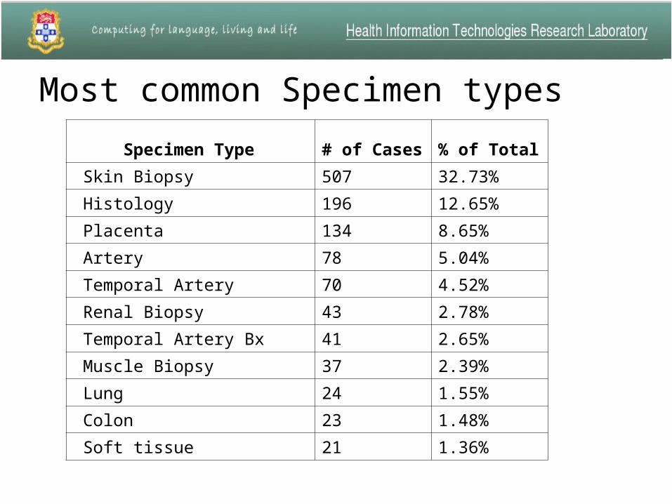
Most common Specimen types
Specimen Type # of Cases % of Total
Skin Biopsy 507 32.73%
Histology 196 12.65%
Placenta 134 8.65%
Artery 78 5.04%
Temporal Artery 70 4.52%
Renal Biopsy 43 2.78%
Temporal Artery Bx 41 2.65%
Muscle Biopsy 37 2.39%
Lung 24 1.55%
Colon 23 1.48%
Soft tissue 21 1.36%
Vasculitis Summary• As this was pure text based search, handling negation was a big challenge.
• While doing text search we found that in the report text, when ever sentence was rolling over to next line there was extra new line character, which was limiting our results when the phrase we were looking for were in two line.
• Some of the group names had common name in them so we have duplicate records, nearly 20%
• We started with 3466 unique cases and reduced them down to 1536 unique cases using few common negative terms, that was reduction of 55%.
• We believe this number will go further down once we compute this using CLINIDAL.

Move SWAPS from mysql to postgresql
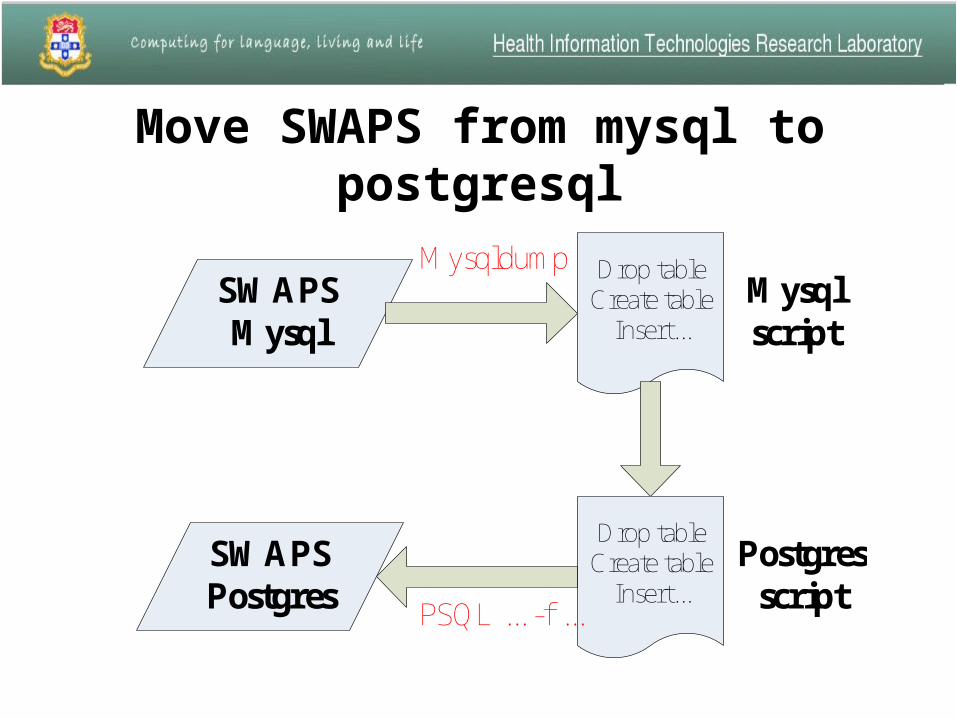
Move SWAPS from mysql to postgresql
SWAPSMysql
Drop tableCreate table
Insert...
Drop tableCreate table
Insert...
SWAPSPostgres
Mysql script
Postgresscript
Mysqldump
PSQL ... -f ...
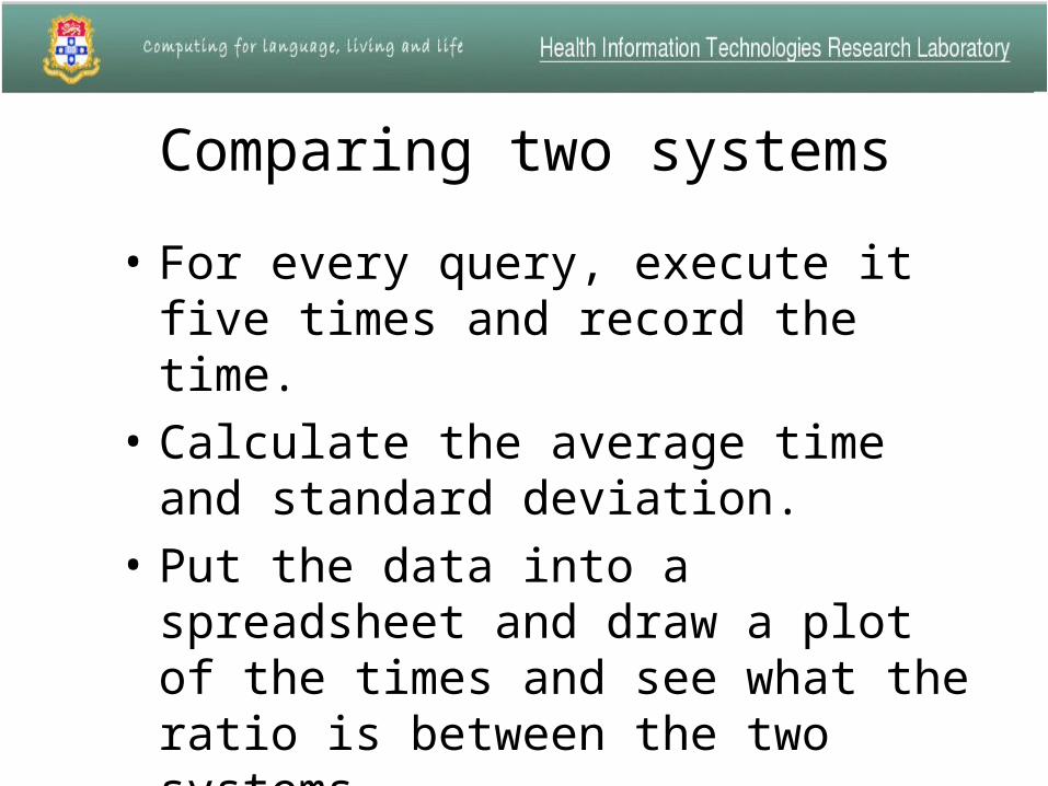
Comparing two systems
• For every query, execute it five times and record the time.
• Calculate the average time and standard deviation.
• Put the data into a spreadsheet and draw a plot of the times and see what the ratio is between the two systems.
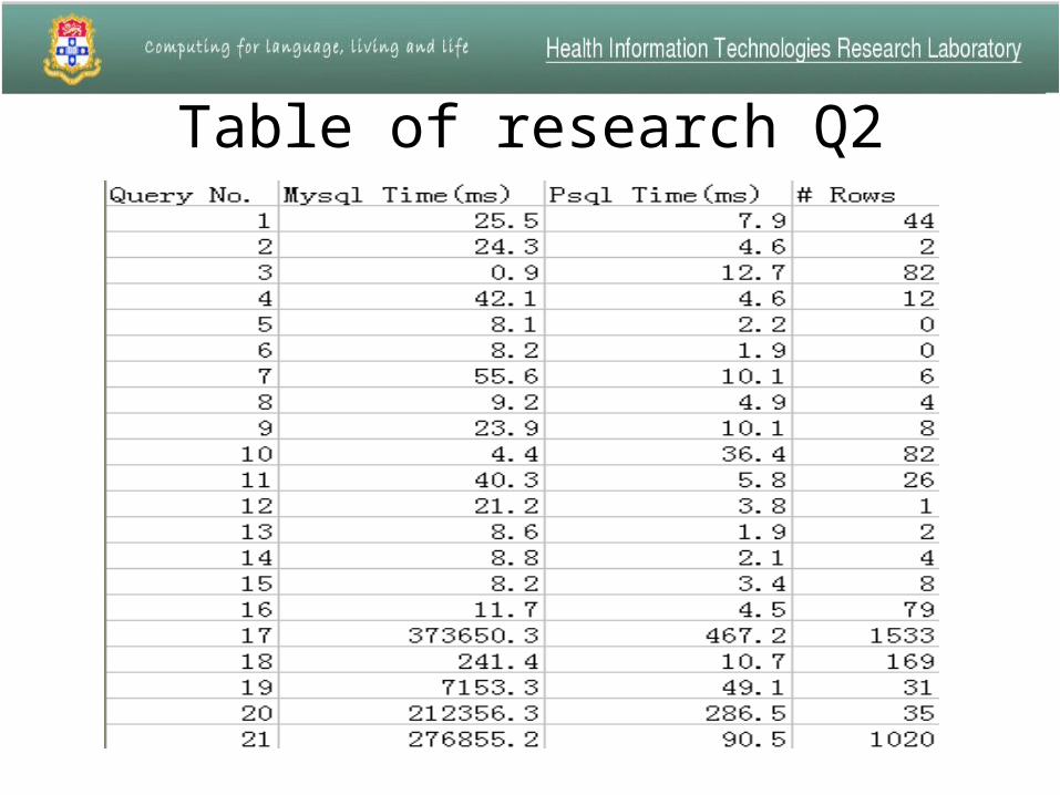
Table of research Q2
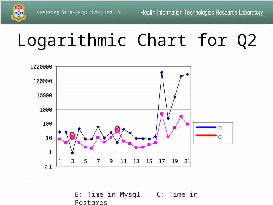
Logarithmic Chart for Q2
0.1
1
10
100
1000
10000
100000
1000000
1 3 5 7 9 11 13 15 17 19 21
B: Time in Mysql C: Time in Postgres
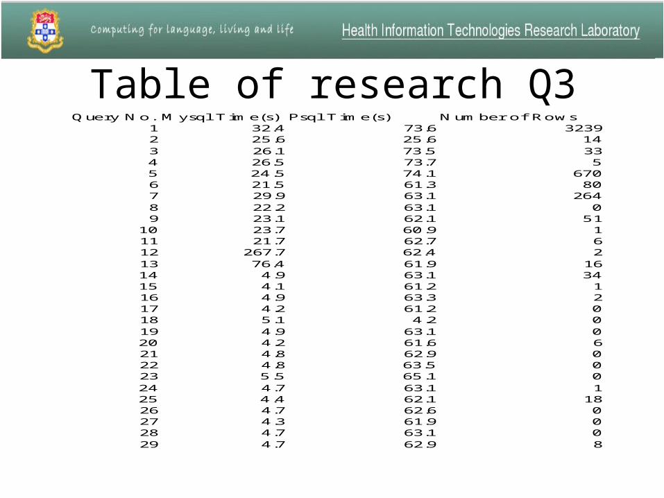
Table of research Q3Query No. Mysql T ime(s) Psql T ime(s) Number of Rows
1 32.4 73.6 32392 25.6 25.6 143 26.1 73.5 334 26.5 73.7 55 24.5 74.1 6706 21.5 61.3 807 29.9 63.1 2648 22.2 63.1 09 23.1 62.1 51
10 23.7 60.9 111 21.7 62.7 612 267.7 62.4 213 76.4 61.9 1614 4.9 63.1 3415 4.1 61.2 116 4.9 63.3 217 4.2 61.2 018 5.1 4.2 019 4.9 63.1 020 4.2 61.6 621 4.8 62.9 022 4.8 63.5 023 5.5 65.1 024 4.7 63.1 125 4.4 62.1 1826 4.7 62.6 027 4.3 61.9 028 4.7 63.1 029 4.7 62.9 8
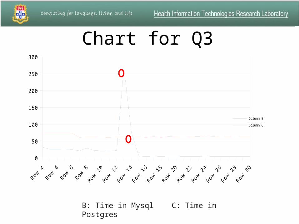
Chart for Q3
B: Time in Mysql C: Time in Postgres
0
50
100
150
200
250
300
Column B
Column C
• The time in Mysql is longer than the time in Postgres in most queries.
• For the queries which include more than two tables, it will take a very long time to execute in Mysql.
• But for the queries which only include one table, Mysql is usually faster than Postgres.
• But most queries include more than one table, so usually Postgres is more efficient than Mysql.
Conclusion
CLINIDAL and SQL
• We have finished Appendix question comparison of CLINIDAL and SQL results.
• For both data retrieval methods we are getting the same results.
• Kidney and Vasculitis are proving to be complex questions and we are doing CLINIDAL interface modifications at this stage.
Future Work
• SQL has limited capability to handle text based search.
• Comparison of CLINIDAL results with SQL findings for text based research questions will give us better idea, and that is in process at the moment.
Thank You


