Introduction The Timoshenko systems in thermoelasticity The Timoshenko with heat conduction damping Concluding Remarks
Damping by heat conduction in the Timoshenkosystem: Fourier and Cattaneo are the same
Belkacem Said-Houari
KAUST University, Saudi Arabia
December 3, 2012
Joint works with:
Aslan Kasimov (KAUST)
B. Said-Houari Timoshenko System December 3, 2012 1 / 40

Introduction The Timoshenko systems in thermoelasticity The Timoshenko with heat conduction damping Concluding Remarks
Table of contents
1 IntroductionThe Fourier lawThe Cattaneo lawSingle-phase-lagging model
2 The Timoshenko systems in thermoelasticityThe initial boundary value problemThe Cauchy problem
The coupling with the Fourier lawThe coupling with the Cattaneo law
3 The Timoshenko with heat conduction dampingThe Cattaneo modelThe energy method in the Fourier spaceThe Fourier model
4 Concluding Remarks
B. Said-Houari Timoshenko System December 3, 2012 2 / 40

Introduction The Timoshenko systems in thermoelasticity The Timoshenko with heat conduction damping Concluding Remarks
The Fourier law
In 1807, the French mathematical physicist Joseph Fourier proposed aconstitutive relation of the heat flux of the form
q(x , t) = −κ∇θ(x , t), (1)
where x stands for the material point, t is the time, q is the heat flux, θis the temperature, ∇ is the gradient operator and κ is the thermalconductivity of the material, which is a thermodynamic state property.Equation (1) together with the energy equation of the heat conduction
ρθt + %divq = 0 (2)
yields the classical heat transport equation (of parabolic type)
ρθt − κ%∆θ = 0, (3)
that allows an infinite speed for thermal signals.B. Said-Houari Timoshenko System December 3, 2012 3 / 40

Introduction The Timoshenko systems in thermoelasticity The Timoshenko with heat conduction damping Concluding Remarks
The Cattaneo law
To overcome the drawback in the Fourie law, a number of modifications ofthe basic assumption on the relation between the heat flux and thetemperature have been made, such as: Cattaneo law, Gurtin & Pipkintheory, Jeffreys law, Green & Naghdi theory and others. The commonfeature of these theories is that all lead to hyperbolic differential equationand permit transmission of heat flow as thermal waves at finite speed.The Cattaneo law
τqt+q + κ∇θ = 0, (τ > 0, relatively small) (4)
was proposed by Cattaneo in 1948. It is perhaps the most obvious, themost widely accepted and simplest generalization of Fourier’s law thatgives rise to a finite speed of propagation of heat.
B. Said-Houari Timoshenko System December 3, 2012 4 / 40
Introduction The Timoshenko systems in thermoelasticity The Timoshenko with heat conduction damping Concluding Remarks
The Cattaneo law
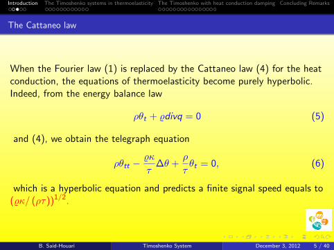
When the Fourier law (1) is replaced by the Cattaneo law (4) for the heatconduction, the equations of thermoelasticity become purely hyperbolic.Indeed, from the energy balance law
ρθt + %divq = 0 (5)
and (4), we obtain the telegraph equation
ρθtt −%κ
τ∆θ +
ρ
τθt = 0, (6)
which is a hyperbolic equation and predicts a finite signal speed equals to(%κ/ (ρτ))1/2.
B. Said-Houari Timoshenko System December 3, 2012 5 / 40

Introduction The Timoshenko systems in thermoelasticity The Timoshenko with heat conduction damping Concluding Remarks
Single-phase-lagging model
Note that the Cattaneo constitutive relation (4) is actually a first-orderapproximation of a more general constitutive relation (single-phase-laggingmodel).
q(x , t + τ) = −κ∇θ(x , t). (7)
The relation (7) states that the temperature gradient established at apoint x at time t gives rise to a heat flux vector at x at a later time t + τ .The delay time τ is interpreted as the relaxation time due to thefast-transient effects of thermal inertia (or small-scale effects of heattransport in time) and is called the phase-lag of the heat flux.It has been confirmed by many experiments that the Cattaneo lawgenerates a more accurate prediction than the classical Fourier law.However, some studies show that the Cattaneo constitutive relation hasonly taken account of the fast-transient effects, but not themicro-structural interactions.
B. Said-Houari Timoshenko System December 3, 2012 6 / 40

Introduction The Timoshenko systems in thermoelasticity The Timoshenko with heat conduction damping Concluding Remarks
The coupling of the heat conduction with elasticity
Racke (2002) has shown that the norm of the difference
between the solution U = (u, ut , θ, q) of the classical thermoelastic systemutt − αuxx + βθx = 0,
θt + qx + δutx = 0,
q + κθx = 0,
and the solution U =(u, ut , θ, q
)of the second sound thermoelastic
model utt − αuxx + βθx = 0,
θt + qx + δutx = 0,
τ qt + q + κθx = 0,
can be estimated as∥∥∥U(t, x)− U(t, x)
∥∥∥2≤ Cτ2. This last estimate
means that the difference will go to zero as τ → 0.B. Said-Houari Timoshenko System December 3, 2012 7 / 40

Introduction The Timoshenko systems in thermoelasticity The Timoshenko with heat conduction damping Concluding Remarks
Coupling of the heat conduction with the Timoshenko system
The Timoshenko system consists of a coupled system of two waveequations describing the transverse vibration of a beam and it ignoresdamping effects of any nature. Specifically, Timoshenko derived thefollowing system{
ρϕtt = (K (ϕx − ψ))x , in (0, L)× (0,+∞),
Iρψtt = (EIψx)x + K (ϕx − ψ)), in (0, L)× (0,+∞),(8)
where t is time, x is the coordinate along the beam length. The functionϕ = ϕ(t, x) is the transverse displacement of the beam from anequilibrium state and ψ = ψ(t, x) is the rotation angle of the filament ofthe beam. The coefficients ρ, Iρ,E , I and K are, respectively, the density,the polar moment of inertia of a cross section, Young’s modulus ofelasticity, the moment of inertia of a cross section, and the shear modulus.
B. Said-Houari Timoshenko System December 3, 2012 8 / 40

Introduction The Timoshenko systems in thermoelasticity The Timoshenko with heat conduction damping Concluding Remarks
Some Results
Rivera and Racke (2002)→ Heat conduction through Fourier’s lawρ1ϕtt − σ(ϕx , ψ)x = 0, in (0, L)× (0,+∞),
ρ2ψtt − bψxx + k (ϕx + ψ) + γθx = 0, in (0, L)× (0,+∞),
ρ3θt − kθxx + γψtx = 0 in (0, L)× (0,+∞)
→ Exponential decay results for the linearized system and a non exponentialstability result for the case of different wave speeds.
Fernandez Sare and Racke (2009)→ Heat conduction through Cattaneo’slaw
ρ1ϕtt − K (ϕx + ψ)x = 0ρ2ψtt − bψxx + K (ϕx + ψ) + γθx = 0ρ3θt + κqx + γψtx = 0τ0qt + δq + κθx = 0,
(9)
→ No exponential decay even if the wave speeds are equal.
And additional damping of the form
∫ ∞0
g(t − s)ψxx(s)ds in the left-hand
side of (9) is not enough to stabilize the system exponentially.B. Said-Houari Timoshenko System December 3, 2012 9 / 40

Introduction The Timoshenko systems in thermoelasticity The Timoshenko with heat conduction damping Concluding Remarks
The Cauchy problem (only few results)
Ide, Haramoto & Kawashima (2008) investigated the problemϕtt (t, x)− (ϕx − ψ)x (t, x) = 0, (t, x) ∈ R+ × R,
ψtt (t, x)−a2ψxx (t, x)− (ϕx − ψ) (t, x) +λψt (t, x) = 0, (t, x) ∈ R+ × R,
(ϕ,ϕt , ψ, ψt) (0, x) = (ϕ0, ϕ1, ψ0, ψ1) , x ∈ R,(10)
where a and λ are positive constants. They proved that if a = 1, then solutions of(10) decay as∥∥∂kxU (t)
∥∥2≤ C (1 + t)−1/4−k/2 ‖U0‖1 + Ce−ct
∥∥∂kxU0
∥∥2, (11)
where U = (ϕx − ψ,ϕt , aψx , ψt)T . If on the other hand, a 6= 1, then decay
property of system (10) is of regularity-loss type and solutions decay as∥∥∂kxU (t)∥∥
2≤ C (1 + t)−1/4−k/2 ‖U0‖1 + C (1 + t)−l/2 ∥∥∂k+l
x U0
∥∥2. (12)
The parameters k and l in (11) and (12) are non-negative integers, and C and c
are positive constants.B. Said-Houari Timoshenko System December 3, 2012 10 / 40

Introduction The Timoshenko systems in thermoelasticity The Timoshenko with heat conduction damping Concluding Remarks
Racke & Said-Houari (2011) analyzed the semilinear problem
ϕtt − (ϕx − ψ)x = 0, (t, x) ∈ R+ × R,
ψtt − a2ψxx − (ϕx − ψ) +λψt = f (ψ) , (t, x) ∈ R+ × R,
(ϕ,ϕt , ψ, ψt) (0, x) = (ϕ0, ϕ1, ψ0, ψ1) , x ∈ R,
(13)
where f (ψ (t, x)) = |ψ (t, x)|p with p > 1. For the linear case (i.e. f = 0), they
improved the decay results obtained in (11) so that, for initial data
U0 ∈ Hs (R) ∩ L1,γ (R) with a suitably large s and γ ∈ [0, 1], solutions decay
faster than those given in (11) and (12). Further, we analyzed the asymptotic
behavior of the semilinear problem (13) with the power type nonlinearity |ψ|p
with p > 12.
B. Said-Houari Timoshenko System December 3, 2012 11 / 40

Introduction The Timoshenko systems in thermoelasticity The Timoshenko with heat conduction damping Concluding Remarks
The Cauchy problem: The coupling with the Fourier law
Said-Houari & Kasimov (2012)
We considered the Fourier-Timoshenko system:ϕtt − (ϕx − ψ)x = 0,
ψtt − a2ψxx − (ϕx − ψ) + λψt + βθx = 0,
θt − θxx + βψtx = 0,
(14)
where t ∈ (0,∞) denotes the time variable and x ∈ R is the space variable, thefunctions ϕ and ψ denote the displacements of the elastic material, the function θis the temperature difference and a, λ and β are certain positive constants.Initial conditions are of the following form,{
ϕ(., 0) = ϕ0(x), ϕt(., 0) = ϕ1(x), ψ(., 0) = ψ0(x),
ψt(., 0) = ψ1(x), θ(., 0) = θ0 (x) .(15)
B. Said-Houari Timoshenko System December 3, 2012 12 / 40

Introduction The Timoshenko systems in thermoelasticity The Timoshenko with heat conduction damping Concluding Remarks
Let us first write system (73)-(74) as a first order (in time) system of the form{Ut + AUx + LU = BUxx ,
U (x, 0) = U0.(16)
where A, L, B are matrices and U is a solution vector identified below. To obtain system (16), we introduce the followingvariables:
v = ϕx − ψ, u = ϕt , z = aψx , y = ψt .
Consequently, system (73) can be rewritten into the following first order system of hyperbolic-parabolic type
vt − ux + y = 0,
ut − vx = 0,
zt − ayx = 0,
yt − azx − v + λy + βθx = 0,
θt − θxx + βyx = 0,
(17)
System (75) is equivalent to system (16) with
U =
vuzyθ
, A =
0 −1 0 0 0−1 0 0 0 00 0 0 −a 00 0 −a 0 β0 0 0 β 0
, L =
0 0 0 1 00 0 0 0 00 0 0 0 0−1 0 0 λ 00 0 0 0 0
,
B=
0 0 0 0 00 0 0 0 00 0 0 0 00 0 0 0 00 0 0 0 −1
.B. Said-Houari Timoshenko System December 3, 2012 13 / 40

Introduction The Timoshenko systems in thermoelasticity The Timoshenko with heat conduction damping Concluding Remarks
Fourier law: U0 ∈ Hs(R) ∩ L1(R)
Theorem 1
Let s be a nonnegative integer and assume that U0 ∈ Hs(R) ∩ L1(R). Then thesolution U of problem (16) satisfies the following decay estimates:
When a = 1,∥∥∂kxU (t)∥∥
2≤ C (1 + t)−1/4−k/2 ‖U0‖L1 + Ce−ct
∥∥∂kxU0
∥∥2. (18)
When a 6= 1,∥∥∂kxU (t)∥∥
2≤ C (1 + t)−1/4−k/2 ‖U0‖L1 + C (1 + t)−l/2 ∥∥∂k+l
x U0
∥∥2, (19)
where k and l are non-negative integers satisfying k + l ≤ s and C , c are twopositive constants.
B. Said-Houari Timoshenko System December 3, 2012 14 / 40
Introduction The Timoshenko systems in thermoelasticity The Timoshenko with heat conduction damping Concluding Remarks
The Fourier law: U0 ∈ Hs(R) ∩ L1,γ(R)
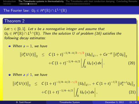
Theorem 2
Let γ ∈ [0, 1]. Let s be a nonnegative integer and assume thatU0 ∈ Hs(R) ∩ L1,γ(R). Then the solution U of problem (16) satisfies thefollowing decay estimates:
When a = 1, we have∥∥∂kxU (t)∥∥
2≤ C (1 + t)−1/4−k/2−γ/2 ‖U0‖L1,γ + Ce−ct
∥∥∂kxU0
∥∥2
+C (1 + t)−1/4−k/2
∣∣∣∣∫RU0 (x) dx
∣∣∣∣ . (20)
When a 6= 1, we have∥∥∂kxU (t)∥∥
2≤ C (1 + t)−1/4−k/2−γ/2 ‖U0‖L1,γ + C (1 + t)−l/2 ∥∥∂k+l
x U0
∥∥2
+C (1 + t)−1/4−k/2
∣∣∣∣∫RU0 (x) dx
∣∣∣∣ , (21)
where k and l are non-negative integers satisfying k + l ≤ s and C , c are twopositive constants.
B. Said-Houari Timoshenko System December 3, 2012 15 / 40

Introduction The Timoshenko systems in thermoelasticity The Timoshenko with heat conduction damping Concluding Remarks
The Cauchy problem: The coupling with the Cattaneo law
The second problem we investigate in the present work is the followingTimoshenko system in thermoelasticity of second sound
ϕtt − (ϕx − ψ)x = 0,
ψtt − a2ψxx − (ϕx − ψ) + βθx + λψt = 0,
θt + κqx + βψtx = 0,
τqt + δq + κθx = 0.
(22)
where t ∈ (0,∞) and x ∈ R and γ, τ, δ, κ, λ and β are positive constants and thefollowing initial conditions are assumed,{
ϕ(., 0) = ϕ0(x), ϕt(., 0) = ϕ1(x), ψ(., 0) = ψ0(x),
ψt(., 0) = ψ1(x), θ(., 0) = θ0 (x) , q(., 0) = q0 (x) .(23)
B. Said-Houari Timoshenko System December 3, 2012 16 / 40
Introduction The Timoshenko systems in thermoelasticity The Timoshenko with heat conduction damping Concluding Remarks
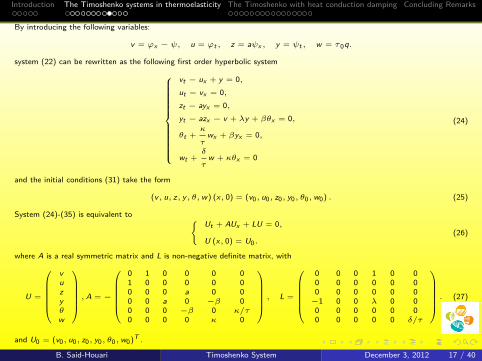
By introducing the following variables:
v = ϕx − ψ, u = ϕt , z = aψx , y = ψt , w = τ0q.
system (22) can be rewritten as the following first order hyperbolic system
vt − ux + y = 0,
ut − vx = 0,
zt − ayx = 0,
yt − azx − v + λy + βθx = 0,
θt +κ
τwx + βyx = 0,
wt +δ
τw + κθx = 0
(24)
and the initial conditions (31) take the form
(v, u, z, y, θ,w) (x, 0) = (v0, u0, z0, y0, θ0,w0) . (25)
System (24)-(35) is equivalent to {Ut + AUx + LU = 0,
U (x, 0) = U0.(26)
where A is a real symmetric matrix and L is non-negative definite matrix, with
U =
vuzyθw
, A = −
0 1 0 0 0 01 0 0 0 0 00 0 0 a 0 00 0 a 0 −β 00 0 0 −β 0 κ/τ0 0 0 0 κ 0
, L =
0 0 0 1 0 00 0 0 0 0 00 0 0 0 0 0−1 0 0 λ 0 00 0 0 0 0 00 0 0 0 0 δ/τ
. (27)
and U0 = (v0, u0, z0, y0, θ0,w0)T .
B. Said-Houari Timoshenko System December 3, 2012 17 / 40

Introduction The Timoshenko systems in thermoelasticity The Timoshenko with heat conduction damping Concluding Remarks
System (26) can be seen as a particular case of a general hyperbolic system ofbalance laws. We point out that Shizuta & Kawashima introduced the so-calledalgebraic condition (SK), namely
(SK) ∀ξ ∈ R−{0} , Ker(L) ∩ {eigenvectors of (ξA)} = {0},
which is satisfied in many examples and sufficient to establish a general result ofglobal existence for small perturbations of constant-equilibrium state. Our system(26) satisfies the condition (SK), but the general theory on the dissipativestructure established by Shizuta & Kawashima (1985) is not applicable since thematrices A and L are not real symmetric.Beauchard & Zuazua (2011) have recently shown that the condition (SK) isequivalent to the classical Kalman rank condition in control theory for the pair(A, L), that is
rk[L, A(iξ)L, ..., A(iξ)N−1L] = N,
where A(iξ) = iξA is an N × N matrix.
B. Said-Houari Timoshenko System December 3, 2012 18 / 40
Introduction The Timoshenko systems in thermoelasticity The Timoshenko with heat conduction damping Concluding Remarks
The Cattaneo law: Decay results
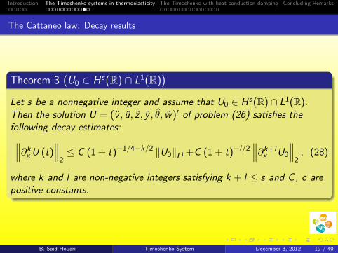
Theorem 3 (U0 ∈ H s(R) ∩ L1(R))
Let s be a nonnegative integer and assume that U0 ∈ Hs(R) ∩ L1(R).Then the solution U = (v , u, z , y , θ, w)′ of problem (26) satisfies thefollowing decay estimates:∥∥∥∂kxU (t)
∥∥∥2≤ C (1 + t)−1/4−k/2 ‖U0‖L1 +C (1 + t)−l/2
∥∥∥∂k+lx U0
∥∥∥2, (28)
where k and l are non-negative integers satisfying k + l ≤ s and C , c arepositive constants.
B. Said-Houari Timoshenko System December 3, 2012 19 / 40

Introduction The Timoshenko systems in thermoelasticity The Timoshenko with heat conduction damping Concluding Remarks
Theorem 4 (U0 ∈ H s(R) ∩ L1,γ(R))
Let γ ∈ [0, 1], let s be a nonnegative integer, and assume thatU0 ∈ Hs(R)∩ L1,γ(R). Then the solution U = (v , u, z , y , θ, w)′ of problem(26) satisfies the following decay estimates:∥∥∥∂kxU (t)
∥∥∥2≤ C (1 + t)−1/4−k/2−γ/2 ‖U0‖L1,γ + C (1 + t)−l/2
∥∥∥∂k+lx U0
∥∥∥2
+C (1 + t)−1/4−k/2
∣∣∣∣∫RU0 (x) dx
∣∣∣∣ , (29)
where k and l are non-negative integers satisfying k + l ≤ s and C and care two positive constants.
B. Said-Houari Timoshenko System December 3, 2012 20 / 40
Introduction The Timoshenko systems in thermoelasticity The Timoshenko with heat conduction damping Concluding Remarks
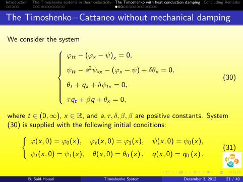
The Timoshenko−Cattaneo without mechanical damping
We consider the system
ϕtt − (ϕx − ψ)x = 0,
ψtt − a2ψxx − (ϕx − ψ) + δθx = 0,
θt + qx + δψtx = 0,
τqt + βq + θx = 0,
(30)
where t ∈ (0,∞), x ∈ R, and a, τ, δ, β, β are positive constants. System(30) is supplied with the following initial conditions:{
ϕ(x , 0) = ϕ0(x), ϕt(x , 0) = ϕ1(x), ψ(x , 0) = ψ0(x),
ψt(x , 0) = ψ1(x), θ(x , 0) = θ0 (x) , q(x , 0) = q0 (x) .(31)
B. Said-Houari Timoshenko System December 3, 2012 21 / 40

Introduction The Timoshenko systems in thermoelasticity The Timoshenko with heat conduction damping Concluding Remarks
To rewrite the system as a first-order system, we define new variables, as follows:
v = ϕx − ψ, u = ϕt , z = aψx , y = ψt , w = q. (32)
Then, (30) takes the form:
vt − ux + y = 0,
ut − vx = 0,
zt − ayx = 0,
yt − azx − v + δθx = 0,
θt + wx + δyx = 0,
wt +β
τw +
1
τθx = 0
(33)
and, if we denoteU(x , t) = (v , u, z , y , θ,w)T , (34)
the initial conditions can then be written as
U(x , 0) = U0(x) = (v0, u0, z0, y0, θ0,w0)T , (35)
where v0 = ϕ0,x − ψ0, u0 = ψ1, z0 = aψ0,x , y0 = ψ1, w0 = q0.
B. Said-Houari Timoshenko System December 3, 2012 22 / 40

Introduction The Timoshenko systems in thermoelasticity The Timoshenko with heat conduction damping Concluding Remarks
Theorem 5 (Cattaneo model τ 6= 0)
Let s be a nonnegative integer and let α = (τ − 1)(1− a2
)− τδ2.
Assume that U0 ∈ Hs(R) ∩ L1(R). Then, the solution, U, of problem (33)satisfies the following decay estimates:
if α = 0,∥∥∥∂kxU (t)∥∥∥
2≤ C (1 + t)−1/12−k/6 ‖U0‖1 + Ce−ct
∥∥∥∂kxU0
∥∥∥2
; (36)
if α 6= 0,∥∥∥∂kxU (t)∥∥∥
2≤ C (1 + t)−1/12−k/6 ‖U0‖1 + C (1 + t)−l/6
∥∥∥∂k+lx U0
∥∥∥2,
(37)
where k and l are non-negative integers satisfying k + l ≤ s and C and care two positive constants.
B. Said-Houari Timoshenko System December 3, 2012 23 / 40

Introduction The Timoshenko systems in thermoelasticity The Timoshenko with heat conduction damping Concluding Remarks
Taking the Fourier transform of (33), we obtain the following ODE system:
vt − iξu + y = 0, (38a)
ut − iξv = 0, (38b)
zt − aiξy = 0, (38c)
yt − aiξz − v + δiξθ = 0, (38d)
θt + iξw + δiξy = 0, (38e)
wt +β
τw +
1
τiξθ = 0, (38f)
together with initial data, written in terms of the solution vector, U (ξ, t) =(v, u, z, y, θ, w
)T, as
U(ξ, 0) = U0(ξ). (39)
Proposition 1
Let U (ξ, t) be a solution of (38)-(39) and α = (τ − 1)(
1− a2)− τδ2. Then, there exist two positive constants, C and c,
such that, for all t ≥ 0 :
∣∣∣U (ξ, t)∣∣∣2 ≤ C
∣∣∣U (ξ, 0)∣∣∣2 e−cρ1(ξ)
, ρ1 (ξ) =ξ6(
1 + ξ2)3, if α = 0, (40)
∣∣∣U (ξ, t)∣∣∣2 ≤ C
∣∣∣U (ξ, 0)∣∣∣2 e−cρ2(ξ)
, ρ2 (ξ) =ξ6(
1 + ξ2)6, if α 6= 0. (41)
B. Said-Houari Timoshenko System December 3, 2012 24 / 40

Introduction The Timoshenko systems in thermoelasticity The Timoshenko with heat conduction damping Concluding Remarks
Lemma 6
Define the following energy functional:
E (t) =1
2(|v |2 + |u|2 + |z |2 + |y |2 + |θ|2 + τ |w |2). (42)
Then,
c1
∣∣∣U (ξ, t)∣∣∣2 ≤ E (ξ, t) ≤ c2
∣∣∣U (ξ, t)∣∣∣2 , (43)
where c1 = min (1/2, τ/2) and c2 = max (1/2, τ/2) , and
d
dtE (t) = −βτ |w |2, ∀t ≥ 0. (44)
B. Said-Houari Timoshenko System December 3, 2012 25 / 40

Introduction The Timoshenko systems in thermoelasticity The Timoshenko with heat conduction damping Concluding Remarks
In the following lemma, we show a dissipative term of |v |2.
Lemma 7
The functional
G (t) = Re
[−τaz∗u +
(τ +
1
δ2− a2
δ2
)δθ∗u − τ v y∗
]+
1− a2
δRe (−τ v∗w)
(45)satisfies
d
dtG (t) + τ |v |2 − τ |y |2 =
1− a2
δβRe (w v∗) +
1− a2
δRe (τ w∗y)
+αRe (iξy u∗) +α
δRe (iξw u∗) , (46)
whereα = (τ − 1)
(1− a2
)− τδ2. (47)
B. Said-Houari Timoshenko System December 3, 2012 26 / 40

Introduction The Timoshenko systems in thermoelasticity The Timoshenko with heat conduction damping Concluding Remarks
Lemma 8
Let K (t) be defined by
K (t) = Re(iξu∗v + aiξ¯zy − δaτ iξz∗w
). (48)
Then, for any ε1, ε2 > 0,
d
dtK (t) + (1− ε1) ξ2 |u|2 +
(a2 − ε2
)ξ2 |z |2
≤ C (ε1, ε2)(1 + ξ2
) (|v |2 + |y |2
)+ C (ε2)
(1 + ξ2
)|w |2 . (49)
B. Said-Houari Timoshenko System December 3, 2012 27 / 40

Introduction The Timoshenko systems in thermoelasticity The Timoshenko with heat conduction damping Concluding Remarks
Lemma 9
The following inequalities hold true:
d
dtRe(iξw∗θ
)+
(1
τ− ε3
)ξ2|θ|2 ≤ C
(ε3, ε
′3
) (1 + ξ2
)|w |2+ε′3
ξ4
1 + ξ2|y |2
(50)and
d
dtRe(iξθ∗y
)+ (δ − ε4) ξ2 |y |2 ≤ C
(ε′4) (
1 + ξ2)|θ|2 + ε′4
ξ4
1 + ξ2|z |2
+ε′4ξ2 |v |2 + C (ε4) ξ2 |w |2 , (51)
where ε3, ε′3, ε4, and ε′4 are arbitrary positive constants.
B. Said-Houari Timoshenko System December 3, 2012 28 / 40

Introduction The Timoshenko systems in thermoelasticity The Timoshenko with heat conduction damping Concluding Remarks
Proof of Proposition 1
To prove Proposition 1, we consider the two cases, α = 0 and α 6= 0, separately.Case 1. α = 0.
In this case, (46) takes the formdG (t)
dt+ (τ − ε0) |v|2 ≤ C (ε0)
(|w|2 + |y|2
). (52)
Define the functional
L1 (t) =ξ2
1 + ξ2
{γ0ξ
2G (ξ, t) + γ1ξ2
1 + ξ2K (ξ, t) + γ4Re
(iξθ∗ y
)}
+γ3Re(iξw∗θ
)+ N
(1 + ξ
2)E (ξ, t) , (53)
where N, γ0, ..., γ4 are positive constants to be fixed later. Taking the derivative of L (ξ, t) with respect to t and using (52),(49), (51, and (50), we get Consequently, we deduce that there exists a positive constant, η > 0, such that
d
dtL1 (t) + ηQ1 (t) ≤ 0, ∀t ≥ 0, (54)
where
Q1 (t) =ξ4
1 + ξ2|v|2 +
ξ4
1 + ξ2|y|2 +
ξ6(1 + ξ2
)2
(|u|2 + |z|2
)+ ξ
2|θ|2 +(
1 + ξ2)|w|2 . (55)
It is not difficult to see now that, for all t ≥ 0 and for all ξ ∈ R, we have
Q1 (t) ≥ξ6(
1 + ξ2)2
(|v|2 + |y|2 + |u|2 + |z|2 + |θ|2 + |w|2
)
=ξ6(
1 + ξ2)2
∣∣∣U (ξ, t)∣∣∣2 . (56)
B. Said-Houari Timoshenko System December 3, 2012 29 / 40

Introduction The Timoshenko systems in thermoelasticity The Timoshenko with heat conduction damping Concluding Remarks
On the other hand we can show that
β1
(1 + ξ
2)E (t) ≤ L1 (t) ≤ β2
(1 + ξ
2)E (t) . (57)
Combining (43), (54), (56), and (57), we deduce that there exists a positive constant, η1 > 0, such that for all t ≥ 0, we have
d
dtL1 (t) ≤ −η1
ξ6(1 + ξ2
)3L1 (t) . (58)
Integrating (58) over t and using once again (43) and (57), we deduce (40).
Case 2. α 6= 0.
In this case, the two last terms on the right-hand side of (46) can be estimated as
αRe(iξy u∗
)+α
δRe(iξw u∗
)≤ ε′0
ξ2
1 + ξ2|u|2 + C
(ε′0
) (1 + ξ
2) (|y|2 + |w|2
). (59)
Inserting (59) into (46) and applying Young’s inequality as before, we find that (52) takes the form
dG (t)
dt+ (τ − ε0) |v|2 ≤ C
(ε′0, ε0
) (1 + ξ
2) (|w|2 + |y|2
)+ ε′0
ξ2
1 + ξ2|u|2 . (60)
Now, we define
L2 (t) =ξ2(
1 + ξ2)2
{λ0
ξ2
1 + ξ2G (ξ, t) + λ1
ξ2(1 + ξ2
)2K (ξ, t) + λ4Re
(iξθ∗ y
)}
+λ3Re(iξw∗θ
)+ M
(1 + ξ
2)2
E (ξ, t) , (61)
where M, εj , ε′d , and λj , with j = 1, ..., 4 and d = 0, 3, 4, are positive constants to be fixed later.
B. Said-Houari Timoshenko System December 3, 2012 30 / 40
Introduction The Timoshenko systems in thermoelasticity The Timoshenko with heat conduction damping Concluding Remarks
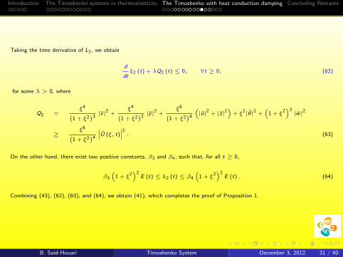
Taking the time derivative of L2, we obtain
d
dtL2 (t) + λQ2 (t) ≤ 0, ∀t ≥ 0, (62)
for some λ > 0, where
Q2 =ξ4(
1 + ξ2)3|v|2 +
ξ4(1 + ξ2
)2|y|2 +
ξ6(1 + ξ2
)4
(|u|2 + |z|2
)+ ξ
2|θ|2 +(
1 + ξ2)2|w|2
≥ξ6(
1 + ξ2)4
∣∣∣U (ξ, t)∣∣∣2 . (63)
On the other hand, there exist two positive constants, β3 and β4, such that, for all t ≥ 0,
β3
(1 + ξ
2)2
E (t) ≤ L2 (t) ≤ β4
(1 + ξ
2)2
E (t) . (64)
Combining (43), (62), (63), and (64), we obtain (41), which completes the proof of Proposition 1.
B. Said-Houari Timoshenko System December 3, 2012 31 / 40

Introduction The Timoshenko systems in thermoelasticity The Timoshenko with heat conduction damping Concluding Remarks
Proof of Theorem 5
The proof is based on the pointwise estimates in Proposition 1.First, let us assume that α = 0. Then, ρ1(ξ) ≥ 1
8ξ6, for |ξ| ≤ 1,
ρ1(ξ) ≥ 18, for |ξ| ≥ 1.
(65)
Applying the Plancherel theorem and making use of the inequality in (40), we obtain∥∥∥∂kx U (t)∥∥∥2
2=
∫R|ξ|2k
∣∣∣U (ξ, t)∣∣∣2 dξ
≤ C
∫R|ξ|2k e−cρ1(ξ)t
∣∣∣U (ξ, 0)∣∣∣2 dξ
= C
∫|ξ|≤1
|ξ|2k e−cρ1(ξ)t∣∣∣U (ξ, 0)
∣∣∣2 dξ + C
∫|ξ|≥1
|ξ|2k e−cρ1(ξ)t∣∣∣U (ξ, 0)
∣∣∣2 dξ
= I1 + I2. (66)
That is, the integral is split into its low-frequency part, I1, and its high-frequency part, I2. For I1, we find, by using the firstinequality in (65), that
I1 ≤ C
∫|ξ|≤1
|ξ|2k e− 1
8ξ6t∣∣∣U (ξ, 0)
∣∣∣2 dξ ≤ C∥∥∥U0
∥∥∥2
∞
∫|ξ|≤1
|ξ|2k e− 1
8ξ6t
dξ. (67)
Then, using the inequality ∫ 1
0|ξ|2k e
− 18ξ6t
dξ ≤ (1 + t)−1/6−k/3,
we estimateI1 ≤ ‖U0‖
21 C (1 + t)−1/6−k/3
. (68)
B. Said-Houari Timoshenko System December 3, 2012 32 / 40

Introduction The Timoshenko systems in thermoelasticity The Timoshenko with heat conduction damping Concluding Remarks
For I2, using the second inequality in (65), we find
I2 ≤ C
∫|ξ|≥1
|ξ|2k e− 1
8t∣∣∣U (ξ, 0)
∣∣∣2 dξ ≤ Ce− 1
8t∥∥∥∂kx U0
∥∥∥2
2. (69)
Therefore, estimate (36) holds by adding (68) and (69). Now, we assume that α 6= 0. Then, ρ2(ξ) ≥ 164ξ6, for |ξ| ≤ 1,
ρ2(ξ) ≥ 164ξ−6, for |ξ| ≥ 1.
(70)
As before, using (41), we find that∥∥∥∂kx U (t)∥∥∥2
2≤ C
∫|ξ|≤1
|ξ|2k e−cρ2(ξ)t∣∣∣U (ξ, 0)
∣∣∣2 dξ + C
∫|ξ|≥1
|ξ|2k e−cρ2(ξ)t∣∣∣U (ξ, 0)
∣∣∣2 dξ
= J1 + J2.
The low-frequency part, J1, is estimated as I1 and results in
J1 ≤ ‖U0‖21 C (1 + t)−1/6−k/3
. (71)
The high-frequency part, J2, using the second inequality in (70), can be estimated as
J2 ≤ C
∫|ξ|≥1
|ξ|2k e− 1
64ξ−6t
∣∣∣U (ξ, 0)∣∣∣2 dξ.
Using the inequality
sup|ξ|≥1
{|ξ|−2l e−cξ−6t
}≤ C (1 + t)−l/3
,
we obtain
J2 ≤ C sup|ξ|≥1
{|ξ|−2l e−cξ−6t
}∫|ξ|≥1
|ξ|2(k+l)∣∣∣U (ξ, 0)
∣∣∣2 dξ
≤ C (1 + t)−l/3∥∥∥∂k+l
x U0
∥∥∥2
2. (72)
Combining the estimates of J1 and J2, estimate (37) is established. This completes the proof of Theorem 5.B. Said-Houari Timoshenko System December 3, 2012 33 / 40
Introduction The Timoshenko systems in thermoelasticity The Timoshenko with heat conduction damping Concluding Remarks
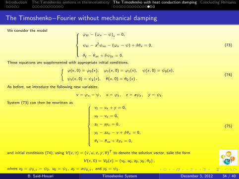
The Timoshenko−Fourier without mechanical damping
We consider the model ϕtt − (ϕx − ψ)x = 0,
ψtt − a2ψxx − (ϕx − ψ) + δθx = 0,
θt − θxx + δψtx = 0,
(73)
These equations are supplemented with appropriate initial conditions,{ϕ(x, 0) = ϕ0(x), ϕt (x, 0) = ϕ1(x), ψ(x, 0) = ψ0(x),
ψt (x, 0) = ψ1(x), θ(x, 0) = θ0 (x) .(74)
As before, we introduce the following new variables:
v = ϕx − ψ, u = ϕt , z = aψx , y = ψt .
System (73) can then be rewritten as
vt − ux + y = 0,
ut − vx = 0,
zt − ayx = 0,
yt − azx − v + δθx = 0,
θt − θxx + δyx = 0,
(75)
and initial conditions (74), using V (x, t) = (v, u, z, y, θ)T to denote the solution vector, take the form
V (x, 0) = V0(x) = (v0, u0, z0, y0, θ0) , (76)
where v0 = ϕ0,x − ψ0, u0 = ψ1, z0 = aψ0,x , and y0 = ψ1.
B. Said-Houari Timoshenko System December 3, 2012 34 / 40

Introduction The Timoshenko systems in thermoelasticity The Timoshenko with heat conduction damping Concluding Remarks
Theorem 10
Let s be a nonnegative integer and assume that V0 ∈ Hs(R) ∩ L1(R). Then, thesolution, V , of problem (75)-(76) satisfies the following decay estimates:
when a = 1,∥∥∂kxV (t)∥∥
2≤ C (1 + t)−1/12−k/6 ‖V0‖1 + Ce−ct
∥∥∂kxV0
∥∥2
; (77)
when a 6= 1,∥∥∂kxV (t)∥∥
2≤ C (1 + t)−1/12−k/6 ‖V0‖1 + C (1 + t)−l/2 ∥∥∂k+l
x V0
∥∥2, (78)
where k and l are non-negative integers satisfying k + l ≤ s, and C and c are twopositive constants.
B. Said-Houari Timoshenko System December 3, 2012 35 / 40

Introduction The Timoshenko systems in thermoelasticity The Timoshenko with heat conduction damping Concluding Remarks
Taking the Fourier transform of (75), we obtain
vt − iξu + y = 0, (79a)
ut − iξv = 0, (79b)
zt − aiξy = 0, (79c)
yt − aiξz − v + δiξθ = 0, (79d)
θt + ξ2θ + δiξy = 0, (79e)
with the initial data written in terms of V (ξ, t) = (v, u, z, y, θ)T :
V (ξ, 0) = V0(ξ, 0) = (v0, u0, z0, y0, θ0)T . (80)
Proposition 2
Let V (ξ, t) be the solution of (79)-(80). Then, there exist two positive constants, C and c, such that, for all t ≥ 0, thefollowing estimates hold true:if a = 1, ∣∣∣V (ξ, t)
∣∣∣2 ≤ C∣∣∣V (ξ, 0)
∣∣∣2 e−c%1(ξ), %1 (ξ) =
ξ6(1 + ξ2
) (1 + ξ2 + ξ4
) ; (81)
if a 6= 1, ∣∣∣V (ξ, t)∣∣∣2 ≤ C
∣∣∣V (ξ, 0)∣∣∣2 e−c%2(ξ)
, %2 (ξ) =ξ6(
1 + ξ2)2 (1 + ξ2 + ξ4
) . (82)
B. Said-Houari Timoshenko System December 3, 2012 36 / 40

Introduction The Timoshenko systems in thermoelasticity The Timoshenko with heat conduction damping Concluding Remarks
We proved here that there is essentially no difference between theTimoshenko-Cattaneo model and the Timoshenko-Fourier model interms of decay rates and regularity assumptions on the initial data. Inthe regularity-loss case and in both systems, the decay rate isobtained only for low-order derivatives, but not for all derivatives upto order s. Indeed, for the Cattaneo model, we see from (37) that ourestimates can be obtained for all k satisfying0 ≤ k ≤ [s/2− 1/4] = s1. For the Fourier model, we find from (78)that our estimates hold for 0 ≤ k ≤ [3s/4− 1/8] = s2. We see thats1 < s2 which is the only difference between the two models.
B. Said-Houari Timoshenko System December 3, 2012 37 / 40

Introduction The Timoshenko systems in thermoelasticity The Timoshenko with heat conduction damping Concluding Remarks
By comparing our present result with other known results on thisproblem, we see that in bounded domains and for appropriateassumptions on the coefficients, the following models all lead to anexponential decay rate:
only linear mechanical damping ψt present as in (10).
only viscoelastic damping present, i.e.,∫ t
0g(s)ψxx(t − s)ds instead of
ψt in (10) with an exponentially decaying g(s));Fourier heat conduction with no mechanical damping.Cattaneo heat conduction with no mechanical damping.
However, this is not true for the Cauchy problem. Indeed, withfrictional damping as in (10), the decay rate of the L2-norm is(1 + t)−1/4 (Ide & Kawashima), with the viscoelastic damping, thedecay rate is (1 + t)−1/8 (Liu & Kawashima), whereas as we haveshown here, the decay rate with heat dissipation alone is (1 + t)−1/12.As we see, the heat dissipation is slowest of all. The fact that bothFourier and Cattaneo models lead to the same decay rate smears thedistinction between them that prior studies have highlighted.
B. Said-Houari Timoshenko System December 3, 2012 38 / 40

Introduction The Timoshenko systems in thermoelasticity The Timoshenko with heat conduction damping Concluding Remarks
As in Theorem 2, it can be shown that if one assumes that∫R U0(x)dx = 0, then the decay rate in Theorem 5 can be improved.
Nevertheless, the total decay rate is still polynomial. We recall thatthe assumption
∫R U0(x)dx = 0 is equivalent to U0(0) = 0. An
exponential decay rate can be obtained by assuming that U0(ξ) = 0for |ξ|2 ≤ α0, with some α0 > 0.
The decay rates can be further improved by assuming that the highermomenta of the initial data are zeros.
B. Said-Houari Timoshenko System December 3, 2012 39 / 40

Introduction The Timoshenko systems in thermoelasticity The Timoshenko with heat conduction damping Concluding Remarks
Thank you for your attention
B. Said-Houari Timoshenko System December 3, 2012 40 / 40


