
CVXMOD: Convex Optimization in Python
Jacob Mattingley
joint work with Stephen Boyd
Electrical Engineering Department, Stanford University
INFORMS, 10/12/08
CVXMOD
• convex optimization modeling layer, in Python
• completely open source, object-oriented toolchain
• form problems easily using basic set of atoms and composition rulesfrom convex analysis
• uses CVXOPT’s general nonlinear convex solver (Vandenberghe, Dahl2005)
• generate custom C for real-time embedded convex optimization
INFORMS, 10/12/08 1

Outline
• modeling languages and disciplined convex programming
• example: optimal execution
• real-time embedded optimization
• code generation
INFORMS, 10/12/08 2

History
• general purpose optimization modeling systems AMPL, GAMS (1970s),many others...
• systems for SDPs/LMIs (1990s): SDPSOL (Wu, Boyd),LMILAB (Gahinet, Nemirovsky), LMITOOL (El Ghaoui)
• YALMIP (Lofberg 2000–)
• automated convexity checking (Crusius PhD thesis 2002)
• disciplined convex programming (DCP) (Grant, Boyd, Ye 2004)
• CVX (Grant, Boyd, Ye 2005)
• CVXOPT (Dahl, Vandenberghe 2005)
• GGPLAB (Mutapcic, Koh, et al 2006)
INFORMS, 10/12/08 3
Determining convexity—two approaches
• user creates (almost any) model; system attempts to verify convexity
– hard problem– best effort– detect convexity with automatic differentiation and interval analysis
Orban, Fourer 2004 (Dr. AMPL), Nenov, Fylstra, Kolev 2004
• user creates model following a restricted set of rules that ensureconvexity
– model is convex by construction– seems more useful to us in engineering– user must have some understanding and skill– CVX, CVXMOD
INFORMS, 10/12/08 4
Disciplined convex programming
• convex-by-construction method
• expressions appearing in objective and constraints are formed from
– an extensible set of atoms (functions)– a small set of combination rules derived from convex analysis
• rule set is intentionally small; not “as many rules as possible”
• we’ve found it surprisingly versatile
INFORMS, 10/12/08 5

Example
‖Ax − b‖2
• made from variable x, parameters A and b, atom ‖ · ‖2
• expression Ax − b is affine in x
• composite expression ‖Ax − b‖2 is convex, positive, non-monotonic
– could use it in objective, minimize(‖Ax − b‖2)– could use it in constraint, ‖Ax − b‖2 ≤ 1
• represent in CVXMOD as norm2(A*x - b)
INFORMS, 10/12/08 6

Composition rules
• can combine atoms using valid composition rules, e.g.:
– a convex function of an affine function is convex– the negative of a convex function is concave– a convex, nondecreasing function of a convex function is convex– a concave, nondecreasing function of a concave function is concave
• for convex h, h(g1, . . . , gk) is recognized as convex if, for each i,
– gi is affine, or– gi is convex and h is nondecreasing in its ith arg, or– gi is concave and h is nonincreasing in its ith arg
• for concave h, h(g1, . . . , gk) is recognized as concave if, for each i,
– gi is affine, or– gi is convex and h is nonincreasing in ith arg, or– gi is concave and h is nondecreasing in ith arg
INFORMS, 10/12/08 7

Valid (recognized) examples
u, v, x, y are scalar variables; X is a symmetric 3 × 3 variable
• convex:
– norm2(A*x - y) + 0.1*norm1(x)
– maxeig(2*X - 4*eye(3))
• concave:
– min(1 + 2*u, 1 - max(2, v))
– sqrt(v) - 4.55*invpos(u - v)
INFORMS, 10/12/08 8

Rejected examples
u, v, x, y are scalar variables
• neither convex nor concave:
– square(x) - square(y)
– norm(A*x - y) - 0.1*norm(x, 1)
• rejected due to limited DCP ruleset:
– sqrt(sum(square(x))) (is convex; could use norm(x))
– norm(x) - 0.1*norm(x) (is convex; could use 0.9*norm(x))
INFORMS, 10/12/08 9
Problem transformation
• DCP makes automatic transformation to convex standard form easy
• based on epigraphical transformations
INFORMS, 10/12/08 10

Transformation example
variables x, y; parameters A, b
‖Ax − b‖∞ ≤ 3 log(y)
INFORMS, 10/12/08 11

Transformation example
variables x, y; parameters A, b
‖Ax − b‖∞ ≤ 3 log(y)
• introduce variable t1, to get
t1 = Ax − b
‖t1‖∞ ≤ 3 log(y)
INFORMS, 10/12/08 12

Transformation example
variables x, y; parameters A, b
‖Ax − b‖∞ ≤ 3 log(y)
• introduce t2, to get
t1 = Ax − b
t2 ≤ 3 log(y)
−t21 ≤ t1 ≤ t21
INFORMS, 10/12/08 13

Transformation example
variables x, y; parameters A, b
‖Ax − b‖∞ ≤ 3 log(y)
• lastly, introduce variable t3, to get
t1 = Ax − b
t2 ≤ 3t3
−t21 ≤ t1 ≤ t21
t3 ≤ log(y)
INFORMS, 10/12/08 14
Outline
• modeling languages and disciplined convex programming
• example: optimal execution
• real-time embedded optimization
• code generation
INFORMS, 10/12/08 15

Optimal execution
• execute a sell order for S shares over T time periods
• prices modeled as random walk, plus price decrease from current andprevious sales
• maximize expected revenue
• yields (convex) quadratic program
maximize pTs − sTQssubject to 0 ≤ s ≤ Smax
1Ts = S
• obvious initialization of sales: si = S/T , i = 1, . . . , T
INFORMS, 10/12/08 16

Specifying problem family in CVXMOD
optimal sell order execution
s = optvar('s', T)
S = param('S')
pbar = param('pbar')
prob = problem(maximize(tp(pbar)*s - quadform(s, Q)),
[0 <= s, s <= Smax, sum(s) == S])
(Q, Smax, T have previously defined numerical values)
• describes a problem family, parameterized by pbar, S
• every symbol (s, pbar, prob, ...) is a (manipulable) Python object
INFORMS, 10/12/08 17

Solving problem instance in CVXMOD
pbar.value = linspace(10, 12, 20)
S.value = 100 + 1000*rand()
prob.solve()
• prob now contains a problem instance
• prob.solve()
– transforms prob into standard form– calls CVXOPT’s solver– transforms solution back to original variables
• after solution, access value() of any cvxmod object(value(s), value(s <= Smax), quadform(s, Q), ...)
INFORMS, 10/12/08 18
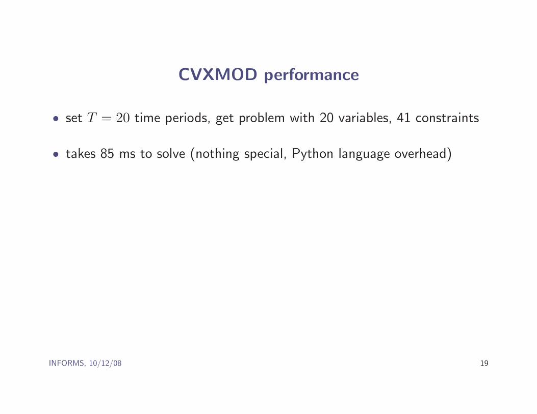
CVXMOD performance
• set T = 20 time periods, get problem with 20 variables, 41 constraints
• takes 85 ms to solve (nothing special, Python language overhead)
INFORMS, 10/12/08 19
Outline
• modeling languages and disciplined convex programming
• example: optimal execution
• real-time embedded optimization
• code generation
INFORMS, 10/12/08 20
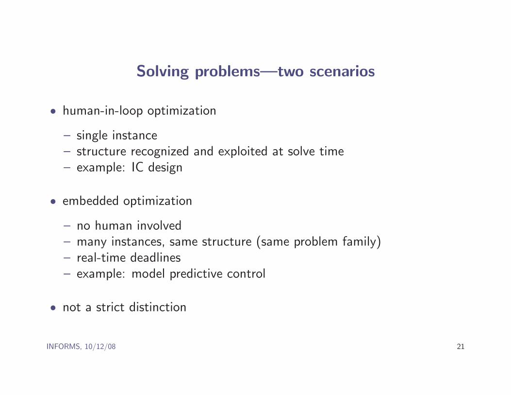
Solving problems—two scenarios
• human-in-loop optimization
– single instance– structure recognized and exploited at solve time– example: IC design
• embedded optimization
– no human involved– many instances, same structure (same problem family)– real-time deadlines– example: model predictive control
• not a strict distinction
INFORMS, 10/12/08 21

Embedded optimization
• compile time almost doesn’t matter
• detect and exploit structure once, at compile time
• solve time is critical: O(ms) or O(µs), even O(ns)
• relaxed accuracy requirements
• can exploit clever initializations (including warm start)
• currently done by custom code development
INFORMS, 10/12/08 22

Outline
• modeling languages and disciplined convex programming
• example: optimal execution
• real-time embedded optimization
• code generation
INFORMS, 10/12/08 23
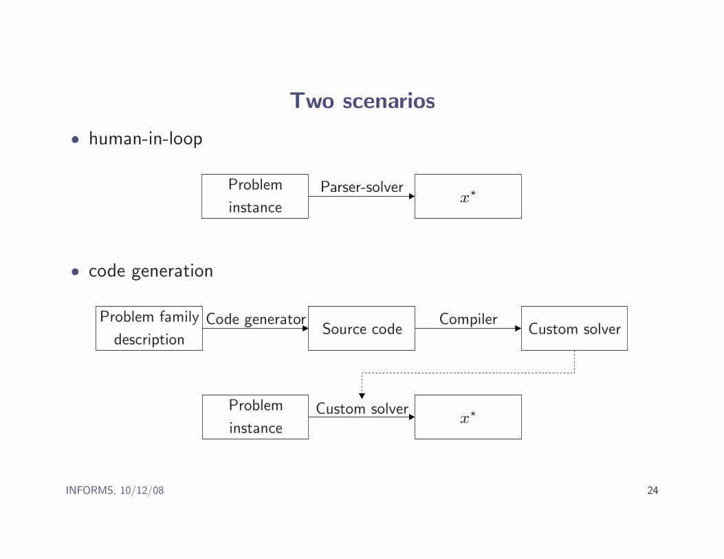
Two scenarios
• human-in-loop
Problem
instance
Parser-solverx
⋆
• code generation
Source codeCode generatorProblem family
description
Custom solver
Custom solverCompiler
Problem
instancex
⋆
INFORMS, 10/12/08 24

Code generation in CVXMOD
• preliminary implementation (not yet released)
• generates C source code from CVXMOD problem family specification
• solver uses simple primal barrier method
• at code generation time
– analyzes sparsity– determines memory arrangements
• search direction computation uses no libraries (faster) or CHOLMOD(smaller code)
INFORMS, 10/12/08 25
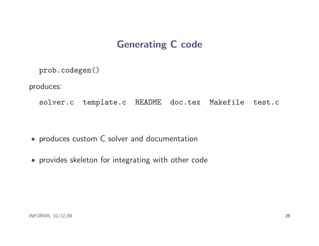
Generating C code
prob.codegen()
produces:
solver.c template.c README doc.tex Makefile test.c
• produces custom C solver and documentation
• provides skeleton for integrating with other code
INFORMS, 10/12/08 26
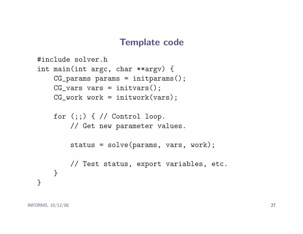
Template code
#include solver.h
int main(int argc, char **argv) {
CG_params params = initparams();
CG_vars vars = initvars();
CG_work work = initwork(vars);
for (;;) { // Control loop.
// Get new parameter values.
status = solve(params, vars, work);
// Test status, export variables, etc.
}
}
INFORMS, 10/12/08 27
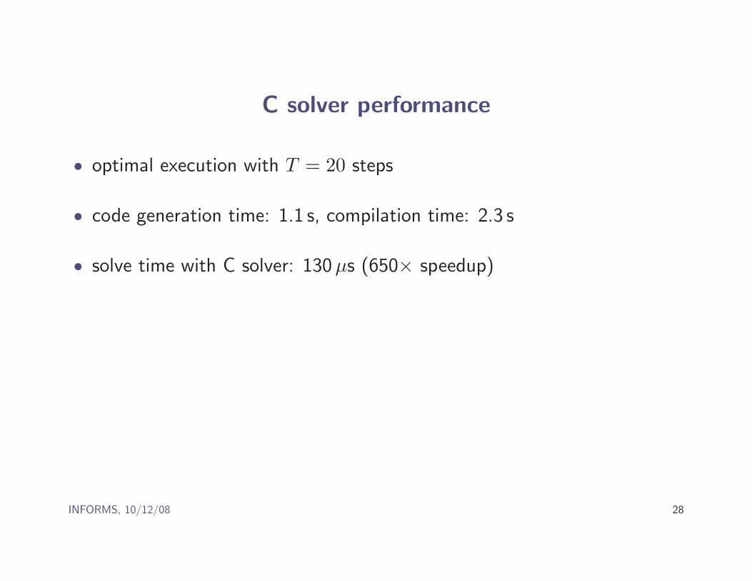
C solver performance
• optimal execution with T = 20 steps
• code generation time: 1.1 s, compilation time: 2.3 s
• solve time with C solver: 130 µs (650× speedup)
INFORMS, 10/12/08 28

Using CVXMOD
• prototype, test, simulate model in Python
• generate C solver source
• embed in application
INFORMS, 10/12/08 29

Summary
• CVXMOD as a modeling language using disciplined convexprogramming
• real-time embedded optimization (O(µs))
• CVXMOD as a code generator for real-time embedded optimization
INFORMS, 10/12/08 30


