
CURRENCY DEPRECIATION AND THE TRADE BALANCE:
AN ELASTICITY APPROACH AND TEST OF THE MARSHALL-LERNER
CONDITION FOR BILATERAL TRADE BETWEEN THE US AND THE G-7
by
Taggert J. Brooks
A Dissertation Submitted in Partial Fulfillment of the
Requirements for the Degree of
Doctor of Philosophy
Economics
at
The University of Wisconsin-Milwaukee
May 1999

ii
CURRENCY DEPRECIATION AND THE TRADE BALANCE:
AN ELASTICITY APPROACH AND TEST OF THE MARSHALL-LERNER
CONDITION FOR BILATERAL TRADE BETWEEN THE US AND THE G-7
by
Taggert J. Brooks
A Dissertation Submitted in Partial Fulfillment of the
Requirements for the Degree of
Doctor of Philosophy
Economics
at
The University of Wisconsin-Milwaukee
May 1999
_____________________________________________________________________ Major Professor Date _____________________________________________________________________ Graduate School Approval Date

iii
CURRENCY DEPRECIATION AND THE TRADE BALANCE:
AN ELASTICITY APPROACH AND TEST OF THE MARSHALL-LERNER
CONDITION FOR BILATERAL TRADE BETWEEN THE US AND THE G-7
by
Taggert J. Brooks
The University of Wisconsin-Milwaukee, 1999 Under the Supervision of Mohsen Bahmani-Oskooee
The United States has experienced a large and growing trade deficit for the last 30, which has often been the topic of political if not economic concern. On occasion policy makers have debated using the exchange rate to motivate an improvement in the trade balance. This result hinges on the satisfaction of the Marshall-Lerner conditon, which states that the import and export demand price elasticities must sum to greater then unity. Previous research _____________________________________________________________________ Major Professor Date

iv
© Copyright by Taggert J. Brooks, 1999 All Rights Reserved.

v
ACKNOWLEDGEMENTS A work of this proportion is never completed without the tireless
encouragement of others. There are several people who are worthy of special note.
First, my advisor Professor Mohsen Bahmani-Oskooee, who introduced me to the
field of international finance, and provided me with ample guidance throughout the
dissertation process. He also carried me through the complexity of the publication
process and patiently co-authored several articles with me. Another of my
dissertation committee to which I am especially indebted is Professor Dale Belman.
Professor Belman provided me with financial assistance and more importantly
showed me how exciting the research process is by allowing me to be a part of the
University of Michigan Trucking Industry Project. I would also like to thank Neil
Buchanan for helping me rediscover my interests in the philosophy of science and
economics.
I also owe a debt of gratitude to the Alfred P. Sloan Foundation for financial
support, while not directly for this dissertation, without it I might not have completed
this work.
My fellow graduate students are also owed a thank you. In particular, I would
like to thank the participants of the Graduate Economics Forum, who endured early
versions of this work and always offered important, useful criticisms. I would also
like to thank Russ Kashian, for teaching me the finer points of the stock market and
the banking sector. Special thanks also go to Kristen Monaco for many things, not
the least of which was keeping my feet to the fire, whenever I would stumble. I look
forward to working with both Kristen and Russ in the future.

vi
Finally, I would like to thank my family. My brother, Brandon Brooks, his
approval and pride in my achievements are all the reward for which a brother could
ask. My Mother, Jan Brooks, and my Father, Cliff Brooks, who were always there
with support, be it financial or emotional. A son could not ask for two better parents.
I would like to dedicate this work to them. Amy Walberg has been with me
throughout my tenure in graduate school and has always been understanding of the
many absences required to finish this work. Her love, support, encouragement and
admiration made the absences easier.

vii
CONTENTS ABSTRACT……………………………………………………………………… ACKNOWLEDGEMENTS………………………………………………………. LIST OF TABLES………………………………………………………………… LIST OF FIGURES……………………………………………………………….. CHAPTERS I. INTRODUCTION……………………………………………………… 1.1 Trade Imbalance………………………………………………… 1.2 Policy Implications……………………………………………… II. LITERATURE REVIEW……………………………………………….. 2.1 Elasticity Survey……………………………………………….. 2.2 Import and Export Demand Estimation…………………………..
2.3 Trade Balance Equation and the J-Curve……………………….. III. MODEL………………………………………………………………… 3.1 Bickerdike – Robinson – Metzler Model……………………… 3.2 Marshall – Lerner Condition…………………………………… 3.3 Trade Model…………………………………………………… 3.3.1 Perfect Substitutes……………………………………… 3.3.2 Imperfect Substitutes……………………………………… IV. AGGREGATION ISSUES…………………………………………………. 4.1 Cross Sectional Aggregation………………………………………. 4.1.1 Commodity…………………………………………………. 4.1.2 Country…………………………………………………….. 4.2 Temporal…………………………………………………………… V. ECONOMETRIC TECHNIQUES…………………………………………. 5.1 Unit Roots………………………………………………………….. 5.1.1 Overview……………………………………………………. 5.1.2 Augmented Dickey Fuller Test…………………………….. 5.1.3 Kwaitkoski, Phillips, Schmidt, and Shin Test………………. 5.2 Cointegration……………………………………………………….. 5.2.1 OLS…………………………………………………………. 5.2.2 FM-OLS…………………………………………………….. 5.2.3 Error Correction Modeling…………………………………. 5.2.4 Panel Tests…………………………………………………. 5.3 Stability Tests………………………………………………………. 5.3.1 CUSUM………………………………………………………. 5.3.2 CUSUMSQ…………………………………………………… VI. CONCLUSIONS……………………………………………………………. TABLES…………………………………………………… FIGURES………………………………………………… APPENDIX A: Derivation of the Marshall-Lerner Condition…………………….. APPENDIX B: Data Sources……………………………………………………… REFERENCES……………………………………………………………………

viii
LIST OF TABLES Table 1: The ADF Unit Root Test Statistics Table 2: KPSS Test for Mean Stationarity for All Variables Table 3: KPSS Test for Trend Stationarity for All Variables Table 4: OLS Estimates of Import and Export Demand Elasticities Table 5: OLS Estimates of the M-L Condition Table 6: Import and Export Demand Elasticity Estimates Using OLS and Correcting for First Order Serial Correlation Table 7: OLS Estimates of the M-L Condition Correcting for First Order Serial Correlation Table 8: FM-OLS Estimates of Import and Export Demand Elasticities Table 9: FM-OLS Estimates of the M-L Condition Table 10: Lag Selection Criteria for Unrestricted Vector Autoregressive Table 11: Johansen’s Lambda-max Cointegration Test using the AIC Lag Table 12: Johansen’s Lambda-trace Cointegration Test using the AIC Lag Table 13: Estimates of the Import and Export Demand Elasticities using Johansen’s Method and the AIC criteria. Table 14: M-L Condition Estimates using Johansen’s Method with the AIC Lag Table 15: Johansen’s Lambda-Max Cointegration Test using the SBC Lag Table 16: Johansen’s Lambda-Trace Cointegration Test using the SBC Lag Table 17: Estimates of the Import and Export Demand Elasticites when the cointegrating vector was estimated with SBC as the VAR lag

ix
Table 18: M-L Condition Estimates using Johansen’s Method with the SBC Lag

x
LIST OF FIGURES Figure 1: Total Trade as a Percentage of GDP Figure 2: Real Trade Balance U.S. vis-à-vis the G-7 Figure 3: A Graphical Representation of the Marshall-Lerner Condition for Domestic Currency Figure 4: A Graphical Representation of the Marshall-Lerner Condition for Domestic Currency and Foreign Currency Figure 5: The Log of U.S. Real GDP Figure 6: The Log of Canada's Real GDP Figure 7: The Log of France's Real GDP Figure 8: The Log of Germany's Real GDP Figure 9: The Log of Italy's Real GDP Figure 10: The Log of Japan's Real GDP Figure 11: The Log of U.K. Real GDP Figure 12: The Log of Real U.S. Exports to Canada Figure 13: The Log of Real U.S. Exports to France Figure 14: The Log of Real U.S. Exports to Germany Figure 15: The Log of Real U.S. Exports to Italy Figure 16: The Log of Real U.S. Exports to Japan Figure 17: The Log of Real U.S. Exports to U.K. Figure 18: The Log of Real U.S. Imports from Canada Figure 19: The Log of Real U.S. Imports from France Figure 20: The Log of Real U.S. Imports from Germany Figure 21: The Log of Real U.S. Imports from Italy

xi
Figure 22: The Log of Real U.S. Imports from Japan Figure 23: The Log of Real U.S. Imports from U.K. Figure 24: The Log of the Real U.S. Bilateral Exchange Rate with Canada Figure 25: The Log of the Real U.S. Bilateral Exchange Rate with France Figure 26: The Log of the Real U.S. Bilateral Exchange Rate with Germany Figure 27: The Log of the Real U.S. Bilateral Exchange Rate with Italy Figure 28: The Log of the Real U.S. Bilateral Exchange Rate with Japan Figure 29: The Log of the Real U.S. Bilateral Exchange Rate with U.K. Figure 30: CUSUM Test for Export Demand with Canada Figure 31: CUSUMSQ Test for Export Demand with Canada Figure 32: CUSUM Test for Import Demand with Canada Figure 33: CUSUMSQ Test for Import Demand with Canada Figure 34: CUSUM Test for Export Demand with France Figure 35: CUSUMSQ Test for Export Demand with France Figure 36: CUSUM Test for Import Demand with France Figure 37: CUSUMSQ Test for Import Demand with France Figure 38: CUSUM Test for Export Demand with Germany Figure 39: CUSUMSQ Test for Export Demand with Germany Figure 40: CUSUM Test for Import Demand with Germany Figure 41: CUSUMSQ Test for Import Demand with Germany

xii
Figure 42: CUSUM Test for Export Demand with Italy Figure 43: CUSUMSQ Test for Export Demand with Italy Figure 44: CUSUM Test for Import Demand with Italy Figure 45: CUSUMSQ Test for Import Demand with Italy Figure 46: CUSUM Test for Export Demand with Japan Figure 47: CUSUMSQ Test for Export Demand with Japan Figure 48: CUSUM Test for Import Demand with Japan Figure 49: CUSUMSQ Test for Import Demand with Japan Figure 50: CUSUM Test for Export Demand with U.K. Figure 51: CUSUMSQ Test for Export Demand with U.K. Figure 52: CUSUM Test for Import Demand with U.K. Figure 53: CUSUMSQ Test for Import Demand with U.K.
1
Chapter I
Introduction
In 1973 total trade for the United States, imports plus exports, was 11% of
GDP, by 1996 it had grown to 20%. Clearly seen in Figure 1 this trend is expected to
continue into the future, due in part to trade negotiations and trade liberalizations
being “fast tracked” in Washington. Therefore, what was once a closed economy has
now become quite dependent upon foreign trade. Along with this dependence comes
an increased need to understand the dynamic relationship that exists between the
volume of foreign trade and the exchange rate. Additionally, it is equally important
to understand the consequences of public policy targeted at this relationship.
1.1 Trade Imbalance
A concern related to our increasing openness, is our trade balance, which has
often been a topic of political if not economic concern. The size of the merchandise
trade deficit has increased dramatically, particularly among key trading partners, such
as Japan and Canada. I can see these trends mirrored in the trade balance of the US
vis-à-vis other members of the group of seven, see Figure 2. Among the other 6
countries of the G-7 (France, Germany, Italy, Canada, Japan, and the UK), 5 of them
are among the United States’ top ten trading partners based on total trade volume,
with only Italy missing. In fact, the rest of the G-7 makes up almost half of all trade
for the US; which implies total trade with the G-7, as a percentage of GDP stood at
10% in 1996. Additionally, 5 of the 6 countries are among the top ten partners with
which the US has a trade deficit, where the UK is missing from this list. In an effort
to correct this situation the dollar has often been allowed, and even induced to

2
depreciate with mixed success. The fundamental research question in this work
concerns whether or not a coordinated bilateral depreciation can improve the trade
balance. This paper focuses on estimating a condition that is generally thought
necessary for a depreciation to be successful. It is widely known as the Marshall-
Lerner Condition, herein referred to as the M-L condition. Its origins lie in the
elasticities approach to the balance of payments. This approach answers the question
of whether or not a domestic currency depreciation (devaluation) will improve the
domestic trade balance by looking at the import and export demand price elasticities.
If the absolute value of the import and export demand relative price elasticities sum to
greater then unity, it is generally thought that the trade balance will improve
following a depreciation. This is known as the Marshall-Lerner. If this condition is
satisfied, then real devaluation of a currency can lead to an improvement in the
current account. The Marshall-Lerner condition is originally due to Bickerdike
(1920), but has been named after Marshall, the father of the elasticity concept, and
Lerner (1944) for his later exposition of it. For a simple discussion of this approach
see Alexander (1959).
The current work will focus on the estimation of this condition by estimating
import and export demand equations on a bilateral basis. Most previous studies
estimate these equations on an aggregate basis, which is subject to potential bias and
measurement error. It is maintained throughout this work that the appropriate level of
aggregation, one which addresses econometric and policy concerns, involves the use
of quarterly bilateral data. Therefore, I will estimate the import and export demand

3
elasticities for bilateral trade between the US and each of the other 6 members of the
group of seven industrialized countries (G-7).
The choice of the G-7 is made for several reasons. First, the most pragmatic
reasons are that data for GDP, imports, exports, and exchange rates are widely
available, and reliable for these countries and have the smallest measurement error.
Secondly, the trade balance vis-à-vis the remaining 6 countries closely follows the
aggregate trade balance. Thirdly, as previously mentioned, they represent a large
portion of US trade.
1.2 Policy implications
The research focuses on the bilateral trade balance, not because of its
economic importance, but rather due to the political nature of the bilateral trade
balance. Often a trade deficit is taken as evidence of unfair trading practices on the
part of the other country. It is often believed that the deficit is due to the foreign
partner’s import restrictions. In particular, the US has at different times pleaded with
Japan to help reduce the US trade deficit. The estimates of bilateral elasticities will
help to identify the quantity and volume effects of a tariff, or the impact of a
coordinated dollar depreciation.
4
Chapter II
Literature Review
Given that the goal of this work is to provide possible policy prescription for
reducing the US trade deficit, I am interested more specifically in whether or not the
M-L condition is satisfied; and therefore, whether or not the exchange rate could be a
policy tool to achieve this end. As such, it is important to discuss the previous
literature written to address this issue. There are primarily two methods for testing
the M-L condition. The first method, hence further referred to as the elasticities
method, involves directly estimating the import and export demand price elasticities.
Section 2.1 discusses the large surveys of this literature and section 2.2 discusses
some of the recent papers in more detail. The indirect method entails estimating the
dynamic reaction of the trade balance to a real domestic depreciation. If the trade
balance eventually improves following a depreciation, it is considered implicit
evidence that the M-L condition is meet. The body of literature that uses the indirect
method is generally referred to as the J-curve literature. The J-curve literature gets its
name from the plot of the time path of the trade balance in response to a real
depreciation. Since the short run elasticities are generally thought to be low, the trade
balance initially worsens before eventually improving, thus tracing the shape of a J.
Section 2.3 discusses the general findings in the J-curve literature.
2.1 Elasticities Surveys
The estimation of income and price elasticities for imports and exports is one
of the oldest empirical efforts in economics. According to Goldstein and Khan
(1985), there were 42 books and articles by 1957 and Stern et al. (1976) cite some

5
130 articles from the period 1960-1975, which estimate the trade elasticities.
Sprinkle and Sawyer (1996) pick up in 1976 and survey approximately 50 articles,
which estimate the trade elasticities. While I intend to broadly review some of the
literature, I am in no way attempting a thorough review. In this section, I will discuss
the large surveys previously mentioned and evaluate their general findings. Sawyer
and Sprinkle (1996) provide the most recent survey article, and they focus on U.S.
import and export demand. Previous to their research, there were large surveys by,
Goldstein and Khan (1985), Stern et al. (1976), Magee (1975), and Leamer and Stern
(1970).
Beginning with the work of Stern et al. (1976), an annotated bibliography that
briefly discusses the work that has gone before them. These works study many
different countries, both developed and less developed, while also estimating price
elasticities for many different levels of aggregation. Some studies estimate import
and/or export elasticities over a range of different commodity classes, while still
others estimate the aggregate price elasticities. Stern et al. (1976) covers
approximately 14 articles, which estimate the aggregate US import and export price
elasticities. The import demand price elasticities range from –0.41 to –3.00, while the
export demand price elasticities range from -0.56 to –2.53. The sum of the absolute
value of these ranges runs from 0.97 to 5.53, suggesting that the M-L condition is
satisfied.
Goldstein and Khan (1985), and Magee (1975) primarily focus on the
methodological concerns of previous work. They survey the econometric issues
involved in estimating the elasticities and in how previous works have addressed

6
them. However, Goldstein and Khan (1985) do provide summary estimates of import
and export price elasticities. The import demand price elasticities range from –1.03 to
–1.73, and export demand price elasticities range from –0.32 to –2.32. This gives a
range of the M-L condition from 1.35 to 4.05. Again, as in Stern et al. (1976), there
seems to be much support for a depreciation improving the US trade balance.
Additionally, Goldstein and Kahn (1985) also report the estimates of import and
export demand income elasticities. They find that these elasticities, sometimes called
activity elasticities, vary systematically between imports and exports. For the United
States, import demand income elasticities range from 1.53 to 4.03, while export
demand income elasticities range from 0.99 to 2.15. Clearly the income elasticity of
imports is larger then the export elasticity. In fact, every article that Goldstein and
Kahn (1985) reference find this to be true.
Sawyer and Sprinkle (1996), unlike previous researchers, concentrate solely
on US trade elasticities. They report an aggregate import price elasticity around –
0.58 and an aggregate export price elasticity around -0.97; this too suggests that the
M-L condition is satisfied, with an estimate of 1.55. Finally, Sawyer and Sprinkle
(1996), like the others, point out that the estimates of the import demand income
elasticity is on the order of 2.14; while the estimates of the export demand income
elasticity is around 1.11.
The large surveys present the policy maker with a myriad of results to digest.
While they all find that the US satisfies the M-L condition on an aggregate basis, their
estimates range from as low as 1 to as high as 5.53. Additionally, almost all of them
concern aggregate trade, and therefore, provide the policy maker interested in

7
affecting the bilateral trade balance with no direction. The surveys do, however, offer
potentially interesting insight into the source of the large trade deficits. The
differences in income elasticities may, in fact, be the source of the current large
deficits. It will be important to see if these results hold for the bilateral trade
equations.
2.2 Import and Export Demand Estimation
In this section, I will endeavor to review a few recent articles that pursue the
estimation of the US trade elasticities, upon which this research is focused. The
elasticity estimates differ for many reasons and can be explained largely by
differences in data and estimation techniques employed. I will attempt to divide
recent research along these issues. More specifically, they can be demarcated along
the following lines: the sample period, the frequency of the data, the level of
aggregation, the specification of the estimating equation, and finally the estimation
technique. The first major point of difference between the existing literature concerns
the level of aggregation. Traditionally, most of the literature employs aggregate data,
that is imports from the rest of the world and exports to the rest of the world. Recent
examples of this are to be found in Carone (1996), and Bahmani-Oskooee (1998a).
2.3 Trade Balance Equation and the J-Curve
There are some peculiar inconsistencies between testing the M-L condition
directly versus testing it indirectly. This section will discuss some of the major
findings in the J-curve literature and compare them with those found in the elasticities

8
literature. The J-curve literature generally estimates a trade balance equation of the
form found in equation 2.1.
),,( ROWROWusROW REXYYfTB = (2.1)
Where the left hand side represents the real trade balance with the rest of the world,
and the right hand side includes US real income, the real income for the rest of the
world and finally, the real exchange rate vis-à-vis the rest of the world. If the trade
balance is defined such that an increase represents an improvement in the trade
balance and the real exchange is defined as foreign currency units per domestic
currency unit. Then a real depreciation should initially worsen the trade balance if
there is a positive relationship between the trade balance and the exchange rate, and
eventually the trade balance will improve when the coefficient on the real exchange
rate becomes negative and significant. The M-L condition is assumed to be met if
this long-run coefficient is negative and significant.
There are many studies which attempt to estimate the J-curves. Some notable
studies involving less developed countries (LDCs) include Bahmani-Oskooee (1985,
1991, 1992), and Arize (1994). Of immediate interest for this research are the studies
which estimate a J-Curve for the United States. These include studies by Moffett
(1989), Rose and Yellen (1989), Rose (1991), Marwah and Klein (1996), Shirvani
and Wilbratte (1997), and Marquez (1991). These studies are evenly split between
those that find an improvement in the trade balance after a real depreciation, and
those that fail to find an improvement. There are several reasons for the different
conclusions.

9
I will first address the studies that found no significant support for the M-L
condition. Moffett (1989) decomposes the J-curve into its three distinct stages. The
first stage is the currency contract period, in which trade contracts are executed based
upon pre-depreciation relative prices. The second period is known as the pass
through period in which the prices adjust to the new exchange rate. The final period,
known as the quantity response period, involves the adjustment of import and export
quantities to the new prices. Moffett estimates the response in each period and then
uses the estimates to simulate the response of the trade balance to a depreciation. He
finds an initial worsening of the trade balance followed by a short lived improvement.
The trade balance more closely resembles a sine wave then the letter J.
Rose and Yellen (1989) and Rose (1991), not only find that the trade balance
does not improve after a depreciation, but also find no statistical relationship exists
between the two variables. Rose and Yellen (1989), use data disaggregated on a
bilateral basis, that is trade between the US and UK, between the US and Japan, and
similarly for the rest of the G-7. Rose (1991) uses aggregate data and, similarly, finds
no relationship between the exchange rate and the trade balance. While both of these
papers employ cointegration techniques in estimation, they are potentially troubled by
several problems. First, they use the technique attributed to Engle and Granger
(1987), which involves a two step process. This method does not account for the
simultaneity of income and the trade balance and can compound measurement error
in the first stage.
Next I will turn to the papers that find a real currency depreciation has a
positive impact on the trade balance, these include, Marwah and Klein (1996),

10
Shirvani and Wilbratte (1997), and Marquez (1991). While these studies use different
econometric techniques or different levels of aggregation, they all conclude that, in
the case of the United States, a real dollar depreciation will improve the trade balance.
Marwah and Klein (1996) find that the trade balance should improve after as little as
3 quarters, while Shirvani and Wilbratte (1997) find that the trade balance will
improve on average in 24 months. Finally, Marquez (1991) finds that the average
adjustment period is around 6 quarters before the depreciation improves the trade
balance. Given the different estimates of the trade balance adjustment period it is
worth noting that Marwah and Klein (1996), Shirvani and Wilbratte (1997), and
Marquez (1991) agree the trade balance is improved in the long-run; and, therefore,
the M-L condition is satisfied after, at most, a period of two years. However, as is
noted in Appendix A, the country need not satisfy the M-L condition for the trade
balance to improve following a depreciation if the country initially has a trade deficit.
So the results of the J-curve studies should not be taken as implicit evidence of the
satisfaction of the M-L condition.

11
Chapter III
Model
3.1 Bickerdike-Robinson-Metzler Condition (B-R-M condition)
The elasticities approach to the balance of payments can trace its origins to the
work of Bickerdike (1906, 1920). Despite stern warnings from Alfred Marshall
against the use of partial equilibrium analysis in international trade, Bickerdike used
just such analysis to derive the general condition under which a devaluation improves
the trade balance. The derivation is given in detail in Appendix A and follows Stern
(1973), but I will present the basic argument here. The trade balance in foreign
currency terms is:
MpXpB fmfxf −≡ (3.1)
The change in the trade balance after a depreciation can be denoted as:
)()( fmfmfxfxf pMMppXXpB ∆+∆−∆+∆≡∆ (3.2)
If I indicate the initial value of exports and imports as follows:
XpV fxfx ≡ Foreign value of exports (3.3)
MpV fmfm ≡ Foreign value of imports (3.4)
Then rearranging terms and substituting (3.3) and (3.4) into (3.2) yields:
∆−
∆−+
∆+
∆≡∆
fm
fmfm
fx
fxfxf p
pMMV
pp
XXVB (3.5)
The elasticities of demand and supply of exports and imports are defined in equations
(3.6)-(3.9) below. Note that traditionally negative demand elasticities are expressed
so as to enter positively into the expression.

12
hx
hxx p
pXXe ∆∆
≡ Home export supply elasticity (3.6)
fx
fxx p
pXX ∆∆
−≡η Foreign export demand elasticity (3.7)
fm
fmm p
pMMe
∆∆≡ Foreign import supply elasticity (3.8)
hm
hmm p
pMM ∆∆
−≡η Home import demand elasticity (3.9)
Since foreign currency and home currency prices are related by the exchange rate, r, I
have:
rpp hmfm ≡ (3.10)
After further manipulation and assuming that the proportion of the depreciation is
small, then I can write the change in the foreign currency value of the trade balance in
terms of the demand and supply elasticities from equations (3.6)-(3.9).
( )( )[ ]
( ) 111
11
++
++
−=∆
mm
mmfm
xx
xfxf e
eV
eVB
ηη
ηη
(3.11)
This is generally referred to as the Bickerdike-Robinson-Metzler condition, herein
(BRM). According to Chipman (1987), Bickerdike developed equation (3.11) by
modeling nominal import and export prices as a function of import and export
quantities, assuming no cross-price effects. Later Robinson (1944) and Metzler
(1947) would serve to clarify and detail Bickerdike’s original idea. Equation (3.11)
implies that the change in the foreign currency value of the trade balance depends
upon the import and export supply and demand elasticities and the initial volume of
trade. Equation (3.11), while of theoretical interest is not tractable in the sense that

13
there are many elasticity combination that would improve the trade balance for a
given domestic depreciation. With some additional assumptions I present a more
appealing version of (3.11).
3.2 M-L condition
If prices are fixed in seller's currencies, then the supply elasticities are infinite,
which is expressed in equation (3.12).
∞== mx ee (3.12)
Then (3.11) reduces to:
( ) ( )mfmxfxf VVB ηη +−=∆ 1 (3.13)
Furthermore, if I assume that trade was initially balanced so that the foreign currency
value of exports equals the foreign currency value of imports which is given in
equation (3.14).
1=fmfx VV (3.14)
Then the foreign currency value of the trade balance will improve
0>∆ fB (3.15)
if the sum of the import and export demand price elasticities is greater than unity
1>+ mx ηη (3.15)
This is known generally as the Marshall-Lerner condition. The M-L condition states
that a real devaluation will improve the trade balance if the import and export demand
elasticities sum to greater then unity. A graphical demonstration of this for the
domestic currency value of the trade balance can be seen in Figure 3. The total

14
revenue from exports minus imports before trade must be larger after the
depreciation. This is true if the following holds
mm
xx
mm
xx qPqPqPqP 2
'211 −<− (3.16)
Figure 4 compares the change required for an improvement of the trade balance when
measured in domestic and foreign currency terms.
It may be of additional value to investigate the consequences when the
assumption of initially balanced trade, made in equation (3.14), is relaxed. First I will
consider the case where the trade balance is in surplus. So:
1>fmfx VV (3.17)
the foreign currency value of the trade balance will improve
0>∆ fB (3.18)
if the sum of the export demand elasticity and the "weighted" import demand
elasticity are greater than unity, where the weight is the foreign currency value of
imports divided by the foreign currency value of exports.
1>+ mfx
fmx V
Vηη (3.19)
It can be seen that when the trade balance is in surplus the M-L condition is no longer
a sufficient condition. If I turn to the final case where there is a trade deficit initially,
I have:
1<fmfx VV (3.20)
then:
0>∆ fB (3.21)

15
if
1>+ mfx
fmx V
Vηη (3.22)
Now the M-L condition becomes a sufficient and not a necessary condition, as the
"weighted" import demand elasticity can be much smaller then previously and still
insure an improvement in the trade balance. The M-L condition is more stringent
then necessary to insure a depreciation improves the trade balance, when the country
initially has a trade deficit.
3.3 Trade Model
In order to test this condition I need to estimate the import and export demand
price elasticities. This requires specifying and estimating the demand equations. I
am presented with the choice of two models that may be viewed, according to
Goldstein and Khan (1985), as competing or complementary models depending upon
the focus of research. These are the perfect substitutes model and the imperfect
substitutes model.
The perfect substitutes model assumes that domestic goods and imports from
foreign countries are perfect substitutes for each other. Therefore, the model predicts
that a country will entirely export or import a particular good, with no domestic
production if the good is imported. Accordingly, you should not see the simultaneous
importation and domestic production of any particular good, which is contrary to
what I see in the raw data.
The imperfect substitutes model, however, assumes that imports are imperfect
substitutes for domestically produced goods, and as such, you could well see the good
imported and domestically produced. The empirical evidence seems to support the

16
imperfect substitutes model at any level of aggregation. In fact, this model is so often
used to estimate trade equations that it is often referred to as a “Popular Model of
Trade”; see for example Rose (1991) and Rose and Yellen (1989).
The imperfect substitutes model posits import and export demand equations as
functions of the landed price, money income, and domestic price. Quite often the
absence of money illusion is imposed on the demand equations. This allows us to
further impose the restriction of homogeneity of degree zero in prices so that demand
for real imports is a function of real income and relative prices. On the supply side,
import and export supply are solely a function of domestic prices and landed prices.
Estimation of the imperfect substitutes model requires that one simultaneously
estimate a supply and demand equation. This is seldom done in practice due to the
difficulty in specifying the supply side. In fact, as Goldstein and Kahn (1985) note, it
is generally addressed by assumption only. This current work will continue in that
great tradition. It should be noted that the assumption made in the M-L condition,
that supply elasticities are infinite, also serves the econometric function of a priori
identification of the demand equation. This assumption coupled with the assumption
that demand is relatively stable serves to guarantee identification.
The potential pitfalls of model estimation by assumption are many and not at
all new. Orcutt (1950), in his seminal article, made this point which served to cast
serious doubts regarding the arguments put forth by the elasticity pessimists of the
40’s.

17
The demand equations for aggregate trade are given in equations (3.23) and
(3.24).
),( ROWiusROW REXYfM = (3.23)
),( ROWiROWROW REXYfX = (3.24)
the left hand side represents real US imports or real exports to or from the rest of the
world. usY is real GDP for the US and ROWY is the real GDP of the rest of the world.
Finally ROWREX is the real exchange rate between the US and the rest of the world.
It is clear from these equations that you need proxy world income and the real
exchange rate which are ad-hoc at best and at worst misleading constructs. In chapter
IV I discuss at more length the problems with estimating equations such as (3.23) and
(3.24). Therefore I will pursue the estimation of the import and export demand
equations on a bilateral basis.
The demand equations of the imperfect substitutes model for trade
disaggregated on a bilateral basis are given in equations (3.25) and (3.26).
),( iusi REXYfM = (3.25)
),( iii REXYfX = (3.26)
where usY is GDP for the United States, iY is GDP for the foreign country i and
iREX is the real bilateral exchange rate measured as country i’s currency units per
dollar. iM is real US imports from country i and iX is real US exports to country i.
The log linear representation of the import demand equation is as follows:
tititusti LREXLYLM ,,,, εγβα +++= (3.27)
18
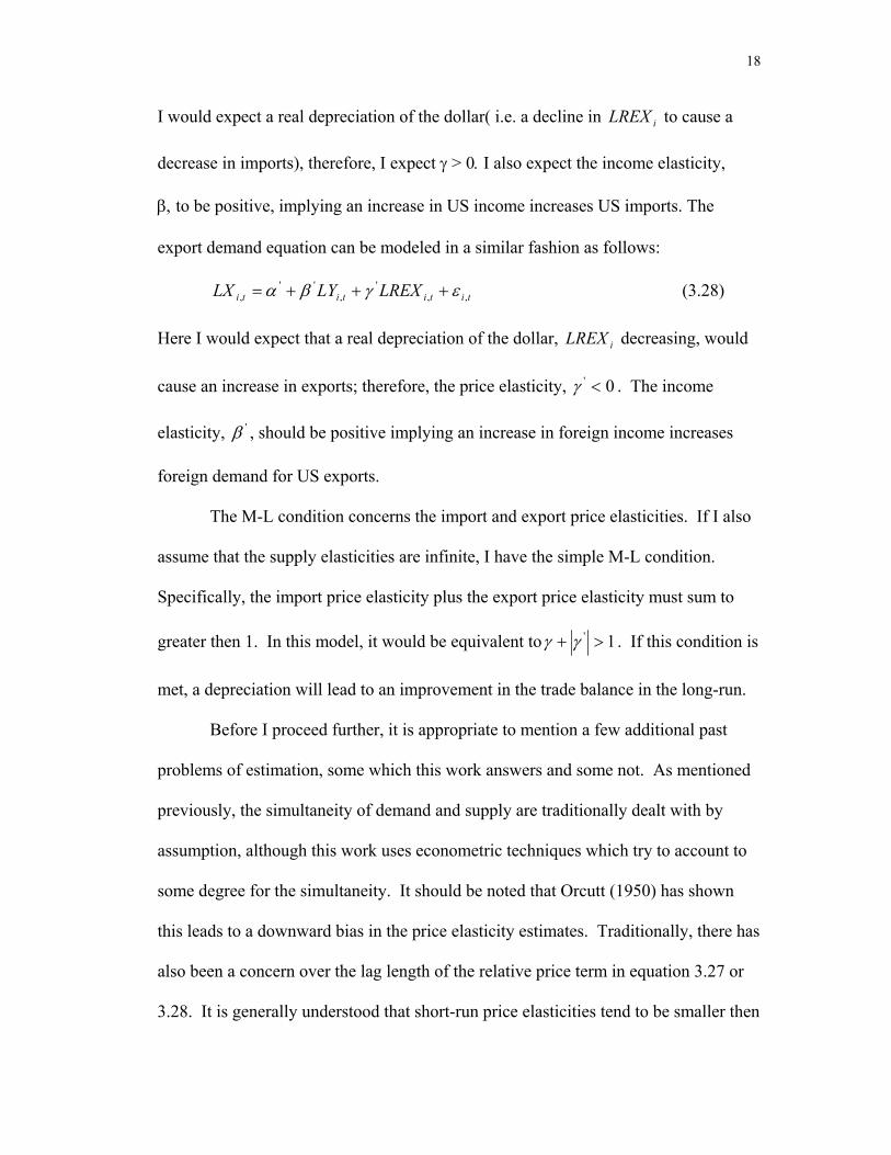
I would expect a real depreciation of the dollar( i.e. a decline in iLREX to cause a
decrease in imports), therefore, I expect γ > 0. I also expect the income elasticity,
β, to be positive, implying an increase in US income increases US imports. The
export demand equation can be modeled in a similar fashion as follows:
titititi LREXLYLX ,,'
,''
, εγβα +++= (3.28)
Here I would expect that a real depreciation of the dollar, iLREX decreasing, would
cause an increase in exports; therefore, the price elasticity, 0' <γ . The income
elasticity, 'β , should be positive implying an increase in foreign income increases
foreign demand for US exports.
The M-L condition concerns the import and export price elasticities. If I also
assume that the supply elasticities are infinite, I have the simple M-L condition.
Specifically, the import price elasticity plus the export price elasticity must sum to
greater then 1. In this model, it would be equivalent to 1' >+ γγ . If this condition is
met, a depreciation will lead to an improvement in the trade balance in the long-run.
Before I proceed further, it is appropriate to mention a few additional past
problems of estimation, some which this work answers and some not. As mentioned
previously, the simultaneity of demand and supply are traditionally dealt with by
assumption, although this work uses econometric techniques which try to account to
some degree for the simultaneity. It should be noted that Orcutt (1950) has shown
this leads to a downward bias in the price elasticity estimates. Traditionally, there has
also been a concern over the lag length of the relative price term in equation 3.27 or
3.28. It is generally understood that short-run price elasticities tend to be smaller then
19
long-run price elasticities, due to the fact that trade relationships are sticky and less
price responsive in the short-run. The econometric technique that I employ in this
work is particularly well suited for estimating the long-run elasticities, and doesn't
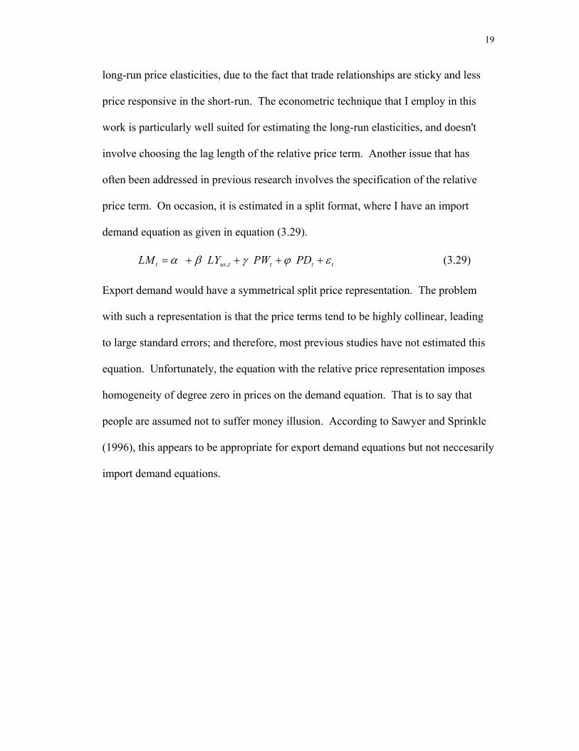
involve choosing the lag length of the relative price term. Another issue that has
often been addressed in previous research involves the specification of the relative
price term. On occasion, it is estimated in a split format, where I have an import
demand equation as given in equation (3.29).
ttttust PDPWLYLM εϕγβα ++++= , (3.29)
Export demand would have a symmetrical split price representation. The problem
with such a representation is that the price terms tend to be highly collinear, leading
to large standard errors; and therefore, most previous studies have not estimated this
equation. Unfortunately, the equation with the relative price representation imposes
homogeneity of degree zero in prices on the demand equation. That is to say that
people are assumed not to suffer money illusion. According to Sawyer and Sprinkle
(1996), this appears to be appropriate for export demand equations but not neccesarily
import demand equations.

20
Chapter IV
Aggregation Issues
One of the fundamental arguments of this work is that the level of aggregation
employed in most previous research is subject to bias and useless for policy makers.
The aggregation bias critique is not new to import and export demand elasticity
estimation; see for example Magee (1975), Orcutt (1950), Leamer and Stern (1970),
and Goldstein and Khan (1985). Magee (1975) illustrates the potential bias by
demonstrating that the average product price change times the average elasticity will
generally not give the correct quantity change instigated by a policy-induced price
change. The reason is that if product price changes are negatively related to their
elasticities, then the actual quantity change will be less than the product of the total
elasticity times the aggregate price change. Effectively, items with large prices are
given too much weight in the aggregate elasticity. For a detailed example of this, see
appendix 3. Here I will demonstrate the potential bias in a simple example from
Magee (1975).
A paper by Pesaran and Barker (1990) they suggests that the applied
researcher should ask four questions when deciding on the appropriate level of
aggregation for their work. They are as follows: (1) What is the purpose of the
exercise? (2) What are the specification errors involved? (3) What data are
available? (4) What is the attitude of the investigator towards the postulates of
simplicity and parsimony? I will address each of these questions in turn.
What is the purpose of the exercise? As Pesaran and Barker (1990), herein
PB, suggest, this question is crucial in the design of the research. They suggest that a

21
desire to prescribe policy ought to pursue a high level of detail only attainable
through disaggregation. If, however, the researcher is only interested in describing a
phenomenon, where only the sign of a coefficient matters and not its size then they
need not disaggregate. In fact in the latter case PB suggest aggregating to provide
general conclusions. Since this work is concerned with policy prescription however, I
will disaggregate along country lines.
Question 2 asks, What are the errors of specification? Pesaran and Barker
(1990) make the fundamental point that it is better to estimate a correctly specified
model than an incorrectly specified model. This obvious suggestion could involve
estimating disaggregated demand equations even if the research question is only
concerned with forecasting the aggregate demand for imports and exports.
Question 3 asks pragmatically about the availability of data. Generally, data
are not available on a highly disaggregated basis and, therefore, the researcher is
often constrained. Here I are constrained by several factors. While trade is available
on a highly disaggregated basis, it is generally disaggregated by commodity or
country only; but, not both. Since I are interested in the total bilateral trade balance
and not the total trade balance for a particular commodity I should disaggregate on a
country basis.
Next I will address question 4 which concerns the degree of simplicity of the
model. PB argue that a simple model should be preferred to a more complex model
ceterus paribus, often this criticism is more superficial than substantive. Peseran and
Baker (1990) argue that, all else equal, a more simplistic and parsimonious model
should be preferred to a model which is less so.

22
Finally, PB point out that when a researcher has a disaggregated model
correctly specified, free from measurement and the appropriate data, they can do no
worse and, in fact, may do better than an aggregate model. I believe that the bilateral
trade model employed in this work satisfies these criteria. That is to say, it is no more
suscpetible to measurement error, or mispecification than its aggregate counterpart.
The aggregation bias holds not only for aggregation over commodities, but
also for aggregation over time. The next section discusses the types of aggregation
and their relevance to the current work.
4.1 Cross Sectional
The problem with choosing the level of aggregation is that there are very few
distinct points. Aggregation can be thought of as a continuum. At the disaggregated
end I have data for individual products (i.e. specific brands), their prices, and the
quantities of each imported and/or exported. On the aggregate side of the continuum,
I have data for total imports and exports to and from the rest of the world. Clearly,
there are many compromises along the way, but there are at least two distinct points
of disaggregation. The first involves disaggregating trade on the basis of
commodities classes and the second involves disaggregating trade on the basis of
country origin or destination. As an example one could disaggregate commodities
based on their Standard Industry Classification Codes and then estimate the
elasticities for particular commodity classes. I will discuss this further in section
4.1.1 and in section 4.1.2 I will discuss the case where the disaggregation is based on
the commodity's country of origin or destination.
4.1.1 Commodity

23
As I previously mentioned I can disaggregate merchandise trade by
commodity. This is not done for several reasons. First, it isn’t the best answer to
Peseran and Barker’s question 1. That is to say it fails to address the policy question
of whether a coordinated depreciation will improve a countries bilateral trade balance.
Second, I would need data on all commodities exported to the G-7 countries from the
US and imported by the US from the G-7 countries. This data if and when available
is subject to enormous measurement error due to the desire to cheat on tariffs.
4.1.2 Country
Alternatively I suggest disaggregating on a bilateral basis, which according to
Goldstein and Khan (1985) can be viewed as a form of cross-sectional commodity
aggregation since certain countries tend to export and import certain classes of goods.
This level of aggregation will best answer the four questions of Pesaran and Barker
(1990). It speaks directly to the purpose of the exercise, to test whether a bilateral
depreciation can improve the trade balance. It also minimizes the potential
specification errors, since there is no need to proxy world income as is the case in the
aggregate export demand equation. Additionally the data are available and relatively
easy to attain and are subject to less measurement error than the individual
commodity data.
4.2 Temporal
Deciding on the level of temporal aggregation, is nothing more than deciding
on the frequency of the data to use. As is noted in the econometric section below,
little is to be gained, in the way of increased power, through larger sample size by
increasing the frequency of the data. In fact Pierse and Snell (1995) and Shiller and

24
Perron (1985) show that time span is important and not the number of observations.
In addition I can not get accurate GDP data on a monthly basis. It is then prudent to
use quarterly data, as do most other works.

25
Chapter V
Econometric Techniques
5.1 Unit Roots
The identification of non-stationarity as a problem in econometric analysis is a
fairly recent event. The problem, described initially in the seminal piece of Granger
and Newbold (1974), highlights the extreme shortcomings of Ordinary Least Squares
when the regression involves non-stationary variables. They independently generated
two random walks shown in equation (5.1) and (5.2)
t t ty y= +
−1 ε (5.1)
t t tz z= +−1 ε (5.2)
They then regressed one on the other using OLS, given in equation (5.3), and
incorrectly found a statistically significant relationship 75% of the time.
t t ty z= + +α β ε (5.3)
The assumptions of the classical model require ty and tz to be stationary and
have errors whose mean is zero and variance is finite. Granger and Newbold (1974)
show that an ordinary least squares regression can be spurious in the face of non-
stationary variables, the r-squared may be high, and t-statistics significant, even
though there is no relationship. The output looks good because OLS does not give
consistent estimates and the asymptotics of the t-test are non-normal. Later, Phillips
(1986) gave this problem a more theoretical treatment. However, it was Nelson and
Plosser (1982) that demonstrated the existence of unit roots and non-stationarity in
most macroeconomic time series.

26
At this point it would help to elaborate on the theoretical existence of a unit
root. Let us propose the following general model:
( ) ( ) tt LByLA ε= (5.4)
where ( )LA and ( )LB are polynomials in the lag operator. If all the roots of
( ) 0=LA lie outside the unit circle, then ty is a stationary ARMA process; but, if at
least one root lies on the unit circle, then the process is non-stationary, and contains a
unit root. The series is also referred to as being integrated of order one, I(1).
The problem with many empirical works on trade elasticities is that they very
seldom address the issue of non-stationarity. It is visually obvious from a graph of
the data that most all variables under consideration are non-stationary. Figures 5
through 29 clearly demonstrate non-stationarity, since the data do not revert to a
mean in a timely fashion. Less clear visually is whether the series can be
characterized by a stochastic trend (unit root) or a determinist trend. In order to make
this determination, I must apply a more rigorous empirical test. Very few of the
numerous articles that estimate the price elasticities actually test the data in order to
distinguish between these types of non-stationarity.
In this work, I will apply a two different unit root tests. The first test used
extensively in other works is the Augmented Dickey-Fuller test, herein ADF. The
null hypothesis of the ADF test is that a unit root can characterize the series, and the
series is in fact non-stationary. Unfortunately, this test suffers from very low power,
particularly in small samples; so, I will also implement a test attributed to
Kwiatkowski et. al. (1992), herein KPSS. This second unit root test adopts as the null
hypothesis the characterization of the series as a mean stationary process, or a trend

27
stationary process. It, therefore, transposes the null and alternative hypotheses of the
ADF test.
The ADF test has been explored at length in the literature. For a thorough
explanation of the procedure see Bahmani-Oskooee (1991) and Chueng and Chinn
(1994). Here I will simply discuss the estimation methods. The ADF tests involves
estimating via OLS, equation (6.15).
t
p
iittt uyyty +∆+++=∆ ∑
=−−
110 γδα (5.5)
The test concerns the coefficient of the lagged dependent variable, γ . The null
hypothesis is, 0:0 =γH . Due to the potential non-stationarity of the error, the
traditional t distribution is non-normal and involves nuisance parameter
dependencies. The results of the ADF test can be found in Table 1, where the choice
of augmenting lag was made using the Akaike Information Criterion, herein AIC, and
the Schwartz Bayesian Criterion, herein SBC. It appears in parenthesis following the
test statistic. In all cases for all variables, I fail to reject the null hypothesis that the
series contains a unit root. The first two columns include only an intercept in the
estimating equation, while the last two columns include an intercept and a trend. The
results suggest overwhelmingly that the data are in fact non-stationary; but, it would
be prudent to further consider this question, since the ADF test is known to suffer
from low power. Toward this end, I will apply the KPSS test.
The KPSS test is a more recent innovation in the literature and, as such, has
been applied less frequently; however for good discussions of the procedure see
Cheung and Chinn (1994) and Bahmani-Oskooee (1998b). It is worth mentioning a
few things about the test before I proceed. The KPSS test amounts to a Lagrange

28
Multiplier test with the Null hypothesis of trend stationarity or level stationarity. It
decomposes the process to a random walk and stationary error, for the test of level
stationarity, and a deterministic trend is included in the case where the null hypothesis
is trend stationary. Equations (5.6) and (5.7) show this decomposition, where t is a
constant or a linear trend depending upon the test.
t t tZ a t r= + + ε (5.6)
t t tr r u= +−1 (5.7)
The KPSS test then amounts to a test of the variance of the random walk component,
equation (5.7), with the null hypothesis equivalent to a residual with zero variance.
The test statistic is constructed as follows:
− ∑2 2 2T S st l/ ( ) (5.8)
where
t ii
t
S e==∑
1
(5.9)
and ie are the residual from equation (5.6)
2 1 2
1
1
1 12s T e T e el w s lt
t
T
s
l
t t st s
T
( ) ( , )= +−
=
−
=−
= +∑ ∑ ∑ (5.10)
the Bartlett window was chosen so
w s l s l( , ) /= − +1 1 (5.11)
The test requires choosing the lag truncation of spectral window. I use the Bartlett
window as suggested in KPSS (1992), but I take a rather agnostic approach to the
choice of the lag truncation parameter due to the size and power distortions in finite
samples and under different specifications of the error.

29
The null hypothesis of the KPSS test is mean stationary if a trend is excluded
from equation (5.6), and trend stationary if it is included. The null hypothesis test for
u2 0σ = . The alternative hypothesis suggests the series is better described as a unit
root process (non-stationary). In Table 2, I report the test statistic for the null of mean
stationarity for lags 1-8; and in Table 3, I report the results of the KPSS test with
trend stationarity as the null hypothesis. The evidence here is not as overwhelming as
the ADF, but still convincing. For a lag truncation parameter of 0 and a 10%
significance level, I can reject the null for all series in both the trend and mean
stationarity case.
The results of the ADF and KPSS tests can be used together as suggested by
Cheung and Chinn (1994, forthcoming), to develop a 2 by 2 matrix. The first cell, the
upper left hand corner, consists of failing to reject the null hypothesis for both the
ADF and KPSS tests. Chueng and Chinn argue that this demonstrates the lack of
power the tests have in small samples. They argue the series are not informative
enough to classify the variable as I(1) or I(0), so the prudent measure is to proceed
under the assumption that the series are I(1). The second cell represents failing to
reject the null of the ADF test and rejecting the null of the KPSS test. This
corresponds to a robust acceptance of the existence of a unit root. Since all of the
series fit into this category I proceed under the assumption that they contain a unit
root. The third cell, where I reject the ADF null and fail to reject the KPSS null, is a
robust acceptance of stationarity. The fourth and final cell represents the rejection of
both nulls. This is possibly a nonsensical result or an indication of a fractional or
explosive root.

30
Fail to Reject KPSS Null Reject KPSS Null
Fail to Reject ADF Null Low Power of tests I(?) I(1)
Reject ADF Null I(0) Nonsensical results I(?)
5.2 Cointegration
Now that I have determined the order of integration, I can proceed with our
cointegration tests. Since I are interested in the long-run relationship between the
variables and in particular the estimates of the long-run elasticities, testing for the
existence of cointegration among the variables is an appropriate method to employ.
Cointegration roughly captures the long-run stationary relationship between two or
more non-stationary variables. For this task, I have chosen Johansen-Juselius’ Full
Information Maximum Likelihood (FIML) estimation technique (1990).
5.2.1 OLS
In order to appreciate the improvement in coefficient estimates from using the
proper econometric technique, it will be of some use to apply the previously used
methods to these data. I will trace the progress of the econometric literature through
the estimation of the import and export demand equations, (3.27) and (3.28)
respectively. Initially I estimate these equations using OLS for each country. The
results can be found in Table 4. The last column in the table gives the Durbin-
Watson test statistic for serial correlation. It is clear that in all cases the residuals
display a high degree of serial correlation, with the Durbin-Watson below the lower
critical bound of 1.623. It is also important to note that the estimates of the M-L
condition, found in Table 5, suggest that, in fact, depreciation will not improve the
bilateral US trade balance. One should be careful with the output from an OLS

31
regression with non-stationary variables. This is demonstrated in section 5.1, in
which I noted the invalidity of t-statistics in this case. Furthermore, this estimation is
potentially a spurious one, if the residuals are also non-stationary. If, however, the
residuals from this regression are stationary, then the variables are referred to as
cointegrated. Generally speaking, cointegration refers to a linear relationship
between I(d) variables whose residuals are I(d-b), where b=> 1.
Most studies after Stern et al. (1975) recognized the problem of serial
correlation and attempted to correct for it. I too use the Cochrane-Orcutt method to
correct the elasticity estimates for first order serial correlation, and they are found in
Table 6. The estimates of the price elasticities are generally smaller then the
estimates with no correction. In fact, Table 7 gives the estimates of the M-L
Condition when correcting for serial correlation, and every country has a lower
estimate. Again, the conclusion would be that the US does not satisfy the M-L
condition on a bilateral basis with the rest of the G-7.
While I have applied OLS to the demand equations knowing that the variables
are non-stationary, I may not have been far from the proper technique. Engle-
Granger (1987) show that if there are two variables that are I(1), but a linear
combinations of the two are I(0), then they are cointegrated. That is to say, they have
a stable long-run relationship. They further suggest that the relationship be estimated
using OLS which provides “hyper” consistent parameter, although the t statistics are
still invalid. They then test the residuals for stationarity using the ADF test with
adjusted t-statistics. It should be noted that Table 7 provides estimates of RHO, the
first order autoregressive coefficient, which in all cases is less then one.

32
ttt uu ερ += −1 (5.12)
This implies stationary residuals and, therefore, a cointegrating relationship. The
problems with this procedure, which was used by Rose(1991) and Rose and
Yellen(1989), are many. First is the problem of including endogenously determined
regressors. Another problem occurs because it provides estimates on only one
cointegrating relationship when, in fact, there may be as many as 2 in my case.
Finally, the Engle-Granger method estimates the short-run and long-run responses in
separate stages. The next section uses a technique proposed by Phillips and Hansen
(1990) to overcome the problem of endogeneity.
5.2.2 Fully Modified OLS
The first cointegration method I use is based on Phillips and Hansen (1990),
referred to as Fully-Modified Ordinary Least Squares (FM-OLS). This method
proposes a semi-parametric correction for serial correlation of the residuals and the
endogeneity of the regressors. It, like the KPSS test, involves a choice of spectral
window and lag length. In this work I use, the Bartlett window and a lag length of 8.
I now turn to the application of FM-OLS to equations (3.27) and (3.28), the
results of which are given in Table 8. It is clear that the semi-parametric correction
results in larger price elasticity estimates. This supports the monte carlo simulations
in Phillips and Hanson (1990) where they show that the FM-OLS has a much smaller
bias then OLS in small samples. In fact, for every country the estimate of the M-L
condition by FM-OLS is larger then the estimate for OLS or OLS with a correction
for serial correlated errors (see Tables 9,7, and 5). Further inspection reveals that the
source of the increase stems from an upward revision in the estimates of all export

33
demand price elasticities, whereas, the import demand price elasticity for Canada,
Germany, and Italy are revised downward. While the sum of the export and import
demand price elasticities are larger then the previous estimates, they still sum to less
then unity. The FM-OLS estimates the US does not satisfy the M-L condition on a
bilateral basis. In fact, Italy and the U.K. are the closest to satisfying the M-L
condition with estimates of 0.978 and 0.908 respectively.
Another interesting result from the application of FM-OLS involves the
apparent lack of change in the income elasticities. In fact, none changes by more then
10%. The asymmetry in elasticities noted earlier, where income elasticity of US
exports is much lower then the US import income elasticity, is thus retained. It
appears that, while previous authors underestimate the price elasticities, they correctly
estimated the income elasticity.
5.2.3 Error-Correction Modeling
Johansen-Juselius’ Full Information Maximum Likelihood (FIML) estimation
technique (1990) is a multivariate cointegration technique, where the cointegrating
relationship is estimated within a dynamic vector autoregressive. This method should
be preferred to the Engle and Granger (1987) and the Phillips and Hansen (1990)
methods. Unlike the previous two methods Johansen's for more then one
cointegrating vector and also estimates the entire model simultaneously, while
allowing for the endogenous determination of the regressors.
One shortcoming of Johansen's method is that the results are sensitive to the
lag length chosen for the vector autoregression (VAR) (see for example Toda, 1994;
and Bahmani-Oskooee, 1995). I use Akaike’s information criterion (AIC) and the

34
Schwarz Bayesian Information Criterion (SBC) from the unrestricted VAR in levels
to select the lag length. This method is suggested by Sims (1980) and involves
estimating equation (5.13).
t t q t q tX A A X A X= + + + +− −0 1 1 . .. ε (5.13)
The AIC is then constructed as
[ ]12
2( ) log ( ) ( )T q DET S q k q k− + + (5.14)
and the SBC is constructed as
[ ] )log()()(log)( 221 qTkqkqSDETqT −++− (5.15)
where ( )[ ]qSDET is the determinate of the variance-covariance matrix of the
unrestricted VAR(q) in levels. Generally, the lag length associated with the smallest
AIC or smallest SBC is chosen; however, it should be noted that the statistics
presented in Table 10 are based upon the maximum likelihood version of equations
(5.14) and %.15). Therefore, the proper lag is the one with the largest AIC or SBC.
When comparing these criteria across lag lengths it is important to correct for sample
size differences. All statistics in Table 10 are, therefore, based upon the same sample
from 1975Q1 to 1996Q2, which corresponds to a maximum lag length of 8.
Traditionally in other studies such as Carone (1996), the lag length is chosen
arbitrarily. If the data are quarterly, then they choose 4 lags, if the data are monthly,
12 lags. The results of my work suggest that this may be a good approximation for
the export demand equations, but it leads to an overparameterization of the import
demand equations. This is true when compared to the AIC; however, when using the
SBC to select lag length, the models are always more parsimonious then when using
4 lags. Kiviet and Phillips (1992) show that there is only one optimal lag length for a

35
particular data generating process (DGP). They further show that insufficient lag
length leads to an underparameterization of the model and an over rejection of the
null of no cointegration. Conversely, a lag length that is too long results in the over
parameterization of the model; and thus, the cointegration tests display a loss in
power.
Once the proper order of the VAR has been selected, the next step is to test for
cointegration. The Vector Error Correction Model (VECM) of order q can be
summarized as follows:
t
q
iititt XXAX ε+∆Π+Π+=∆ ∑
=−−
1100 (5.16)
where tX consists of a vector of all I(1) variables, shown in (5.17) and (5.18), where
the variables come from equation (3.27) and (3.28)
=
t
t
t
t
LREXLYUSLM
X (5.17)
=
t
t
t
t
LREXLYUS
LXX (5.18)
The test for cointegration in the Johansen-Juseluis method tests for the
reduced rank of the coefficient matrix of the lagged variables in levels, 0Π in
equation (5.16). The rank of the matrix represents the number of cointegrating
vectors that exist. That is to say, it represents the number of unique stationary linear
combinations of the non-stationary variables. I use Johansen's lambda-trace and

36
lambda-max tests for reduced rank. These amount to significance tests of the
eigenvalues of 0Π . If the rank of 0Π is greater then zero and less then full, then the
variables are cointegrated with the number of cointegrating vectors equal to the rank.
If the rank is equal to zero, then there are no cointegrating relations between the
variables, and the VECM is a stationary VAR in differences. However, if 0Π is of
full rank, then the variables are stationary. That is to say the variables of the VAR
have non stochastic trends, a direct contradiction to the unit root tests. Equation
(5.19) gives the trace statistic and equation (5.20) gives the max statistic
trace i
i r
n
r Tλ λ( ) ln( )= − −= +∑ 1
1
(5.19)
max ( , ) ln( )λ λr r T r+ = − − +1 1 1) (5.20)
The results of max and trace tests can be found in Tables 11,and 12 for the
case where the lag was chosen by the AIC. Tables 15 and 16 provide the results of
the max and trace tests for the case where the lag was chosen with the SBC. The
results using the AIC lag selection criterion suggest there is at least one cointegrating
relationship for import and export demand for all countries except Canada. The US
import demand from Canada fails to support the existence of a cointegrating
relationship according to the trace or max tests at the 10% significance level. Using
the SBC lag selection criterion, there is evidence of at least one cointegrating relation
for all countries. For most countries there are often two cointegrating vectors for
import and export demand. This result is expected and follows from Kiviet and
Phillips (1992). Since the SBC always selects a more parsimonious model then the
AIC, the results are a possible over rejection of the null of no cointegration.

37
Once I have determined the number of cointegrating vectors, I can turn to the
estimates of those cointegrating vector(s). The estimates of the long-run relationship
can be extracted from the coefficient matrix, βα ′=Π0 , where β represents the
cointegrating vector(s). The researcher is faced with the decision of which variable to
normalize in the β vector. Given that the current research is interested in the
relationships in equations (3,27) and (3.28), it is appropriate to normalize on the log
of imports in the case of import demand, and the log of exports in the case of export
demand. Having done that, the estimates are presented in Table 13, which uses the
AIC lag selection method; and Table 17, which uses the SBC lag selection method.
First turning to the AIC estimates of Table 13. In the case of one
cointegrating vector, the choice of price elasticities is unambiguous, however, for
French and Italian imports as well as Italian and Japanese export demand, I am faced
with two price elasticity estimates. King et al. (1991) suggest using the estimates of
the cointegrating vector which most closely matches the relevant economic theory.
For our purpose, the appropriate cointegrating vector is the one that displays the
appropriate sign and size. A real depreciation should discourage imports. Therefore,
the import demand price elasticity should be positive, since a depreciation is defined
as a decrease in the real exchange rate.
After selecting the appropriate cointegrating vector, it is evident the
elasticities tend to be larger then the OLS and FM-OLS estimates. This can be seen
in the estimates of the M-L condition presented in Table 14. France, Italy, Japan, and
the U.K. elasticities sum to greater then unity, while Germany's sum to slightly less.
It should be noted that, while Canada is included in these tables, it is simply for

38
completeness. Since there is no cointegration for the import equation, it is
inappropriate to comment on the elasticity estimates derived from it. Unlike the OLS
estimates, there is now cause for optimism. It appears that a depreciation will in fact
improve the bilateral trade balance between the US and France, Italy, Japan, and the
U.K.
Now I will turn to the estimates of the cointergating vectors when the SBC is
used to select the lag length. In this case I find that there is at least one cointegrating
vector for all countries. In fact only the US import demand from Canada and
Germany and US export demand from Canada and Italy contain only 1 cointegrating
vector. The estimates of all cointegrating vectors are presented in Table 17. Again,
following King et al. (1991) I report the M-L condition estimates using the
theoretically appropriate elasticities and they can be found in Table 18. Here I have
Germany, Japan, and the U.K. demonstrating large enough elasticities to satisfy the
M-L condition, while France and Italy fall just short at 0.90 and 0.70 respectively.
There is reason to believe that the demand equations for Canada are misspecified,
because the export demand elasticity estimates very large at -58.25. Additionally the
import demand price elasticity carries the wrong sign at -0.65.
This work seems to suggest that there is good reason to believe that the U.S.
satisfies the M-L condition on a bilateral basis with all of the remaining G-7 countries
except Canada. Leaving aside Canada for the moment and looking to the remaining
countries. Japan and the U.K. satisfy the M-L condition using both the AIC and the
SBC, while Germany satisfies it using the SBC and Italy and France satisfy it using
the AIC. Even though these results are less robust for the latter three countries it is

39
clear that depreciation would improve the bilateral trade balance given I are currently
carrying a large deficit with that country. As is shown in appendix A, the M-L
condition is overly stringent in this case.
Returning to the case of Canada, it appears as though the model is
misspecified in some way. One possible explanation involves the recent trade
agreement between the U.S., Canada, and Mexico. The agreement known as the
North American Free Trade Agreement, herein NAFTA, was implemented in 1994.
This introduces a potential structural change in the import and export demand
relationships that are not entirely captured by the real exchange rate. Still another
explanation highlights important factors that are not included in the model such as the
resistance to terminating trade relationships, and therefore a decreased price
sensitivity.
5.3 Stability Tests
Once the income and price elasticities are estimated I might naturally inquire
about their stablity. If in fact the cointegrating vectors and therefore the price
elasticities are unstable over time policy prescription based on the estimated
elasticities would be unwarranted, or at least risky. There are many possible methods
for testing the stability of the cointegrating vector(s). I will apply at least two tests
for the stability of the error-correction model, the cumulative sum of recursive
residuals (CUSUM) and cumulative sum of the square of the recursive residuals
(CUSUMSQ), due to Brown et al. (1975). These tests are visual and require plotting
the test statistic, which is a function of time, and the appropriate confidence interval.
If the test statistic meanders outside the confidence interval it suggests a possible
40
structural break or non-constancy of the parameters. More formally, the test involves
several stages. I first estimate the vector error correction equation given in equation
(5.16), using the lag selected by the AIC. Then I fix the cointegrating vector(s) and
decompose the vector error correction equation by each variable as follows.
∆∆∆
=∆
t
t
t
t
LREXLYUSLM
X (5.21)
This represents the import demand system of equations and similarly for the export
demand system I can decompose the vector into the variables of interest.
∆∆
∆=∆
t
t
t
t
LREXLYUS
LXX (5.22)
I can then concentrate on the first equation in each model, the import demand
equation or the export demand equation, and estimate it consistently with OLS. From
here forward I will focus on the import demand equation, but the same arguments
apply to the export demand equation. I use the data up to and including t-1 to
estimate the coefficients of the single equation Autoregressive Distributed Lag
Model, given in equation (5.23).
++=∆ −− 2101 tt ECLM ββ
( ) 11
111 −=
−−−−−− +∆+∆+∆∑ t
p
iitiitiiti LREXLYUSLM εθφγ (5.23)
I then calculate the one step ahead prediction error defined in equation (5.24)
∧∆−∆= ttt LMLMv (5.24)
41
Where ∧
∆ tLM is the one step ahead prediction using the coefficients estimated in
equation (5.23), and the data up to point t. I can similarly calculate the export
demand one step ahead prediction error. Then define the scaled recursive residuals as
).(. t
tt ves
vw = (5.25)
The CUSUM test statistic is then
∑+=
=t
kjjt wW
1
t=k+1, …, n (5.26)
The CUSUMSQ test statistic is
∑
∑
+=
+== n
kjj
t
kjj
t
w
wS
1
2
1
2
t=k+1, …, n (5.27)
If the estimated parameters are constant then the one step ahead prediction errors
should be white noise such that their sum is always zero. The CUSUM and
CUSUMSQ statistics are plotted against the 5% critical lines, for import and export
demand for each country. They appear in Figures 30-53.
The CUSUM test results suggest that for all countries the bilateral import and
export demand relationships have been stable. Hanson (1991) suggests that this test
be view as an intercept constancy test. Therefore it appears as though the intercept
has remained constant for import and export demand equations for all countries.
Hanson (19991) also suggests that the CUSUMSQ test is equivalent to a test of the
stability of the variance of equation (5.23). The variance appears to be stable for all
countries except U.S. import demand from France, Italy and the U.K., while the

42
Japanese export demand appears to be unstable. It should again be noted that the
CUSUM and CUSUMSQ results are reported for Canadian export demand simply for
completeness since there was no evidence of cointegration using the AIC lag
selection.

43
Chapter VI
Summary and conclusion
The emphasis of this work is to provide more reliable estimates of income and
price elasticities of import and export demand to policy makers so that they may
make more informed public policy decisions. Specifically I estimate these elasticities
on a bilateral basis between the US and each of the following countries: Canada,
France, Germany, Italy, Japan, and the UK. These elasticities can be used to test the
M-L condition, if it is satisfied the estimates can then the US can improve its bilateral
trade balance by depreciating its currency vis-à-vis the partner country. The
elasticities are then used to calculate the size of the depreciation needed to improve
the trade balance. Previous work has generally done this on an aggregate basis,
however in an attempt to improve the estimates I argue that it is critical to choose the
appropriate level of aggregation for the estimation of these elasticities. The factors
important in determining this level include the policy makers potential policy tools,
data availability, and econometric concerns. Therefore it is clear that the bilateral
approach in this paper is superior given the objectives.
I also further improve the estimates of the trade elasticities by employing
recent econometric innovations. Johansen’s method is applied to the estimation of
the import and export demand equations, along with several other cointegration
techniques. The results indicate that the US satisfies the M-L condition on a bilateral
basis with all of the countries except Canada. Therefore a devaluation of the dollar
vis-à-vis the other 5 currencies should improve the US bilateral trade balance with
those countries.

44
There are several other important conclusions in this work. It confirms, on a
bilateral basis, the disparity in income elasticities noted in the aggregate case by
Sawyer and Sprinkle (1996), and others. That is the US import demand income
elasticity is larger then the export demand income elasticity. In fact this is probably a
plausable explanation for the failure of the trade balance to improve after the dollar
started to fall in 1985.
While this study has advanced the literature on several fronts there are some
shortcomings that will be addressed in future work. Elasticities could be estimated
for major commodity classes, which would provide a better description of the impact
of a depreciation on each sector of the economy. Additionally it would remove
another layer of aggregation, and further reduce any potential bias associated with it.
The other major shortcoming of this work is that it does not address the means by
which a policy maker induces and sustains a real depreciation, nor does it address all
the potential consequences of such an action. A further examination of these issues
may relegate this work to the level of a simple intellectual exercise, unable to be
applied in practice. It could therefore be the most perverse of all arguments made
Ceterus paribus.

45
TABLES
Table 1: The ADF Unit Root Test Statistics. Intercept only Intercept and Trend Variable AIC SBC AIC SBC US LY -1.54(1) -1.54(1) -2.96(1) -2.96(1) Canada LY -1.84(1) -1.84(1) -2.32(1) -2.32(1) LREX -1.34(4) -1.73(3) -2.77(3) -2.77(3) LM -0.03(5) -0.41(4) -2.28(4) -2.28(4) LX 0.37(8) -0.21(4) -1.42(8) -2.06(4) Japan LY -3.06(1) -3.06(1) -0.19(1) -0.19(1) LREX -1.55(1) -1.55(1) -2.33(1) -2.33(1) LM -1.71(1) -1.71(1) -1.41(1) -1.41(1) LX 0.05(2) -0.19(1) -3.14(1) -3.14(1) Germany LY -0.17(1) -0.17(1) -1.44(1) -1.44(1) LREX -1.76(1) -1.76(1) -1.94(1) -1.94(1) LM -1.25(4) -0.69(1) -3.24(8) -1.80(1) LX -0.62(4) -0.62(4) -1.93(4) -1.93(4) UK LY -0.44(8) -0.64(3) -2.39(8) -1.53(1) LREX -2.10(1) -2.10(1) -2.22(1) -2.22(1) LM -0.91(1) -0.91(1) -1.97(1) -1.97(1) LX -0.47(4) -0.31(2) -2.65(5) -1.93(2) France LY -1.63(2) -1.62(1) -3.08(2) -3.08(2) LREX -1.95(1) -1.95(1) -2.08(1) -2.08(1) LM -0.91(1) -0.91(1) -1.97(1) -1.97(1) LX -1.61(8) -1.26(4) -3.04(8) -3.04(8) Italy LY -2.59(3) -2.61(1) -2.64(1) -2.64(1) LREX -1.65(1) -1.65(1) -2.30(1) -2.30(1) LM -1.00(2) -1.00(2) -2.40(2) -2.40(2) LX -1.66(8) -1.66(8) -2.90(8) -2.90(8) 95% Critical Value -2.90 -2.90 -3.46 -3.46 _____________________________________________________________________ Note : The critical values come from MacKinnon (1991 Table1) and the augmenting lag was selected by the AIC or SBC and appears in parenthesis behind the statistic

46
Table 2: The KPSS Test for Mean Stationarity for All Variables. (The 5% critical value is 0.463, 10% is .347) Lag Truncation Parameter Variable 0 1 2 3 4 5 6 7 8 US LY 3.095 2.332 1.876 1.573 1.357 1.195 1.070 0.969 0.886 Canada LY 3.053 2.303 1.855 1.557 1.345 1.186 1.063 0.965 0.885 LREX 1.733 1.309 1.058 0.892 0.776 0.690 0.625 0.570 0.522 LM 2.730 2.074 1.675 1.410 1.219 1.077 0.968 0.876 0.799 LX 2.724 2.075 1.677 1.413 1.222 1.079 0.969 0.877 0.800 Japan LY 3.144 2.367 1.902 1.593 1.372 1.207 1.079 0.977 0.893 LREX 1.919 1.451 1.175 0.993 0.864 0.770 0.698 0.635 0.580 LM 2.929 2.205 1.771 1.483 1.277 1.124 1.006 0.910 0.832 LX 2.845 2.150 1.733 1.456 1.259 1.110 0.995 0.899 0.818 Germany LY 2.963 2.233 1.796 1.506 1.299 1.145 1.025 0.927 0.846 LREX 0.484 0.367 0.298 0.253 0.221 0.198 0.181 0.165 0.150 LM 2.532 1.916 1.542 1.295 1.118 0.987 0.886 0.801 0.730 LX 2.283 1.750 1.430 1.213 1.052 0.932 0.838 0.760 0.694 UK LY 3.055 2.300 1.848 1.547 1.334 1.174 1.050 0.949 0.866 LREX 0.708 0.539 0.440 0.376 0.331 0.298 0.274 0.251 0.230 LM 2.801 2.135 1.728 1.453 1.256 1.107 0.992 0.898 0.820 LX 2.561 1.955 1.591 1.344 1.165 1.031 0.927 0.842 0.770 France LY 3.037 2.291 1.846 1.540 1.339 1.181 1.059 0.960 0.880 LREX 0.424 0.322 0.262 0.223 0.196 0.177 0.162 0.147 0.135 LM 2.948 2.231 1.796 1.506 1.298 1.143 1.023 0.926 0.845 LX 2.434 1.848 1.500 1.265 1.094 0.966 0.868 0.786 0.717 Italy LY 3.062 2.311 1.862 1.563 1.350 1.190 1.066 0.967 0.885 LREX 1.371 1.037 0.841 0.711 0.620 0.553 0.502 0.456 0.416 LM 2.669 2.019 1.628 1.368 1.183 1.045 0.938 0.849 0.774 LX 1.190 0.964 0.817 0.714 0.629 0.569 0.523 0.481 0.443 _____________________________________________________________________ Note : The critical values come from Kwiatkowski et al. (1992), Table 1 p166.

47
Table 3: The KPSS Test for Trend Stationarity for All Variables (The 5% critical value is 0.146, 10% is .119) Lag Truncation Parameter Variable 0 1 2 3 4 5 6 7 8 US LY 0.119 0.091 0.075 0.065 0.058 0.053 0.049 0.045 0.042 Canada LY 0.385 0.292 0.273 0.202 0.177 0.159 0.145 0.133 0.122 LREX 0.237 0.179 0.145 0.123 0.108 0.097 0.088 0.081 0.074 LM 0.318 0.256 0.215 0.188 0.167 0.153 0.142 0.132 0.123 LX 0.522 0.421 0.351 0.304 0.267 0.240 0.219 0.201 0.185 Japan LY 0.315 0.240 0.195 0.166 0.146 0.131 0.120 0.109 0.100 LREX 0.281 0.214 0.175 0.149 0.132 0.120 0.110 0.101 0.093 LM 0.260 0.202 0.167 0.144 0.128 0.116 0.107 0.098 0.090 LX 0.295 0.230 0.192 0.167 0.149 0.136 0.126 0.117 0.109 Germany LY 0.510 0.386 0.313 0.265 0.231 0.206 0.187 0.170 0.156 LREX 0.420 0.318 0.258 0.219 0.191 0.171 0.156 0.142 0.130 LM 0.183 0.142 0.117 0.101 0.089 0.081 0.075 0.070 0.065 LX 0.321 0.256 0.217 0.188 0.166 0.149 0.136 0.125 0.115 UK LY 0.256 0.195 0.158 0.135 0.118 0.106 0.097 0.088 0.081 LREX 0.134 0.103 0.084 0.072 0.064 0.058 0.054 0.049 0.045 LM 0.134 0.114 0.100 0.091 0.084 0.078 0.074 0.070 0.066 LX 0.155 0.125 0.107 0.094 0.083 0.076 0.070 0.065 0.060 France LY 0.186 0.141 0.115 0.098 0.087 0.078 0.071 0.065 0.060 LREX 0.319 0.242 0.197 0.168 0.147 0.133 0.121 0.111 0.101 LM 0.141 0.115 0.097 0.085 0.077 0.070 0.065 0.061 0.056 LX 0.187 0.148 0.126 0.109 0.097 0.087 0.080 0.074 0.068 Italy LY 0.377 0.288 0.237 0.205 0.182 0.165 0.152 0.139 0.128 LREX 0.224 0.170 0.139 0.118 0.104 0.094 0.086 0.079 0.072 LM 0.176 0.138 0.114 0.099 0.088 0.080 0.074 0.069 0.064 LX 0.183 0.154 0.134 0.120 0.108 0.099 0.093 0.087 0.081 _____________________________________________________________________ Note : The critical values come from Kwiatkowski et al. (1992), Table 1 p166.

48
Table 4: OLS Estimates of Import and Export Demand Elasticities 1973:I – 1996:II Import Demand LYUS LREX Constant DW-stat* Canada 1.8783
(15.3465) 0.10814
(0.57184) -3.1613
(-6.1131) 0.458
France 2.6176 (41.0031)
0.11331 (1.7099)
-8.6883 (-25.9991)
1.094
Germany 2.0565 (19.5046)
-0.064086 (-0.67048)
-5.1552 (-10.6437)
0.321
Italy 2.3704 (19.3727)
0.12823 (1.1689)
-8.3450 (-6.8062)
0.419
Japan 3.2940 (23.5316)
0.21338 (2.1128)
-10.6774 (-9.9507)
0.379
U.K. 2.0989 (25.8027)
0.20691 (2.4279)
-5.5818 (-16.0727)
1.062
Export Demand LY** LREX Constant DW-stat* Canada 1.8661
(13.6306) -0.43871 (-1.7824)
-3.1400 (-5.5209)
0.406
France 1.9814 (21.1724)
-0.52897 (-6.5198)
-4.7833 (-9.9627)
0.777
Germany 1.2804 (20.8498)
-0.44988 (-7.2231)
-1.9731 (-6.7888)
1.185
Italy 0.23442 (2.1233)
-0.76651 (-7.8083)
7.3584 (6.6750)
1.533
Japan 1.1403 (15.2222)
-0.42023 (-5.1050)
1.4747 (2.1237)
0.342
U.K. 2.1160 (19.2019)
-0.62381 (-6.3287)
-6.0180 (-12.720)
0.885
Note: t-stats in parenthesis. * The lower 5% bound for the Durbin-Watson statistic, with 95 observations and 2 regressors is 1.623 Table 5: OLS Estimates of the M-L Condition Country M-L Condition Canada 0.54685 France 0.64228 Germany 0.38579 Italy 0.89474 Japan 0.63361 U.K. 0.83072

49
Table 6: OLS Estimates of Import and Export Demand Equations Correcting for First Order Serial Correlation 1973:I – 1996:II Import Demand LYUS LREX Constant RHO* Canada 2.15
(7.85) 0.08
(0.24) -4.38
(-3.71) 0.75
(11.29) France 2.63
(25.67) 0.09
(0.93) -8.73
(-16.58) 0.44
(4.63) Germany 2.25
(7.32) -0.27
(-1.72) -5.92
(-4.24) 0.82
(14.76) Italy 2.52
(9.12) 0.11
(0.65) -8.91
(-4.08) 0.76
(11.42) Japan 2.64
(6.84) -0.20
(-1.36) -5.68
(-2.69) 0.87
(15.15) U.K. 2.11
(16.73) 0.11
(0.90) -5.70
(-10.45) 0.45
(4.90) Export Demand LY** LREX Constant RHO* Canada 2.10
(5.46) -0.20
(-0.42) -4.23
(-2.56) 0.80
(12.60) France 2.10
(12.25) -0.46
(-3.65) -5.44
(-6.40) 0.57
(7.00) Germany 1.29
(13.50) -1.43
(-4.67) -2.02
(-4.50) 0.41
(4.22) Italy 0.27
(1.88) -0.74
(-5.94) 6.95
(4.94) 0.23
(2.25) Japan 1.36
(7.46) -0.28
(-2.25) -0.18
(-0.15) 0.82
(13.92) U.K. 2.27
(9.67) -0.31
(-1.76) -6.58
(-6.42) 0.63
(7.23) Note: t-stats in parenthesis. * RHO was estimated using the Cochrane-Orcutt iterative procedure Table 7: OLS Estimates of the M-L Condition Correcting for First Order Serial Correlation Country M-L Condition Canada 0.28 France 0.55 Germany 0.16 Italy 0.85 Japan 0.08 U.K. 0.42

50
Table 8: FMOLS Estimates of Import and Export Demand Elasticities Import Demand LYUS LREX Constant Canada 1.9387 0.01949 -3.4248 France 2.5994 0.13186 -8.6478 Germany 2.0335 0.055226 -5.1353 Italy 2.3252 0.10642 -7.9968 Japan 3.5028 0.37979 -12.4635 U.K. 2.1470 0.24557 -5.7752 Export Demand LY** LREX Constant Canada 1.9073 -0.54323 -3.3041 France 2.0043 -0.58665 -4.7736 Germany 1.2545 -0.47502 -1.8570 Italy 0.1391 -0.87128 8.5594 Japan 1.1030 -0.48851 2.0008 U.K. 2.1323 -0.66284 -6.0922 Note: The sample period is 1973:I – 1996:II, Bartlett weights were used with a truncation lag=8, Non-trended case. Table 9: FMOLS Estimates of the M-L Condition Country M-L Condition Canada 0.56272 France 0.71851 Germany 0.53025 Italy 0.97770 Japan 0.73408 U.K. 0.90841

51
Table 10: Lag Selection Criteria for Unrestricted Vector Autoregressive Choice criteria for selecting the order of the VAR model, based on 86 observations from 1975Q1 to 1996Q2. Max Order of VAR = 8. Results from the Unrestricted VAR in levels for import and export demand equations for each country. Optimal lag in bold lettering, based on the maximizing the likelihood function. CANADA
Order Import-AIC Import-SBC Export-AIC Export-SBC 8 621.922 533.5655 626.4761 538.1196 7 625.0693 547.7573 630.5761 553.2642 6 627.6361 561.3687 636.3499 570.0826 5 628.4888 573.266 640.6834 585.4606 4 615.6407 571.4624 627.034 582.8558 3 609.2866 576.1529 606.1691 573.0354 2 614.5293 592.4402 603.6342 581.545 1 592.3107 581.2661 573.3129 562.2683 0 -129.972 -129.972 -152.807 -152.807
FRANCE
Order Import-AIC Import-SBC Export-AIC Export-SBC 8 496.6377 408.2812 528.2852 439.9287 7 499.5225 422.2106 530.7459 453.4339 6 503.1907 436.9234 537.5125 471.2451 5 511.226 456.0032 543.1455 487.9227 4 513.9615 469.7833 538.5221 494.3439 3 514.2032 481.0695 540.0849 506.9512 2 519.2752 497.1861 525.4073 503.3182 1 492.0002 480.9557 522.41 511.3654 0 -241.464 -241.464 -197.232 -197.232
GERMANY
Order Import-AIC Import-SBC Export-AIC Export-SBC 8 494.5259 406.1694 454.2042 365.8477 7 492.7448 415.4328 458.0552 380.7432 6 496.3394 430.072 463.4068 397.1394 5 501.283 446.0602 470.7999 415.5771 4 505.0195 460.8412 469.841 425.6627 3 510.7395 477.6058 460.9066 427.7729 2 516.8111 494.7219 461.3445 439.2554 1 503.7994 492.7549 458.6462 447.6016 0 -234.506 -234.506 -176.888 -176.888

52
Table 10: Lag Selection Criteria for Unrestricted Vector Autoregressive Choice criteria for selecting the order of the VAR model, based on 86 observations from 1975Q1 to 1996Q2. Max Order of VAR = 8. Results from the Unrestricted VAR in levels for import and export demand equations for each country. Optimal lag in bold lettering, based on the maximizing the likelihood function. ITALY
Order Import-AIC Import-SBC Export-AIC Export-SBC 8 492.4123 404.0558 500.8294 412.4729 7 493.9157 416.6037 494.9332 417.6212 6 500.2714 434.004 500.5588 434.2914 5 507.0128 451.79 501.0834 445.8606 4 510.2875 466.1092 504.7476 460.5694 3 513.1035 479.9698 488.0041 454.8704 2 515.276 493.1869 493.7552 471.6661 1 502.1724 491.1279 479.7641 468.7195 0 -270.549 -270.549 -251.923 -251.923
JAPAN
Order Import-AIC Import-SBC Export-AIC Export-SBC 8 500.7244 412.3679 527.8661 439.5096 7 499.1422 421.8302 532.6838 455.3719 6 500.7293 434.4619 535.5844 469.3171 5 504.221 448.9982 539.4427 484.2199 4 508.4021 464.2238 540.3081 496.1298 3 511.6914 478.5577 546.5244 513.3907 2 517.7136 495.6245 547.5002 525.4111 1 508.983 497.9385 552.0185 540.9739 0 -269.846 -269.846 -219.301 -219.301
UK
Order Import-AIC Import-SBC Export-AIC Export-SBC 8 474.7288 386.3723 465.1886 376.8321 7 473.0857 395.7737 467.6264 390.3145 6 476.0136 409.7462 471.2411 404.9737 5 479.4365 424.2137 476.183 420.9602 4 485.1999 441.0217 474.1773 429.9991 3 484.4318 451.2981 476.258 443.1243 2 481.3344 459.2453 472.32 450.2309 1 472.8597 461.8151 474.9624 463.9178 0 -201.594 -201.594 -201.868 -201.868

53
Table 11: Johansen’s Lambda-Max Cointegration Test using the AIC Lag Cointegration Test for Import and Export Demand Equations. (r= # of cointegrating vectors)
λ−Max Null r=0 r<=1 r<=2 Alternative r=1 r=2 r=3 Canada Import (5) 13.74 5.39 4.04 Export(5) 25.05 6.96 6.04 France Import (2) 25.69 16.42 6.88 Export (5) 25.66 8.90 5.08 Germany Import (2) 28.58 14.81 7.92 Export (5) 21.27 6.25 2.28 Italy Import (2) 22.35 17.51 11.35 Export (4) 27.01 12.02 6.90 Japan Import (2) 22.16 12.73 5.90 Export (1) 76.86 15.57 4.80 UK Import (4) 21.14 11.47 4.76 Export (3) 18.24 13.12 1.75 95% Critical Value 22.00 15.67 9.24 90% Critical Value 19.77 13.75 7.53 ________________________________________________________________ Note : The lag order for the each VECM was selected with AIC, and it appears in parenthesis Table 12: Johansen’s Lambda-Trace Cointegration Test using the AIC Lag Cointegration Test for Import and Export Demand Equations. (r= # of cointegrating vectors)

54
λ−Trace Null r=0 r<=1 r<=2 Alternative r=1 r=2 r=3 Canada Import (5) 23.16 9.42 4.04 Export(5) 38.09 13.04 6.04 France Import (2) 48.99 23.31 6.88 Export (5) 39.65 13.99 5.08 Germany Import (2) 51.31 22.73 7.93 Export (5) 29.80 8.53 2.28 Italy Import (2) 51.19 28.87 11.35 Export (4) 45.99 18.92 6.90 Japan Import (2) 40.79 18.63 5.90 Export (1) 97.24 20.37 4.80 UK Import (4) 37.37 16.23 4.76 Export (3) 33.11 14.88 1.75 95% Critical Value 34.91 19.96 9.24 90% Critical Value 32.00 17.85 7.53 ________________________________________________________________ Note : The lag order for the each VAR was selected with AIC, and it appears in parenthesis

55
Table 13: Estimates of the Import and Export Demand Elasticities using Johansen’s Method and the AIC criteria. Import Demand LYUS LREX Constant Canada(5)* 2.27 0.31 -5.22
France(2) 2.65 0.21 -9.02
12.89 32.35 -105.59 Germany(2) 2.32 0.42 -6.68
Italy(2) 2.24 -0.13 -6.03
4.62 2.77 -37.76 Japan(2) 3.84 0.78 -16.06
UK(4) 3.02 2.34 -8.43
Export Demand LY** LREX Constant Canada(5) 64.56 -58.25 -277.17
France(5) 1.82 -0.96 -3.04
Germany(5) 1.22 -0.48 -1.74
Italy(4) -0.64 -0.70 11.14
0.04 -1.20 11.43 Japan(1) 1.02 -0.42 2.45
1.17 -0.6 2.19 UK(3) 3.21 0.91 -9.96
Note: The lag length of the VECM was chosen by AIC and appears in parenthesis behind the name of the country. The sample period is 1973:I – 1996:II. * neither the trace or max tests found cointegration at the 10% significance level. Table 14: M-L Condition Estimates using Johansen's with the AIC Lag. Country M-L Condition Canada* 58.56 France 1.17 Germany 0.90 Italy 1.07 Japan 1.38 U.K. 1.43 * neither the trace or max tests found cointegration at the 10% significance level.

56
Table 15: Johansen’s Lambda-Max Cointegration Test using the SBC Lag Cointegration Test for Import and Export Demand Equations.
(r= # of cointegrating vectors)
λ−Max Null r=0 r<=1 r<=2 Alternative r=1 r=2 r=3 Canada Import (2) 21.69 7.23 3.49 Export (5) 25.05 6.96 6.04 France Import (2) 25.69 16.42 6.88 Export (1) 47.79 27.71 2.75 Germany Import (2) 28.58 14.81 7.92 Export (1) 34.95 21.84 2.42 Italy Import (2) 22.35 17.51 11.35 Export (2) 32.69 10.97 5.61 Japan Import (1) 37.05 15.27 6.36 Export (1) 76.86 15.57 4.80 UK Import (1) 44.45 29.24 3.25 Export (1) 34.77 21.86 1.82 95% Critical Value 22.00 15.67 9.24 90% Critical Value 19.77 13.75 7.53 ________________________________________________________________ Note: The lag order for the each VECM was selected with SBC, and it appears in parenthesis

57
Table 16: Johansen’s Lambda-Trace Cointegration Test using the SBC Lag Cointegration Test for Import and Export Demand Equations.
(r= # of cointegrating vectors)
λ−Trace Null r=0 r<=1 r<=2 Alternative r=1 r=2 r=3 Canada Import (2) 32.42 10.72 3.49 Export (5) 38.09 13.04 6.04 France Import (2) 48.99 23.31 6.88 Export (1) 78.26 30.47 2.75 Germany Import (2) 51.31 22.73 7.93 Export (1) 59.20 24.25 2.42 Italy Import (2) 51.19 28.87 11.35 Export (2) 49.27 16.58 5.61 Japan Import (1) 58.67 21.63 6.36 Export (1) 97.24 20.37 4.80 UK Import (1) 76.94 32.49 3.25 Export (1) 58.44 23.67 1.82 95% Critical Value 34.91 19.96 9.24 90% Critical Value 32.00 17.85 7.53 ________________________________________________________________ Note: The lag order for the each VAR was selected with SBC, and it appears in parenthesis

58
Table 17: Estimates of the Import and Export Demand Elasticities using Johansen’s Method and the SBC criteria. J-J estimates of Import and Export Demand equations 1973:I – 1996:II All lag lengths for the VAR were selected using the SBC and appear in parenthesis Import Demand LYUS LREX Constant Canada(2) 2.64 -0.65 -6.60
France(2) 2.65 0.21 -9.02
12.89 32.35 -105.59 Germany(2) 2.32 0.42 -6.68
Italy(2) 2.24 -0.13 -6.03
4.62 2.77 -37.76 Japan(1) 3.26 0.20 -10.71
3.67 0.59 -14.17 UK(1) 2.35 0.64 -6.37
2.01 -0.01 -5.62 Export Demand LY** LREX Constant Canada(5) 64.56 -58.25 -277.17
France(1) 1.68 -0.69 -2.94
2.16 -0.56 -5.59 Germany(1) 1.28 -0.47 -1.95
2.92 -1.02 -6.68 Italy(2) 0.20 -0.83 8.00
Japan(1) 1.02 -0.42 2.45
1.17 -0.6 2.19 UK(1) 3.16 0.75 -9.85
1.93 -1.02 -5.40 Note: The lag length of the VECM was chosen by SBC and appears in parenthesis behind the name of the country. The sample period is 1973:I – 1996:II. Table 18: M-L Condition Estimates using Johansen’s Method with the SBC Lag Country M-L Condition Canada 57.60 France 0.90 Germany 1.44 Italy 0.70 Japan 1.19 U.K. 1.66

59
FIGURES
Figure 1: Total Trade as a Percentage of GDP
Figure 2: Real Trade Balance U.S. vis-à-vis the G-7
10
12
14
16
18
20
22
1973
Q1
1974
Q1
1975
Q1
1976
Q1
1977
Q1
1978
Q1
1979
Q1
1980
Q1
1981
Q1
1982
Q1
1983
Q1
1984
Q1
1985
Q1
1986
Q1
1987
Q1
1988
Q1
1989
Q1
1990
Q1
1991
Q1
1992
Q1
1993
Q1
1994
Q1
1995
Q1
1996
Q1
Perc
enta
ge
-40000
-35000
-30000
-25000
-20000
-15000
-10000
-5000
0
5000
1973
Q1
1973
Q4
1974
Q3
1975
Q2
1976
Q1
1976
Q4
1977
Q3
1978
Q2
1979
Q1
1979
Q4
1980
Q3
1981
Q2
1982
Q1
1982
Q4
1983
Q3
1984
Q2
1985
Q1
1985
Q4
1986
Q3
1987
Q2
1988
Q1
1988
Q4
1989
Q3
1990
Q2
1991
Q1
1991
Q4
1992
Q3
1993
Q2
1994
Q1
1994
Q4
1995
Q3
1996
Q2

60
Figure 3: A Graphical Representation of the Marshall-Lerner Condition for Domestic Currency
Export Demand
P ($)
Px Sx
Dx Dx'
q1 q2 Q
Import Demand P ($) Pm' Sm'
Pm Sm
Dm
q2 q1 Q

61
Figure 4: A Graphical Representation of the Marshall-Lerner Condition for Domestic Currency and Foreign Currency A. Domestic Demand for Imports (Domestic) P 'f
xS f
xS d
mD Q (Foreign) P f
xS
dmD
'dmD
Q
B. Demand for Foreign Exports

62
C. Demand for Domestic Exports (Domestic) P d
xS 'f
mD f
mD Q
(Foreign) P d
xS 'd
xS f
mD Q
D. Foreign Demand for Imports

63
Figure 5: The Log of U.S. Real GDP
Figure 6: The Log of Canada's Real GDP
4
4 .1
4 .2
4 .3
4 .4
4 .5
4 .6
4 .7
4 .8
1973
Q1
1973
Q4
1974
Q3
1975
Q2
1976
Q1
1976
Q4
1977
Q3
1978
Q2
1979
Q1
1979
Q4
1980
Q3
1981
Q2
1982
Q1
1982
Q4
1983
Q3
1984
Q2
1985
Q1
1985
Q4
1986
Q3
1987
Q2
1988
Q1
1988
Q4
1989
Q3
1990
Q2
1991
Q1
1991
Q4
1992
Q3
1993
Q2
1994
Q1
1994
Q4
1995
Q3
1996
Q2
Q uarter
4
4 .1
4 .2
4 .3
4 .4
4 .5
4 .6
4 .7
4 .8
1973
Q1
1973
Q4
1974
Q3
1975
Q2
1976
Q1
1976
Q4
1977
Q3
1978
Q2
1979
Q1
1979
Q4
1980
Q3
1981
Q2
1982
Q1
1982
Q4
1983
Q3
1984
Q2
1985
Q1
1985
Q4
1986
Q3
1987
Q2
1988
Q1
1988
Q4
1989
Q3
1990
Q2
1991
Q1
1991
Q4
1992
Q3
1993
Q2
1994
Q1
1994
Q4
1995
Q3
1996
Q2
Q u a rte rs

64
Figure 7: The Log of France's Real GDP
Figure 8: The Log of Germany's Real GDP
4
4 .1
4 .2
4 .3
4 .4
4 .5
4 .6
4 .7
4 .8
1973
Q1
1973
Q4
1974
Q3
1975
Q2
1976
Q1
1976
Q4
1977
Q3
1978
Q2
1979
Q1
1979
Q4
1980
Q3
1981
Q2
1982
Q1
1982
Q4
1983
Q3
1984
Q2
1985
Q1
1985
Q4
1986
Q3
1987
Q2
1988
Q1
1988
Q4
1989
Q3
1990
Q2
1991
Q1
1991
Q4
1992
Q3
1993
Q2
1994
Q1
1994
Q4
1995
Q3
1996
Q2
Q uarters
4
4.1
4.2
4.3
4.4
4.5
4.6
4.7
4.8
4.9
1973
Q1
1973
Q4
1974
Q3
1975
Q2
1976
Q1
1976
Q4
1977
Q3
1978
Q2
1979
Q1
1979
Q4
1980
Q3
1981
Q2
1982
Q1
1982
Q4
1983
Q3
1984
Q2
1985
Q1
1985
Q4
1986
Q3
1987
Q2
1988
Q1
1988
Q4
1989
Q3
1990
Q2
1991
Q1
1991
Q4
1992
Q3
1993
Q2
1994
Q1
1994
Q4
1995
Q3
1996
Q2
Quarters

65
Figure 9: The Log of Italy's Real GDP
Figure 10: The Log of Japan's Real GDP
4
4.1
4.2
4.3
4.4
4.5
4.6
4.7
4.8
1973
Q1
1973
Q4
1974
Q3
1975
Q2
1976
Q1
1976
Q4
1977
Q3
1978
Q2
1979
Q1
1979
Q4
1980
Q3
1981
Q2
1982
Q1
1982
Q4
1983
Q3
1984
Q2
1985
Q1
1985
Q4
1986
Q3
1987
Q2
1988
Q1
1988
Q4
1989
Q3
1990
Q2
1991
Q1
1991
Q4
1992
Q3
1993
Q2
1994
Q1
1994
Q4
1995
Q3
1996
Q2
Quarters
3 .9
4
4 .1
4 .2
4 .3
4 .4
4 .5
4 .6
4 .7
4 .8
1973
Q1
1973
Q4
1974
Q3
1975
Q2
1976
Q1
1976
Q4
1977
Q3
1978
Q2
1979
Q1
1979
Q4
1980
Q3
1981
Q2
1982
Q1
1982
Q4
1983
Q3
1984
Q2
1985
Q1
1985
Q4
1986
Q3
1987
Q2
1988
Q1
1988
Q4
1989
Q3
1990
Q2
1991
Q1
1991
Q4
1992
Q3
1993
Q2
1994
Q1
1994
Q4
1995
Q3
1996
Q2
Q u arters

66
Figure 11: The Log of UK's Real GDP
4
4.1
4.2
4.3
4.4
4.5
4.6
4.7
4.8
1973
Q1
1973
Q4
1974
Q3
1975
Q2
1976
Q1
1976
Q4
1977
Q3
1978
Q2
1979
Q1
1979
Q4
1980
Q3
1981
Q2
1982
Q1
1982
Q4
1983
Q3
1984
Q2
1985
Q1
1985
Q4
1986
Q3
1987
Q2
1988
Q1
1988
Q4
1989
Q3
1990
Q2
1991
Q1
1991
Q4
1992
Q3
1993
Q2
1994
Q1
1994
Q4
1995
Q3
1996
Q2
Quarters

67
Figure 12: The Log of Real US Exports to Canada
Figure 13: The Log of Real US Exports to France
4
4.2
4.4
4.6
4.8
5
5.2
5.4
5.6
5.8
6
1973
Q1
1973
Q4
1974
Q3
1975
Q2
1976
Q1
1976
Q4
1977
Q3
1978
Q2
1979
Q1
1979
Q4
1980
Q3
1981
Q2
1982
Q1
1982
Q4
1983
Q3
1984
Q2
1985
Q1
1985
Q4
1986
Q3
1987
Q2
1988
Q1
1988
Q4
1989
Q3
1990
Q2
1991
Q1
1991
Q4
1992
Q3
1993
Q2
1994
Q1
1994
Q4
1995
Q3
1996
Q2
2
2.2
2.4
2.6
2.8
3
3.2
3.4
3.6
3.8
4
1973
Q1
1973
Q4
1974
Q3
1975
Q2
1976
Q1
1976
Q4
1977
Q3
1978
Q2
1979
Q1
1979
Q4
1980
Q3
1981
Q2
1982
Q1
1982
Q4
1983
Q3
1984
Q2
1985
Q1
1985
Q4
1986
Q3
1987
Q2
1988
Q1
1988
Q4
1989
Q3
1990
Q2
1991
Q1
1991
Q4
1992
Q3
1993
Q2
1994
Q1
1994
Q4
1995
Q3
1996
Q2

68
Figure 14: The Log of Real US Exports to Germany
Figure 15: The Log of Real US Exports to Italy
3
3.2
3.4
3.6
3.8
4
4.2
1973
Q1
1973
Q4
1974
Q3
1975
Q2
1976
Q1
1976
Q4
1977
Q3
1978
Q2
1979
Q1
1979
Q4
1980
Q3
1981
Q2
1982
Q1
1982
Q4
1983
Q3
1984
Q2
1985
Q1
1985
Q4
1986
Q3
1987
Q2
1988
Q1
1988
Q4
1989
Q3
1990
Q2
1991
Q1
1991
Q4
1992
Q3
1993
Q2
1994
Q1
1994
Q4
1995
Q3
1996
Q2
2
2.2
2.4
2.6
2.8
3
3.2
3.4
1973
Q1
1973
Q4
1974
Q3
1975
Q2
1976
Q1
1976
Q4
1977
Q3
1978
Q2
1979
Q1
1979
Q4
1980
Q3
1981
Q2
1982
Q1
1982
Q4
1983
Q3
1984
Q2
1985
Q1
1985
Q4
1986
Q3
1987
Q2
1988
Q1
1988
Q4
1989
Q3
1990
Q2
1991
Q1
1991
Q4
1992
Q3
1993
Q2
1994
Q1
1994
Q4
1995
Q3
1996
Q2

69
Figure 16: The Log of Real US Exports to Japan
Figure 17: The Log of Real US Exports to UK
3
3.5
4
4.5
5
5.5
1973
Q1
1973
Q4
1974
Q3
1975
Q2
1976
Q1
1976
Q4
1977
Q3
1978
Q2
1979
Q1
1979
Q4
1980
Q3
1981
Q2
1982
Q1
1982
Q4
1983
Q3
1984
Q2
1985
Q1
1985
Q4
1986
Q3
1987
Q2
1988
Q1
1988
Q4
1989
Q3
1990
Q2
1991
Q1
1991
Q4
1992
Q3
1993
Q2
1994
Q1
1994
Q4
1995
Q3
1996
Q2
2.9
3.1
3.3
3.5
3.7
3.9
4.1
4.3
4.5
4.7
1973
Q1
1973
Q4
1974
Q3
1975
Q2
1976
Q1
1976
Q4
1977
Q3
1978
Q2
1979
Q1
1979
Q4
1980
Q3
1981
Q2
1982
Q1
1982
Q4
1983
Q3
1984
Q2
1985
Q1
1985
Q4
1986
Q3
1987
Q2
1988
Q1
1988
Q4
1989
Q3
1990
Q2
1991
Q1
1991
Q4
1992
Q3
1993
Q2
1994
Q1
1994
Q4
1995
Q3
1996
Q2
Quarters

70
Figure 18: The Log of Real US Imports from Canada
Figure 19: The Log of Real US Imports from France
4
4.5
5
5.5
6
6.5
1973
Q1
1973
Q4
1974
Q3
1975
Q2
1976
Q1
1976
Q4
1977
Q3
1978
Q2
1979
Q1
1979
Q4
1980
Q3
1981
Q2
1982
Q1
1982
Q4
1983
Q3
1984
Q2
1985
Q1
1985
Q4
1986
Q3
1987
Q2
1988
Q1
1988
Q4
1989
Q3
1990
Q2
1991
Q1
1991
Q4
1992
Q3
1993
Q2
1994
Q1
1994
Q4
1995
Q3
1996
Q2
2
2.2
2.4
2.6
2.8
3
3.2
3.4
3.6
3.8
4
1973
Q1
1973
Q4
1974
Q3
1975
Q2
1976
Q1
1976
Q4
1977
Q3
1978
Q2
1979
Q1
1979
Q4
1980
Q3
1981
Q2
1982
Q1
1982
Q4
1983
Q3
1984
Q2
1985
Q1
1985
Q4
1986
Q3
1987
Q2
1988
Q1
1988
Q4
1989
Q3
1990
Q2
1991
Q1
1991
Q4
1992
Q3
1993
Q2
1994
Q1
1994
Q4
1995
Q3
1996
Q2
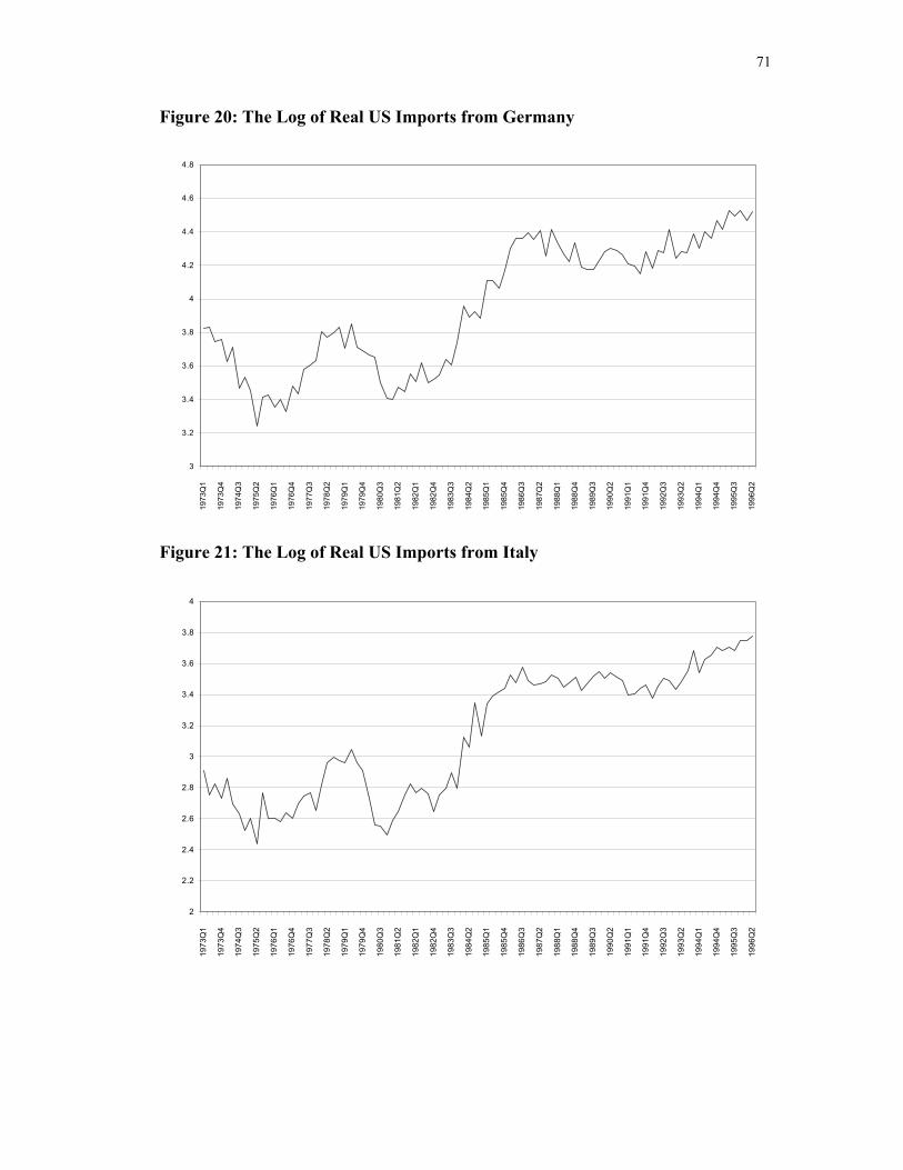
71
Figure 20: The Log of Real US Imports from Germany
Figure 21: The Log of Real US Imports from Italy
3
3.2
3.4
3.6
3.8
4
4.2
4.4
4.6
4.8
1973
Q1
1973
Q4
1974
Q3
1975
Q2
1976
Q1
1976
Q4
1977
Q3
1978
Q2
1979
Q1
1979
Q4
1980
Q3
1981
Q2
1982
Q1
1982
Q4
1983
Q3
1984
Q2
1985
Q1
1985
Q4
1986
Q3
1987
Q2
1988
Q1
1988
Q4
1989
Q3
1990
Q2
1991
Q1
1991
Q4
1992
Q3
1993
Q2
1994
Q1
1994
Q4
1995
Q3
1996
Q2
2
2.2
2.4
2.6
2.8
3
3.2
3.4
3.6
3.8
4
1973
Q1
1973
Q4
1974
Q3
1975
Q2
1976
Q1
1976
Q4
1977
Q3
1978
Q2
1979
Q1
1979
Q4
1980
Q3
1981
Q2
1982
Q1
1982
Q4
1983
Q3
1984
Q2
1985
Q1
1985
Q4
1986
Q3
1987
Q2
1988
Q1
1988
Q4
1989
Q3
1990
Q2
1991
Q1
1991
Q4
1992
Q3
1993
Q2
1994
Q1
1994
Q4
1995
Q3
1996
Q2

72
Figure 22: The Log of Real US Imports from Japan
Figure 23: The Log of Real US Imports from U.K.
3
3.5
4
4.5
5
5.5
6
1973
Q1
1973
Q4
1974
Q3
1975
Q2
1976
Q1
1976
Q4
1977
Q3
1978
Q2
1979
Q1
1979
Q4
1980
Q3
1981
Q2
1982
Q1
1982
Q4
1983
Q3
1984
Q2
1985
Q1
1985
Q4
1986
Q3
1987
Q2
1988
Q1
1988
Q4
1989
Q3
1990
Q2
1991
Q1
1991
Q4
1992
Q3
1993
Q2
1994
Q1
1994
Q4
1995
Q3
1996
Q2
2.5
2.7
2.9
3.1
3.3
3.5
3.7
3.9
4.1
4.3
4.5
1973
Q1
1973
Q4
1974
Q3
1975
Q2
1976
Q1
1976
Q4
1977
Q3
1978
Q2
1979
Q1
1979
Q4
1980
Q3
1981
Q2
1982
Q1
1982
Q4
1983
Q3
1984
Q2
1985
Q1
1985
Q4
1986
Q3
1987
Q2
1988
Q1
1988
Q4
1989
Q3
1990
Q2
1991
Q1
1991
Q4
1992
Q3
1993
Q2
1994
Q1
1994
Q4
1995
Q3
1996
Q2

73
Figure 24: The Log of the Real U.S. Bilateral Exchange Rate with Canada
Figure 25: The Log of the Real U.S. Bilateral Exchange Rate with France
4.2
4.3
4.4
4.5
4.6
4.7
4.8
4.9
1973
Q1
1973
Q4
1974
Q3
1975
Q2
1976
Q1
1976
Q4
1977
Q3
1978
Q2
1979
Q1
1979
Q4
1980
Q3
1981
Q2
1982
Q1
1982
Q4
1983
Q3
1984
Q2
1985
Q1
1985
Q4
1986
Q3
1987
Q2
1988
Q1
1988
Q4
1989
Q3
1990
Q2
1991
Q1
1991
Q4
1992
Q3
1993
Q2
1994
Q1
1994
Q4
1995
Q3
1996
Q2
4
4.2
4.4
4.6
4.8
5
5.2
5.4
1973
Q1
1973
Q4
1974
Q3
1975
Q2
1976
Q1
1976
Q4
1977
Q3
1978
Q2
1979
Q1
1979
Q4
1980
Q3
1981
Q2
1982
Q1
1982
Q4
1983
Q3
1984
Q2
1985
Q1
1985
Q4
1986
Q3
1987
Q2
1988
Q1
1988
Q4
1989
Q3
1990
Q2
1991
Q1
1991
Q4
1992
Q3
1993
Q2
1994
Q1
1994
Q4
1995
Q3
1996
Q2

74
Figure 26: The Log of the Real U.S. Bilateral Exchange Rate with Germany
Figure 27: The Log of the Real U.S. Bilateral Exchange Rate with Italy
4
4.2
4.4
4.6
4.8
5
5.2
5.4
1973
Q1
1973
Q4
1974
Q3
1975
Q2
1976
Q1
1976
Q4
1977
Q3
1978
Q2
1979
Q1
1979
Q4
1980
Q3
1981
Q2
1982
Q1
1982
Q4
1983
Q3
1984
Q2
1985
Q1
1985
Q4
1986
Q3
1987
Q2
1988
Q1
1988
Q4
1989
Q3
1990
Q2
1991
Q1
1991
Q4
1992
Q3
1993
Q2
1994
Q1
1994
Q4
1995
Q3
1996
Q2
4
4.2
4.4
4.6
4.8
5
5.2
5.4
1973
Q1
1973
Q4
1974
Q3
1975
Q2
1976
Q1
1976
Q4
1977
Q3
1978
Q2
1979
Q1
1979
Q4
1980
Q3
1981
Q2
1982
Q1
1982
Q4
1983
Q3
1984
Q2
1985
Q1
1985
Q4
1986
Q3
1987
Q2
1988
Q1
1988
Q4
1989
Q3
1990
Q2
1991
Q1
1991
Q4
1992
Q3
1993
Q2
1994
Q1
1994
Q4
1995
Q3
1996
Q2

75
Figure 28: The Log of the Real U.S. Bilateral Exchange Rate with Japan
Figure 29: The Log of the Real U.S. Bilateral Exchange Rate with UK
4
4.2
4.4
4.6
4.8
5
5.2
1973
Q1
1973
Q4
1974
Q3
1975
Q2
1976
Q1
1976
Q4
1977
Q3
1978
Q2
1979
Q1
1979
Q4
1980
Q3
1981
Q2
1982
Q1
1982
Q4
1983
Q3
1984
Q2
1985
Q1
1985
Q4
1986
Q3
1987
Q2
1988
Q1
1988
Q4
1989
Q3
1990
Q2
1991
Q1
1991
Q4
1992
Q3
1993
Q2
1994
Q1
1994
Q4
1995
Q3
1996
Q2
4
4.2
4.4
4.6
4.8
5
5.2
1973
Q1
1973
Q4
1974
Q3
1975
Q2
1976
Q1
1976
Q4
1977
Q3
1978
Q2
1979
Q1
1979
Q4
1980
Q3
1981
Q2
1982
Q1
1982
Q4
1983
Q3
1984
Q2
1985
Q1
1985
Q4
1986
Q3
1987
Q2
1988
Q1
1988
Q4
1989
Q3
1990
Q2
1991
Q1
1991
Q4
1992
Q3
1993
Q2
1994
Q1
1994
Q4
1995
Q3
1996
Q2

76
Figure 30: CUSUM Test for Export Demand with Canada
Figure 31: CUSUMSQ Test for Export Demand with Canada

77
Figure 32: CUSUM Test for Import Demand with Canada
Figure 33: CUSUMSQ Test for Import Demand with Canada

78
Figure 34: CUSUM Test for Export Demand with France
Figure 35: CUSUMSQ Test for Export Demand with France

79
Figure 36: CUSUM Test for Import Demand with France
Figure 37: CUSUMSQ Test for Import Demand with France

80
Figure 38: CUSUM Test for Export Demand with Germany
Figure 39: CUSUMSQ Test for Export Demand with Germany

81
Figure 40: CUSUM Test for Import Demand with Germany
Figure 41: CUSUMSQ Test for Import Demand with Germany

82
Figure 42: CUSUM Test for Export Demand with Italy
Figure 43: CUSUMSQ Test for Export Demand with Italy

83
Figure 44: CUSUM Test for Import Demand with Italy
Figure 45: CUSUMSQ Test for Import Demand with Italy

84
Figure 46: CUSUM Test for Export Demand with Japan
Figure 47: CUSUMSQ Test for Export Demand with Japan

85
Figure 48: CUSUM Test for Import Demand with Japan
Figure 49: CUSUMSQ Test for Import Demand with Japan

86
Figure 50: CUSUM Test for Export Demand with U.K.
Figure 51: CUSUMSQ Test for Export Demand with U.K.

87
Figure 52: CUSUM Test for Import Demand with U.K.
Figure 53: CUSUMSQ Test for Import Demand with U.K.

88
REFERENCES
Appleyard, Dennis R., and Alfred J. Field, Jr., “A Note on Teaching the Marshall- Lerner Condition,” Journal of Economic Education, (Winter 1986), 52-56.
Arize, Augustine C., “Cointegration Test of a Long-Run Relation Between the Real
Effective Exchange Rate and the Trade Balance,” International Economic Journal, Vol. 8, Autumn 1994, 1-9.
Bahmani-Oskooee, Mohsen, “Cointegration Approach to Estimate the long-Run Trade Elasticities in LDCs,” International Economic Journal, Vol. 12 (1998a), 89-96.
Bahmani-Oskooee, Mohsen, “Do Exchange Rates Follow a Random Walk in Middle
East Countries?” Economics Letters, Vol. 58 (1998b), 339-344.
Bahmani-Oskooee, Mohsen, “The Long-Run Determinants of the U.S. Trade Balance Revisited,” Journal of Post Keynesian Economics, Vol. 17 (Spring 1995), pp. 457-465. Bahmani-Oskooee, Mohsen, “More Evidence on the J-Curve from LDCs,” Journal of
Policy Modeling, Vol. 14, 1992, 641-653.
Bahmani-Oskooee, Mohsen, “Is there a Long-Run Relation between the Trade Balance and the Real Effective Exchange Rate of LDCs?” Economics Letters, Vol. 36 1991, 403-407.
Bahmani-Oskooee, Mohsen, “Determinants of International Trade Flows: The case of Developing Countries,” Journal of Development Economics, Vol. 20, January- February 1986, 107-123. Bahmani-Oskooee, Mohsen, “Devaluation and the J-Curve: Some Evidence from
LDCs,” Review of Economics and Statistics, Vol. 67, 1985, 500-504.
Barker, Terry S., and M. Hashem Pesaran, “Disaggregation in Econometric Modelling: An Introduction,” in Disaggreagation in Econometric Modelling, eds. T.S. Barker and M.H. Pesaran, (1990).
Bickerdike, Charles F., “The Theory of Incipient Taxes,” Economic Journal, Vol.16
December (1906), 529-535.
Bickerdike, Charles F., “The Instability of Foreign Exchange,” Economic Journal, Vol 30 March (1920), 118-122.
Brown, R.L., J Durbin and J.M. Evans, “Techniques for Testing the Constancy of

89
Regression Relationships over Time,” Journal of the Royal Statistical Society B, Vol. 35, 1975, 149-192.
Carone, Giuseppe. “Modeling th U.S. Demand for Imports through Cointegration and Error Correction.” Journal of Policy Modeling, vol. 18, no.1 (February 1996),
1-48. Cheung, Yin-Wong, and Menzie David Chinn, “Deterministic, Stochastic, and Segmented Trend in Aggregate Output: A Cross-Country Analysis,” Oxford Economics Papers, Forthcoming. Cheung, Yin-Wong, and Kon S. Lai, “Finite-Sample Sizes of Johansen’s Likelihood Ratio Tests for Cointegration,” Oxford Bulletin of Economics and Statistics,
Vol. 55 (1993), 313-328. Chipman, John S., “Bikerdike’s Theory of Incipient and Optimal Tariffs,” History of
Political Economy, Vol. 25 no. 3, (1993), 461-491. Chipman, John S., “Bickerdike, Charles F.,” in The New Palgrave: A Dictionary of
Economics, Ed. Eatwell et al. Vol 3, (1987) 237-238. Cushman, David O., “U.S. Bilateral Trade Balances and the Dollar,” Economics
Letters, Vol. 24, 1987, 363-367. Deyak, Timothy A., W. Charles Sawyer and Richard L. Sprinkle, “An Empirical
Examination of the Structural Stability of Disaggregated U.S. Import Demand: Note,” Review of Economics and Statistics, Vol. , (1989), 337-341.
Dickey, D. A. and Fuller, W.A.. "Distribution of the Estimators for Autoregressive
Time Series with a Unit Root," Journal of the American Statistical Association, Vol. 74, (1979), 427-431.
Dornbusch, R., Open Economy Macroeconomics, (Basic Books, 1980). Goldstein, Morris, and Mohsin S. Khan, “Income and Price Effects in Foreign
Trade,” in: R.W. Jones and P.B. Kenen, eds., Handbook of International Economics, (North-Holland, Amsterdam), 1041-1105.
Granger, Clive W. J. and P. Newbold, “Spurious Regressions in Econometrics,”
Journal of Econometrics, Vol. 2, (1974), 111-120. Hickman, Bert G., and Lawrence J. Lau, “Elasticities of Substitution and Export
Demands in a World Trade Model,” European Economic Review, Vol. 4, (1973), 347-380.

90
Houthakker, Hendrik S. and Stephen Magee, “Income and Price Elasticities in World Trade,” Review of Economics and Statistics, Vol. 51, May 1969, 111-125. Hooper, Peter and Jaime Marquez, “Exchange Rates, Prices and External Adjustment
in the United States, in P. Kenen, ed., Understanding Interdependence, Princeton N.J.: Princenton University Press, (1995), 107-168.
Johansen, Soren and Katerina Juselius, Maximum Likelihood Estimation and Inference on Cointegration-With Application to the Demand for Money,” Oxford Bulletin of Economics snd Statistics, Vol. 52, May 1990, 169-210.
Khan, Mohsin, “Import and Export Demand in Developing Countries,” IMF Staff
Papers, Vol. 21, September1974, 678-693. King, Robert G., Charles I. Plosser, James H. Stock, and Mark W. Watson,
"Stochastic Trends and Economic Fluctuations", American Economic Review, September 1991, 819-840.
Kreinin, Mordechai E., “Price Elasticities in the International Trade,” Review of Economics and Statistics, Vol. 49, November 1967, 510-516. Kwiatkowski, Denis; Peter C.B. Phillips; Peter Schmidt and Yongcheol Shin,
“Testing the Null Hypothesis of Stationarity against the Alternative of a Unit Root,” Journal of Econometrics, Vol. 54 (1992), 159-178.
Leamer, Edward E., and Robert M. Stern, Quantitative International Economics,
Allyn and Bacon, 1970. Lerner, Abba P., The Economics of Control, New York: Macmillan, (1944). Lindert, P. H. and T.A. Pugel, International Economics, (Irwin, 10th Edition). MacKinnon, "Critical Values for Cointegration Tests," Chapter 13 in eds. R.F. Engel
and C.W.J. Granger, Long-Run Economic Relationships: Readings in Cointegration, (1991).
Marquez, Jaime, “Bilateral Trade Elasticities,” Review of Economics and Statistics, Vol. 72, February 1990, 70-77. Marquez, Jaime, “The Dynamics of Uncertainty or the Uncertainty of Dynamics: Stochastic J-Curves,” Review of Economics and Statistics, Vol 73, 125-133. Marwah, Kanta and Lawrence R. Klein, “Estimation of J-Curves: United Staes and
Canada,” Canadian Journal of Economics, Vol. 19 no. 3, August 1996, 523-539.

91
Moffett, Michael H., "The J-Curve Revisitied: An Empirical Examination for the United States," Journal of International Money and Finance, Vol. 8, (1989), 425-444.
Nelson, Charles R. and Charles I. Plosser, “Trends and Random Walks in Macroeconomic Time Series,” Journal of Monetary Economics, (1982), 129- 162.
Orcutt, Guy H., “Measurement of Price Elasticities in International Trade,” Review
of Economics and Statistics, Vol. 32 no.20, (1950), 117-132. Pedroni, Peter, “Fully Modified OLS for Heterogenous Cointegrated Panels and the
Case of Purchasing Power Parity,” Indiana University Working Papers in Economics, No.96-020. (1996).
Pedroni, Peter, “Testing for Convergence to Common Steady States in Nonstationary Heterogeneous Panels,” Indiana University Working Papers in Economics, (1998).
Phillips, P.C.B., “Understanding Spurious Regressions,” Journal of Economterics, Vol. 33, (1986), 311-340.
Phillips, Peter and Bruce Hansen, “Statistical Inference in Instrumental Variables
Regression with I(1) Processes,” Review of Economic Studies, Vol. 57, (1990), 99-125.
Pierse, Richard and A.J. Snell “Temporal Aggregation and the Power of Tests for a
Unit Root,” Journal of Econometrics, Vol. 65, (February 1995), 333-345. Resnick, Stephen A., and Edwin M. Truman, “An Empirical Examination of Bilateral
Trade in Western Europe,” Journal of International Economics, Vol. 3, (1973), 305-335.
Rose, Andrew K., “The Role of Exchange Rates in a Popular Model of International
Trade: Does the ‘Marshall-Lerner’ Condition Hold?” Journal of International Economics, Vol. 30, (1991), 301-316.
Rose, Andrew K. and Janet L. Yellen, “Is There a J-Curve?” Journal of Monetary Economics, Vol. 24, (1989), 53-68. Sawyer, Charles W., and Richard L. Sprinkle, “The Demand for Imports and Exports
in the U.S.: A Survey,” Journal of Economics and Finance, Vol. 20 no.1, (Spring 1996), 147-178.
Shiller, Robert and Pierre Perron, “Testing the Random Walk Hypothesis: Power vs.
Frequency of Observation,” NBER Technical Paper: 45, April (1985).

92
Shirvani, Hassan and Barry Wilbratte, “The Relationship Between the Real Exchange
Rate and the Trade Balance: An Empirical Reassessment,” International Economic Journal, Vol. 11. no. 1, (Spring 1997), 39-50.
Stern, Robert M., The Balance of Payments, (Aldine Publishing Company, 1973). Stern, Robert M., Jonathan Francis and Bruce Schumacher, Price Elasticities in
International Trade: An Annotated Bibliography, (London, Macmillan, 1976).
Toda, H. Y., “Finite Sample Properties of Likelihood Ratio Tests for Cointegrating Ranks when Linear Trends are Present,” Review of Economics and Statistics, Vol. 76 (1994), 66-79.
Tower, Edward, “Separability: The One Principal and Serious Defect of Bikerdike’s
and Edgeworth’s Elasticity Approach to Balance-of-Payments Problems?” History of Political Economy, Vol. 25 no. 3, (1993), 492-497.
Zietz, Joachim, and Donald K. Pemberton, “Parameter Instability in Aggregate US
Import Demand Functions,” Journal of International Money and Finance, Vol. 12, (1993), 654-667.

93
Appendix A: Mathematical Derivation of the Marshall-Lerner Condition.
The following derivation follows from Stern (1973). The trade balance in
foreign currency terms is:
MpXpB fmfxf −≡ (A.1)
The change in the trade balance after a depreciation can be denoted as:
)()( fmfmfxfxf pMMppXXpB ∆+∆−∆+∆≡∆ (A.2)
If we indicate the initial value of export and imports as follows:
XpV fxfx ≡ Foreign value of exports (A.3)
MpV fmfm ≡ Foreign value of imports (A.4)
Then rearranging terms and substituting (A.3) and (A.4) into (A.2) yields:
∆−
∆−+
∆+
∆≡∆
fm
fmfm
fx
fxfxf p
pMMV
pp
XXVB (A.5)
The elasticities of demand and supply of exports and imports are defined below. Note
that traditionally negative demand elasticities are expressed so as to enter in
positively into the expression.
hx
hxx p
pXXe ∆∆
≡ Home export supply elasticity (A.6)
fx
fxx p
pXX ∆∆
−≡η Foreign export demand elasticity (A.7)
fm
fmm p
pMMe
∆∆≡ Foreign import supply elasticity (A.8)
hm
hmm p
pMM ∆∆
−≡η Home import demand elasticity (A.9)
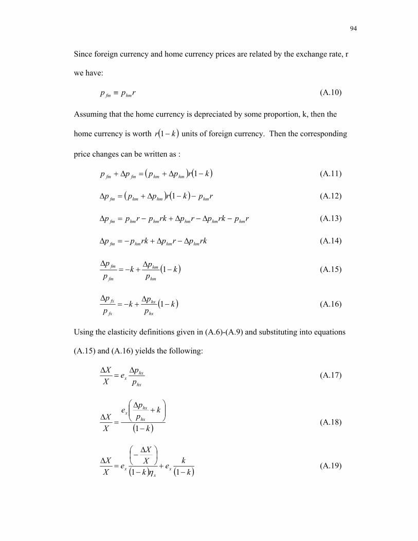
94
Since foreign currency and home currency prices are related by the exchange rate, r
we have:
rpp hmfm ≡ (A.10)
Assuming that the home currency is depreciated by some proportion, k, then the
home currency is worth ( )kr −1 units of foreign currency. Then the corresponding
price changes can be written as :
( ) ( )krpppp hmhmfmfm −∆+=∆+ 1 (A.11)
( ) ( ) rpkrppp hmhmhmfm −−∆+=∆ 1 (A.12)
rprkprprkprpp hmhmhmhmhmfm −∆−∆+−=∆ (A.13)
rkprprkpp hmhmhmfm ∆−∆+−=∆ (A.14)
( )kppk
pp
hm
hm
fm
fm −∆
+−=∆
1 (A.15)
( )kppk
pp
hx
hx
fx
fx −∆
+−=∆
1 (A.16)
Using the elasticity definitions given in (A.6)-(A.9) and substituting into equations
(A.15) and (A.16) yields the following:
hx
hxx p
peXX ∆
=∆ (A.17)
( )k
kppe
XX hx
hxx
−
+
∆
=∆
1 (A.18)
( ) ( )kke
kXX
eXX
xx
x −+
−
∆
−=
∆11 η
(A.19)

95
( )
( ) x
x
x
ke
kke
XX
η−+
−=∆
11
1 (A.20)
( ) xx
xx
keke
XX
ηη−+
=∆
1 (A.21)
( ) xx
x
fx
fx
keke
pp
η−+−=
∆
1 (A.22)
( )keke
MM
mm
mm
−+=
∆1η
η (A.23)
( )kek
pp
mm
m
fm
fm
−+=
∆
1ηη (A.24)
Substituting equations (A.21)-(A.24) into equation (A.5) expresses the change in the
foreign currency value of the trade balance in terms of demand and supply elasticities.
( )( )
( )( )
−+
++
−+−
=∆ke
eVke
eVkBmm
mmfm
xx
xxfxf 1
11
1η
ηηη
(A.25)
assuming that the proportion of the depreciation, k is small then:
( )( )[ ]
( ) 111
11
++
++
−=∆
mm
mmfm
xx
xfxf e
eV
eVB
ηη
ηη
(A.26)
I. This is generally referred to as the Bickerdike-Robinson-Metzler
condition, herein (BRM). If prices are fixed in seller's currencies, then
the supply elasticities are infinitely elastic, which is expressed in equation
(A.27).
∞== mx ee (A.27)
Then we have:

96
( ) ( )mfmxfxf VVB ηη +−=∆ 1 (A.28)
Furthermore if we assume that trade was initially balanced so that the foreign
currency value of exports equals the foreign currency value of imports then we have
equation (A.29).
1=fmfx VV (A.29)
Then the foreign currency value of the trade balance improves
0>∆ fB (A.30)
if the sum of the import and export demand elasticities is greater than unity
1>+ mx ηη (A.31)
This is known generally as the Marshall-Lerner condition, herein (M-L). It may be of
additional value if the assumption of initially balanced trade, made in equation
(A.29), is relaxed. First we will consider the case where the trade balance is in
surplus. So:
1>fmfx VV (A.32)
Then the foreign currency value of the trade balance improves
0>∆ fB (A.33)
if the sum of the export demand elasticity and the "weighted" import demand
elasticity are greater than unity, where the weight is the foreign currency value of
imports divided by the foreign currency value of exports.
1>+ mfx
fmx V
Vηη (A.34)
97
It can be seen that when the trade balance is in surplus the M-L condition is no longer
a sufficient condition. If we turn to the final case where there is a trade deficit
initially, we have:
1<fmfx VV (A.35)
then:
0>∆ fB (A.36)
if
1>+ mfx
fmx V
Vηη (A.34)
Now the M-L condition becomes a sufficient and not a necessary condition, as the
"weighted" import demand elasticity can be much smaller and still insure an
improvement in the trade balance. This is one explanation for the different findings
in the J-curve literature. The M-L condition is more stringent then necessary to
insure a depreciation improves the trade balance.

98
Appendix B: Data Sources
All data are quarterly covering the period from 1973:I - 1996:II. The log of
real GDP for the US is usLY , and it has been converted to index form where the base
is 1990:I. The log of real GDP for each of the remaining countries is iLY where i
denotes the country. These variables are also in index form with the base year 1990:I.
The data, except Germany's real GDP, come from International Financial Statistics
of the International Monetary Fund, CD- ROM. The GDP data for Germany come
from the OECD Economic Indicators.
The real bilateral exchange rate, iLREX , is the log of the average nominal
exchange in country i’s currency units per dollar, multiplied by the ratio of the US
GDP deflator to country i’s GDP deflator. The GDP deflators are calculated from the
nominal and real GDP's for each country found in the International Financial
Statistics CD-ROM. The nominal bilateral exchange rate, is the average spot rate for
the quarter, as reported in the IFS CD-ROM.
The log of US imports, iLM , is the log of nominal US imports from country i
divided by the unit value price index of imports for the US. Similarly the log of US
exports, iLX , is the log of nominal exports to country i divided by the unit value
price index of exports for the US. The unit value price indices come from the IFS
CD-ROM, and the trade data come from the Direction of Trade Statistics of
the International Monetary Fund, various issues.
There are several sources of concern or rather caution about the data. One
source involves the unit value index for imports and exports used to deflate the
nominal trade. They potentially introduce a source of error since these indices are

99
calculated based on aggregate trade and not bilateral trade. If bilateral trade is
commodity specific, we might not accurately be capturing real quantity changes when
deflating the nominal data. Leamer and Stern (1970) also point to the potential
problems when using unit value indices rather then price indices.
100
VITA Title of Dissertation Currency Devaluation and the Trade Balance: An Elasticity Approach to Test the Marshall-Lerner Condition for Bilateral Trade Between the US and the G-7. Full Name Taggert J. Brooks Place of Birth Milwaukee, WI Colleges and Universities Ph.D., Economics, University of Wisconsin-Milwaukee, September 1996-May 1999 M.A., Economics, University of Wisconsin-Milwaukee, September 1994-May 1996 B.A., Economics, University of Wisconsin-Madison, September 1993-May 1993 Memberships in Learned or Honorary Societies American Economic Association Midwest Economic Association Transportation Research Forum. Publications "Bilateral J-Curve Between the U.S. and her Trading Partners." with Mohsen Bahmani-Oskooee, Weltwirtshaftliches Archiv, Forthcoming. "A Cointegration Approach to Estimating the Bilateral Trade Elasticities Between the U.S. and Her Trading Partners." with Mohsen Bahmani-Oskooee, International Economic Journal, Forthcoming. Major Department Economics Signed____________________________________________________________ Major Professor in charge of Dissertation


