CS/EE 5590 / ENG 401 Multimedia Communication, Spring 2017
Lec 06
Transforms and Quantization I
Zhu Li
Course Web:
http://l.web.umkc.edu/lizhu/
Z. Li, Multimedia Communciation, Spring 2017 p.1

Outline
Lecture 05 Arithmetic Coding Re-Cap
Signal Transform
KLT/PCA
DCT
Z. Li, Multimedia Communciation, Spring 2017 p.2
Arithmetic Coding ReCAp
Arithmetic coding:
Symbols A={a1, a2, …, an}, with prob={p1, p2, …, pn}
For a sequence of symbol, X=[x1, x2, …, xm] compute the sequence prob, P(X), the binary code is,
of the F(X) representation.
Sequence prob based, more efficient than Huffman codes
Z. Li, Multimedia Communciation, Spring 2017 p.3
Aliens visit earth….
bits. 1)(
1log)(
XpXl
Example - Arithmetic
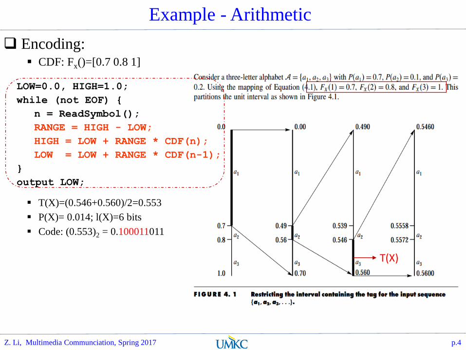
Encoding: CDF: Fx()=[0.7 0.8 1]
T(X)=(0.546+0.560)/2=0.553
P(X)= 0.014; l(X)=6 bits
Code: (0.553)2 = 0.100011011
Z. Li, Multimedia Communciation, Spring 2017 p.4
LOW=0.0, HIGH=1.0;
while (not EOF) {
n = ReadSymbol();
RANGE = HIGH - LOW;
HIGH = LOW + RANGE * CDF(n);
LOW = LOW + RANGE * CDF(n-1);
}
output LOW;
T(X)
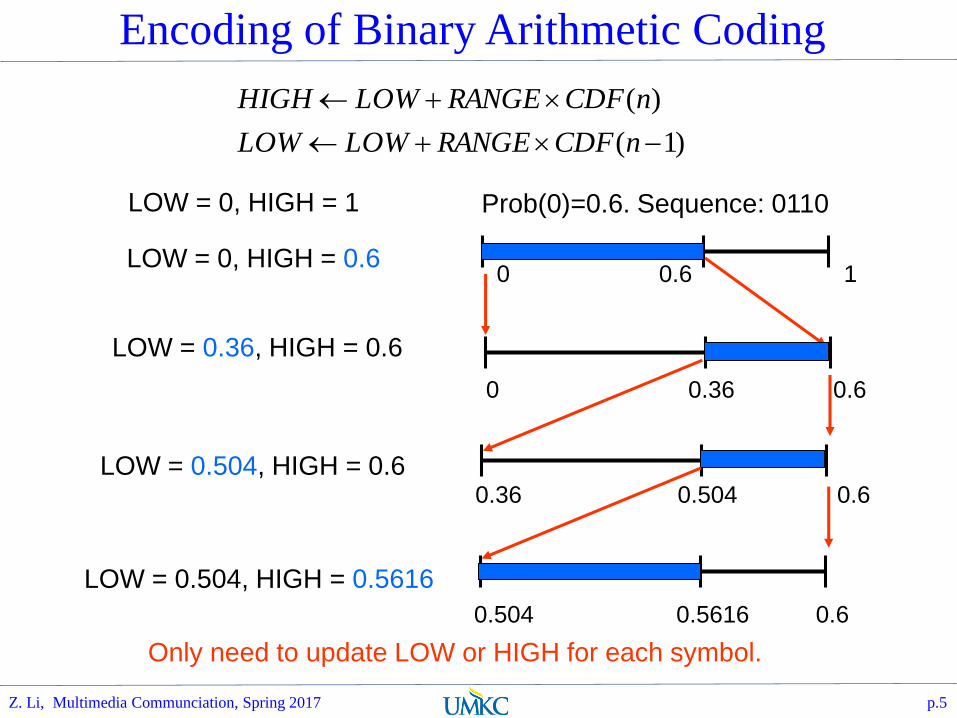
Encoding of Binary Arithmetic Coding
Prob(0)=0.6. Sequence: 0110LOW = 0, HIGH = 1
0 0.6 1LOW = 0, HIGH = 0.6
0 0.36 0.6
LOW = 0.36, HIGH = 0.6
0.36 0.504 0.6LOW = 0.504, HIGH = 0.6
0.504 0.5616 0.6
LOW = 0.504, HIGH = 0.5616
Only need to update LOW or HIGH for each symbol.
)1(
)(
nCDFRANGELOWLOW
nCDFRANGELOWHIGH
Z. Li, Multimedia Communciation, Spring 2017 p.5

Adaptive Arithmetic Coding
Observation:
The partition of [0, 1) can be different from symbol to symbol
The bit stream can be decoded perfectly as long as both encoder and decoder are synchronized (use the same probability).
Only need to update the probabilities
Adaptive Huffman code:
Has to redesign the codebook each time
Time-consuming.
Binary arithmetic
EncoderX(n)
p0(n)
Binary arithmetic
Decoder
p0(n)
X(n)bitstream
Z. Li, Multimedia Communciation, Spring 2017 p.6

Example
0 0.5 1
Binary sequence: 01111
Initial counters for 0’s and 1’s:
C(0)=C(1)=1.
P(0)=P(1)=0.5
0 0.3333 0.5 After encoding 0: C(0)=2, C(1)=1.
P(0)=2/3, P(1)=1/3
0.3333 0.4167 0.5 After encoding 01: C(0)=2, C(1)=2.
P(0)=1/2, P(1)=1/2
0.4167 0.45 0.5 After encoding 011: C(0)=2, C(1)=3.
P(0)=2/5, P(1)=3/5
0.45 0.4667 0.5 After encoding 0111: C(0)=2, C(1)=4.
P(0)=1/3, P(1)=2/3.
Encode 0.4667.
Z. Li, Multimedia Communciation, Spring 2017 p.7

Decoding
Input 0.4667.
Initial counters for 0’s and 1’s:
C(0)=C(1)=1 P(0)=P(1)=0.5
Decode 0
0 0.5 1
0 0.3333 0.5 After decoding 0: C(0)=2, C(1)=1.
P(0)=2/3, P(1)=1/3
Decode 1
After decoding 01: C(0)=2, C(1)=2.
P(0)=1/2, P(1)=1/2
Decode 1
0.3333 0.4167 0.5
After decoding 011: C(0)=2, C(1)=3.
P(0)=2/5, P(1)=3/5
Decode 1
0.4167 0.45 0.5
After decoding 0111: C(0)=2, C(1)=4.
P(0)=1/3, P(1)=2/3.
Decode 1
0.45 0.4667 0.5
Z. Li, Multimedia Communciation, Spring 2017 p.8

Context-adaptive Arithmetic Coding
In many cases, a sample has strong correlation with its near neighbors.
Idea:
Collect conditional probability distribution of a symbol for given neighboring symbols (context):
P(x(n) | x(n-1), x(n-2), … x(n-k))
Use this conditional probability to encode the next symbol
More skewed probability distribution can be obtained (desired for arithmetic coding)
a b c b c a b
1-D
Context
template
a b c b c a b
c b a b c b a2-D
Context
template
Z. Li, Multimedia Communciation, Spring 2017 p.9
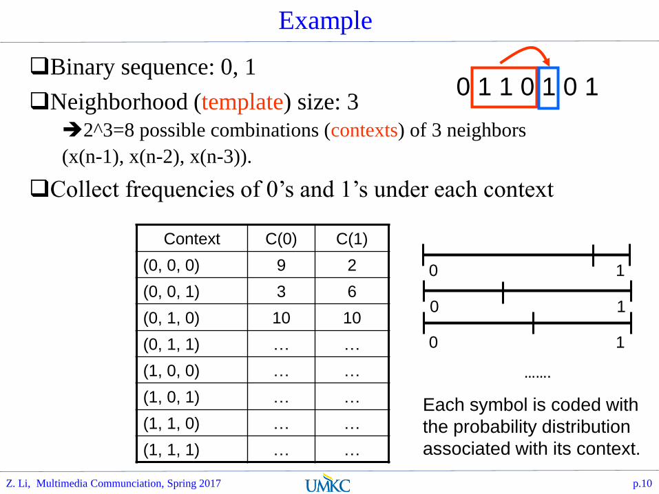
Example
Binary sequence: 0, 1
Neighborhood (template) size: 3
2^3=8 possible combinations (contexts) of 3 neighbors
(x(n-1), x(n-2), x(n-3)).
Collect frequencies of 0’s and 1’s under each context
0 1 1 0 1 0 1
Context C(0) C(1)
(0, 0, 0) 9 2
(0, 0, 1) 3 6
(0, 1, 0) 10 10
(0, 1, 1) … …
(1, 0, 0) … …
(1, 0, 1) … …
(1, 1, 0) … …
(1, 1, 1) … …
0 1
0 1
0 1
Each symbol is coded with
the probability distribution
associated with its context.
Z. Li, Multimedia Communciation, Spring 2017 p.10
…….

Modeling Large Context
Condition reduces entropy, H(Y|X1) > H(Y|X1, X2, ….)
How to model very large context (x1, x2, ….)? Use a (shallow/deep) neural network to model context
Large window of 552 input nodes
7 sets of 3080 hidden nodes
Potential project: deeper neural network for HEVC CABAC context modeling
Z. Li, Multimedia Communciation, Spring 2017 p.11
CABAC in H.264
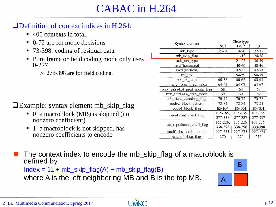
Definition of context indices in H.264:
400 contexts in total.
0-72 are for mode decisions
73-398: coding of residual data.
Pure frame or field coding mode only uses 0-277.
o 278-398 are for field coding.
Example: syntax element mb_skip_flag
0: a macroblock (MB) is skipped (no nonzero coefficient)
1: a macroblock is not skipped, has nonzero coefficients to encode
The context index to encode the mb_skip_flag of a macroblock is defined byIndex = 11 + mb_skip_flag(A) + mb_skip_flag(B)
where A is the left neighboring MB and B is the top MB. A
B
Z. Li, Multimedia Communciation, Spring 2017 p.12

Coefficient Coding: HEVC vs H.264
Z. Li, Multimedia Communciation, Spring 2017 p.13
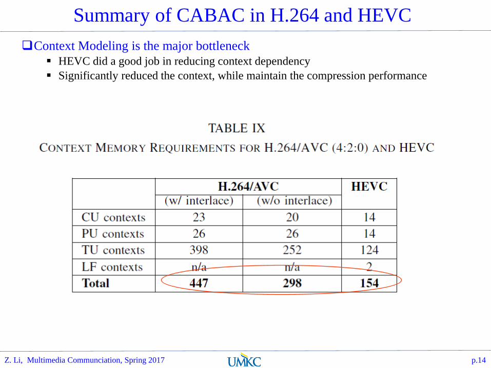
Summary of CABAC in H.264 and HEVC
Context Modeling is the major bottleneck
HEVC did a good job in reducing context dependency
Significantly reduced the context, while maintain the compression performance
Z. Li, Multimedia Communciation, Spring 2017 p.14
Outline
Lecture 05 Arithmetic Coding Re-Cap
Signal Transform
KLT/PCA
DCT
Z. Li, Multimedia Communciation, Spring 2017 p.15

Transform - Objective
Objective: to find alternative representation of the image/signal that is more compact
Z. Li, Multimedia Communciation, Spring 2017 p.16
*=
Quant Table:
*
8 24 -2 0 0 0 0 0
-31 -4 6 -1 0 0 0 0
0 -12 -1 2 0 0 0 0
0 0 -2 -1 0 0 0 0
0 0 0 0 0 0 0 0
0 0 0 0 0 0 0 0
0 0 0 0 0 0 0 0
0 0 0 0 0 0 0 0

Block Transform
Divide input data into blocks, encode each block separately
Matrix representation:
11 NNNN xTy TX y
Inverse Transform:
yTx1 TX
y
T x-1
Orthogonal (orthonormal) Transform:
TTT 1
TXy
T xT
Biorthogonal Transform: TTT 1
Z. Li, Multimedia Communciation, Spring 2017 p.17

Property of Orthogonal Transform
Txy T orthogonal.
22xy
1. Orthogonal transform preserves the energy:
Proof:
2 2T T T T y y y x T Tx x x x
Z. Li, Multimedia Communciation, Spring 2017 p.18

Property of Orthogonal Transform
Txy T orthogonal.
TXy
TT
e
x̂
22x̂xe
2. Orthogonal transform does not amplify the noise:
Proof:
2 2 2ˆthen x x v eLet ,Tv T e
Z. Li, Multimedia Communciation, Spring 2017 p.19
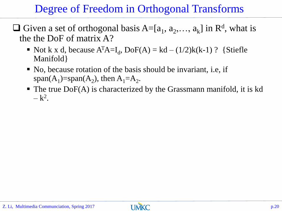
Degree of Freedom in Orthogonal Transforms
Given a set of orthogonal basis A=[a1, a2,…, ak] in Rd, what is the the DoF of matrix A?
Not k x d, because ATA=Id, DoF(A) = kd – (1/2)k(k-1) ? {StiefleManifold}
No, because rotation of the basis should be invariant, i.e, if span(A1)=span(A2), then A1=A2.
The true DoF(A) is characterized by the Grassmann manifold, it is kd– k2.
Z. Li, Multimedia Communciation, Spring 2017 p.20

Karhunen-Loéve Transform (KLT)
Also known as Hotelling transform, Principle Component method (energy preserving interpretation).
Goal: To decorrelate the input with an orthogonal transform:
T is orthogonal
We want uncorrelated diagonal.iy yyR
.T Txx yyR T T R
Rows of T should be the eigenvectors of Rxx.
the variances of {yi} should be the eigenvalues of Rxx.
1.
2.
.U TT
Recall: Eigen-decomposition: If A is square,
D: diagonal matrix with engenvalues on the diagonal.
U: columns are eigenvectors.
A symmetric U orthonormal
The KLT transform should be chosen as
.1UDUA
DAUU T
𝑦 = 𝑇𝑥, 𝑅𝑦𝑦 = 𝑦𝑦𝑇 𝑦𝑦𝑇 = 𝑇𝑥 𝑇𝑥 𝑇 = 𝑇 𝑥𝑥𝑇 𝑇𝑇 = 𝑇𝑅𝑥𝑥𝑇
𝑇
Z. Li, Multimedia Communciation, Spring 2017 p.21

Principal Component Analysis (PCA)
• Given: N data points x1, … ,xN in Rd
• We want to find a new set of features that are linear combinations of original ones:
u(xi) = uT(xi – µ)
• (µ: mean of data points)
• Choose unit vector u in Rd that captures the most data variance (max energy preservation)
Z. Li, Multimedia Communciation, Spring 2017 p.22
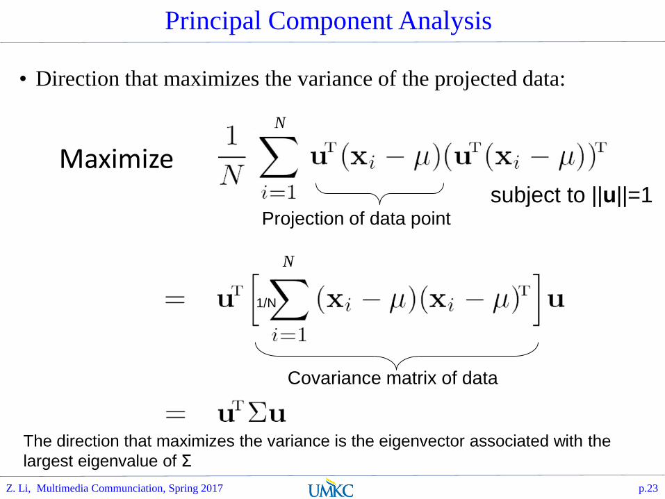
Principal Component Analysis
• Direction that maximizes the variance of the projected data:
Projection of data point
Covariance matrix of data
The direction that maximizes the variance is the eigenvector associated with the
largest eigenvalue of Σ
N
N
1/N
Maximizesubject to ||u||=1
Z. Li, Multimedia Communciation, Spring 2017 p.23
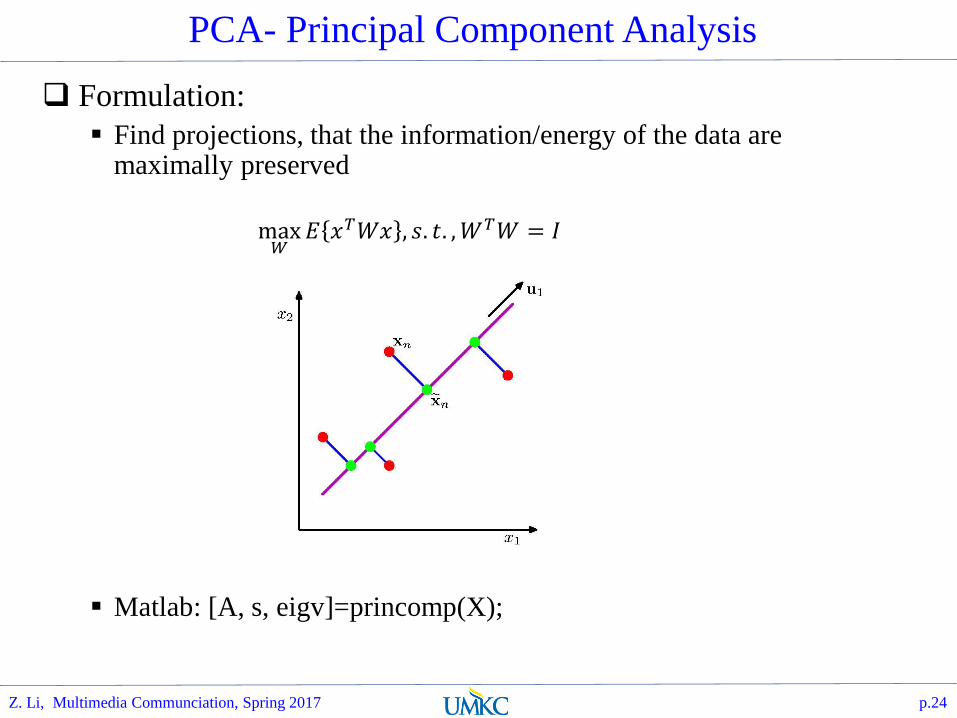
PCA- Principal Component Analysis
Formulation:
Find projections, that the information/energy of the data are maximally preserved
Matlab: [A, s, eigv]=princomp(X);
Z. Li, Multimedia Communciation, Spring 2017 p.24
max𝑊𝐸 𝑥𝑇𝑊𝑥 , 𝑠. 𝑡. ,𝑊𝑇𝑊 = 𝐼

PCA algorithm
PCA algorithm(X, k): top k eigenvalues/eigenvectors
% X = N m data matrix,
% … each data point xi = column vector, i=1..m
•
• X subtract mean x from each column vector xi in X
• XXT … covariance matrix of X
• { i, ui }i=1..N = eigenvectors/eigenvalues of
... 1 2 … N
• Return { i, ui }i=1..k% top k principle components
m
im 1
1ixx
Z. Li, Multimedia Communciation, Spring 2017 p.25

PCA Algorithm
Center the data:
X = X – repmat(mean(x), [n, 1]);
Principal component #1 points in the direction of the largest variance
Each subsequent principal component…
is orthogonal to the previous ones, and
points in the directions of the largest variance of the residual subspace
Solved by finding Eigen Vectors of the Scatter/Covarinace matrix of data:
S = cov(X); [A, eigv]=Eig(S)
Z. Li, Multimedia Communciation, Spring 2017 p.26
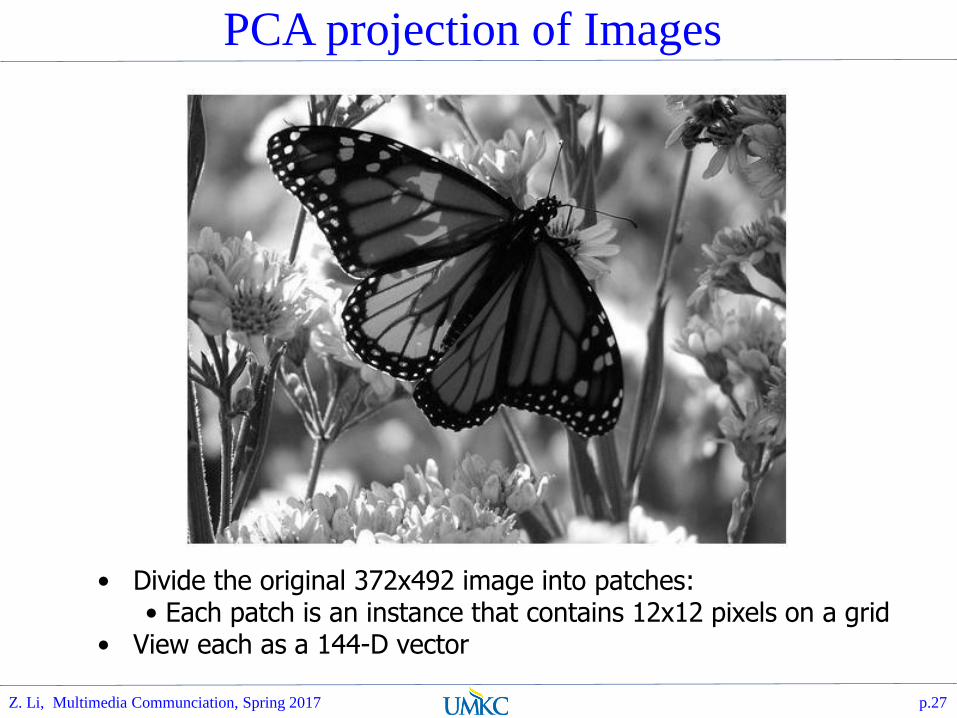
PCA projection of Images
• Divide the original 372x492 image into patches:• Each patch is an instance that contains 12x12 pixels on a grid
• View each as a 144-D vector
Z. Li, Multimedia Communciation, Spring 2017 p.27

Eigen Values (energy) and PCA dim
Z. Li, Multimedia Communciation, Spring 2017 p.28

PCA compression: kd=144 >> kd=60
Z. Li, Multimedia Communciation, Spring 2017 p.29

PCA compression: 144d > 16d
Z. Li, Multimedia Communciation, Spring 2017 p.30
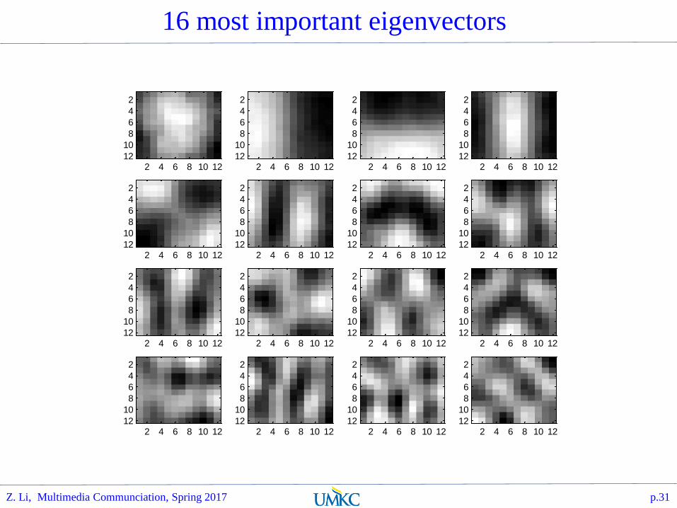
16 most important eigenvectors
2 4 6 8 10 12
2
4
6
8
10
122 4 6 8 10 12
2
4
6
8
10
122 4 6 8 10 12
2
4
6
8
10
122 4 6 8 10 12
2
4
6
8
10
12
2 4 6 8 10 12
2
4
6
8
10
122 4 6 8 10 12
2
4
6
8
10
122 4 6 8 10 12
2
4
6
8
10
122 4 6 8 10 12
2
4
6
8
10
12
2 4 6 8 10 12
2
4
6
8
10
122 4 6 8 10 12
2
4
6
8
10
122 4 6 8 10 12
2
4
6
8
10
122 4 6 8 10 12
2
4
6
8
10
12
2 4 6 8 10 12
2
4
6
8
10
122 4 6 8 10 12
2
4
6
8
10
122 4 6 8 10 12
2
4
6
8
10
122 4 6 8 10 12
2
4
6
8
10
12
Z. Li, Multimedia Communciation, Spring 2017 p.31
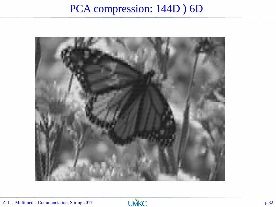
PCA compression: 144D ) 6D
Z. Li, Multimedia Communciation, Spring 2017 p.32

SVD
PCA: pull the n x m image blocks as vector in Rnxm.
The Singular Value Decomposition (SVD) of an nxm matrix A, is,
Where the diagonal of S are the eigen values of AAT, [𝜎1, 𝜎2, … , 𝜎𝑛]
U are eigenvectors of AAT, and V are eigen vectors of ATA, the outer product of uivi
T, are basis of A in reconstruction:
Z. Li, Multimedia Communciation, Spring 2017 p.33
𝐴 = 𝑈𝑆𝑉𝑇 =
𝑖
𝜎𝑖𝑢𝑖𝑣𝑖𝑡
A(mxn) = U(mxm) S(mxn)
V(nxn)
The 1st order SVD approx. of A is:
𝜎1 ∗ 𝑈 : , 1 ∗ 𝑉 : , 1𝑇
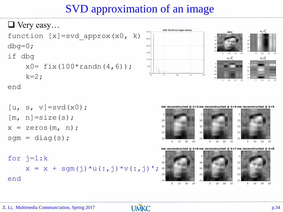
SVD approximation of an image
Very easy…
function [x]=svd_approx(x0, k)
dbg=0;
if dbg
x0= fix(100*randn(4,6));
k=2;
end
[u, s, v]=svd(x0);
[m, n]=size(s);
x = zeros(m, n);
sgm = diag(s);
for j=1:k
x = x + sgm(j)*u(:,j)*v(:,j)';
end
Z. Li, Multimedia Communciation, Spring 2017 p.34
Outline
Lecture 05 Arithmetic Coding Re-Cap
Signal Transform
KLT/PCA
DCT
Z. Li, Multimedia Communciation, Spring 2017 p.35

2-D Block Transform
Problem with SVD/PCA
Data dependent
Non-separable Transform
Separable approach:
Apply transform to each row, then to each column
T
NNNNNN NN TXTY
col tx row tx
Matrix form:
An N x N block
Z. Li, Multimedia Communciation, Spring 2017 p.36
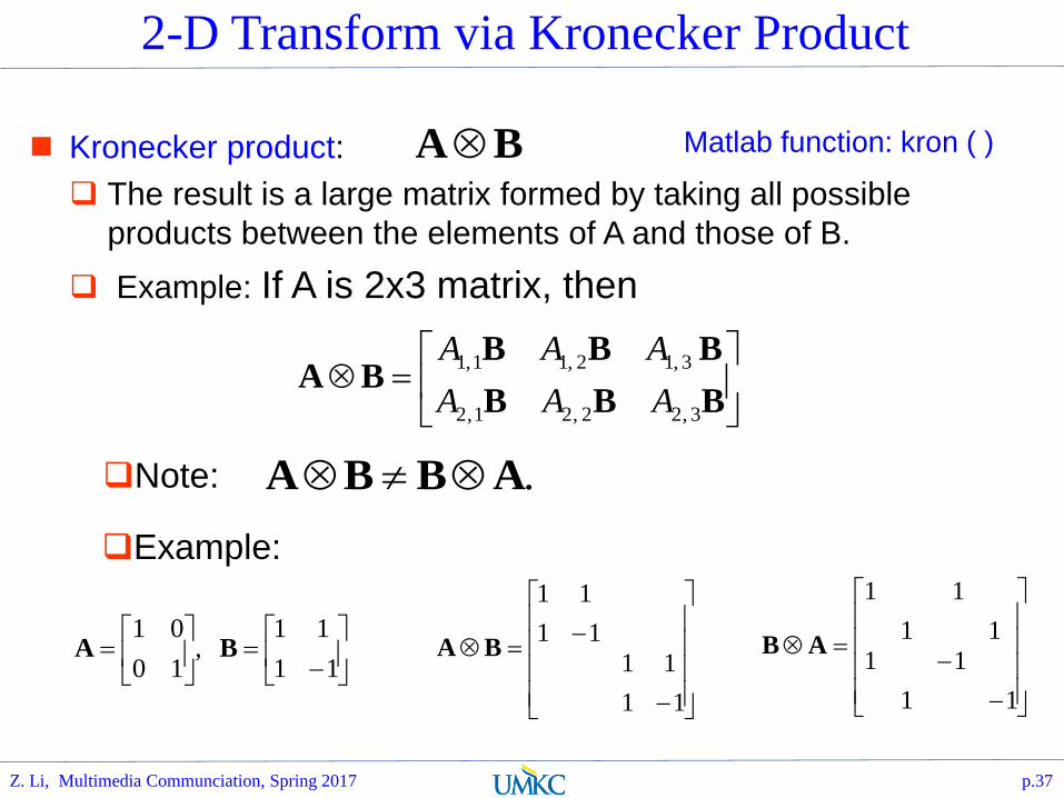
2-D Transform via Kronecker Product
Kronecker product:
The result is a large matrix formed by taking all possible
products between the elements of A and those of B.
Example: If A is 2x3 matrix, then
BA Matlab function: kron ( )
BBB
BBBBA
3 ,22 ,21 ,2
3 ,12 ,11 ,1
AAA
AAA
Note: .ABBA
Example:
11
11 ,
10
01BA
11
11
11
11
BA
1
1
1
1
1
1
1
1
AB
Z. Li, Multimedia Communciation, Spring 2017 p.37

2-D Transform via Kronecker Product
Y. of colth -i :iy
TTT
N
1yyy
TTT
N
1xxx
Def:
2-D separable transform can be implemented as 1-D transform via Kronecker product:
then TTXTY xTTy
X. of colth -i :ix
Filtering complexity instead of O(n2), now O(n).DCT, SIFT DoG
Z. Li, Multimedia Communciation, Spring 2017 p.38
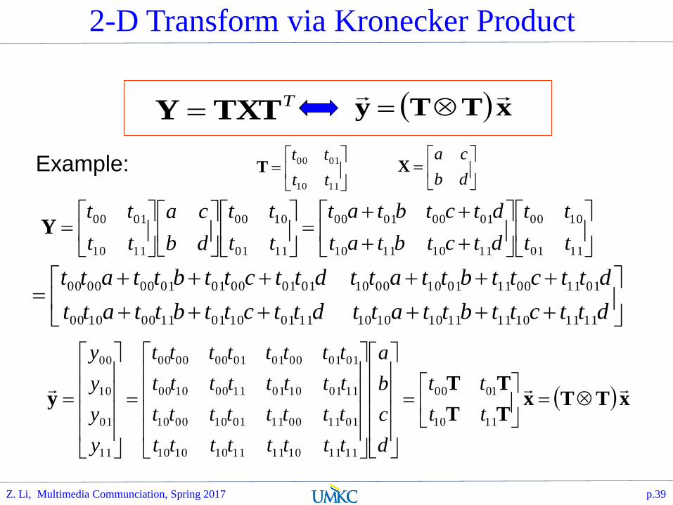
2-D Transform via Kronecker Product
TTXTY xTTy
1110
0100
tt
ttT
db
caX
1101
1000
11101110
01000100
1101
1000
1110
0100
tt
tt
dtctbtat
dtctbtat
tt
tt
db
ca
tt
ttY
dttcttbttattdttcttbttatt
dttcttbttattdttcttbttatt
11111011111010011101100111001000
01110011011000010101000101000000
xTTxTT
TTy
1101
1000
1111101111101001
0111001101100001
1101100111001000
0101000101000000
11
01
10
00
tt
tt
d
c
b
a
tttttttt
tttttttt
tttttttt
tttttttt
y
y
y
y
Example:
Z. Li, Multimedia Communciation, Spring 2017 p.39

Discrete Cosine Transform (DCT)
DCT is the approximation of the KLT of AR(1) signal when its correlation coefficient ρ is close to 1 (e.g. 0.95)
1.-N ..., 1,ifor /2
0,ifor /1
1.-N ..., 0,j i, ,2
)12(cos ,
Na
Na
N
ijaji
C
Definition:
Matlab function:
dct(eye(N));
Z. Li, Multimedia Communciation, Spring 2017 p.40
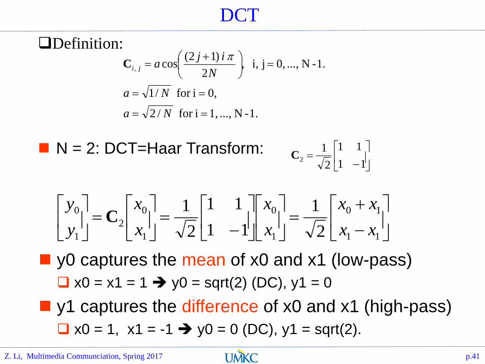
DCT
Definition:
1.-N ..., 1,ifor /2
0,ifor /1
1.-N ..., 0,j i, ,2
)12(cos ,
Na
Na
N
ijaji
C
N = 2: DCT=Haar Transform:
11
11
2
12C
11
10
1
0
1
0
2
1
0
2
1
11
11
2
1
xx
xx
x
x
x
x
y
yC
y0 captures the mean of x0 and x1 (low-pass)
x0 = x1 = 1 y0 = sqrt(2) (DC), y1 = 0
y1 captures the difference of x0 and x1 (high-pass)
x0 = 1, x1 = -1 y0 = 0 (DC), y1 = sqrt(2).
Z. Li, Multimedia Communciation, Spring 2017 p.41
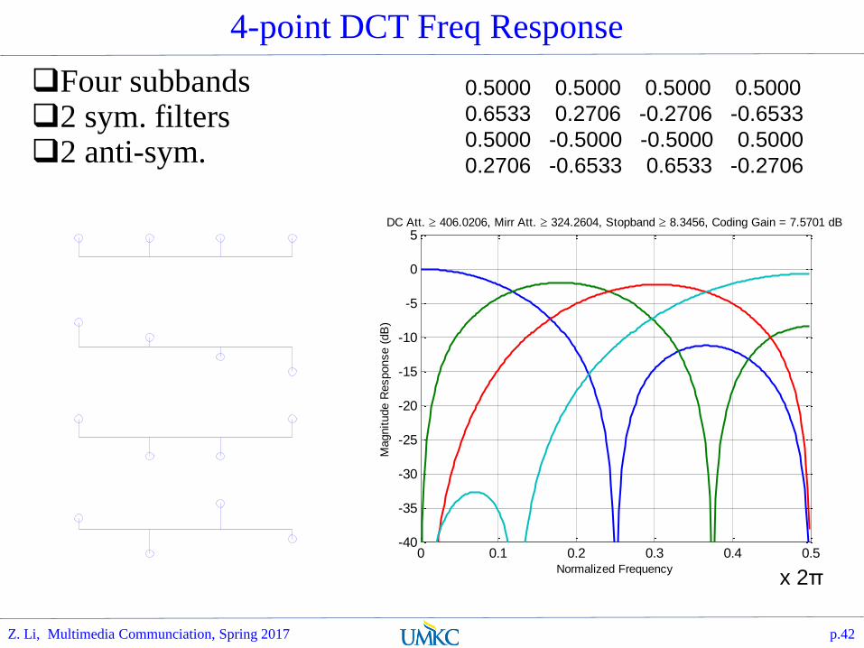
4-point DCT Freq Response
Four subbands2 sym. filters2 anti-sym.
0.5000 0.5000 0.5000 0.5000
0.6533 0.2706 -0.2706 -0.6533
0.5000 -0.5000 -0.5000 0.5000
0.2706 -0.6533 0.6533 -0.2706
0 0.1 0.2 0.3 0.4 0.5-40
-35
-30
-25
-20
-15
-10
-5
0
5DC Att. 406.0206, Mirr Att. 324.2604, Stopband 8.3456, Coding Gain = 7.5701 dB
Normalized Frequency
Magnitude R
esponse (
dB
)
x 2π
Z. Li, Multimedia Communciation, Spring 2017 p.42

8-point DCT
Eight subbands:4 sym., 4 anti-sym.
x 2π
0 0.1 0.2 0.3 0.4 0.5-40
-35
-30
-25
-20
-15
-10
-5
0
5DC Att. 409.0309, Mirr Att. 320.1639, Stopband 9.9559, Coding Gain = 8.8259 dB
Normalized Frequency
Magnitude R
esponse (
dB
)
Z. Li, Multimedia Communciation, Spring 2017 p.43

Example: 1-D DCT
x = [100 110 120 130 140 150 160 170]T;
8-point DCT:
[381.8377, -64.4232, 0.0, -6.7345, 0.0, -2.0090, 0.0, -0.5070]
Most energy are in the first 2 coefficients.
1 2 3 4 5 6 7 850
100
150
200
250
1 2 3 4 5 6 7 8-100
0
100
200
300
400
x(t)
dct_x(t)
Z. Li, Multimedia Communciation, Spring 2017 p.44

2-D 8-point DCT Example
89 78 76 75 70 82 81 82
122 95 86 80 80 76 74 81
184 153 126 106 85 76 71 75
221 205 180 146 97 71 68 67
225 222 217 194 144 95 78 82
228 225 227 220 193 146 110 108
223 224 225 224 220 197 156 120
217 219 219 224 230 220 197 151
Original Data:
2-D DCT Coefficients (after rounding to integers):
1155 259 -23 6 11 7 3 0
-377 -50 85 -10 10 4 7 -3
-4 -158 -24 42 -15 1 0 1
-2 3 -34 -19 9 -5 4 -1
1 9 6 -15 -10 6 -5 -1
3 13 3 6 -9 2 0 -3
8 -2 4 -1 3 -1 0 -2
2 0 -3 2 -2 0 0 -1Most energy is in the upper-
left corner
Z. Li, Multimedia Communciation, Spring 2017 p.45

Matlab Exercise: SVD, PCA, and DCT approximation
For the lena image, process it as 8x8 blocks
Compute m-coefficients reconstructions
Z. Li, Multimedia Communciation, Spring 2017 p.46

Summary
Adaptive Arithmetic Coding
Binary AC has wide applications
AC can easily adapt to the changing prob of symbols
CABAC: Context Aware Binary AC is widely used in HEVC/AVC (one project: deep dive and review of CABAC in HEVC)
Transforms
KL Transform/PCA: de-correlation and energy preserving formulations
SVD: dealing with n x m tensorial data approximation
DCT: separable transform, much faster, good de-correlation and energy preserving property
Z. Li, Multimedia Communciation, Spring 2017 p.47


