CSE 245: Computer Aided Circuit Simulation and Verification
Instructor:
Prof. Chung-Kuan Cheng
Winter 2003
Lecture 2:
Closed Form Solutions (Linear System)
Feb. 22 2003 Cheng & Peng @ UCSDLecture2.2
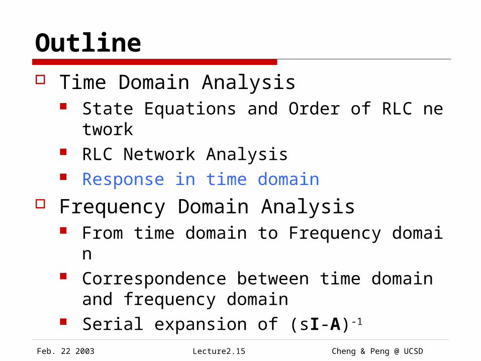
Outline Time Domain Analysis
State Equations and Order of RLC network RLC Network Analysis Response in time domain
Frequency Domain Analysis From time domain to Frequency domain Correspondence between time domain and f
requency domain Serial expansion of (sI-A)-1

Feb. 22 2003 Cheng & Peng @ UCSDLecture2.3
State of a system The state of a system is a set of data, the value of
which at any time t, together with the input to the system at time t, determine uniquely the value of any network variable at time t.
We can express the state in vector form
x =
Where xi(t) is the state variables of the system
)(
.
.
.
)(
)(
2
1
tx
tx
tx
k
Feb. 22 2003 Cheng & Peng @ UCSDLecture2.4
State Variable How to Choose State Variable?
The knowledge of the instantaneous values of all branch currents and voltages determines this instantaneous state
But NOT ALL these values are required in order to determine the instantaneous state, some can be derived from others.
choose capacitor voltages and inductor currents as the state variables! But not all of them are chose
Feb. 22 2003 Cheng & Peng @ UCSDLecture2.5
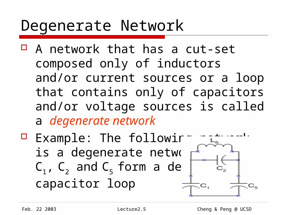
Degenerate Network A network that has a cut-set composed only of
inductors and/or current sources or a loop that contains only of capacitors and/or voltage sources is called a degenerate network
Example: The following network is a degenerate network since C1, C2 and C5 form a
degenerate capacitor loop
Feb. 22 2003 Cheng & Peng @ UCSDLecture2.6
Degenerate Network In a degenerated network, not all the capacitors
and inductors can be chose as state variables since there are some redundancy
On the other hand, we choose all the capacitor voltages and inductors currents as state variable in a nondegenerate network
We will give an example of how to choose state variable in the following section
Feb. 22 2003 Cheng & Peng @ UCSDLecture2.7
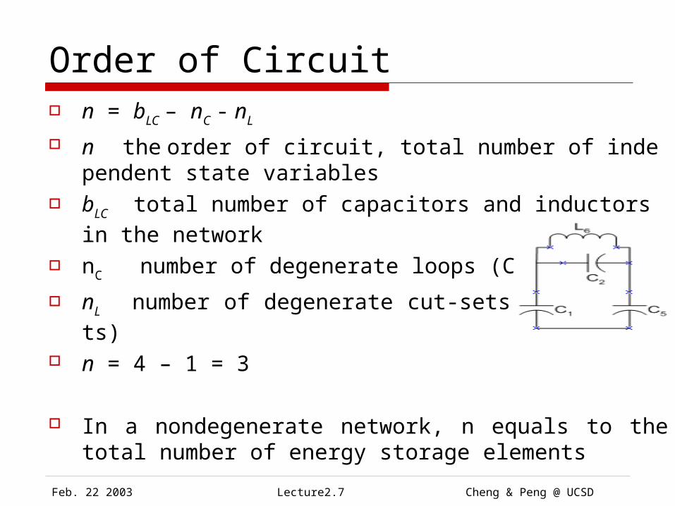
Order of Circuit n = bLC – nC - nL n the order of circuit, total number of independent state variab
les bLC total number of capacitors and inductors in the network
nC number of degenerate loops (C-E loops)
nL number of degenerate cut-sets (L-J cut-sets)
n = 4 – 1 = 3
In a nondegenerate network, n equals to the total number of energy storage elements
Feb. 22 2003 Cheng & Peng @ UCSDLecture2.8
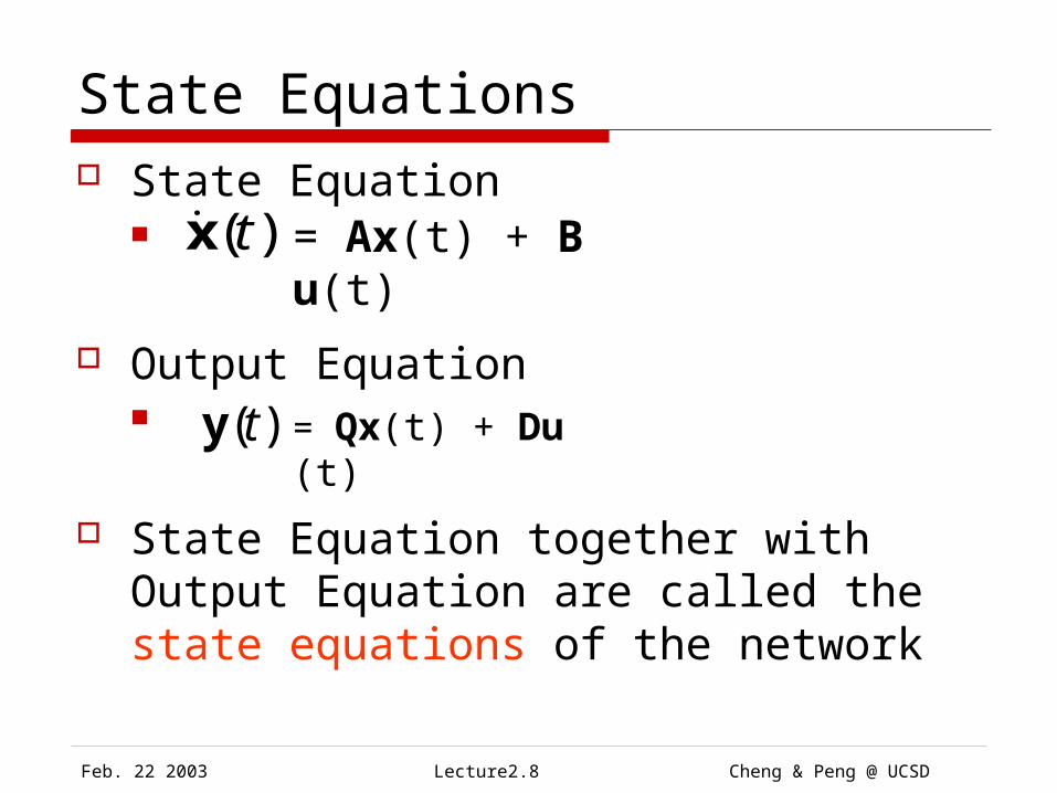
State Equations State Equation
Output Equation
State Equation together with Output Equation are called the state equations of the network
)(ty = Qx(t) + Du(t)
)(tx = Ax(t) + Bu(t)

Feb. 22 2003 Cheng & Peng @ UCSDLecture2.9
Outline Time Domain Analysis
State Equations and Order of RLC network RLC Network Analysis Response in time domain
Frequency Domain Analysis From time domain to Frequency domain Correspondence between time domain and f
requency domain Serial expansion of (sI-A)-1

Feb. 22 2003 Cheng & Peng @ UCSDLecture2.10
RLC Network Analysis A given RLC network
Degenerate Network, Choose only voltages of C1 and C5, current of L6 as our state variable
Vs
g3
g4C1
C2
C5
L6
1 2
0
Feb. 22 2003 Cheng & Peng @ UCSDLecture2.11
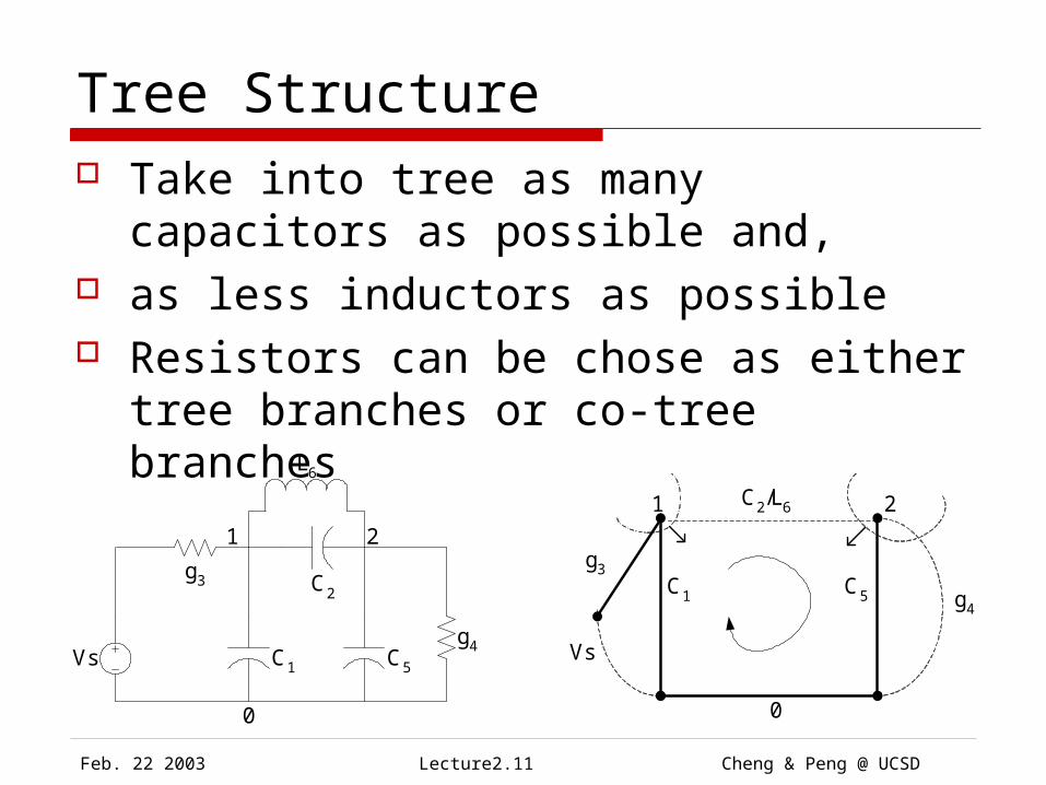
Tree Structure Take into tree as many capacitors as
possible and, as less inductors as possible Resistors can be chose as either tree
branches or co-tree branches
Vs
g3
g4C1
C2
C5
L6
1 2
0
g3C1 C5 g4
1 2C2/L6
0
Vs
Feb. 22 2003 Cheng & Peng @ UCSDLecture2.12
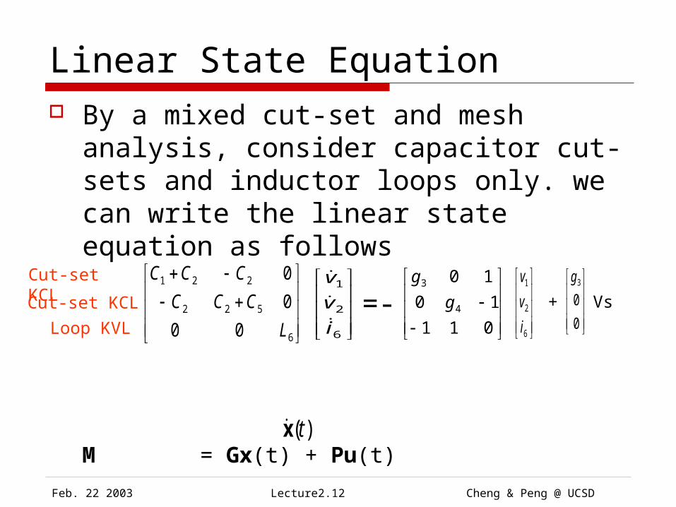
Linear State Equation By a mixed cut-set and mesh
analysis, consider capacitor cut-sets and inductor loops only. we can write the linear state equation as follows
M = Gx(t) + Pu(t))(tx
Cut-set KCL
Loop KVL
Cut-set KCL
6
522
221
00
0
0
L
CCC
CCC
6
2
1
i
v
v
011
10
10
4
3
g
g
6
2
1
i
v
v
0
03g
=- + Vs
Feb. 22 2003 Cheng & Peng @ UCSDLecture2.13
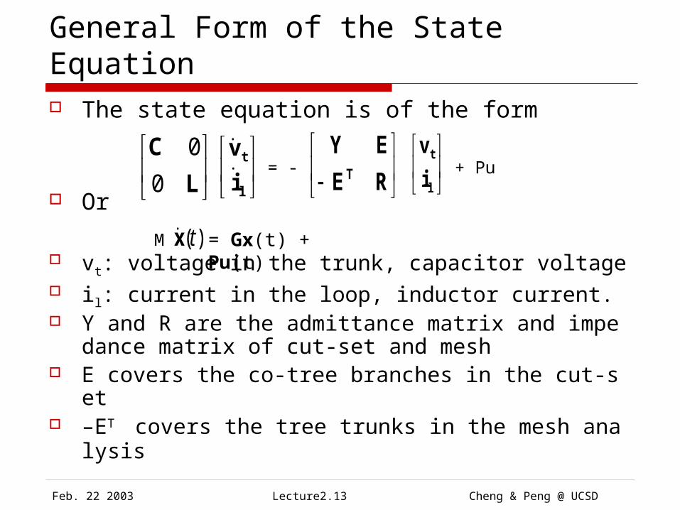
General Form of the State Equation The state equation is of the form
Or
vt: voltage in the trunk, capacitor voltage il: current in the loop, inductor current. Y and R are the admittance matrix and impedance
matrix of cut-set and mesh E covers the co-tree branches in the cut-set –ET covers the tree trunks in the mesh analysis
L
C
0
0
l
t
i
v
RE
EYT
l
t
i
v= - + Pu
= Gx(t) + Pu(t)
)(txM
Feb. 22 2003 Cheng & Peng @ UCSDLecture2.14
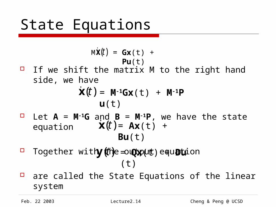
State Equations
If we shift the matrix M to the right hand side, we have
Let A = M-1G and B = M-1P, we have the state equation
Together with the output equation
are called the State Equations of the linear system
= Gx(t) + Pu(t)
)(txM
)(tx = M-1Gx(t) + M-1Pu(t)
= Ax(t) + Bu(t)
)(tx
)(ty = Qx(t) + Du(t)
Feb. 22 2003 Cheng & Peng @ UCSDLecture2.15
Outline Time Domain Analysis
State Equations and Order of RLC network RLC Network Analysis Response in time domain
Frequency Domain Analysis From time domain to Frequency domain Correspondence between time domain and f
requency domain Serial expansion of (sI-A)-1

Feb. 22 2003 Cheng & Peng @ UCSDLecture2.16
Response in time domain We can solve the state equation and get the clos
ed form expression
The output equation can be expressed as
Note: * denotes convolution
Feb. 22 2003 Cheng & Peng @ UCSDLecture2.17
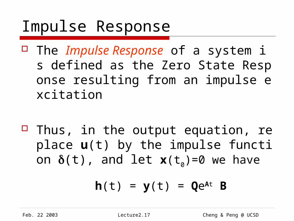
Impulse Response The Impulse Response of a system is defined as
the Zero State Response resulting from an impulse excitation
Thus, in the output equation, replace u(t) by the impulse function (t), and let x(t0)=0 we have
h(t) = y(t) = QeAt B
Feb. 22 2003 Cheng & Peng @ UCSDLecture2.18
Outline Time Domain Analysis
State Equations and Order of RLC network RLC Network Analysis Response in time domain
Frequency Domain Analysis From time domain to Frequency domain Correspondence between time domain and f
requency domain Serial expansion of (sI-A)-1
Feb. 22 2003 Cheng & Peng @ UCSDLecture2.19
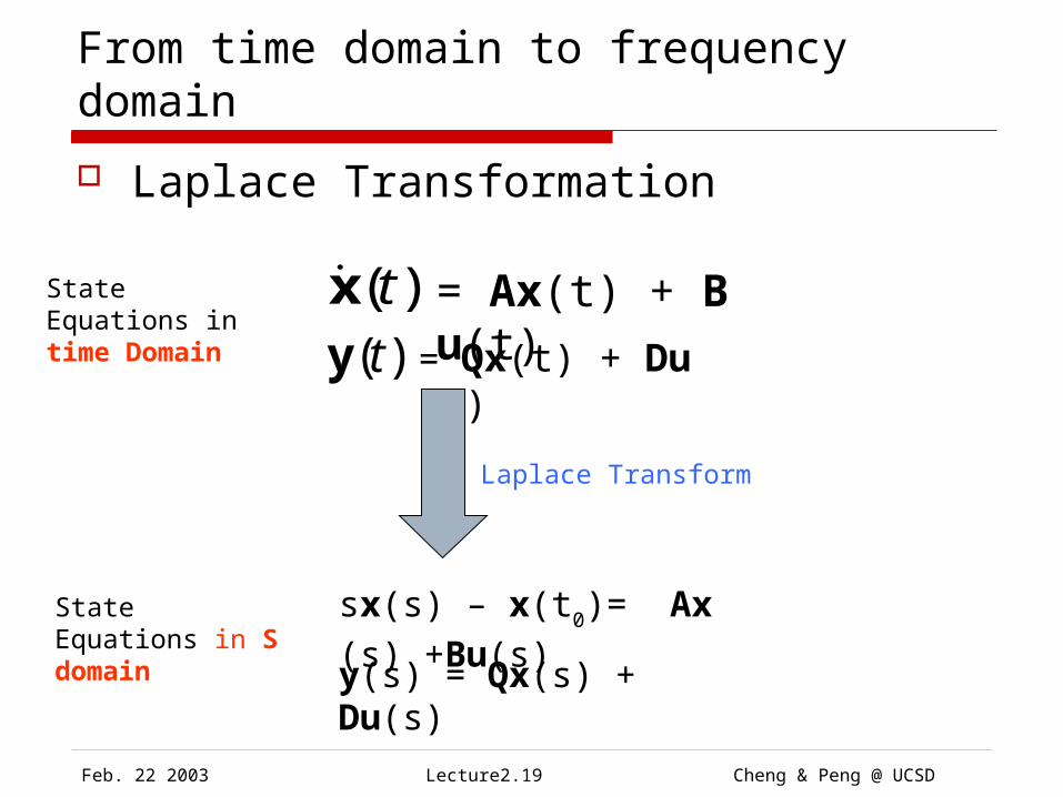
From time domain to frequency domain
Laplace Transformation
)(tx = Ax(t) + Bu(t)
)(ty = Qx(t) + Du(t)
Laplace Transform
sx(s) – x(t0)= Ax(s) +Bu
(s) y(s) = Qx(s) +Du(s)
State Equations in S domain
State Equations in time Domain
Feb. 22 2003 Cheng & Peng @ UCSDLecture2.20
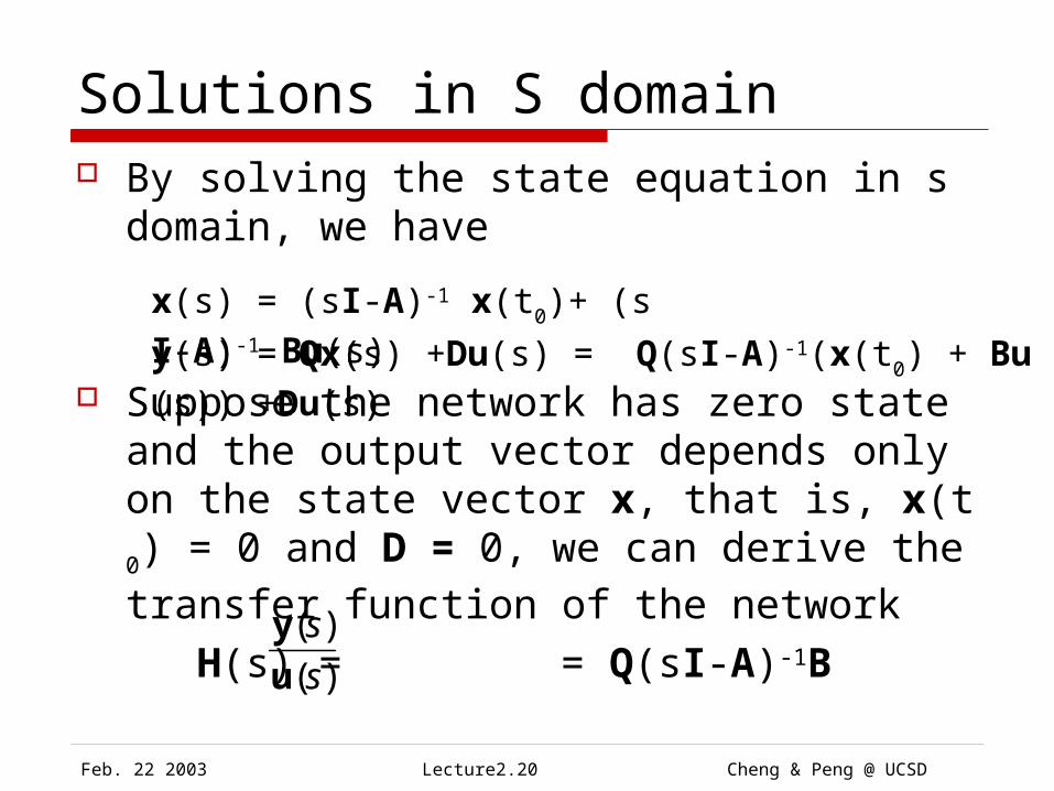
Solutions in S domain By solving the state equation in s
domain, we have
Suppose the network has zero state and the output vector depends only on the state vector x, that is, x(t0) = 0 and D = 0, we can derive the trans
fer function of the network
H(s) = = Q(sI-A)-1B
x(s) = (sI-A)-1 x(t0)+ (sI-A)-1 Bu(s)
y(s) = Qx(s) +Du(s) = Q(sI-A)-1(x(t0) + Bu(s)) +Du(s)
)(
)(
s
s
u
y
Feb. 22 2003 Cheng & Peng @ UCSDLecture2.21
Outline Time Domain Analysis
State Equations and Order of RLC network RLC Network Analysis Response in time domain
Frequency Domain Analysis From time domain to Frequency domain Correspondence between time domain and f
requency domain Serial expansion of (sI-A)-1

Feb. 22 2003 Cheng & Peng @ UCSDLecture2.22
Correspondence between time domain and frequency domain We can derive the time domain solutions of the net
work from the s domain solutions by inverse Laplace Transformation of the s domain solutions.
State Equations in S domain
State Equations in time Domain
Inverse Laplace Transform
sx(s) – x(t0)= Ax(s) +Bu
(s) y(s) = Qx(s) +Du(s)
x(t) = L-1[(sI-A)-1x(t0) + (sI-A)-1 Bu(s)]
= L-1[(sI-A)-1]x(t0) + L-1[(sI-A)-1]B*u(t)
y(t) = L-1[Q(sI-A)-1(x(t0) + Bu(s)) +Du(s)]
= Q L-1[(sI-A)-1] x(t0) + {QL-1 [(sI-A)-1]B +D(t)}* u(s)
Feb. 22 2003 Cheng & Peng @ UCSDLecture2.23
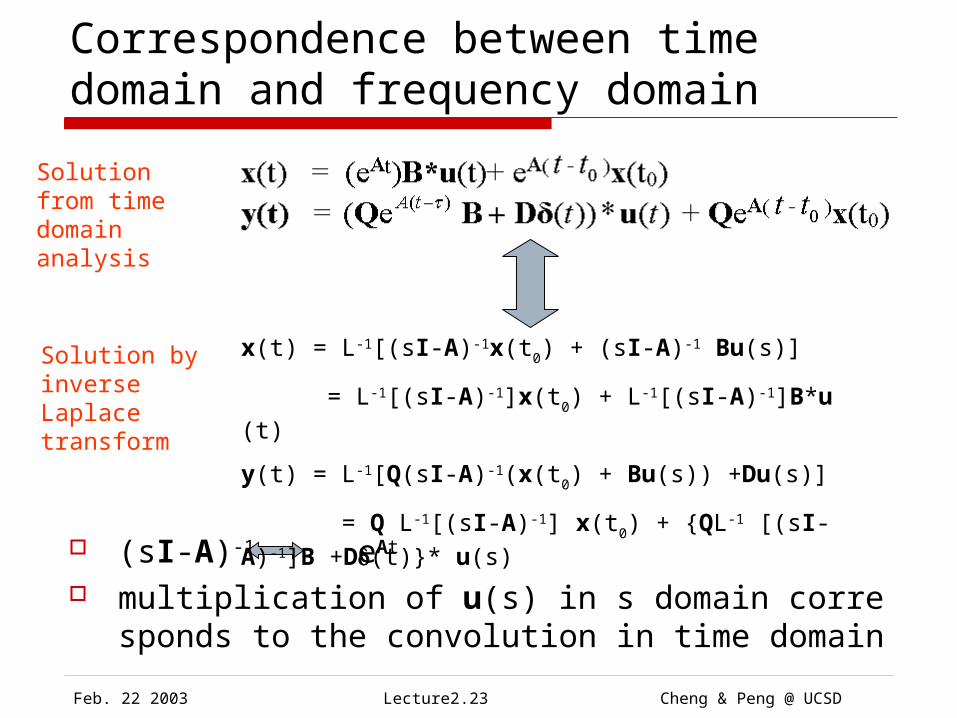
Correspondence between time domain and frequency domain
(sI-A)-1 eAt multiplication of u(s) in s domain corresponds to th
e convolution in time domain
Solution from time domain analysis
Solution by inverse Laplace transform
x(t) = L-1[(sI-A)-1x(t0) + (sI-A)-1 Bu(s)]
= L-1[(sI-A)-1]x(t0) + L-1[(sI-A)-1]B*u(t)
y(t) = L-1[Q(sI-A)-1(x(t0) + Bu(s)) +Du(s)]
= Q L-1[(sI-A)-1] x(t0) + {QL-1 [(sI-A)-1]B +D(t)}* u(s)
Feb. 22 2003 Cheng & Peng @ UCSDLecture2.24
Outline Time Domain Analysis
State Equations and Order of RLC network RLC Network Analysis Response in time domain
Frequency Domain Analysis From time domain to Frequency domain Correspondence between time domain and f
requency domain Serial expansion of (sI-A)-1

Feb. 22 2003 Cheng & Peng @ UCSDLecture2.25
Serial expansion of (sI-A)-1
When s0 we can write (sI-A)-1 as
Thus, the transfer function can be wrote as
When s we can write (sI-A)-1 as
The transfer function can be wrote as
(sI-A)-1 = -A-1(I – SA-1) = -A-1(I + SA-1 + S2A-2 + … + SkA-k + …)
H(s) = Q(sI-A)-1B = -QA-1(I + SA-1 + S2A-2 + … + SkA-k + …)B
(sI-A)-1 = S-1(I – S-1A)-1 = S-1(I + S-1A + S-2A2 + … + S-kAk + …)
H(s) = Q(sI-A)-1B = S-1(I + S-1A + S-2A2 + … + S-kAk + …)B

Feb. 22 2003 Cheng & Peng @ UCSDLecture2.26
Assume A has non-degenerate eigenvalues
and corresponding linearly independent eigenvectors , then A can be decomposed as
where and
Matrix Decomposition
1A
k ,...,, 21
k ,...,, 21
k
0
0
00
2
1
k ,...,, 21

Feb. 22 2003 Cheng & Peng @ UCSDLecture2.27
Matrix Decomposition Then we can write (sI-A)-1 in the following form
(sI-A)-1 in s domain corresponds to the exponential function eAt in time domain, we can write
eAt as
(sI-A)-1 = (SI – X-1X)‑1 = X-1(SI – )-1X = X-1
ns
s
s
1.
.2
1
1
1
X
eAt = X-1
t
t
t
ne
e
e
.
.
2
1
X


