
Corporate Hedging, Investment and Value∗
Jose M. Berrospide† Amiyatosh Purnanandam‡ Uday Rajan§
March 27, 2011
∗We thank Tim Adam, Heitor Almeida, Sudheer Chava, Kathryn Dominguez, Jie Gan, Han Kim, Peter Mackay,Per Ostberg, Paige Parker, Amit Seru, Rene Stulz, Linda Tesar, Jing Zhang, and seminar participants at CSSS(Calcutta), Hong Kong UST, London Business School, Michigan, National University of Singapore, Notre Dame,Singapore Management University, and the EFA, FIRS, and WFA Meetings for helpful comments. All errors remainour own. The views expressed are those of the authors and do not necessarily reflect those of the Board of Governorsof the Federal Reserve System or its staff.†Federal Reserve Board; Tel: (202) 452-3590, E-mail: [email protected]‡Ross School of Business, University of Michigan; Tel: (734) 764-6886, E-mail: [email protected]§Ross School of Business, University of Michigan; Tel: (734) 764-2310, E-mail: [email protected]

Corporate Hedging, Investment, and Value
Abstract
Following a severe currency crisis in 1998, the Brazilian economy switched from a fixed toa floating exchange rate regime in 1999. Brazilian firms that had accumulated foreign currencyliabilities in the fixed exchange rate regime suddenly found themselves exposed to significantcurrency risk. The temporary disequilibrium created by this shock allows us to trace the causaleffect of currency hedging on corporate performance and firm value. We find that hedgingallows a firm to insulate its capital expenditure from variation in operating cash flow. That is,it mitigates the underinvestment friction of Froot, Scharfstein and Stein (1993). Hedging alsoincreases the foreign debt capacity of a firm at a time when domestic capital is scarce, allowingthe firm to increase the level of investment. Both these channels lead to an improvement in thevalue of the firm.
JEL Codes: G30, G32.
Keywords: Currency Derivatives, Hedging, Firm Value, Underinvestment, Debt Capacity.

1 Introduction
It is well-understood that corporate financial policy cannot increase the value of a firm in a
frictionless world. In the presence of market imperfections, financial policy can be value-enhancing
if it mitigates the effects of frictions such as informational problems or agency costs. Understanding
the links between a firm’s financial policy, the frictions that it overcomes, and the resulting value
effect is central to corporate finance research. Despite the importance of this issue, it has remained
an extremely difficult task to empirically establish these links in a world in which all firms are
making optimal decisions. In such a world, each firm chooses its financial policy based on the
net benefits of different actions that, in turn, depend on several firm characteristics. Since many
of these characteristics remain unobserved to the econometrician, it is not easy to determine the
correct counterfactual, i.e., what would a firm’s value be under an alternative financial policy?
In this paper we study the effect of a specific financial policy, i.e., hedging foreign currency
risk, on corporate performance and value. While there have been several worthy studies relating
corporate hedging to firm value, the causal effect remains contentious due to the reasons mentioned
above. If firms are heterogeneous along unobservable dimensions, any effect of hedging on firm
value in equilibrium faces the challenge of isolating the effect of these unobservable factors from
the effect of hedging. In an industry with identical firms, as Adam, Dasgupta and Titman (2007)
demonstrate, in equilibrium each firm should be indifferent between hedging and not, and hedgers
and non-hedgers should have identical values.
Our innovation is to study an emerging economy, Brazil, at a time when it switched from a
fixed to a floating exchange rate regime. Following a severe currency crisis, in January 1999, Brazil
abandoned its currency peg and adopted a floating exchange rate policy. The Brazilian currency,
the real, depreciated by about 66% in two weeks following the switch, and remained volatile for
many years thereafter. Several Brazilian firms had foreign currency denominated liabilities before
the regime switch. These firms were now suddenly exposed to exchange rate risk. Further, due to
the broader economic turmoil, capital in the domestic economy was scarce at this time. Given the
scale of the upheaval in the economy, it is natural that it would take firms some time to learn their
1

optimal policies in the new regime.
Indeed, we find that while many firms in our sample start to use foreign currency derivatives, the
change from being unhedged to hedging is not instantaneous. Rather, there is a gradual increase in
the number of firms that hedge after the regime switch. The proportion of firms that use currency
derivatives increases from a modest level of 14% at the end of 1999 to about 40% by the end
of 2001, and remains stable thereafter. This pattern is consistent with firms gradually learning
and adjusting to their new optimal policy in the floating exchange rate regime. We analyze the
determinants of the time-to-switch for firms that begin to use currency derivatives, and find that
firms with a higher benefit or lower cost to hedging do so more quickly. In particular, the size of a
firm and the extent of its foreign debt as of 1998, the last year of fixed exchange rates, are critical
in determining the likelihood that a firm will begin to hedge sooner.
The staggered change from a state of no hedging to hedging across the hedger firms in the
economy offers an attractive empirical setting to assess the causal effect of hedging on firm
performance and value. Immediately after the shock, there are two groups of non-hedgers: (a)
firms for whom it is optimal to remain unhedged in the new exchange rate regime and (b) firms for
whom it would be optimal to hedge. Many firms in the latter group find themselves temporarily
adopting a sub-optimal policy as they adjust to the new regime. In this interim period, these firms
are learning about the costs and benefits of hedging, setting up a hedging program, and searching for
the supply of derivative products from financial intermediaries. Thus, by comparing the outcomes
for such a firm after it begins to use derivatives with its own corresponding performance during
the interim sub-optimal period, we are able to trace the effect of hedging on firm performance and
value.
Motivated by the theoretical model of Froot, Scharfstein and Stein (FSS, 1993), we first examine
the effect of hedging on capital expenditure plans. Using a firm fixed effect specification, we show
that a firm that starts using currency derivatives increases its capital expenditures. To directly
investigate the predictions of FSS, we estimate the investment-to-cash flow sensitivity of our sample
firms across hedgers and non-hedgers. The investment of non-hedgers is highly sensitive to their
cash flows, while hedger firms have investment that is insensitive to operating cash flow. In other
2

words, hedging allows firms to undertake investment even when their internal cash flow is low.
These findings are in line with the FSS model and provide direct evidence on the role of hedging
in mitigating financial frictions. Since the decision to hedge is a choice variable, it is important
to show that our results are not driven by a precise simultaneous change in the firm’s investment
opportunity set or managerial characteristics. To address this issue, we show that our results are
not explained away by changes in time varying industry-specific investment opportunity sets or
changes in the management at hedger firms.
We next show that the increase in capital expenditure is partly financed by a contemporaneous
increase in the foreign currency debt of the firm. Thus, as predicted by Leland (1998), hedging
increases the debt capacity of a firm in our sample. In our context, hedging not only increases the
pledgeable income of a firm, but it allows the firm to overcome a supply-side friction in the capital
market. In the floating exchange rate regime, the spread between deposit rates and interest rates
on domestic loans is very high, and the banking sector is in turmoil.1 Currency hedging allows
firms to access a source of capital that remains available at a reasonable cost.2 The additional
capital is then invested at a time when the marginal value of investment is high, in part because
many other firms in the economy cannot invest.
After establishing the role of hedging in smoothing investment and increasing debt capacity, we
investigate its effect on a firm’s value. Comparing the value of a firm before and after it begins to
hedge, we find that derivative usage results in a value gain of about 10%. The magnitude of the
effect is large compared to that found by studies based on U.S. firms (for example, see Allayannis
and Weston (2002)). It is important to note that our estimates come from a period of massive
upheaval in the Brazilian economy. The possibility of under-investment due to the lack of external
capital is likely to be very high during these periods. An increase in investment with the promise
of smooth future investment is akin to an improvement in the growth rate of the hedgers, which
can result in substantial improvement in firm value. Our evidence supports this view.
Our study relates to a large literature on hedging and firm value. Allayannis and Weston (2002)1See Sobrinho (2007) for example.2Berrospide (2010) extends the Holmstrom and Tirole (1997) model of external financing to an open economy,
and demonstrates theoretically that hedging can increase foreign debt capacity.
3

examine the effect of currency derivatives on U.S. firms, and find a value premium of 4.87%. Guay
and Kothari (2003) provide a critique of this result in which they uncover the actual derivative
positions of firms in their sample, and show that the size of the positions is too small to justify such
a large value premium. Indeed, they find that a simultaneous three-standard deviation adverse
movement in interest rates, exchange rates, and commodity prices will only have a value effect of
1.3% on the typical hedged firm. Jin and Jorion (2006) do not find evidence in support of positive
valuation effect of hedging in a sample of U.S. oil and gas producers.
Work on the mechanism through which hedging can influence firm value includes Graham and
Rogers (2002), who show that hedging does increase the debt capacity of a firm, and that the
increased interest tax shields add about 1.1% to firm value. Campello, et al. (2010) consider a
sample of US firms and use an instrumental variables approach to show that hedging leads to lower
spreads on syndicated loans and reduces the chances of covenants that restricts investments. While
our study also considers the effect of hedging on investments, we focus on access to capital and the
smoothing of investment across different cash flow states.
Our paper also contributes to the literature on the effect of supply shocks to banks on the
performance of their borrowers (for example, see Khwaja and Mian (2008), Paravisini (2008),
and Chava and Purnanandam (2011)). This literature shows that borrowing firms face significant
adverse consequences when their lenders face adverse capital or liquidity shocks. Our study shows
that hedging allows firms to substitute between domestic and international sources of capital, which
in turn can insulate a firm’s performance from the financial health of its domestic lenders. Thus, at
a broader level, we contribute to the literature on financial constraints and show that firms in an
emerging market face significant frictions in raising external capital. Access to currency derivatives
can help alleviate these frictions.
The rest of the paper is organized as follows. We discuss our theoretical and empirical framework
in Section 2. In this section, we first provide some background information on the Brazilian economy
and the currency crisis. We then discuss the theoretical motivation behind our tests and the
identification strategy. Section 3 briefly describes our sample and data sources. In this section, we
also discuss the determinants of hedging policy. Our empirical results are contained in Section 4, in
4
which we demonstrate the effect of derivative usage on capital expenditure, foreign currency debt,
and value. Section 5 concludes the paper.
2 Theoretical and Empirical Framework
Our main theoretical motivation comes from the work by Froot, Scharfstein and Stein (1993;
henceforth FSS) and Leland (1998). FSS argue that hedging is valuable when external financing
is costly because it allows the firm to maintain its investment in states with low cash flow. Leland
(1998) shows that hedging increases the debt capacity of a firm. We argue that foreign currency
hedging by some firms in our sample increases the foreign debt capacity of these firms, at a time
when capital in the domestic economy was scarce. The access to foreign capital then allows these
firms to maintain a smooth investment policy, thereby increasing value.
On the empirical side, we argue that the scale of disruption in the Brazilian economy was
sufficiently large that firms would take some time to determine their optimal policies in the new
regime. As a result, for some time after the switch from fixed to floating exchange rates, some firms
would have had sub-optimal hedging policies. By comparing outcomes for the same firm before
and after it starts hedging, we can therefore obtain an estimate of the effect of hedging on firm
performance and value.
Both our theoretical and empirical arguments rely on the Brazilian economy having suffered a
large shock at the start of the sample period. We therefore begin by describing the macro-economic
environment in Brazil immediately following the switch to a floating exchange rate regime.
2.1 Brazil: Macro-economic Environment
In late 1998 and early 1999, Brazil suffered from a financial crisis that led to its currency, the real,
being fully floated on January 15, 1999. The real (denoted as R$; plural reais) was introduced in
July 1994, as part of a stabilization package known as the Real Plan (see Averbug, 2002). As part of
the plan, important regulatory changes were introduced in the financial markets to reduce controls
on capital flows and improve the access of corporations to foreign currency debt from international
5
capital markets. A crawling peg exchange rate regime was adopted for the real, with preannounced
narrow bands within which the exchange rate was maintained. In this paper, we refer to the period
before January 1999 as the “fixed” exchange rate regime.
The years leading up to 1999 saw financial crises affect Mexico (1994), East Asia (1997), and
Russia (1998). The Brazilian economy was severely affected by the Russian crisis of August, 1998,
and suffered substantial capital outflows. External aid from the IMF and the G-7 provided a
breather, but capital outflows increased again in January, 1999, leading to the fixed exchange rate
regime being abandoned in favor of a floating regime. There were continued shocks to the economy
in the floating exchange rate period, with the Argentinian crisis of 2001-02 having a ripple effect
throughout Latin America, and a presidential election in 2002 contributing to political uncertainty.
2.1.1 Exchange rate, GDP growth, and inflation
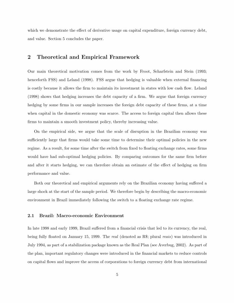
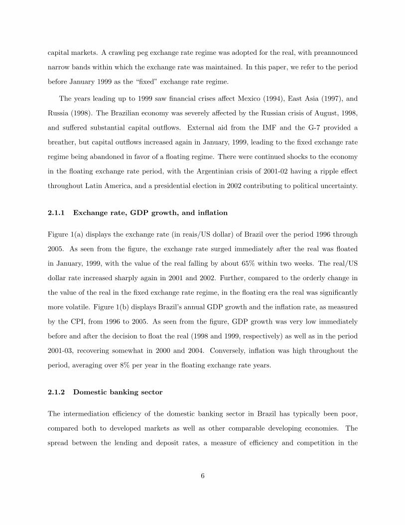
Figure 1(a) displays the exchange rate (in reais/US dollar) of Brazil over the period 1996 through
2005. As seen from the figure, the exchange rate surged immediately after the real was floated
in January, 1999, with the value of the real falling by about 65% within two weeks. The real/US
dollar rate increased sharply again in 2001 and 2002. Further, compared to the orderly change in
the value of the real in the fixed exchange rate regime, in the floating era the real was significantly
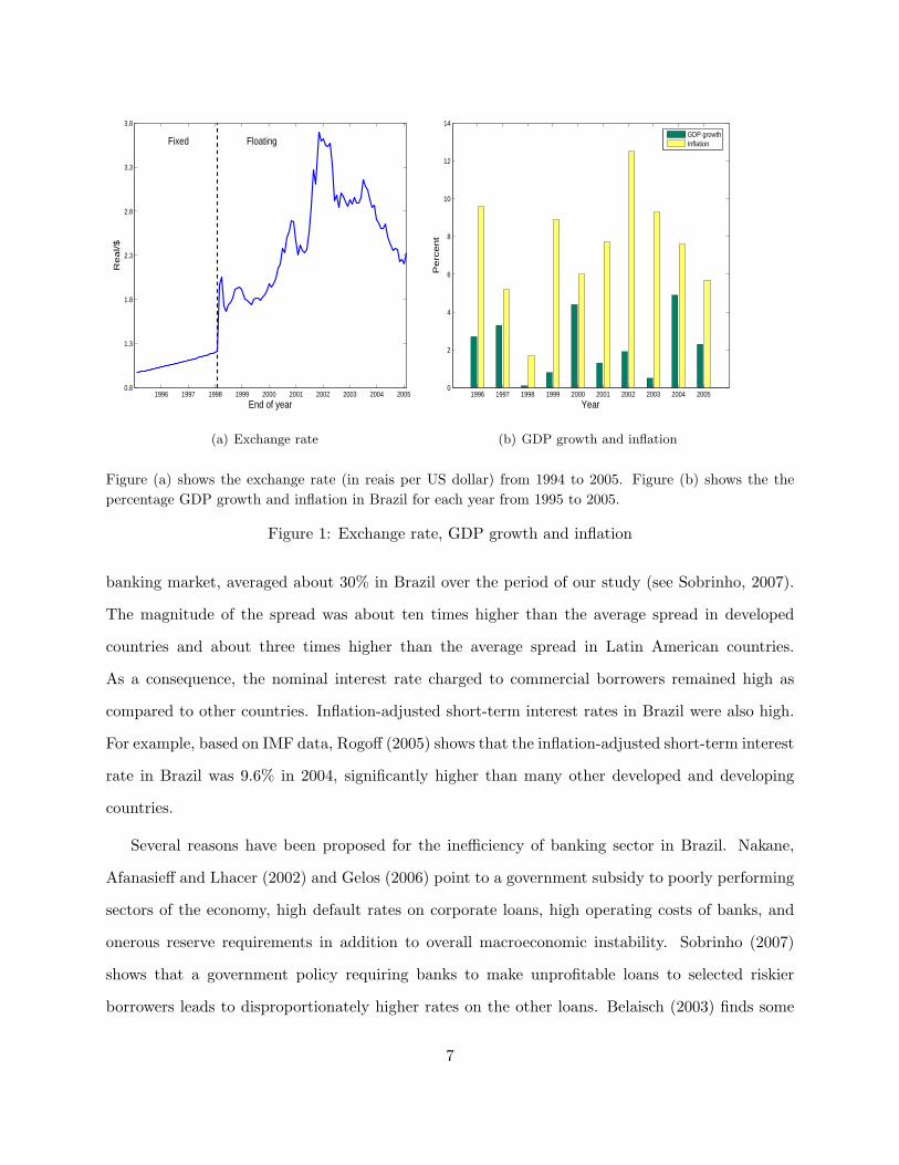
more volatile. Figure 1(b) displays Brazil’s annual GDP growth and the inflation rate, as measured
by the CPI, from 1996 to 2005. As seen from the figure, GDP growth was very low immediately
before and after the decision to float the real (1998 and 1999, respectively) as well as in the period
2001-03, recovering somewhat in 2000 and 2004. Conversely, inflation was high throughout the
period, averaging over 8% per year in the floating exchange rate years.
2.1.2 Domestic banking sector
The intermediation efficiency of the domestic banking sector in Brazil has typically been poor,
compared both to developed markets as well as other comparable developing economies. The
spread between the lending and deposit rates, a measure of efficiency and competition in the
6
1996 1997 1998 1999 2000 2001 2002 2003 2004 20050.8
1.3
1.8
2.3
2.8
3.3
3.8R
eal/$
End of year
Fixed Floating
(a) Exchange rate
1996 1997 1998 1999 2000 2001 2002 2003 2004 20050
2
4
6
8
10
12
14
Year
Perc
ent
GDP growthInflation
(b) GDP growth and inflation
Figure (a) shows the exchange rate (in reais per US dollar) from 1994 to 2005. Figure (b) shows the thepercentage GDP growth and inflation in Brazil for each year from 1995 to 2005.
Figure 1: Exchange rate, GDP growth and inflation
banking market, averaged about 30% in Brazil over the period of our study (see Sobrinho, 2007).
The magnitude of the spread was about ten times higher than the average spread in developed
countries and about three times higher than the average spread in Latin American countries.
As a consequence, the nominal interest rate charged to commercial borrowers remained high as
compared to other countries. Inflation-adjusted short-term interest rates in Brazil were also high.
For example, based on IMF data, Rogoff (2005) shows that the inflation-adjusted short-term interest
rate in Brazil was 9.6% in 2004, significantly higher than many other developed and developing
countries.
Several reasons have been proposed for the inefficiency of banking sector in Brazil. Nakane,
Afanasieff and Lhacer (2002) and Gelos (2006) point to a government subsidy to poorly performing
sectors of the economy, high default rates on corporate loans, high operating costs of banks, and
onerous reserve requirements in addition to overall macroeconomic instability. Sobrinho (2007)
shows that a government policy requiring banks to make unprofitable loans to selected riskier
borrowers leads to disproportionately higher rates on the other loans. Belaisch (2003) finds some
7

evidence of oligopolistic behavior in the Brazilian banking sector. Arida, Bacha, and Lara-Resende
(2005) suggest that high credit spreads for Brazilian firms are a result of a crowding-out effect due
to rising government debt in the aftermath of the currency crisis.
Inefficiencies in the banking sector resulted in limited access to bank credit as well as a high cost
of bank loans. Gelos (2006) shows that on average the bank credit-to-GDP ratio was less than 30%
in Brazil in 2003, compared to about 60% for Chile and the U.S. Figure 2 displays the evolution
of the “Selic,” the Brazilian Central Bank’s overnight lending rate, from the period 1996 through
2005. For much of this period, the Selic hovered around 18-25%, with a few spikes corresponding
to the East Asian (1997) and Russian (1998) currency crises.
1996 1997 1998 1999 2000 2001 2002 2003 2004 20050
5
10
15
20
25
30
35
40
45
50
Selic
rate
(%)
End of year
Fixed Floating
This figure shows the central bank’s domestic overnight borrowing rate, the Selic, from 1996 to 2005.
Figure 2: Domestic interest rate (Selic)
Overall, during the period of our study, the Brazilian economy passed through an extremely
turbulent phase. Exchange rate volatility was very high and the rapid depreciation of the real was
associated with very high capital outflows. In addition, the inefficiencies in the domestic banking
sector made it harder for corporate borrowers to raise external capital from domestic sources.
8

2.2 Theoretical Motivation
Derivatives allow firms to transfer cash flows across states and time. Since such transfers by
themselves cannot add value in a frictionless world, theoretical models of corporate hedging rely
on market frictions to explain the use of derivatives. We consider the specific frictions modeled
by two theoretical papers, Froot, Scharfstein and Stein (1993) and Leland (1998), to motivate our
empirical work. We argue that our empirical setting closely resembles the underlying set-up in
these papers.
FSS develop a theory of hedging under the assumption that external financing is costly for
firms as compared to internally generated funds. The paper argues that firm-level frictions such as
bankruptcy costs or information asymmetries can lead to convex costs of raising outside capital.
With costly external financing, a firm’s investment in low cash-flow states will necessarily be smaller
than its investment in high cash-flow states. If the production function is concave, the marginal
value of an extra dollar of investment is greater in low cash-flow states. Thus, a fairly priced hedge
that allows the firm to transfer cash flows from high cash-flow to low cash-flow states can be value
enhancing. In this model, hedging alleviates the friction in raising external capital. In extreme
cases, when external capital is really scarce, the value of hedging can be especially high. There are
two immediate implications of this model. First, holding fixed the investment opportunity set of a
firm, hedging allows the firm to increase its investment in low cash flow states. Second, a hedged
firm’s investment will be less sensitive to its operating cash flow (i.e., its cash flow before accounting
for the effects of derivative usage) than the investment of an otherwise identical unhedged firm.
Leland (1998) considers a model in which debt creates an interest tax shield and therefore adds
value. The tradeoff is that debt also increases the likelihood of bankruptcy, and bankruptcy has
a deadweight cost. Hedging allows a firm to reduce the deadweight cost of bankruptcy, which
increases the debt capacity of the firm. This in turn increases corporate value due to the additional
interest tax shield.
In our setting, Brazilian firms have two potential sources of external finance: domestic and
foreign. As discussed earlier, domestic external finance is scarce because of the economy-wide
9
frictions. The scale of the disruption in the Brazilian economy in 1998 and 1999 generates a large
negative supply shock in the domestic banking sector and capital markets. As a result, firms wishing
to raise external capital have to approach foreign investors. However, in a floating exchange rate
regime with a high volatility in the exchange rate, foreign currency debt entails high exchange rate
risk. As pointed out by Berrospide (2010), it creates the possibility that a firm may go bankrupt
simply due to an adverse change in the exchange rate. Hedging against a depreciation in the
real reduces the probability of exchange-rate-related bankruptcy, increasing the expected payout
to foreign lenders and hence increasing the pledgeable income of the firm.
Overall, our empirical setting has ingredients from both the FSS and Leland models. As in the
FSS model, firms face large costs in raising external financing. Further, our firms start out in a
low cash flow state, so that benefits to increasing investment are likely to be high. International
sources of capital are available, but the associated volatility in the exchange rate exposes firms
to additional deadweight costs if bankruptcy arises as a result of currency fluctuations. As in the
Leland model, firms can hedge away a source of risk (in our case, exchange rate risk) to increase
their debt capacity (in our case, the capacity to take on foreign currency debt). Motivated by these
papers, our empirical tests are designed to uncover the effect of hedging on capital expenditure,
debt capacity, and consequently on corporate value.
2.3 Identification strategy
To estimate the effect of hedging on a firm’s value or corporate policies such as capital expenditure,
one should compare the outcome variable for a hedged firm with the outcome variable for the same
firm when it remains unhedged. In other words, the ideal counterfactual for a firm that chooses to
hedge is the hypothetical outcome for the same firm had it chosen to remain unhedged. Of course,
if each firm chooses an optimal hedging policy, the counterfactual must remain unobserved. The
unobservability creates an important identification problem in any study that tries to empirically
establish the causal effect of corporate hedging on firm value or corporate policies.
In the absence of an observable counterfactual, a general approach in the literature has been to
10

estimate a regression model of the following form:
yit = α+ βxit + θ hedgingit + εit, (1)
where yit is an outcome for firm i at time t (such as capital expenditure or firm value), xit a set of
firm-specific observables (including, say, size and a proxy for investment opportunities) for firm i at
time t, hedgingit a variable that captures the hedging decision of firm i and time t, and εit an error
term. This model implicitly assumes that, after including the control variables x, an unhedged firm
i′ serves as the correct counterfactual for a hedged firm i.
As stated above, if each firm adopts an optimal hedging policy, this method is problematic.
Self-selection implies that each firm, hedged or unhedged, maximizes its value under its own policy.
In equilibrium, after we account for all costs and benefits of hedging, there should be no difference
between the value of a hedged and an unhedged firm. Therefore, if one finds a positive coefficient θ
on estimating equation (1), it must be that there are unobservable differences in firm characteristics
or in the costs and benefits of hedging across hedged and unhedged firms that have not been
accounted for. For example, an important unobserved difference between the two groups of firms
may be managerial quality. Firms that hedge tend to be larger than unhedged firms, and may
therefore be able to outbid unhedged firms to obtain better quality managers. In such a case, a
value premium for superior managerial quality may be falsely attributed to a firm’s hedging policy.
Our setting allows us to alleviate these concerns to a large extent. Our key argument is as
follows. In the pre-crisis period, Brazil had a fixed exchange rate regime, as a result of which
corporations did not face any meaningful exchange rate risk. Not surprisingly, almost all firms in
our sample in this period are classified as non-hedgers. Many of these firms had borrowed in foreign
currency (mainly in US dollars), but had no need to hedge currency risk; in a managed exchange
rate regime, currency risk has essentially been hedged at the country level by government policy.
Figure 3 shows the kernel density of foreign leverage at the end of 1998 for firms in our sample.
Here, foreign leverage is measured as the ratio of foreign currency debt to total assets. It is evident
from the figure that the firms in our sample had large quantities of foreign currency debt before the
11

onset of the crisis. Hence, the change in exchange rate regime exposed them to significant foreign
currency risk.
This figure shows the kernel density of the ratio of foreign currency debt to total assets at the end of 1998 forfirms in our sample. As may be observed from the figure, the mean foreign leverage ratio is approximately20% at this time.
Figure 3: Foreign currency leverage in 1998
The move to a floating exchange rate regime dramatically affected the benefit of hedging
currency risk for Brazilian firms. Consequently, the optimal hedging decision would also have
changed for many firms, depending on their characteristics. Some firms would still have found it
optimal to remain unhedged, whereas other firms would have benefited from switching to a policy
which entailed hedging currency risk.
Our key identifying assumption is that, in the face of such a large disruption, firms do not
instantaneously change corporate policies such as hedging. Rather, it takes firms some time to
understand the implications of currency risk, which they have not been exposed to before. They
also have to understand that hedging is feasible, and what the benefits to hedging are. Further,
setting up a hedging program in the firm’s treasury office will take some time, as personnel are
trained in managing and evaluating new financial contracts. Simultaneously, nascent markets in
12
currency swaps and futures (which would necessarily have remained under-developed in a fixed
exchange rate era) begin to emerge. The banks that offer such contracts also have to learn what
the volatility in the exchange rate will be going forward.
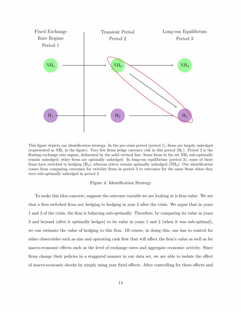
For all these reasons, one can expect inertia at firms with respect to their hedging decisions
in the immediate aftermath of the switch to a floating exchange rate regime. That is, even firms
that should optimally be hedging will take some time to start a hedging program. Consider a
firm that switches from not hedging to hedging within a few years of the regime change. One can
treat outcomes of the same firm before it started to hedge, but after the regime has changed, as a
counterfactual for the same outcomes after the firm started to hedge. The identification strategy
is schematically represented in Figure 4.
13
Fixed Exchange
Rate Regime
Period 1
NH1
H1
Transient Period
Period 2
NH2
H2
Long-run Equilibrium
Period 3
NH3
H3
This figure depicts our identification strategy. In the pre-crisis period (period 1), firms are largely unhedged(represented as NH1 in the figure). Very few firms hedge currency risk in this period (H1). Period 2 is thefloating exchange rate regime, delineated by the solid vertical line. Some firms in the set NH2 sub-optimallyremain unhedged; other firms are optimally unhedged. In long-run equilibrium (period 3), some of thesefirms have switched to hedging (H3), whereas others remain optimally unhedged (NH3). Our identificationcomes from comparing outcomes for switcher firms in period 3 to outcomes for the same firms when theywere sub-optimally unhedged in period 2.
Figure 4: Identification Strategy
To make this idea concrete, suppose the outcome variable we are looking at is firm value. We see
that a firm switched from not hedging to hedging in year 3 after the crisis. We argue that in years
1 and 2 of the crisis, the firm is behaving sub-optimally. Therefore, by comparing its value in years
3 and beyond (after it optimally hedges) to its value in years 1 and 2 (when it was sub-optimal),
we can estimate the value of hedging to this firm. Of course, in doing this, one has to control for
other observables such as size and operating cash flow that will affect the firm’s value as well as for
macro-economic effects such as the level of exchange rates and aggregate economic activity. Since
firms change their policies in a staggered manner in our data set, we are able to isolate the effect
of macro-economic shocks by simply using year fixed effects. After controlling for these effects and
14
other observable differences, a firm fixed effect regression model allows us to estimate the causal
effect of hedging on firm value.
It is worth noting the difference between a fixed effects model in our analysis and such a model
estimated when firms are all in equilibrium. If firms are always in a long-run equilibrium, even
a fixed effects model will not capture any causal effect of hedging. In long-run equilibrium, if a
firm switches from not hedging to hedging, there must have been an underlying change in the cost
and benefit of hedging for that firm. We argue that in our framework, firms are temporarily in
disequilibrium due to the nature of the exogenous shock represented by the switch to the floating
exchange rate regime. Therefore, we can interpret the coefficient in a fixed-effects regression model
as capturing the causal effect of hedging on firm outcomes.
One concern with our identification strategy may be the possibility of a concomitant change
in managers at a firm in the same period that it starts to hedge. If this happens, the effect on
the outcome variable may be due to the superior quality of new management rather than to the
hedging decision. To alleviate this concern, we collect data on CEO changes for all hedger firms in
our sample, and directly include the effect of managerial changes in the regression model.
3 Data and Hedging Determinants
We collect data from two sources. First, we obtain financial statement and market value information
for all Brazilian firms listed in the Economatica database as of August, 2006. This comprises a
list of more than 350 firms. The database over-represents large firms and potentially suffers from
a survivorship bias: we have no data on firms that may have gone bankrupt or been acquired. If
non-hedgers are more likely to fail, the bias works against our finding any positive effects of hedging.
We exclude financial firms, which may use currency derivatives to hedge operational rather than
financial risk. We also exclude state-owned and foreign-owned firms, both of which have potential
access to capital from owners with deep pockets. For each of the firms listed in the database,
we obtain annual financial statements and end-of-year equity market values for the period 1997
through 2005 from Economatica.
15

While Economatica computes equity market values for many firms, there are several missing
values. As a second way of determining equity values, we also determine for each firm and each
class of share it has issued, the average daily closing price for the last five trading days of each year.
We then determine the value of each class of share for each firm by multiplying the average price
with the number of shares outstanding, and add across the classes to determine the overall market
value of equity for the firm. As a cross-check, we find a very high correlation between the market
values from the two methods, when both are available.
Our second source of data is BOVESPA, the Sao Paolo stock exchange. The BOVESPA web site
provides the footnotes to the annual financial statements over our period of study. Since the sets of
firms listed in Economatica and BOVESPA are different, our overall dataset is the intersection of
these two sources of information. We obtain the following items of information for each firm-year
from the footnotes to the balance sheet: whether a firm uses foreign exchange derivatives, whether
it is an exporter, whether it has dollar assets, and the amount of foreign debt outstanding.
Following regulation CVM No. 235, introduced on March 23, 1995, a publicly-traded company
in Brazil is required to disclose whether it uses derivative contracts, and also the nature and face
value of the contracts in the footnotes to the balance sheet.3 Most of the non-users explicitly
mention that they do not use derivatives, whereas many firms do not mention derivatives at all.
The latter are treated as missing values. Since we only know the kinds of derivative contracts used
(e.g., exchange rate or currency derivatives, and swaps, options, or forward contracts) and their
notional value, but not the terms of the contracts themselves, we create a dummy variable dderiv
set to 1 if firms use foreign exchange derivatives, and zero otherwise. The most common hedge
contracts among firms in our sample are currency swaps and forward contracts. In both cases, firms
buy the foreign currency (typically US dollars, and sometimes euro or yen) and pay reais, and are
therefore hedging against a fall in value of the real.
Similarly, we create a dummy variable export set to 1 if a firm is an exporter, and zero otherwise.
Some firms disclose data on exports as part of their annual reports. In other cases, firms mention3The CVM is the Brazilian equivalent of the SEC in the US. We provide an example of our data collection process
in the Appendix.
16
that they are exporters but do not disclose information about foreign sales. The export dummy
is set to 1 in each case. We also create a dummy variable dol set to 1 if a firm holds assets
denominated in or indexed to US dollars. Such assets include cash and deposits in foreign currency
and government bonds (treasury notes and central bank bonds indexed to the dollar). Finally,
in many cases, firms report the currency composition of their debt, from which we determine the
foreign to total debt ratio for each firm.
Our basic measure of value is Tobin’s q, or the ratio of a firm’s market value to its book value,
where market value is determined as the sum of book value of debt and market value of equity,
and book value is the sum of book value of debt and book value of equity. We remove observations
with missing values for market value of equity, book equity, cash holdings, and derivative usage.
Our final data set is an unbalanced panel containing 167 firms, 9 years, and 1,268 observations
(firm-year pairs). We winsorize all variables in both tails at the 1% level to control for outliers.
Table 1 presents the key descriptive statistics for our sample. Panels A and B provide the mean,
median and standard deviation of firm characteristics for hedgers and non-hedgers respectively,
and Panel C provides the corresponding statistics for all firms. Hedgers are much larger than
non-hedgers, both in terms of their revenue and market capitalization. The median hedger firm’s
revenue (R$ 1,534 million) is about six times higher than that of the median non-hedger firm (R$
250 million). The hedger firm’s book leverage (33.16%) is about 12% higher than that of the
median non-hedger firm (20.67%). Noticeably, while the domestic leverage (i.e., the ratio of local
currency debt to book value of assets) is similar at about 10% for the median firm across the two
groups, hedgers have a substantially higher foreign currency leverage, defined as the ratio of foreign
currency debt to book value of assets (19.13% for hedgers versus 3.59% for non-hedgers). The
differences in firm size, book leverage and foreign leverage across the two groups are all significant
at the 1% level. Further, we find that hedgers keep significantly higher cash-balances as compared
to non-hedgers.
We find that hedgers have a net income to assets ratio approximately double that of non-
hedgers, and a capital expenditure to assets ratio almost 50% higher than non-hedgers. Finally,
we find that the median market-to-book ratio for hedgers is 1.09 as against 0.72 for the median
17
non-hedger firm. This difference is significant at the 1% level.
Overall, our univariate results show that hedgers are large firms with high leverage, in particular
with large quantities of foreign currency debt. They are able to invest larger amounts in capital
expenditure. In addition, their market value is significantly higher compared to their non-hedger
counterparts.
3.1 Determinants of Hedging Policy
For our empirical exercise to be meaningful, it is important that there is some evidence of inertia
in firms’ hedging policies. In particular, it is important to provide evidence consistent with the
presence of fixed costs in learning about hedging policies or in starting a hedging program. While it
is difficult to provide direct evidence for such costs, we offer several pieces of background information
and empirical evidence to support our underlying assumption.
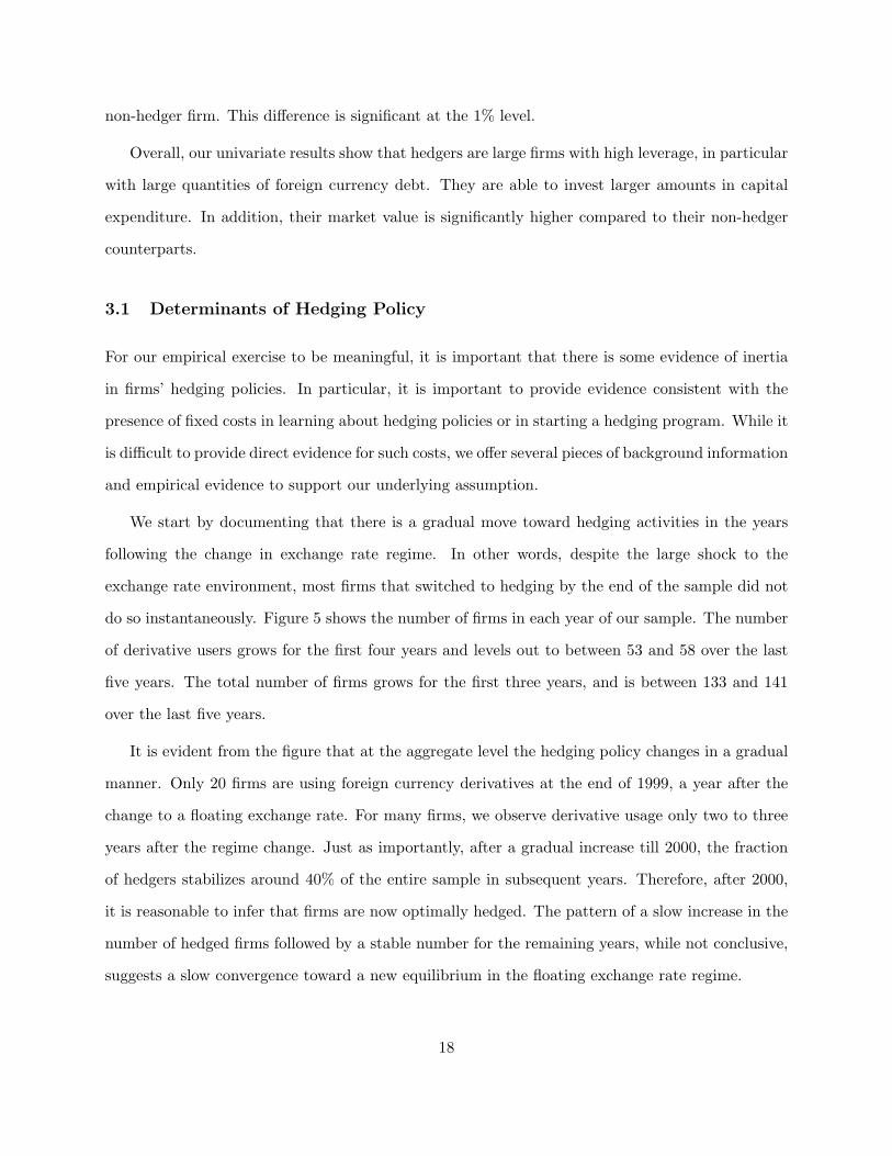
We start by documenting that there is a gradual move toward hedging activities in the years
following the change in exchange rate regime. In other words, despite the large shock to the
exchange rate environment, most firms that switched to hedging by the end of the sample did not
do so instantaneously. Figure 5 shows the number of firms in each year of our sample. The number
of derivative users grows for the first four years and levels out to between 53 and 58 over the last
five years. The total number of firms grows for the first three years, and is between 133 and 141
over the last five years.
It is evident from the figure that at the aggregate level the hedging policy changes in a gradual
manner. Only 20 firms are using foreign currency derivatives at the end of 1999, a year after the
change to a floating exchange rate. For many firms, we observe derivative usage only two to three
years after the regime change. Just as importantly, after a gradual increase till 2000, the fraction
of hedgers stabilizes around 40% of the entire sample in subsequent years. Therefore, after 2000,
it is reasonable to infer that firms are now optimally hedged. The pattern of a slow increase in the
number of hedged firms followed by a stable number for the remaining years, while not conclusive,
suggests a slow convergence toward a new equilibrium in the floating exchange rate regime.
18

0
20
40
60
80
100
120
140
1997 1998 1999 2000 2001 2002 2003 2004 2005
No.o
f firm
s
Year
Derivative Users
Non-Users
This figure shows the numebr of firms in the sample in each year. The number of currency derivative usersincreases gradually until 2001, and then levels off for the remaining years in the sample.
Figure 5: Number of firms in sample
For each firm, its decision to hedge currency risk must be based on its own costs and benefits of
hedging. A firm that faces a relatively minor cost or has a relatively high benefit from hedging is
likely to begin hedging more quickly than other firms. We now present evidence consistent with the
view that firms with higher net benefits, measured as of the beginning of the crisis, started their
hedging programs early. However, the switch was not instantaneous. The intensity of switching
was high in initial years, reaching a peak around 2001 after which it declined.
We consider four proxy variables for the costs and benefits of hedging. For each proxy, we divide
firms into two groups, high and low, depending on whether they fall above or below the sample
median. The variables are all measured as of December, 1998; i.e., before the real is floated, and so
before the full effect of the crisis is felt by sample firms. We compute the estimated hazard rate for
currency derivative use for the two groups based on each proxy using the Nelson-Aalen estimator
for hazard function. The hazard rate function provides the probability of using derivatives in the
next period conditional on remaining unhedged till that point. We expect to observe a steeper
hazard function (i.e., a higher probability of using derivatives in earlier years) for firms that face
below median costs to hedging and obtain above median benefits from hedging.
19

Our first proxy for the cost of hedging is simply a firm’s size in 1998 (as measured by total
assets). To the extent that there are fixed costs to establishing a hedging program, larger firms
should find it advantageous to start hedging earlier. Second, we consider the amount of foreign
currency debt (scaled by total assets) on a firm’s balance sheet in 1998. A firm with substantial
foreign currency debt has greater benefits from currency hedging. In addition, it is more likely to
have an institutional knowledge and manpower in the area of foreign currency management. Third,
we consider the reliance on foreign currency debt for capital expenditure. Specifically, we consider
the ratio of capital expenditure in 1998 to new foreign currency debt in 1998. A firm that relies
extensively on foreign currency debt to fund capital expenditure has greater benefits to hedging.
Finally, we compute the ratio of capital expenditure to total assets in 1998. This ratio proxies for
the investment needs of the firm. A firm with high investment needs will have a greater benefit
from hedging.
We plot the four sets of hazard functions in Figure 6. On the X-axis, time is measured in years
since 1997. For each of our four measures, there is a clear distinction between the two sets of
hazard rate functions. The probability of starting a hedging program is unambiguously higher for
firms that are likely to face lower costs and/or higher benefits from hedging. Further, in each case
the hazard rate function is steeper for firms with lower costs or higher benefits to hedging. This
suggests that the rate at which firms learn about the net benefits of hedging depends on the size
of those benefits.
We re-emphasize that most of our hedged firms do not instantaneously switch from an unhedged
to a hedge state. In all our plots, the hazard rate peaks around year four; i.e., in 2001. After that,
it declines across all four measures. Thus, after the real is floated, many firms begin to hedge in
the subsequent years. The rate at which firms switch from not hedging to hedging increases over
time. Further, this rate is clearly faster for firms with a higher net benefit to hedging.
Overall, our non-parametric results provide support for the key identifying assumption that it
takes firms some time to learn the optimal policy in the new exchange rate regime. We supplement
this exercise with a parametric regression. We model a firm’s decision to start hedging as a function
of its characteristics measured as of the beginning of the year, as well as relevant characteristics
20
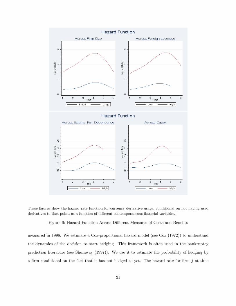
These figures show the hazard rate function for currency derivative usage, conditional on not having usedderivatives to that point, as a function of different contemporaneous financial variables.
Figure 6: Hazard Function Across Different Measures of Costs and Benefits
measured in 1998. We estimate a Cox-proportional hazard model (see Cox (1972)) to understand
the dynamics of the decision to start hedging. This framework is often used in the bankruptcy
prediction literature (see Shumway (1997)). We use it to estimate the probability of hedging by
a firm conditional on the fact that it has not hedged as yet. The hazard rate for firm j at time
21

t (i.e., the probability that firm j at time t will use currency derivatives conditional on it being a
non-user so far) is modeled as:
h(t|xj) = h0(t)exp(xj,t−1βj + xj,1998βj,1998).
Here, xj,t−1 refers to a vector of firm characteristics at the end of year t − 1 that are likely to be
associated with the decision to hedge in year t. h0, called the baseline hazard function, represents
the hazard ratio for a hypothetical firm that assumes a value of zero uniformly for all xj . The
model is estimated via maximum likelihood to obtain the β coefficients.
Here, xi,1998 is a vector of firm characteristics measured as of 1998. The characteristics include
a firm’s size (measured as the natural logarithm of total assets) as a proxy for the economies of
scale in hedging. In other words, this variable is inversely related to the likely cost of starting
a hedging program after the shock. In addition, we include a measure of the firm’s exposure to
foreign currency risk in the floating exchange rate regime. Specifically, we consider each firm’s
foreign currency debt to total asset ratio as of 1998 to proxy for the potential exposure to risk once
the real is floated. This variable proxies for the likely benefits of hedging in the floating exchange
rate regime.
In the model, we include several other firm characteristics measured as of the beginning of
the current year t. The control variables are motivated by prior empirical work on hedging by
non-financial firms.4 The variables include the leverage ratio (i.e., the ratio of debt to firm value),
as firms with greater leverage may be exposed to greater financial distress, and hence have a
stronger motive to hedge. The decision to hedge may be concave in leverage: firms with very high
leverage may have no incentive to hedge even when faced with higher expected bankruptcy costs
(see Purnanandam, 2008). We therefore include the square of the leverage ratio as an explanatory
variable. Among other variables, the firm’s annual capital expenditure captures the effects of
growth opportunities in the spirit of FSS (1993). Finally, we include a dummy variable based on
whether the firm has dollar assets, and a dummy variable based on whether the firm has exports,4See, for example, Geczy, Minton and Schrand (1997), Purnanandam (2008), or Bartram, Brown, and Fehle (2007).
Rossi (2007) studies the determinants of hedging policies of Brazilian firms in a similar time period as ours.
22

to account for natural hedges the firm may have. For this estimation, all variables in levels (such
as firm size and leverage) are measured as of the beginning of the year. Thus, the results can be
interpreted to be predictive.
Table 2 presents the estimation results. In Model 1, we confirm our key results from the non-
parametric analyses. Considering 1998 values, larger firms and firms with a higher foreign leverage
ratio are more likely to begin hedging. In Model 2, we predict the hedging decision based solely
on contemporaneous changes in a firm’s financial conditions and find that larger firms and firms
with a high capital expenditure are more likely to use derivatives. We find a strong non-monotonic
relation between leverage and derivative usage. Overall, the relationship between contemporaneous
firm characteristics and a Brazilian firm’s decision to hedge is similar to what other authors have
found for US firms. In Model 3, we include both the 1998 characteristics of size and foreign
leverage and the contemporaneous variables included in Model 2. Strikingly, we find that even
after controlling for time-varying firm-specific covariates, the size and foreign leverage of the firm
in 1998 predict the hazard rate. In fact in this model, a firm’s 1998 size and foreign leverage are
the only variables other than leverage that are statistically significant in predicting the likelihood
that a firm will start hedging.
Of course, the 1998 values of these variables are likely to be correlated with time-varying
financial characteristics. However, it is clear that a firm’s decision to hedge even a few years after
the regime change is strongly predicted by the relative costs and benefits of hedging as of December
1998. That is, initial conditions just before the switch to floating exchange rates have a lasting
impact, so that a significant part of the motivation to hedge comes from a perturbation in the net
cost of remaining unhedged as a result of the switch to a floating exchange rate. Changes in this
net cost beyond 1998 have very little explanatory power in the hazard rate model. This evidence
is consistent with the presence of set-up or fixed costs to starting a hedging program. The likely
sub-optimality of hedger firms before they begin to hedge then allows us to draw a causal link
between hedging and firm-level outcomes.
23

4 Results on Capital Expenditure, Foreign Currency Debt and
Firm Value
We now turn to a more formal analysis to study the effect of derivative usage on capital expenditure,
foreign currency debt, and firm value.
4.1 Effect of derivatives on capital expenditures
In line with the theoretical arguments of FSS, we estimate the following model to study the effect
of derivatives on capital expenditure:
log(capex)it = α+ β ∗ logtai,t−1 + µ ∗ indmtb−it + γ ∗ dderivit + (2)
ξ ∗ logcashflowit + φ ∗ logcashflowit × dderivit + θ ∗ newceoit + δt + εit
Here, the dependent variable log(capex)it is the natural logarithm of capital expenditure by firm i
in year t. The explanatory variables are the log of total assets of firm i at the beginning of year t
(logtai,t−1), the average market-to-book value of all other firms in the same industry except firm i
at the end of year t (indmtb−it), a dummy variable that takes value 1 if firm i used foreign currency
derivatives in year t (dderivit), the cash flow generated by firm i in year t (cashflowit) and the
interaction of cash flow at time t with the derivative dummy. We also include year fixed effects
to control for the effect of macro-economic conditions such as the GDP growth rate and inflation
levels. While our main focus is on the firm fixed effect estimation results, for completeness we also
estimate this model without the inclusion of firm fixed effects.
We use the log of capital expenditure as our dependent variable, and the log of total assets as a
measure of firm size. This specification allows for variable returns to scale. A coefficient of less than
one on log total assets, for example, indicates decreasing returns to scale. An alternative regression
specification would be to use the ratio of capital expenditure to total assets as the dependent
variable, which implicitly assumes constant returns to scale in the production function. Our results
remain qualitatively similar, though weaker, under this alternative specification.
24
The investment of a firm depends on its investment opportunities. As a proxy for the investment
opportunity set of firm i, we use the average market-to-book ratio of all firms in the industry at
the end of the year, excluding the market-to-book ratio of firm i itself. The market-to-book ratio
at the industry level changes across years, so allows us to control for variation in the industry’s
investment opportunity set across time.5
The hedging variable of interest, dderivit, is an indicator variable that equals one if firm i used
foreign currency derivatives in year t, and zero otherwise. We include an indicator variable newceoit
that equals one if hedged firm i hired a new CEO in year t, and zero otherwise. We do so to ensure
that our results are not driven by a change in the CEO precisely at the time when the firm starts
to hedge.
The cash flow variable takes the firm’s profits before taxes and adds back depreciation and
amortization and net financial expenses. This measure captures the effect of all operating cash
flows, but omits the cash flows from derivatives. We use the natural logarithm of annual cash flows
to reduce skewness in the data. Several firms have negative cash flows in our sample. We scale
all annual cash flows up by adding one plus the negative value of the minimum cash flows across
the entire sample. This transformation allows us to estimate regression model using log(cash flow)
for all firms. We also estimate the model using raw cash flow numbers, and show that our results
remain unchanged.
Table 3 presents the estimation results. Models 1 through 3 are estimated without firm fixed
effects, whereas Models 4 through 6 include these effects. In line with our univariate results, we find
that derivative usage allows firms to invest more (Models 1 through 3). Given our identification
strategy, in the rest of this section we discuss the fixed effect estimation results.
In Model 4, which does not include the cash flow as a dependent variable, we find a positive
coefficient of 0.15 on the dderiv dummy. However, the coefficient is statistically insignificant at the
10% level, with a p-value of approximately 16%. Other results suggest that larger firms and firms
with better investment opportunities invest more. As expected, the coefficient on log total assets5Our results remain unchanged using other proxies for the firm’s investment opportunity set, including the market-
to-book ratio of firm i itself, the sales growth rate of firm i, and an industry market-to-book ratio that does not excludefirm i.
25
is less than one, and is approximately 0.75 across models 4 through 6.
Model 5 presents our base result on derivative usage and capital expenditure. We include
both the logcashflow variable and its interaction with dderiv on the right hand side. There are
three main results based on this estimation. First, we find a positive and statistically significant
coefficient on the derivative dummy: thus, absent any cash flow effects, hedged firms are able to
invest more. Second, we find that firms with higher operating cash flows invest larger amounts.
The elasticity of capital expenditure to internal cash flow is directly given by the coefficient on
the log of cash flow, which is about 0.15 in Model 5. This finding is consistent with a number of
studies based on U.S. data that show that a firm’s investment responds positively to its internal
cash flow. Third, the coefficient on the interaction of cash flow and derivative usage is negative
and significant. That is, the investment of a derivative user is less sensitive to its operating cash
flow than the investment of a non-user, as predicted by the FSS model. In terms of the economic
magnitude, we find that the elasticity of investment to operating cash flow drops by about 0.11 for
derivative users. The sum of the coefficients on the log cash flow variable and its interaction with
dderiv is statistically zero. That is, in our sample hedgers are able to completely insulate their
investment from variability in operating cash flow.
As a robustness exercise, in Model 6 we estimate the firm fixed effect model using the level of
operating cash flow without taking a log transform. Our results remain the same. The estimated
coefficients now measure the percentage increase in capital expenditure for a one-million reais
increase in operating cash flow. We find that if operating cash flow is higher by one million reais,
the log of capital expenditure at a firm increases by about 0.47. That is, capital expenditure itself
increases by a factor of 1.6 (that is, e0.47), or 60%. However, derivative usage completely offsets this
effect as evident by a coefficient of -0.44 on the interaction term. Again, the sum of the coefficients
on cash flow and its interaction with derivative usage is statistically indistinguishable from zero.
There are at least two channels (not mutually exclusive) through which hedging can decrease
the investment-to-cash-flow sensitivity of a firm. First, hedging decreases the variability in a firm’s
overall (operating plus financial) cash flows, which in turn allows the firm to invest smoothly over
time. Second, in part due to the decline in cash flow volatility, hedgers can boost their debt capacity
26

and borrow more from their lenders. We provide direct evidence in support of the increased debt
capacity channel in the next section. Here, we explore the first channel, i.e., whether a firm’s cash
flows become less variable after it starts using currency derivatives.
We measure the variability of net cash flow by its coefficient of variation (COV), i.e., as the
ratio of the standard deviation of net cash flow to the mean net cash flow of the firm. For every firm
that began using foreign currency derivatives in our sample, we compute this number separately for
non-hedger and hedger years. We require a firm to be present for at least six years in our sample
to be included in this exercise. Given the relatively short panel we have, our estimates of volatility
in cash flow are not very precise. Therefore, we consider this exercise to be a supporting piece of
evidence rather than a direct test of volatility reduction. We are able to compute the coefficient of
variation of net cash flow before and after the firm begins hedging for 48 firms. Figure 7 presents
the distribution of their COV during the pre- and post-hedging periods. The COV for the average
firm declines from 1.78 to 1.27 after it starts to hedge. The difference is significant at the 1%
significance level (t-stat=3.11).
It is important to note that the Brazilian economy stabilizes considerably during the latter half
of our sample period. This stability in turn leads to an overall decline in volatility of output and
prices. By construction, the observations in which a firm uses derivatives fall in the latter half
of the sample period. Therefore, the decline in COV documented above need not be caused by
derivative usage.
To account for the overall reduction in volatility, we compute the COV for all firms that remained
unhedged throughout the sample period. Figure 7 also presents the distribution of COV for this
control sample, before and after 2001. It is evident that unhedged firms also experienced a decline
in volatility of net cash flow in the second half of the sample period. However, the rate of decline is
much steeper for derivative users. The decline in COV is 0.50 (or 28% from the pre-hedging value)
for hedged firms, as compared to a decline of 0.08 (or 6% from pre-2001 values) for non-hedgers.
After a test of the difference in these two differences, we reject the null hypothesis that there was
an equal decline in COV across the two samples. Our results are unchanged if we use either 2000
or 2002 as a cutoff year for unhedged firms. Overall, the results on reduced variability of cash flows
27

These figures show the coefficient of variation (i.e., the standard deviation scaled by the mean) in net cashflow for hedger firms (left figure) and firms that remain unhedged by the end of the sample period (rightfigure). The figure on the left shows that the volatility in net cash flow is lower for hedgers after they beginto hedge. The figure on the right shows that the volatility in cash flow is lower for non-hedgers as well after2001. However, the decline is steeper for hedged firms.
Figure 7: Coefficient of variation in net cash flow for hedger and non-hedger firms
are consistent with the theoretical predictions of FSS and with our results relating investment to
cash flow. The results also confirm that in our sample, firms that use derivatives do so to hedge
their cash flow risk, rather than simply to speculate.
4.2 Foreign currency debt
As discussed in Section 2.2, Leland (1998) shows that hedging can add value by increasing the debt
capacity of a firm. Recall from Section 2.1 that, at the macroeconomic level there is evidence that
(a) domestic credit was scarce in Brazil during the period of study, and (b) domestic interest rates
were very high during this period. Thus, if hedging increases the access to foreign debt, firms can
benefit both via greater quantity and reduced cost of debt financing.
We first test whether derivative usage allows firms to raise more debt financing by estimating
28
the following model:
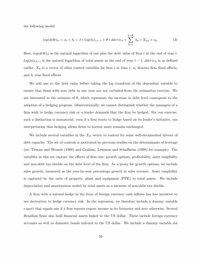
log(debt)it = αi + δt + β ∗ log(ta)i,t−1 + θ ∗ dderivit +k=K∑k=1
βki ∗Xkit + εit. (3)
Here, log(debt)it is the natural logarithm of one plus the debt value of firm i at the end of year t,
log(ta)i,t−1 is the natural logarithm of total assets at the end of year t − 1, dderivit is as defined
earlier, Xit is a vector of other control variables for firm i at time t, αi denotes firm fixed effects,
and δt year fixed effects.
We add one to the debt value before taking the log transform of the dependent variable to
ensure that firms with zero debt in any year are not excluded from the estimation exercise. We
are interested in the estimate of θ, which represents the increase in debt level consequent to the
adoption of a hedging program. Observationally, we cannot distinguish whether the managers of a
firm wish to hedge currency risk or a lender demands that the firm be hedged. For our exercise,
such a distinction is immaterial: even if a firm starts to hedge based on its lender’s initiative, our
interpretation that hedging allows firms to borrow more remains unchanged.
We include several variables in the Xit vector to control for some well-documented drivers of
debt capacity. The set of controls is motivated by previous studies on the determinants of leverage
(see Titman and Wessels (1988) and Graham, Lemmon and Schallheim (1998) for example). The
variables in this set capture the effects of firm size, growth options, profitability, asset tangibility
and non-debt tax shields on the debt level of the firm. As a proxy for growth options, we include
sales growth, measured as the year-by-year percentage growth in sales revenue. Asset tangibility
is captured by the ratio of property, plant and equipment (PPE) to total assets. We include
depreciation and amortization scaled by total assets as a measure of non-debt tax shields.
A firm with a natural hedge in the form of foreign currency cash inflows has less incentive to
use derivatives to hedge currency risk. In the regression, we therefore include a dummy variable
export that equals one if a firm reports export income in its footnotes and zero otherwise. Several
Brazilian firms also hold financial assets linked to the US dollar. These include foreign currency
accounts as well as domestic bonds indexed to the US dollar. We include a dummy variable dol
29
that equals one for firms with dollar assets and zero otherwise.
In our first exercise we estimate this model with foreign currency debt as the dependent variable.
Model 1 of Table 4 provides the regression estimates. The coefficient θ on the dderiv variable is
0.8951. Therefore, the a firm’s total foreign debt increases by about 145% (i.e., approximately
e0.8951−1) after it starts using currency derivatives. The result is significant at 1% level. Consistent
with the notion that the extra debt is used to fund capital expenditure, we find a positive and
statistically significant coefficient on the depreciation expense variable.
In Model 2 of the table, we replace foreign debt with domestic debt as the dependent variable,
and show that the adoption of a hedging program has no meaningful effect of domestic borrowing.
Thus, the increase in foreign debt is not merely a replacement of domestic currency debt. Recall that
univariate results in Table 1 also confirm this result: while hedgers have significantly higher foreign
leverage as compared to non-hedgers, both the groups have similar levels of domestic leverage. In
unreported tests we also regress total debt of the firm on dderiv and find a positive and significant
coefficient. In Models 3 and 4 of Table 4, we regress the ratio of foreign currency debt to total debt
on the explanatory variables. In both models, we find that larger firms have a greater proportion
of foreign debt. The coefficient on derivative usage is also positive and significant in both models.
Taken together these results suggest that using currency derivatives allows firms to increase
their foreign currency debt. The access to foreign capital is especially important at a time when
capital in the domestic economy is scarce. Overall, derivative usage allows a firm to invest both
by decreasing the volatility of internal cash flows and by allowing it to raise more capital in the
external market. We conclude our analysis by investigating the effect of these factors on the overall
value of the firm.
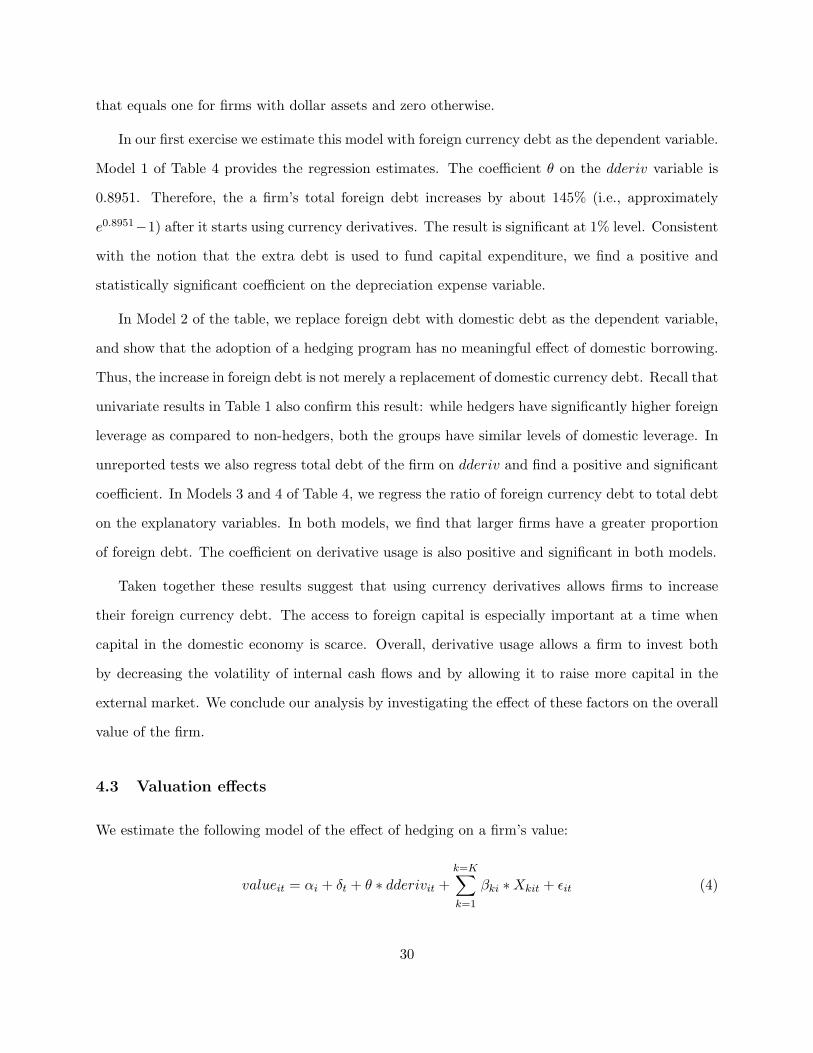
4.3 Valuation effects
We estimate the following model of the effect of hedging on a firm’s value:
valueit = αi + δt + θ ∗ dderivit +k=K∑k=1
βki ∗Xkit + εit (4)
30

The dependent variable, valueit, is the Tobin’s q of firm i at time t. The explanatory variables
include firm fixed effects (αi), year fixed effects (δt), a derivative usage dummy set to 1 if firm i
uses foreign currency derivatives in year t (dderivit), and a vector of control variables for firm i at
time t (Xit).
Xit includes the following control variables. We use the log of total revenue to proxy for firm
size.6 A dummy variable newceoit is set to 1 if firm i changed its CEO in year t. The growth in
sales revenue from time t − 1 to t is used as a measure of growth rate. We include a proxy for
the firm’s profitability, margin, measured as the ratio of earnings before interest and taxes (EBIT)
to total assets. The ratio of capital expenditures to total assets proxies for current investment
opportunities. We also include the ratios of financial income to total assets and financial expenses
to total assets as measures of financial cash flow variables that may affect value. As access to
foreign debt is likely to be valuable for Brazilian firms in these crisis years, we include the ratio
of foreign currency debt to total debt. Finally, we include dummy variables for firms that have
dollar assets and firms that have export income. Needless to say, many of these variables are
likely to be correlated with each other as well as correlated with the use of derivatives itself. For
example, we have already shown that derivatives correlate with the foreign currency leverage of
firms. Therefore, to carefully separate their effects on firm value, we include additional regressors
in a step-wise manner in the regression model.
The results are reported in Table 5. As discussed earlier, all models include firm fixed effects and
exploit the variation in firm value as a firm moves from the state of temporary sub-optimality as a
non-hedger to the state of optimal hedger. We find a positive and significant coefficient on dderiv
across all four model specifications in the Table. In terms of economic magnitudes, derivative usage
increases the value of a firm by approximately 10–12%. Statistically, the coefficient is significant at
the 5% level or better in Models 1, 2, and 3, and at the 10% level in Model 4.
In Models 2 and 3, the coefficient on the CEO turnover dummy is significant and negative.
While it is beyond the scope of our investigation, it seems that CEOs are fired in anticipation6Since our dependent variable, Tobin’s Q, includes book value of asset in the denominator, we use revenue as
a proxy for firm size in this model to ensure that our results are not contaminated by any mechanical relationshipbetween the two variables.
31
of poor performance due to their decisions. Size is positively related to value in Model 3, but in
Model 4 it’s effect is dominated by the effects of operating margin and capital expenditure. The
profitability margin of a firm is the most important determinant of its value in our sample as
evidenced by statistically and economically large coefficient on margin in Model 4 of the Table.
Our estimate of the effect of derivative usage on value is approximately twice as high as that
found by Allayannis and Weston (2002), who find that US users of foreign currency derivatives have
a approximately 4.87% higher value than non-users. We emphasize that, given the scale of the crisis
in Brazil during our sample period and the scarcity of domestic capital, currency derivatives are
especially important in our sample because of the access to foreign capital. Guay and Kothari
(2003) suggest that the extent of derivative usage by US firms is too small to justify a value
premium of about 5%. They show via simulation that a simultaneous three standard deviation
adverse change in exchange rates, interest rates, and commodity prices will generate enough cash
flow via derivatives holdings to add only 1.3% to the the equity value of the median US firm. Indeed,
when it is relatively easy for firms to raise external capital, our arguments do not apply and we
should expect to see low value premia. However, when external financing is costly or difficult,
the FSS model implies that hedging will have high value and our empirical exercise confirms this
prediction.
5 Conclusion
The Brazilian currency crisis of 1999 represents a natural setting to study the effects of corporate
financial policy on firm outcomes. The switch to a floating exchange rate in January 1999 was
followed by periods of high volatility and rapid depreciation of the real. We analyze the effect
of risk-management policies in a panel of Brazilian firms from 1998 to 2005. By focusing on an
economy in disequilibrium, we are more likely to establish a causal effect of hedging on firm value.
That is, in a firm-fixed effect specification, we compare a firm that hedges with the same firm when
it was not hedging. If the firm was behaving sub-optimally in the latter case, the difference in
outcomes is attributable to the use of derivatives.
32

We find that foreign currency hedging allows firms to both increase their capital expenditures
and to smooth their investment policies. In particular, hedger firms’ investment is less sensitive to
their operating cash flows as compared to their non-hedger counterparts. Since external financing
is indeed costly for firms in Brazil during our study, our results provide support for the Froot,
Scharfstein and Stein (1993) model. The result that the foreign debt capacity of a firm increases
when it uses derivatives ties into the predictions of Leland (1998).
We find that foreign currency hedging is positively correlated with the value of a firm. In
particular, we estimate a valuation premium in the range of 10–12% for currency hedging by
Brazilian firms in the period of our study. Overall, therefore, we provide evidence that risk-
management policies add significant value to firms during a period of economic turmoil. More
broadly, we show that when there is a supply shock to one source of capital, financial policies that
make it easier to access other sources of capital lead to better real outcomes and increased value
for firms.
33

References
[1] Adam, T., S. Dasgupta, and S. Titman, 2007, Financial Constraints, Competition and Hedgingin Industry equilibrium, forthcoming, Journal of Finance.
[2] Allayannis, G. and J. Weston, 2001, The Use of Foreign Currency Derivatives and Firm MarketValue, Review of Financial Studies 14, 243–276.
[3] Allayannis, G., G. Brown, and L. Klapper, 2002, Capital Structure and Financial Risk:Evidence from Foreign Debt Use in East Asia, Journal of Finance 58(6), 2667–2709.
[4] Arida, P., E. L. Bacha, and A. Lara-Resende, 2005, Credit, Interest, and JurisdictionalUncertainty: Conjectures on the Case of Brazil, in F. Giavazzi, I. Goldfajn, and S. Herrera (eds)Inflation Targeting, Debt, and the Brazilian Experience, 1999 to 2003 , MIT Press, Cambridge,MA.
[5] Averbug, A., 2002, The Brazilian Economy in 1994: From the Real Plan to Inflation Targets,The World Economy 25 (7), 925–944.
[6] Bartram, S., G. Brown, and F. Fehle, 2006, International Evidence on Financial DerivativeUsage, Working paper.
[7] Belaisch, A., 2003, Do Brazilian banks compete? IMF Working Paper 03/113.
[8] Berrospide, J., 2010, Exchange Rates, Optimal Debt Composition and Hedging in Small OpenEconomies, Working paper, Federal Reserve Board of Governors.
[9] Bonomo, M., B. Martins and R. Pinto, 2003, Debt composition and exchange rate balancesheet effect in Brazil, a firm level analysis, Emerging Markets Review 4(4), 368–396.
[10] Campello, M., C. Lin, Y. Ma and H. Zhou. “The Real and Financial Implications of CorporateHedging,” forthcoming, Journal of Finance.
[11] Chava, S. and A. Purnanandam, 2011, The effect of banking crisis on bank-dependentborrowers, Journal of Financial Economics, 99, 116-135.
[12] Cowan, K., E. Hansen and Luis O. Herrera, 2005, Currency Mismatches, Balance Sheet Effectsand Hedging in Chilean Non-Financial Corporations, Central Bank of Chile Working PaperNo. 346.
[13] Cox, D. R, 1972, Regression models and life tables, Journal of the Royal Statistical Society, 34(2), 187-220.
[14] Froot, K., D. Scharfstein, and J. Stein, 1993, Risk Management: Coordinating CorporateInvestment and Financing Policies, Journal of Finance, 48, 1629–1658.
[15] Gelos, R. G., 2006, Banking Spreads in Latin America, The IMF Working Paper, 06/44.
[16] Geczy, C., B. A. Minton and C. Schrand, 1997, Why Do Firms Use Currency Derivatives?Journal of Finance 52, 1323-1354.
34
[17] Graham, John R., and Daniel A. Rogers, 2002, Do Firms Hedge in Response to Tax Incentives?Journal of Finance 57, 815–839.
[18] Guay, W. and S. Kothari, 2003, How Much Do Firms Hedge with Derivatives? Journal ofFinancial Economics 70, 423–461.
[19] Holmstrom, B. and J. Tirole, 1997, Financial Intermediation, Loanable Funds, and the RealSector, Quarterly Journal of Economics 112(3), 663–691.
[20] Jin, Yanbo, and Philippe Jorion, 2006, Firm Value And Hedging: Evidence From U.S. Oil andGas Producers, Journal of Finance 61, 893-919.
[21] Khwaja, A., Mian, A., 2008, Tracing The Impact of Bank Liquidity Shocks: Evidence from anemerging market, American Economic Review 98, 1413-1442.
[22] Leland, H. E., 1998, Agency Costs, Risk Management, and Capital Structure, Journal ofFinance 53, 1213-1243.
[23] Mackay, P. and S. Moeller, 2007, The Vale of Corporate Risk Management, Journal of Finance62, 1379–1419.
[24] Nakane, M., T. Afanasieff and P. V. Lhacer, 2002, The Determinants of Bank Interest Spreadin Brazil, Central Bank of Brazil Working Paper Series, 46.
[25] Paravisini, D., 2008. Local bank financial constraints and firm access to external finance,Journal of Finance 63, 2161-2193.
[26] Petersen, M. and S. Thiagarajan, 2000, Risk Measurement and Hedging, With and WithoutDerivatives, Financial Management 29, 5–30.
[27] Rossi, J. L., 2007, The Use of Currency Derivatives by Brazilian Companies: An EmpiricalInvestigation, Brazilian Review of Finance 5(2), 205–232.
[28] Purnanandam, A., 2008, Financial distress and corporate risk management: Theory &Evidence, Journal of Financial Economics, 87, 706–739.
[29] Rogoff, K., 2005, Strategies for Bringing Down Long-Term Real Interest Rates in Brazil,Central Bank of Brazil Presentation on August 30, 2005.
[30] Smith, C.W., and R. Stulz, 1985, The determinants of firms’ hedging policies, Journal ofFinancial and Quantitative Analysis 28, 391-405.
[31] Sobrinho, N. F. S., 2007, The Macroeconomics of Bank Interest Spreads: Evidence from Brazil,Working Paper, University of California, Los Angeles, Department of Economics.
[32] Stulz, R., 1984, Optimal hedging policies, Journal of Financial and Quantitative Analysis 19,127-140.
[33] Stulz, R., 1996, Rethinking Risk Management, Journal of Applied Corporate Finance 9(3),8–24.
[34] Tufano, P., 1996, Who Manages Risk? An Empirical Examination of Risk ManagementPractices in the Gold Mining Industry, Journal of Finance 51(4), 1097–1137.
35
A Appendix
A.1 Description of Variables
The following variables are defined for each firm and each year.
logsize: natural logarithm of sales revenues.
salesgrowth: growth rate of revenues from year t− 1 to year t.
margin: ratio of EBIT to total assets.
ebitda: ratio of EBITDA to total assets.
dep/TA: ratio of depreciation and amortization to total assets.
ppe/TA: ratio of permanent assets (the bulk of which are plant, property, and equipment) to totalassets.
leverage: ratio of total debt to total assets.
forlev: ratio of foreign currency debt to total assets.
domlev: ratio of domestic currency debt to total assets.
cash: ratio of cash and short-term investments to total assets.
cashflow: operating profit before taxes plus depreciation and amortization plus net financialexpenses.
invinc: income from equity investments in other firms.
dderiv: dummy variable set to 1 if firm uses foreign currency derivatives, and zero otherwise.
export: dummy variable set to 1 if firm reports export sales, and zero otherwise.
dol: dummy variable set to 1 if firm reports foreign currency asset holdings, and zero otherwise.
A.2 Example Firm
To illustrate the data collection process, we consider the firm Acesita S.A. in the year 2001.Financial information (i.e., the balance sheet and income statement) is obtained from Economatica,as is the market value of equity. Most of the variables we need (including, for example, book valueof debt, revenues, net profit) are thus easily obtained.
Data on hedging and the extent of foreign currency debt are in the explanatory notes to thefinancial statements (the “Notas Explicativas”) maintained on the Bovespa (the Sao Paolo stockexchange) web site at www.bovespa.br.
36

From the Notas Explicativas for Acesita S.A. in 2001, we extract the following information:
Item Page Item (in Portuguese) Translation AmountNumber to English (thousands of R$)13. 17–18 Financiamentos Financing
Moeda estrangeira Foreign currency 2,074,809Moeda nacional Domestic currency 330,411
21. 24–26 Instrumentos Financeiros Financial Instruments
Operacoes de Swap Swap operations 995,404
Table A: Information obtained from financial statement notes for Acesita S.A. in 2001
The text on Item 21 (page 25), Instrumentos Financeiros, explains that the firm engagesin currency swap operations to reduce the effects of exchange rate variation. Similarly, the texton page 5 (Item 4, Disponibilidades or Short-term assets) explains that a specified amount of theshort-term assets are indexed to the US dollar.
Based on this information, we set dderiv = 1 (since it has a foreign currency derivativeposition) and dol = 1 (since it holds foreign currency assets) for Acesita in 2001.
37
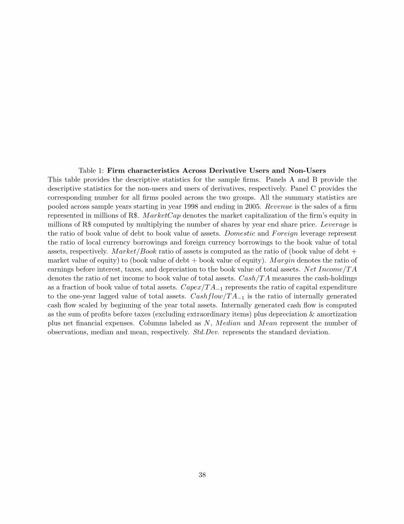
Table 1: Firm characteristics Across Derivative Users and Non-UsersThis table provides the descriptive statistics for the sample firms. Panels A and B provide thedescriptive statistics for the non-users and users of derivatives, respectively. Panel C provides thecorresponding number for all firms pooled across the two groups. All the summary statistics arepooled across sample years starting in year 1998 and ending in 2005. Revenue is the sales of a firmrepresented in millions of R$. MarketCap denotes the market capitalization of the firm’s equity inmillions of R$ computed by multiplying the number of shares by year end share price. Leverage isthe ratio of book value of debt to book value of assets. Domestic and Foreign leverage representthe ratio of local currency borrowings and foreign currency borrowings to the book value of totalassets, respectively. Market/Book ratio of assets is computed as the ratio of (book value of debt +market value of equity) to (book value of debt + book value of equity). Margin denotes the ratio ofearnings before interest, taxes, and depreciation to the book value of total assets. Net Income/TAdenotes the ratio of net income to book value of total assets. Cash/TA measures the cash-holdingsas a fraction of book value of total assets. Capex/TA−1 represents the ratio of capital expenditureto the one-year lagged value of total assets. Cashflow/TA−1 is the ratio of internally generatedcash flow scaled by beginning of the year total assets. Internally generated cash flow is computedas the sum of profits before taxes (excluding extraordinary items) plus depreciation & amortizationplus net financial expenses. Columns labeled as N , Median and Mean represent the number ofobservations, median and mean, respectively. Std.Dev. represents the standard deviation.
38

Firm characteristics Across Derivative Users and Non-UsersVariable N Median Mean Std.Dev.Panel A: Non-UsersRevenue (R$ million) 739 250.3540 547.7564 846.1463MarketCap (R $ million) 739 73.9195 358.4563 978.6524Leverage 739 0.2067 0.2291 0.1782Domestic Leverage 739 0.1048 0.1424 0.1421Foreign Leverage 739 0.0359 0.0867 0.1150Market/Book 739 0.7235 0.8546 0.5454Margin 709 0.1112 0.1185 0.1055Net Income/TA 739 0.0208 0.0209 0.0931Cash/TA 739 0.0312 0.0681 0.0896Capex/TA−1 658 0.0387 0.0534 0.0617Cashflows/TA−1 709 0.1090 0.1152 0.1050Panel B: UsersRevenue (R$ million) 431 1534.7070 3268.7159 4241.5910MarketCap (R$ million) 431 900.4713 2985.3811 4496.1053Leverage 431 0.3316 0.3340 0.1323Domestic Leverage 431 0.1076 0.1270 0.0933Foreign Leverage 431 0.1913 0.2069 0.1250Market/Book 431 1.0938 1.2665 0.6701Margin 421 0.1754 0.1861 0.0906Net Income/TA 431 0.0425 0.0428 0.0714Cash/TA 431 0.0622 0.1049 0.1106Capex/TA−1 402 0.0644 0.0830 0.0699Cashflow/TA−1 421 0.1671 0.1777 0.0904Panel C: All firmsRevenue (R$ million) 1170 512.1240 1550.0928 2965.4466MarketCap (R$ million) 1170 184.0293 1326.1525 3106.0314Leverage 1170 0.2712 0.2678 0.1704Domestic Leverage 1170 0.1065 0.1367 0.1265Foreign Leverage 1170 0.0952 0.1310 0.1321Market/Book 1170 0.8663 1.0063 0.6265Margin 1130 0.1371 0.1437 0.1053Net Income/TA 1170 0.0297 0.0290 0.0863Cash/TA 1170 0.0395 0.0817 0.0994Capex/TA1 1060 0.0477 0.0646 0.0665Cashflow/TA−1 1130 0.1334 0.1385 0.1042
39
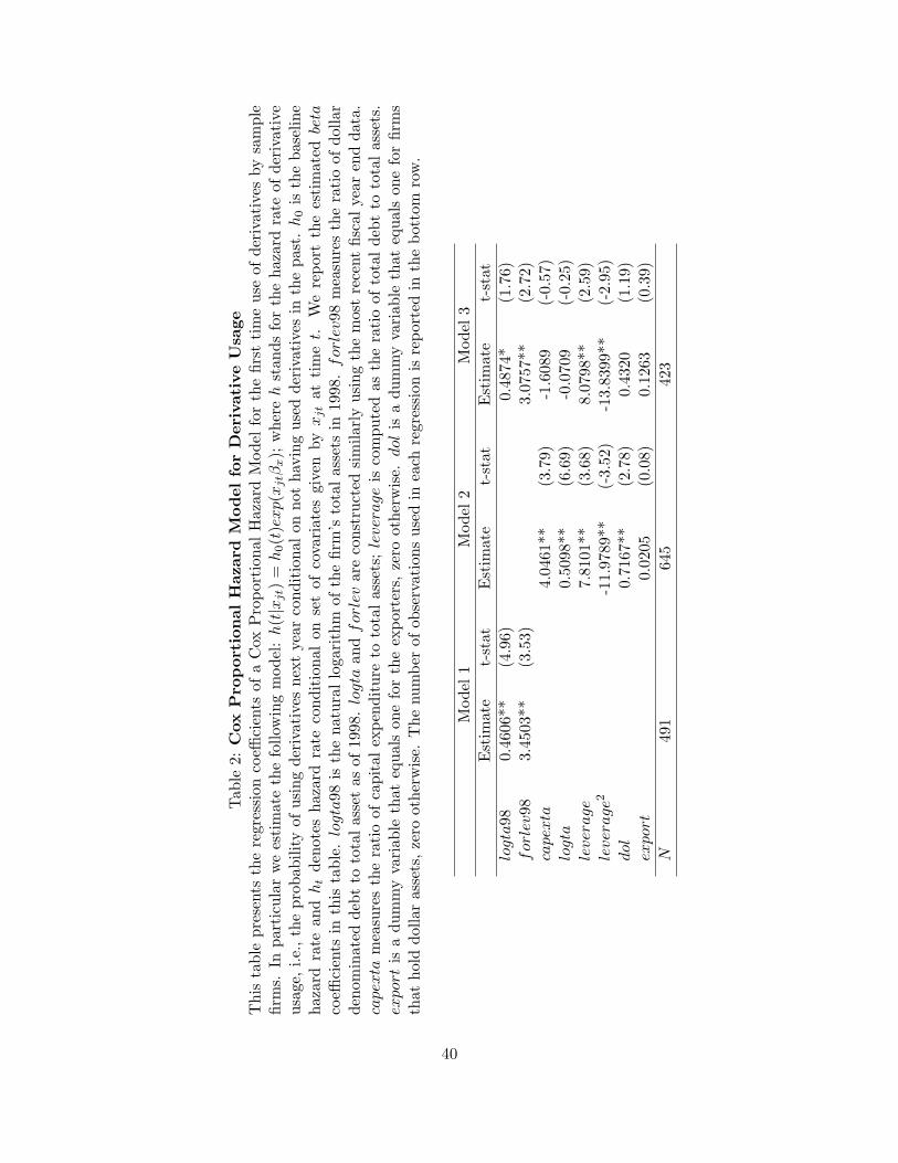
Tab
le2:
Cox
Pro
por
tion
alH
azar
dM
od
elfo
rD
eriv
ativ
eU
sage
Thi
sta
ble
pres
ents
the
regr
essi
onco
effici
ents
ofa
Cox
Pro
port
iona
lH
azar
dM
odel
for
the
first
tim
eus
eof
deri
vati
ves
bysa
mpl
efir
ms.
Inpa
rtic
ular
we
esti
mat
eth
efo
llow
ing
mod
el:h
(t|x
jt)
=h
0(t
)exp(x
jtβ
x);
whe
reh
stan
dsfo
rth
eha
zard
rate
ofde
riva
tive
usag
e,i.e
.,th
epr
obab
ility
ofus
ing
deri
vati
ves
next
year
cond
itio
nal
onno
tha
ving
used
deri
vati
ves
inth
epa
st.h
0is
the
base
line
haza
rdra
tean
dh
tde
note
sha
zard
rate
cond
itio
nal
onse
tof
cova
riat
esgi
ven
byx
jtat
tim
et.
We
repo
rtth
ees
tim
ated
beta
coeffi
cien
tsin
this
tabl
e.logta
98is
the
natu
ral
loga
rith
mof
the
firm
’sto
tal
asse
tsin
1998
.forlev98
mea
sure
sth
era
tio
ofdo
llar
deno
min
ated
debt
toto
tal
asse
tas
of19
98.logta
andforlev
are
cons
truc
ted
sim
ilarl
yus
ing
the
mos
tre
cent
fisca
lye
aren
dda
ta.
capexta
mea
sure
sth
era
tio
ofca
pita
lex
pend
itur
eto
tota
las
sets
;leverage
isco
mpu
ted
asth
era
tio
ofto
tal
debt
toto
tal
asse
ts.
export
isa
dum
my
vari
able
that
equa
lson
efo
rth
eex
port
ers,
zero
othe
rwis
e.dol
isa
dum
my
vari
able
that
equa
lson
efo
rfir
ms
that
hold
dolla
ras
sets
,ze
root
herw
ise.
The
num
ber
ofob
serv
atio
nsus
edin
each
regr
essi
onis
repo
rted
inth
ebo
ttom
row
.
Mod
el1
Mod
el2
Mod
el3
Est
imat
et-
stat
Est
imat
et-
stat
Est
imat
et-
stat
logta
980.
4606
**(4
.96)
0.48
74*
(1.7
6)forlev98
3.45
03**
(3.5
3)3.
0757
**(2
.72)
capexta
4.04
61**
(3.7
9)-1
.608
9(-
0.57
)logta
0.50
98**
(6.6
9)-0
.070
9(-
0.25
)leverage
7.81
01**
(3.6
8)8.
0798
**(2
.59)
leverage2
-11.
9789
**(-
3.52
)-1
3.83
99**
(-2.
95)
dol
0.71
67**
(2.7
8)0.
4320
(1.1
9)export
0.02
05(0
.08)
0.12
63(0
.39)
N49
164
542
3
40
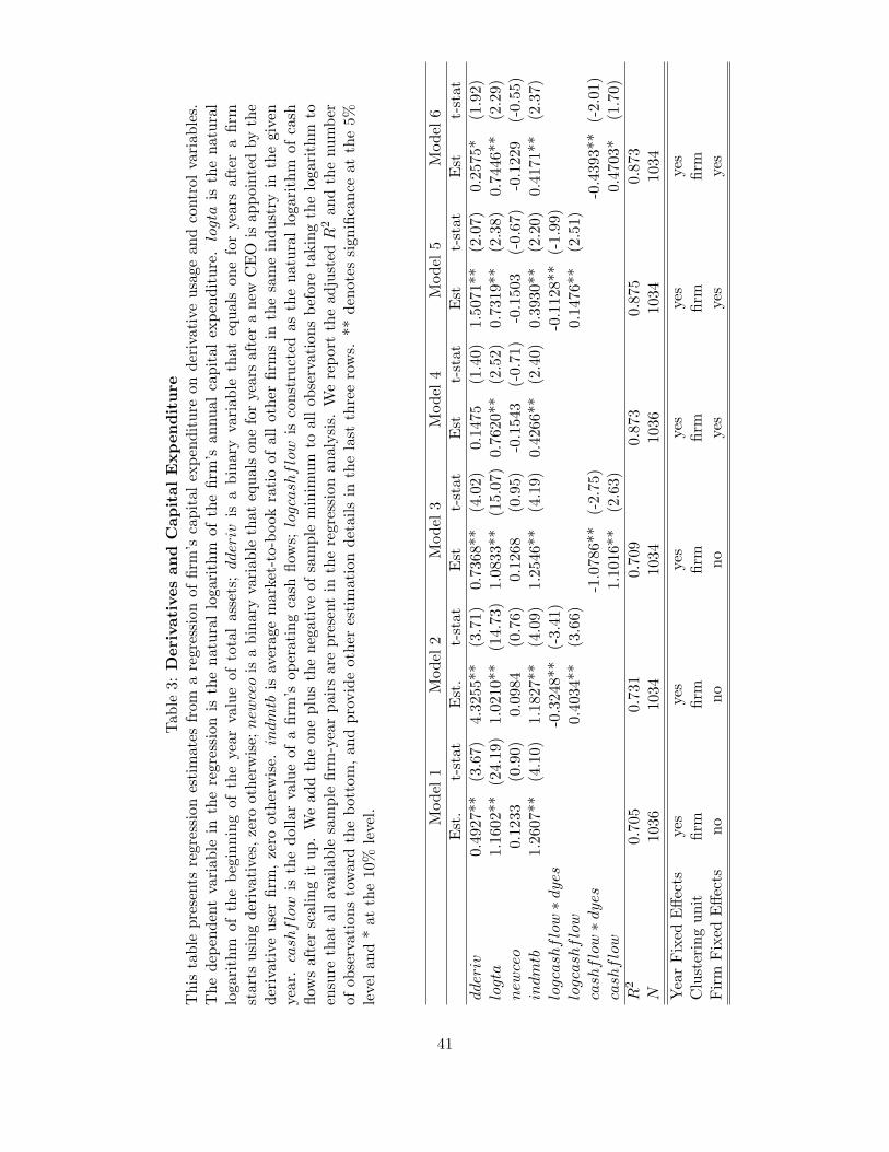
Tab
le3:
Der
ivat
ives
and
Cap
ital
Exp
end
iture
Thi
sta
ble
pres
ents
regr
essi
ones
tim
ates
from
are
gres
sion
offir
m’s
capi
tal
expe
ndit
ure
onde
riva
tive
usag
ean
dco
ntro
lva
riab
les.
The
depe
nden
tva
riab
lein
the
regr
essi
onis
the
natu
ral
loga
rith
mof
the
firm
’san
nual
capi
tal
expe
ndit
ure.
logta
isth
ena
tura
llo
gari
thm
ofth
ebe
ginn
ing
ofth
eye
arva
lue
ofto
tal
asse
ts;dderiv
isa
bina
ryva
riab
leth
ateq
uals
one
for
year
saf
ter
afir
mst
arts
usin
gde
riva
tive
s,ze
root
herw
ise;newceo
isa
bina
ryva
riab
leth
ateq
uals
one
for
year
saf
ter
ane
wC
EO
isap
poin
ted
byth
ede
riva
tive
user
firm
,ze
root
herw
ise.indmtb
isav
erag
em
arke
t-to
-boo
kra
tio
ofal
lot
her
firm
sin
the
sam
ein
dust
ryin
the
give
nye
ar.cashflow
isth
edo
llar
valu
eof
afir
m’s
oper
atin
gca
shflo
ws;logcashflow
isco
nstr
ucte
das
the
natu
ral
loga
rith
mof
cash
flow
saf
ter
scal
ing
itup
.W
ead
dth
eon
epl
usth
ene
gati
veof
sam
ple
min
imum
toal
lob
serv
atio
nsbe
fore
taki
ngth
elo
gari
thm
toen
sure
that
all
avai
labl
esa
mpl
efir
m-y
ear
pair
sar
epr
esen
tin
the
regr
essi
onan
alys
is.
We
repo
rtth
ead
just
edR
2an
dth
enu
mbe
rof
obse
rvat
ions
tow
ard
the
bott
om,
and
prov
ide
othe
res
tim
atio
nde
tails
inth
ela
stth
ree
row
s.**
deno
tes
sign
ifica
nce
atth
e5%
leve
lan
d*
atth
e10
%le
vel. Mod
el1
Mod
el2
Mod
el3
Mod
el4
Mod
el5
Mod
el6
Est
.t-
stat
Est
.t-
stat
Est
t-st
atE
stt-
stat
Est
t-st
atE
stt-
stat
dderiv
0.49
27**
(3.6
7)4.
3255
**(3
.71)
0.73
68**
(4.0
2)0.
1475
(1.4
0)1.
5071
**(2
.07)
0.25
75*
(1.9
2)logta
1.16
02**
(24.
19)
1.02
10**
(14.
73)
1.08
33**
(15.
07)
0.76
20**
(2.5
2)0.
7319
**(2
.38)
0.74
46**
(2.2
9)newceo
0.12
33(0
.90)
0.09
84(0
.76)
0.12
68(0
.95)
-0.1
543
(-0.
71)
-0.1
503
(-0.
67)
-0.1
229
(-0.
55)
indmtb
1.26
07**
(4.1
0)1.
1827
**(4
.09)
1.25
46**
(4.1
9)0.
4266
**(2
.40)
0.39
30**
(2.2
0)0.
4171
**(2
.37)
logcashflow∗dyes
-0.3
248*
*(-
3.41
)-0
.112
8**
(-1.
99)
logcashflow
0.40
34**
(3.6
6)0.
1476
**(2
.51)
cashflow∗dyes
-1.0
786*
*(-
2.75
)-0
.439
3**
(-2.
01)
cashflow
1.10
16**
(2.6
3)0.
4703
*(1
.70)
R2
0.70
50.
731
0.70
90.
873
0.87
50.
873
N10
3610
3410
3410
3610
3410
34Y
ear
Fix
edE
ffect
sye
sye
sye
sye
sye
sye
sC
lust
erin
gun
itfir
mfir
mfir
mfir
mfir
mfir
mF
irm
Fix
edE
ffect
sno
nono
yes
yes
yes
41

Tab
le4:
For
eign
Cu
rren
cyD
ebt-
Mix
and
Der
ivat
ive
Usa
geT
his
tabl
epr
esen
tsfir
mfix
edeff
ect
regr
essi
ones
tim
ates
from
are
gres
sion
offir
m’s
fore
ign
curr
ency
and
dom
esti
cde
bton
deri
vati
veus
age
and
cont
rol
vari
able
s.T
hede
pend
ent
vari
able
isth
ena
tura
llo
gari
thm
ofon
epl
usto
tal
amou
ntof
fore
ign
curr
ency
debt
inM
odel
1.In
Mod
el2,
the
depe
nden
tva
riab
leis
the
natu
rall
ogar
ithm
ofon
epl
usto
tall
ocal
curr
ency
ordo
mes
tic
debt
ofth
efir
m.
Mod
els
3an
d4
use
the
rati
oof
fore
ign
curr
ency
debt
toth
eto
tal
debt
ofth
efir
mas
the
depe
nden
tva
riab
le.dderiv
isa
bina
ryva
riab
leth
ateq
uals
one
for
year
saf
ter
afir
ms
star
tsus
ing
deri
vati
ves,
zero
othe
rwis
e;logta
isth
ena
tura
llo
gari
thm
ofth
efir
m’s
tota
las
sets
asof
the
begi
nnin
gof
the
year
;margin
mea
sure
sth
eop
erat
ing
profi
tof
the
firm
and
isco
nstr
ucte
das
the
rati
oof
earn
ings
befo
rein
tere
stan
dta
xes
toth
ebo
okva
lue
ofto
tal
asse
ts;export
isa
dum
my
vari
able
that
equa
lson
efo
rth
eex
port
ers,
zero
othe
rwis
e;dol
isa
dum
my
vari
able
that
equa
lson
efo
rfir
ms
that
hold
dolla
ras
sets
,ze
root
herw
ise;ppe/TA
isth
era
tio
ofpl
ant,
prop
erty
and
equi
pmen
tto
the
tota
las
sets
;dep/TA
mea
sure
the
depr
ecia
tion
-to-
tota
las
set
rati
o.W
ere
port
the
adju
sted
R2
and
the
num
ber
ofob
serv
atio
nsto
war
dth
ebo
ttom
,an
dpr
ovid
eot
her
esti
mat
ion
deta
ilsin
the
last
thre
ero
ws.
**de
note
ssi
gnifi
canc
eat
the
5%le
vel
and
*at
the
10%
leve
l.
Fore
ign
Deb
tD
omes
tic
Deb
tF
xD
ebt/
Tot
alD
ebt
Fx
Deb
t/T
otal
Deb
tE
stim
ate
t-st
atE
stim
ate
t-st
atE
stim
ate
t-st
atE
stim
ate
t-st
atlogta
1.64
52**
(4.7
4)0.
8460
**(2
.61)
0.07
22**
(2.1
9)0.
0683
*(1
.85)
margin
0.05
01(0
.04)
2.48
80*
(1.9
6)-0
.254
8(-
1.58
)dderiv
0.89
51**
(3.5
5)-0
.161
9(-
0.89
)0.
0770
**(2
.69)
0.07
24**
(2.5
1)dol
0.28
61(0
.86)
0.59
58**
(2.1
2)-0
.062
8*(-
1.81
)export
0.40
00(0
.87)
-0.1
824
(-0.
71)
0.02
53(0
.41)
ppe/TA
-0.2
877
(-0.
22)
1.04
64(1
.02)
-0.1
323
(-1.
00)
dep/TA
15.3
953*
(1.9
5)5.
3586
(1.1
0)1.
3923
**(2
.20)
R2
0.85
80.
736
0.68
90.
699
N11
3011
3011
3710
97Y
ear
dum
mie
sye
sye
sye
sye
sC
lust
erin
gun
itfir
mfir
mfir
mfir
mF
irm
fixed
-effe
cts
yes
yes
yes
yes
42

Tab
le5:
Fir
mV
alu
ean
dD
eriv
ativ
eU
sage
Thi
sta
ble
pres
ents
the
firm
fixed
effec
tre
gres
sion
esti
mat
esfr
oma
regr
essi
onof
firm
valu
eon
deri
vati
veus
age
and
othe
rfir
m-l
evel
cont
rol
vari
able
s.T
hede
pend
ent
vari
able
isth
efir
m’s
mar
ket-
to-b
ook
rati
ode
fined
asth
era
tio
ofth
e(b
ook
valu
eof
tota
lde
btpl
usm
arke
tva
lue
ofeq
uity
)to
the
(boo
kva
lue
ofde
btpl
usbo
okva
lue
ofeq
uity
).α
ian
dα
tre
pres
ent
firm
and
year
fixed
effec
ts,
resp
ecti
vely
.dderiv
isa
bina
ryva
riab
leth
ateq
uals
one
for
iffir
mi
has
begu
nus
ing
curr
ency
deri
vati
ves
byye
art,
zero
othe
rwis
e.newceo
isa
bina
ryva
riab
leth
ateq
uals
one
for
year
saf
ter
ane
wC
EO
isap
poin
ted
byth
ede
riva
tive
user
firm
,ze
root
herw
ise.x
itre
pres
ents
ase
tof
cont
rol
vari
able
s:logsize
isth
ena
tura
llo
gari
thm
ofth
efir
m’s
tota
lre
venu
e;margin
mea
sure
sth
eop
erat
ing
profi
tof
the
firm
and
isco
nstr
ucte
das
the
rati
oof
earn
ings
befo
rein
tere
stan
dta
xes
toth
ebo
okva
lue
ofto
tal
asse
ts;salesgrowth
repr
esen
tsth
epe
rcen
tage
grow
thin
year
-by-
year
reve
nue
ofth
efir
m;capex/TA
ism
easu
red
asth
era
tio
offir
m’s
capi
tal
expe
ndit
ure
toth
ebo
okva
lue
ofto
tal
asse
ts;fininc/TA
isth
era
tio
ofth
efir
m’s
finan
cial
inco
me
toto
tal
asse
ts;
finexp/TA
isth
era
tio
offir
m’s
finan
cial
expe
nses
(suc
has
inte
rest
expe
nse,
bank
fees
,and
loss
eson
deri
vati
vetr
ansa
ctio
ns)
toth
ebo
okva
lue
ofto
tal
asse
ts;export
isa
dum
my
vari
able
that
equa
lson
efo
rth
eex
port
ers,
zero
othe
rwis
e;dol
isa
dum
my
vari
able
that
equa
lson
efo
rfir
ms
that
hold
dolla
ras
sets
,ze
root
herw
ise;fordebt/total
mea
sure
sth
era
tio
offo
reig
nde
btto
tota
lde
btof
the
firm
.A
llst
anda
rder
rors
are
clus
tere
dat
the
firm
leve
l.W
ere
port
the
adju
sted
R2
and
the
num
ber
ofob
serv
atio
nsto
war
dth
ebo
ttom
,an
dpr
ovid
eot
her
esti
mat
ion
deta
ilsin
the
last
thre
ero
ws.
**de
note
ssi
gnifi
canc
eat
the
5%le
vel
and
*at
the
10%
leve
l.
Mod
el1
Mod
el2
Mod
el3
Mod
el4
Est
imat
et-
stat
Est
imat
et-
stat
Est
imat
et-
stat
Est
imat
et-
stat
dderiv
0.10
79**
(2.0
6)0.
1276
**(2
.31)
0.11
49**
(2.1
2)0.
1068
*(1
.74)
newceo
-0.1
465*
(-1.
94)
-0.1
485*
*(-
1.99
)-0
.092
7(-
1.06
)logsize
0.13
92**
(1.9
7)0.
0984
(1.3
7)fininc/TA
-0.1
211
(-0.
22)
0.09
86(0
.17)
finexp/TA
-0.1
765
(-0.
45)
0.07
16(0
.15)
salegrowth
0.07
39(1
.37)
-0.0
923
(-1.
39)
margin
1.61
85**
(4.0
2)capex/ta
0.55
38(1
.60)
export
-0.1
023
(-0.
93)
fordebt/total
-0.1
821
(-1.
60)
dol
0.07
46(1
.02)
R2
0.65
40.
655
0.66
60.
694
N11
7011
7011
6710
22Y
ear
Fix
edE
ffect
sye
sye
sye
sye
sC
lust
erin
gun
itfir
mfir
mfir
mfir
mF
irm
Fix
edE
ffect
sye
sye
sye
sye
s
43


