
Copyright
by
Siddharth Sood
2013

The Thesis Committee for Siddharth Sood
Certifies that this is the approved version of the following thesis:
Analysis of Single Axis Flexure Bearings Approaching
Ideal Bearing Characteristics
APPROVED BY
SUPERVISING COMMITTEE:
Shorya Awtar
Supervisor:

Analysis of Single Axis Flexure Mechanisms Approaching Ideal Bearing
Characteristics
by
Siddharth Sood, B.Tech.
Thesis
Presented to the Faculty of the Graduate School of
The University of Michigan in Partial Fulfillment
of the Requirements for the Degree of
Master of Science in Mechanical Engineering
The University of Michigan
Aug, 2013

iv
Acknowledgements
I am very grateful to my advisor for sparking my interest in flexure mechanisms and
sustaining it with stimulating conversations, remarkable insights and unwavering support.
Especially, his ability to pick out the questions which at first glance appear to have
deceptively simple solutions but seldom do, is one which I revere and envy the most. I
am also very thankful to him for giving priority to my intellectual development as a
researcher with exposure to a broad mix of tasks ranging from purely theoretical analysis
to experimental setup design and implementation. He also helped me develop some
aspects of research that I didn’t attach sufficient importance to – writing and presentation
skills. It is because of his constant encouragement and patience with me that I have been
able to complete this thesis.
I would also like to thank my colleague Mohammad Olfatnia for fabricating and testing
the comb-drive actuators with the optimized flexure designs. With his expertise in
MEMS, we were able to address some issues specific to the realm of micro-scale devices
which had to be incorporated into the design process of the flexure bearings in order to
prevent any loss of performance.
Finally, I would like to express my gratitude for my colleagues – Shiladitya Sen, Gaurav
Parmar and Anadi Bhatia. Shiladitya provided vital assistance in helping me build a
strong foundation for the analysis of flexure mechanisms. With his instrumentation
experience, Gaurav was extremely helpful in providing valuable technical support for
setting up and troubleshooting sensors and actuators that I used in my experiment. Anadi

v
helped jump-start the project on the macro-scale validation of the CDPDP mechanism by
assisting me with the FEA validation using ANSYS and CAD design in Solidworks.
Without them, completing this project would have proved to be a formidable task.

vi
Abstract
Analysis of Single Axis Flexure Mechanisms Approaching Ideal Bearing
Characteristics
Siddharth Sood, M.S.
The University of Michigan, 2013
Supervisor: Shorya Awtar
This thesis presents analysis and metrics for comparing the bearing performance
of single axis (linear) planar flexure mechanisms. In particular, analysis of two previously
reported flexure mechanisms – the clamped paired double parallelogram (CDPDP) and
the double parallelogram-double tilted beam (DP-TDP) parallelogram is presented which
offer superior bearing performance compared to some conventionally used designs in
terms of the metrics – range of motion, parasitic/off-axis motions, motion direction and
bearing direction stiffness. Design of a macro-scale experiment in order to validate the
closed form results obtained for the CDPDP mechanism is discussed and some
preliminary results have been reported. Finally, as a case study, a holistic design
procedure for comb-drive actuators employing the CDPDP and DP-TDP mechanisms is
introduced with the objectives of obtaining large stroke with minimum actuator effort.
For the flexure mechanism used, these objectives roughly translate into the goal for
approaching ideal bearing characteristics namely – large range, negligible error motions,

vii
small motion direction stiffness and large bearing direction stiffness. The devices
designed using this procedure were separately fabricated and were shown to achieve
much larger strokes compared to commonly used comb drive actuator designs.

viii
Table of Contents
List of Tables ........................................................................................................ xii
List of Figures ...................................................................................................... xiii
Chapter 1: Introduction .........................................................................................19
Chapter 2: Background .........................................................................................31
Direct Approach: Beam Constraint Model ...................................................31
Strain Energy Approach ................................................................................43
Chapter 3: Prior Art ..............................................................................................45
Two-Beam Parallelogram .............................................................................45
BCM Analysis ......................................................................................45
Strain Energy Analysis ........................................................................46
Performance .........................................................................................52
Range of Motion .........................................................................52
Error Motions ..............................................................................52
Motion Direction Stiffness ..........................................................55
Bearing Direction Stiffness .........................................................55
Multi-Beam Parallelogram............................................................................57
BCM Analysis ......................................................................................58
Strain Energy Analysis ........................................................................59
Performance .........................................................................................59
Range of Motion .........................................................................59

ix
Error Motions ..............................................................................60
Motion Direction Stiffness ..........................................................60
Bearing Direction Stiffness .........................................................60
Double Parallelogram and Paired Double Parallelogram .............................63
BCM Analysis ......................................................................................63
Strain Energy Method ..........................................................................64
Performance .........................................................................................67
Range of Motion .........................................................................67
Error Motions ..............................................................................67
Motion Direction Stiffness ..........................................................68
Bearing Direction Stiffness/Compliance ....................................68
Lever-Double Parallelogram and Lever-Paired Double Parallelogram ........74
Chapter 4: Novel Mechanisms: Clamped Paired Double Parallelogram (CDPDP) and
Double Parallelogram – Tilted-beam Double Parallelogram (DP-DTB) .....78
The Clamped Paired Double Parallelogram .................................................78
BCM Analysis ......................................................................................82
Performance .........................................................................................92
Range of motion ..........................................................................93
Error motions ..............................................................................93
Motion Direction Stiffness ..........................................................94
Bearing Direction Stiffness .........................................................98
The Double Parallelogram – Tilted-beam Double Parallelogram (DP-DTB)102
x
Performance .......................................................................................105
Error motions ............................................................................105
Motion Direction Stiffness ........................................................106
Bearing Direction Stiffness .......................................................107
Chapter 5: Experimental Validation of the Clamped Paired Double Parallelogram
(CDPDP) mechanism ..................................................................................110
Measurement Scheme ........................................................................110
Design of the setup.............................................................................115
Actuation ...................................................................................115
Sensing ......................................................................................118
Manufacturing process and material selection ..........................119
Design of Auxiliary Components and Dimensions ..................121
Error Analysis ....................................................................................126
Errors in Motion direction stiffness ..........................................127
Errors in bearing direction stiffness (Kx and Kθ) ......................127
Uncertainty in parasitic motions (Ex and Eθ) ............................129
FEA Validation and predicted results ................................................129
Preliminary Results ............................................................................134
Chapter 6: Case Study: Comb drive optimization ...............................................135
CDPDP optimization .........................................................................137
Stroke Comparison.............................................................................149
DP-TDP Optimization .......................................................................151

xi
Chapter 7: Conclusions and Future Work ............................................................160
Contributions......................................................................................160
Future Work .......................................................................................163
Appendix A ..........................................................................................................166
BCM coefficients as functions of beam reinforcement a0 ..........................166
Appendix B ..........................................................................................................169
Justification and guidelines for approximations used in the derivation of the
stiffness expressions for the CDPDP mechanism ..............................169
Rotational stiffness of the clamp parallelograms (Equation (4.5)) ....169
Motion direction stiffness of the clamp parallelograms (equation (4.6))169
Appendix C ..........................................................................................................171
Upper bound on the clamp effectiveness imposed by finite rotational stiffness of
the DP units in the CDPDP mechanism .............................................171
Appendix D ..........................................................................................................174
Notes on the Center of stiffness of the Clamped paired double parallelogram
mechanism .........................................................................................174
Location of the COS ..........................................................................174
X-direction displacement at COS ......................................................177
Appendix E ..........................................................................................................180
Derivation of the limit on pre-bending for comb drive actuators ...............180
References ............................................................................................................182

xii
List of Tables
Table 1: Order of Magnitude estimates for a parallelogram ............................................. 47
Table 2: Order of Magnitude estimates for a double parallelogram ................................. 64
Table 3: Typical dimensions for the clamp....................................................................... 86
Table 4: Effect of η on displacement variables ................................................................. 89
Table 5: Dimensions of the DP-TDP flexure used in the FEA analysis. ........................ 104
Table 6: Dimensions of the CDPDP mechanism ............................................................ 120
Table 7: Parameters of the measurement scheme ........................................................... 123
Table 8: Comb-drive actuators that were designed, fabricated, and tested. All dimensions
are in micrometers........................................................................................................... 149
Table 9: Comb-drive actuators that were micro-fabricated and tested. Comb-drive
dimensions are same in all cases: G = 5 m, comb-finger length Lf = 190 m, in-plane
thickness Tf = 6 m, out-of-plane thickness Hf = 50 m, and N = 70. Flexure beam length
L = 1000 m and in-plane thickness T = 3 m in all cases. All dimensions are in microns.
......................................................................................................................................... 157

xiii
List of Figures
Figure 1: A Single Axis Bearing ....................................................................................... 19
Figure 2: A comb drive actuator with a flexure bearing[35] ............................................ 22
Figure 3: Comb drive Parameters. The displacements of the mover comb in the bearing
directions can be split into error motions (Ex,Eθ) and spring deformations (Ux,θz) as
shown. ............................................................................................................................... 24
Figure 4: Generalized Snap-In .......................................................................................... 27
Figure 5: A simple beam with a uniform cross-section .................................................... 31
Figure 6: The S-Shaped Beam .......................................................................................... 33
Figure 7: A lumped compliance beam. In all future instances we would dimension a
lumped compliance beam as follows (length i.e. l, degree of compliance i.e a0) without
explicitly showing the rigid section. ................................................................................. 37
Figure 8: Symmetry argument for calculating the maximum moment. ............................ 38
Figure 9: Pre-bent Beam configuration............................................................................. 41
Figure 10: The parallelogram mechanism ........................................................................ 46
Figure 11: Non-dimensionalized performance metrics for a parallelogram mechanism.
Parameters: t=1/50, w=0.3, Sy=1GPa, E=169GPa. ........................................................... 56
Figure 12: The multi-beam parallelogram ........................................................................ 57
Figure 13: Comparison between the multi-beam and the two beam parallelograms ........ 61
Figure 14: Stiffness Ratios of the flexures A,B and C ...................................................... 62
Figure 15: The Double Parallelogram and Paired Double Parallelogram Mechanisms. The
forces and displacements at the secondary stages are also indicated. ............................... 63
Figure 16: Stiffness ratio comparison between the double parallelogram and the
parallelogram mechanisms. T=1/50L, a0=0.5 ................................................................... 70
Figure 17: Non-dimensionalized performance metrics for a double parallelogram
mechanism. Parameters: t=2/(50*N), w1=0.25, w2=0.4, Sy=1GPa, E=169GPa. .............. 71
Figure 18: The Lever Double Parallelogram .................................................................... 74

xiv
Figure 19: Bearing Direction Stiffness Kx of the Lever Double Parallelogram (LDP).
Parameters: T=0.0123L, H=0.39L, E=69e9 ..................................................................... 75
Figure 20: Motion Direction Stiffness Ky of the Lever Double Parallelogram (LDP).
Parameters: same as those in Figure 19 ............................................................................ 76
Figure 21: Exponential Rise in the motion direction stiffness of the LDP mechanism.
Parameters: L1=L2=L3=0.1L, rest same as before............................................................. 77
Figure 22: Response of the DPDP mechanism to an axial force Fx. The differential
displacement Δ would depend on Uy and Fx .................................................................... 79
Figure 23: The Clamped paired double parallelogram mechanism. The dimensions of the
base DPDP mechanism are the same as before. ............................................................... 79
Figure 24: The constraint behavior of the CDPDP mechanism ........................................ 80
Figure 25: Free Body Diagram of the CDPDP mechanism showing internal forces and
moments ............................................................................................................................ 83
Figure 26: Response of the CDPDP mechanism to an external moment ......................... 91
Figure 27: Rotational stiffness of the CDPDP mechanism for different clamp dimension,
Kθ(uy=0)=2.7e4Nm. a0
c=0.5, h=h3, t=t3=1/50, l2=1.4. Dimensions of the DPDP same as
before. ............................................................................................................................... 91
Figure 28: CDPDP Mechanism with multiple grouped reinforced beam flexures.
Normalization would still be done w.r.t the original parameters (T and T3) .................... 93
Figure 29: The motion direction stiffness of the CDPDP mechanism for different
dimensions of the clamp. The solid lines represent the predicted values whereas the
circles show the corresponding FEA results. w1=1.0, w2=0.8, l2=0.9, t=t3=1/50, h=h3 ... 94
Figure 30: Softening due to bearing direction loads in the motion direction. At large
values of effectiveness, there is a clear discrepancy between FEA and closed form results
........................................................................................................................................... 96
Figure 31: Softening in the motion direction due to bearing direction loads. Comparison
between closed form solution with second order correction and corresponding FEA
results ................................................................................................................................ 97

xv
Figure 32: The bearing stiffness of the CDPDP mechanism for different values of
effectiveness. The solid lines represent the predicted values whereas the circles show the
corresponding FEA results. w1=1.0, w2=0.8, l2=0.9, t=t3=1/50, h=h3. ............................. 99
Figure 33: Bearing stiffness for w1=0.3, w2=0.2, l2=0.9, t=t3=1/50, h=h3. ....................... 99
Figure 34: Reason for discrepancy between predicted and FEA results at large values of
effectiveness .................................................................................................................... 100
Figure 35: l3|min and w3|min for different clamp variations ............................................... 102
Figure 36: The Double Parallelogram- Tilted Beam Double Paralleogram (DP-TDP) .. 103
Figure 37: Constraint behavior of the TDP flexure ........................................................ 104
Figure 38: X error motions of the DP-TDP mechanism. α,β are in radians. .................. 105
Figure 39: Theta error motions of the DP-TDP mechanism ........................................... 106
Figure 40: Motion direction stiffness of the DP-TDP flexure ........................................ 107
Figure 41: X direction stiffness of the DP-TDP flexure ................................................. 108
Figure 42: θ Direction Stiffness of the DP-TDP mechanism ......................................... 108
Figure 43: Center of stiffness of the mechanism ............................................................ 110
Figure 44: The placement of the sensors for measuring x-direction displacements and
rotations of the stage. ...................................................................................................... 113
Figure 45: Force application on the primary stage. Also, ΔUs11= Us1|load=Fx1- Us1|no-load. 114
Figure 46: The DC-mic assembly ................................................................................... 115
Figure 47: Three-string junction for load transmission to the primary stage of the
mechanism ...................................................................................................................... 117
Figure 48: Top view of the three string junction. The manual stage can be moved in the y
direction to keep marginal contact with the alignment pin. ............................................ 117
Figure 49: Integration of the load-cell in the DC-mic assembly .................................... 118
Figure 50: Cap-probe assembly ...................................................................................... 119
Figure 51: The CDPDP flexure plate .............................................................................. 121
Figure 52: The actuator isolator with dimension labels .................................................. 122
Figure 53: Implementation of the measurement scheme shown in Figure 45. D*=D-R2-
S/2 ................................................................................................................................... 122

xvi
Figure 54: Fillets at flexure supports .............................................................................. 124
Figure 55: Thickness of rigid sections and stages .......................................................... 125
Figure 56:Complete Experimental Setup - 1)Dc-Mic, 2) Flexure Clamp, 3)Load Cell,
4)Actuator Isolator, 5)Cap-probes, 6)CDPDP mechanism, 7) DC-Mic amplifier, 8)Cap-
probe amplifier, 9)NI USB-DAQ, 10)Alignment plate, 11)String for applying load,
12)Alignment pins, 13)Suspended Weight, 14) Manual stage and post ......................... 126
Figure 57: Sign conventions used for the experiment .................................................... 129
Figure 58: Motion direction stiffness for the CDPDP flexure plate ............................... 130
Figure 59: X direction stiffness for the CDPDP flexure plate ........................................ 131
Figure 60: Rotational stiffness for the CDPDP flexure plate ......................................... 131
Figure 61: Location of the COS for the CDPDP flexure plate. The closed form
expressions are given by equation (D.10) ....................................................................... 132
Figure 62: The expected displacement at the first cap-probe (S1) for loading on pin 1 and
pin 2. ............................................................................................................................... 133
Figure 63: The expected rotations of the stage for loading on pin 1 and pin 2.Rotations
are in radians. .................................................................................................................. 133
Figure 64: Experimentally measured motion direction force vs. displacement curve .... 134
Figure 65: Pre-Bending in a DPDP flexure .................................................................... 135
Figure 66: Effect of pre-bending on the stroke of a comb drive actuator. At the critical
pre-bend, the stiffness ratio curve intersects the required stiffness curve at exactly 3
points. .............................................................................................................................. 135
Figure 67: Design and performance space for a C-DP-DP flexure based comb-drive
actuators .......................................................................................................................... 141
Figure 68: Reduction in predicted actuation stroke in the presence of finite rotational
stiffness ........................................................................................................................... 143
Figure 69: A CDPDP comb drive actuator layout. All rigid sections are assumed to be of
the same thickness Rt ...................................................................................................... 145
Figure 70: SEM image of a micro-fabricated comb-drive actuator employing the C-DP-
DP flexure[32]. ............................................................................................................... 147

xvii
Figure 71: The DP-TDP comb drive actuator layout ...................................................... 152
Figure 72: Contour plot of Ex(m) for the DP-TDP mechanism. The tilt angles are in
radians. ............................................................................................................................ 153
Figure 73: Contour plot of Eθ (in radians) for the DP-TDP mechanism. ........................ 154
Figure 74: Contour plot of Ky (in N/m) for the DP-TDP mechanism. ........................... 155
Figure 75: Contour plot of Kx (in N/m) for the DP-TDP mechanism. ........................... 155
Figure 76: Contour plot of Kθ/(KxL2
off) for the DP-TDP mechanism. ........................... 156
Figure 77: Plot of the objective function for Uy=0.2L. The maximum occurs at α=0.14,
β=0.17. The(1+ S) used here is simply the theoretical factor due to axial error motion (Ex)
and does not include the effect of imperfections ............................................................ 156
Figure 78: SEM image of micro-fabricated comb-drive actuators based on the DP-DP
and DP-TDP flexures. ..................................................................................................... 158
Figure 79: Performance comparison between different comb drive actuators. The
references are as follows: Legtenberg, 1996 [33], Chen, 2003 [66], Grade, 2003 [34],
Grade, 2004 [67], Zhou, 2004 [37], ................................................................................ 158
Figure 84: Bearing stiffness of the CDPDP mechanism with a revised value of
effectiveness. w1=0.3, w2=0.2, l2=0.9, t=1/50, h=h3 ........................................................ 173
Figure 85: The simplified model of a near-ideal CDPDP mechanism ........................... 174
Figure 86: Comparison between theoretical (linear model) and FEA COS for w1=1.0,
w2=0.8, t=0.0123,woff=0.1, w3= 0.5, l3=0.3. Almost no sensitivity was observed w.r.t. fx.
......................................................................................................................................... 176
Figure 87: Special case of the CDPDP design. ............................................................... 177
Figure 88: Right half of the CDPDP mechanism when a force is applied exactly at the
COS ................................................................................................................................. 178
Figure 89: Closed form and FEA x-direction stiffness for the CDPDP design used in the
experiment (Figure 51 ) .................................................................................................. 179

xviii
For my parents

19
Chapter 1: Introduction
Flexure mechanisms comprise of a set of bodies, both rigid and compliant and provide
motion guidance through the elastic deformation of its flexible members [1, 2]. Given
their lack of traditional joints, flexure mechanisms completely eliminate friction and
backlash, leading to smooth, repeatable and maintenance-free operation [3-5]. These
merits make flexure mechanisms suitable for many precision guidance applications [6-
15]. Moreover, their monolithic construction makes them suitable for water-jet and wire-
electric discharge machining at the macro-scale and photolithography based fabrication
techniques at the micro-scale. Thus, compared to their rigid-link counterparts with
movable joints (e.g. revolute and prismatic joints), flexure mechanisms are simpler to
fabricate and assemble thereby reducing cost and maintenance requirements. Finally,
flexure mechanisms can be made very compact and light which is desirable for many
aerospace applications [16, 17] and essential for MEMS [7, 18-22].
Stator / Ground
Stator / Ground
Mover / Shuttle / Motion Stage
Motion Direction
X Bearing Directions
Y
q
Figure 1: A Single Axis Bearing
From the perspective of precision machine design, flexures can be thought of as a means
for providing constraints. Ideally, a constraining element or a bearing should provide
infinite stiffness and zero displacements along certain directions, known as the Degrees
of Constraint (DOC), and allow infinite motion and zero stiffness or resistance in all
other directions, referred to as the Degrees of Freedom (DOF) [23, 24]. Moreover, these

20
attributes of the element remain unchanged over the whole range of motion. However, a
flexure mechanism might fail to provide all of the above. Hence, in order to determine
the quality or the performance of the flexure bearing, there is a need to formulate a set of
metrics that can help compare it quantitatively with other bearing designs based on their
deviation from ideal behavior. We are also interested in revealing and quantifying design
tradeoffs between these metrics for a given flexure bearing. It should be noted that these
would apply to any general non-ideal bearing and not just a flexure based one. All the
analysis done in this thesis would be purely static and dynamic performance metrics like
bandwidth would not be a discussed in great detail although some valuable insights about
them can be obtained from the static analysis. In this thesis, we will focus specifically on
planar single axis linear systems, which can be used as building blocks or modules for
multi-axis systems [23, 25-30]. A single axis system with DOCs (x, θz) and DOF (y) is
shown in Figure 1. Displacements along the x, y and θ directions are named Ux, Uy and θz
respectively. It is assumed that the out of plane directions (θx, θy, z) would be adequately
constrained and hence, wouldn’t be dealt with specifically here. Thus, for single axis
planar bearings, the metrics are listed below along with their corresponding design
optimization goals that would enable these bearings to approach ideal behavior:
1. Range of Motion (Uy|max)
The range of motion along the degree of freedom (y) of a single axis flexure bearing is
limited by yielding or fracture of the constituent flexure beams and is thus finite. Thus,
the first objective of the design optimization would be to:
/|y yield fractureMaximize U (1.1)
2. Error motions (Ex, Eθ)
Any deviations from ideal straight line motion along the degree of freedom in the absence
of any external bearing direction loads are called parasitic error motions [23, 24]. The
cause could be elastic deformation or kinematics of the mechanism and/or geometric

21
imperfections due to fabrications and are generally undesirable. Therefore, it is required
to keep these as small as possible over the entire range of motion i.e.
max max( ( ) | , ( ) | )x y yMinimize E U E Uq
(1.2)
3. Motion Direction Stiffness (Ky)
In a flexure bearing, the motion direction stiffness is usually small but finite. Apart from
this, it may also vary with increasing displacement (Load-stiffening [31]) which leads to
undesirable non-linearity. Stiffening also leads to an increased actuator effort. For
example, in a comb drive actuator, the actuator displacement is calculated using the
equilibrium relation between the spring and the electrostatic force. An increase in motion
direction stiffness would lead to an increased spring force for the same motion direction
displacement thereby requiring a greater electrostatic force and hence, a greater actuation
voltage [32-34].Thus, we need to impose the following restrictions on Ky:
0
max
( ( ) | )
( )
yy y U
y y
y
Minimize K U
K UMinimize
U
(1.3)
In a general bearing, we would aim to reduce the resistance to motion which could stem
from a spring stiffness or friction. In applications that emphasize dynamic performance,
this condition may have to be relaxed, or least bounded. This is because Ky dictates the
resonant frequency of the motion systems.
4. Bearing Direction Stiffness (Kx)
The bearing direction stiffness of a flexure bearing is large but still finite. Also, it may
vary, (in some cases, drop very sharply) with increasing y displacement. Thus, over the
whole motion range, the following should be the objectives:

22
0 0
max max
( ( ) | , ( ) | )
( ) ( ),
y yx y U y U
x y y
y y
Maximize K U K U
K U K UMinimize
U U
q
q
(1.4)
The above conditions can also be formulated in terms of the compliance, C=1/K, and
alternatively we can write:
0 0
max max
( ( ) | , ( ) | )
( ) ( ),
x y y y y
x y y
y y
Minimize C U C U
C U C UMinimize
U U
q
q
(1.5)
Depending on the application requirements, we can choose the weighing terms for each
of these conditions in the design optimization of the mechanism.
Constraint
Direction (X)
Motion
Direction (Y)
Comb
DriveDP-DP Flexure
Mechanism
Static
Comb
Moving
Comb
Figure 2: A comb drive actuator with a flexure bearing[35]
To illustrate the effect of non-ideal bearing behavior on the performance of a device and
application specific design optimization of a flexure mechanism with the above-
mentioned constraints, we can consider the use of flexure bearings in MEMS comb-drive
actuators (Figure 2). Because of their numerous advantages highlighted previously,
flexure mechanisms are often employed to provide motion guidance in these actuators
23
[32-34, 36, 37]. The strokes of these actuators get limited because of the phenomenon of
electrostatic snap-in. This occurs when the bearing direction stiffness is inadequate to
resist the electrostatic attraction forces along the same direction causing the moving comb
to snap into the static comb. This limit is usually much lower than the yield/fracture limit
of the flexure bearing and can get lowered further in the presence of error motions. Snap-
in has been analyzed extensively in literature [34, 38, 39] and the maximum displacement
before snap-in with zero error motions of the mechanism is given by the following
equation:
0
2
( ) ( ) ( )
( ) ( )
y y y xc y x y
y y y y
U U U K U K U
G K U K U
(1.6)
Where, Y0 is the initial overlap between the comb fingers, Y is the displacement from the
initial (rest position) of the bearing, G is the separation between the comb fingers in the
absence of any error motions or offsets and Kx(Uy) and Ky(Uy) are stiffness of the flexure
mechanism in the bearing and motion direction respectively (Figure 3). The implicit
assumption here is that the rotational stiffness of the mechanism is large enough to be
ignorable. However, if this assumption fails, equation (1.6) must be corrected to include
the rotational stiffness [39]:
0
2
0
2
2 2
x y y y y off
y y off y y off
K U U U U rL
GK U L U U rL
(1.7)
Where Loff is the distance between the center of stiffness1(COS) [23, 24] of the flexure
mechanism and the tip of the comb fingers (Figure 3) and r is given by:
1 The center of stiffness of a mechanism is that at which if a force is applied, the resultant displacement has
no rotational component

24
22
0 0
0
22
2
0 0
2
0
3 3 / / 3 /2
3 2 /
3 3 / / 3 /2
3 2 /
y y off y y off x off
y y off
y y off y y off x off
x offy y off
U U L U U L K K Lr
U U L
U U L U U L K K L K
K LU U L
q
(1.8)
If the ratio Kθ/(Kx(Loff)2) is greater than 5, the error in the stroke given by equation (1.6)
would be less than 10%. Hence, by choosing dimensions such that the above condition is
satisfied, provided that Kθ can be varied independent of Kx, we can assume purely axial
(along x direction) snap-in dictated by equation (1.6).
Ux+Ex
Stator Comb
Lf Tf
Uy0
Mover Comb
Ky
Kx
Loff
N Fingers
Kθ
Uy
θz+Eθ
Lf
X (Bearing Direction)
Y (Motion Direction)
θ (Bearing Direction)
COS
X H
Figure 3: Comb drive Parameters. The displacements of the mover comb in the bearing directions can be
split into error motions (Ex,Eθ) and spring deformations (Ux,θz) as shown.
In presence of error motions (Ex and Eθ), we can no longer can obtain a simplified
criterion for snap-in like that in equation (1.7). In this general case, the solution can be
obtained numerically using the following steps:
1. At every x and y location, we simultaneously solve the x and θ direction
equilibrium equations to obtain the voltage required to maintain equilibrium

25
between the electrostatic and spring force. As Ux and θz are dependent on each
other, we assume Ux as the independent variable and solve for θz as a function of
Ux. Thus, the voltage obtained is a function of Ux and Uy. The equilibrium
relations are given below:
2
0
0
1 1
2
1 1
{
}z x x off z x x off y y z
x x off z x x off y y z
y y x
NHV
G U E L E G U E L U U E
G U E L E G U E L U U E
K U U
q q
q q
q q q
q q
(1.9)
2
0
0 0
1 1
2
ln ln
1
{ x x
z x x off z x x off y y z
x x off z x x off z
x x off y y z x x off y y z
x x
x x off z
NHVG U E
G U E L E G U E L U U E
G U E L E G U E L E
G U E L U U E G U E L U U E
G U EG U E L E
q q
q q
q q
q
q q q
q q
q q
q
0
1 }x x off y y z
y z
G U E L U U E
K U
q
q
q
q
(1.10)
2. The critical voltage at every y displacement is then given as:
*
, max ,
:
x crit yx
U U x yU D
x
V V U U
D G U G
(1.11)
3. Finally, the equilibrium relation in the motion (Y) direction gives the voltage
corresponding to a certain Y displacement:
2
eq
y y y
NHVK U U
G
(1.12)
The stroke Uy|max is thus given by solution of the following equation:
*
max| : ,yy eq x crit yU V U V U U (1.13)
If the rotational stiffness is large enough and the rotational error motions are zero i.e. if
we can use a one dimensional model for snap-in, the above set of equations reduce to the
following equation for a non-zero Ex [34, 38]:

26
2
320
2 2 2 22
2
312 4
;3
1
y y
y y
c
y y yx xc cx
cy y c
U U
U U
XU U UK K XG E
G G XK K X
G
(1.14)
Error motions can be classified into - theoretical arising from the geometry of the
mechanism and those from fabrication imperfections. The former can be obtained using
flexure analysis methods whereas the latter is usually indeterminate during the design
stage. Thus, to include the effect of latter error motions, we include a stability factor S,
analogous to a safety margin, in the above equation to obtain:
2
20
2 22
2
1
312
1
y y
y y
c
y y yx xc
y y c
U US
U U
XU U UK K G
GK K X
G
(1.15)
Moreover, we can combine the effect of both of these error motions to obtain a total
stability factor (Stot):
2
20 0
2 2 22
2
1 1
312 2
1
y
tot
y
c
y y y y y yx
y c
US S
U
XU U U U U UK G
G GK X
G
(1.16)
Moreover, the above equation can be graphically represented in Figure 4. The maximum
stroke of the actuator would be given by the abscissa of the intersection point between
required stiffness ratio Kxc(Uy)/Ky(Uy) and the available stiffness ratio Kx(Uy)/Ky(Uy).
This figure also shows the increasing required stiffness ratio due to increasing axial or x
direction error motions (given by equation (1.14)) leading to pre-mature snap-in.

27
Transverse Displacement (Y)
Stiffness R
atio (K
x/K
y)
Candidate Flexure Stiffness Ratio (Kx/K
y)
Generic Critical Stiffness Ratio Contours (Kxc
/Ky)
Snap-in Point
Increasing Error Motions
Figure 4: Generalized Snap-In
Thus, generally speaking, a bearing with a higher available stiffness ratio and small errors
would give a larger stroke. In the design optimization of a comb drive actuator, our
objective is not only increasing the stroke but also minimizing the effort i.e. the number
of comb teeth (N) and the actuation voltage (V) required to achieve that stroke. The
actuator effort can be easily determined using the equilibrium relation between the
restoring spring force and the attractive electrostatic force in the motion direction:
2
max|y y
HK U NV
G
(1.17)
Where ε is the permittivity of free space and H is the out-of-plane depth of the comb
fingers. Eliminating G between equation (1.17) and a simplified version of equation
(1.16) with zero initial overlap, we get:
max
2
max
02 3
@ |
|
(1 )y y
y x
y totU U
U KH
NV K S
(1.18)
Thus, to maximize the actuation stroke (Uy|max) while minimizing the actuation voltage
(V) and device foot-print (N), it is clear that that one has to maximize the right hand side
of the above equation at the desired Uy|max. However, the above formulation assumes no
constraint on the gap size G which is often limited by fabrication capabilities. Thus, a
constraint equation has to be added to the above optimization problem to ensure that the

28
chosen flexure requires a gap size which is greater than the minimum feature size that can
be fabricated using existing processes. The above metric combines the three objectives
given by equations (1.2), (1.3) and (1.4). As mentioned before the yield or fracture limit
of the mechanism is usually much larger than the stroke and hence, maximizing it is not a
critical objective.
Similar constraints exist for electromagnetic actuators employing flexure mechanisms as
linear guides. Off-axis electromagnetic forces can cause instability causing the mover to
crash into the stator [40, 41] and therefore, one has to account for them while designing
the flexure bearings. As before, error motions can further increase the stiffness
requirements for maintaining stability. However, a simplified objective function like the
one in equation (1.18) does not exist in previous literature for this class of actuators. In
general, a flexure mechanism satisfying the objectives listed before would be desirable
for any linear guidance application where significant side loading exists and there is little
or no tolerance for any off-axis motions.
However, this is not easily achieved. Fundamental performance tradeoffs exist in flexure
mechanisms. The parallelogram (P) (Figure 10) and double parallelogram (DP) (Figure
15) flexures are the most commonly used ones for linear guidance applications. In case of
the P flexure, the error motion in the bearing direction is too high. In case of the DP
flexure, the stiffness in the bearing direction drops precipitously with increasing motion
direction stroke. In this thesis, the underlying reasons behind these tradeoffs have been
identified and quantified. Several new flexure mechanisms will be presented which
systematically deal with these tradeoffs using additional topological features and
configurations to bridge the performance gap between a non-ideal flexure bearing and an
ideal bearing. Moreover, wherever possible, closed-form expressions for the stiffness and
error motions, validated experimentally or using finite element analysis, of these
mechanisms will be provided.

29
The following list gives the organization of the rest of this thesis and highlights its
specific contributions:
1. Chapter 2 presents the mathematical background, which can be found in previous
literature [23, 24] for analysis in the subsequent sections. This will include the
non-linear static force displacement relations for a lumped compliance beam
obtained using both the Euler-Bernouilli stress-strain relations and strain energy
methods. The yielding criterion for the same beam configuration has also been
derived.
2. A review of some existing flexure mechanisms[1, 23, 24, 42] will be presented in
Chapter 3 along with some closed-form or finite element results for the stiffness
and error motions. The merits and demerits of each of these flexure mechanisms
would be listed along with their causes. It will be shown that a mere shape
optimization / careful dimension selection is not adequate to exceed a certain
performance level. There are hard limits, which can be analytically quantified and
physically explained.
3. Chapter 4 presents two novel flexure mechanisms recently invented by Shorya
Awtar [43]- the Clamped Paired Double Parallelogram (C-DPDP) and the Double
Parallelogram Tilted-Beam Double Parallelogram (DP-DTB), which provide a
considerable improvement in performance compared to the existing mechanisms.
This thesis presents a qualitative discussion on the working of the mechanisms
followed by the derivation of the closed form expressions for the motion and the
bearing direction stiffness of the C-DPDP mechanism. The chapter concludes
with a discussion on possible variations to further boost the performance and
optimization of the mechanisms in the context of comb drive actuators.
4. The setup for experimentally validating the stiffness expressions for the C-DPDP
mechanism is described in Chapter 5. The experimental set-up was previously

30
designed by Shorya Awtar and Michael Wang to be modular, reconfigurable and
low cost without compromising the precision and accuracy of the measurements.
Specifically, this thesis presents a detailed discussion on the design and
fabrication of the experimental setup. This is followed by a thorough error
analysis, FEA validation and preliminary results.
5. Chapter 6 discusses the optimization of flexure designs – CDPDP and DP-TDP to
obtain large stroke while keeping the footprint to a minimum in a comb drive
actuator. The chapter also includes results from experimental fabrication and
measurements performed by Dr. Mohammad Olfatnia separately, outside of this
thesis, which validate the analytical predictions. Finally, a new metric is proposed
for the comparison of performance of different comb drive actuator designs.

31
Chapter 2: Background
A beam is one of the most common flexure elements and with the existing non-linear
static beam bending analysis, we can analyze the performance metrics of several beam
based flexure mechanisms presented in this thesis. While thermal effects can play an
important role in the performance of flexures, we limit our present analysis to only the
structural aspects. The beam flexure analyzed in this chapter has length L and a uniform
rectangular cross-section with height T and width H, as shown in Figure 5. As in this
thesis, we deal with only planar mechanisms, a state of plane strain is assumed for the
beam implying that the dimension H >> T. Moreover, the beam is sufficiently slender and
long i.e., L >> T so that bending is the primary mode of deformation.
X
Y
Z
θz
Uy
Ux
Fy
Fx
Mz
L
GroundAnchor
A
A
HT
Section A-A
Z
YNeutral
Axis
Y(X)
X
Figure 5: A simple beam with a uniform cross-section
DIRECT APPROACH: BEAM CONSTRAINT MODEL
The mathematical background presented in this section is a summary of work published
previously [23, 24]. All the desired characteristics of a beam can be obtained using the

32
principles of solid mechanics. In general, a formulation in mechanics comprises of the
following three components:
1. Constitutive relationships
2. Force equilibrium relations or force compatibility relations
3. Geometric equilibrium or geometric compatibility relations
Each of these components might contribute some non-linearity to the overall force-
displacement relations. As we step through the analysis, some of these would be retained
while others neglected by conducting an order of magnitude analysis.
Constitutive relations relate loads to deformations and are dependent on the material
properties and the geometry. In this case we can directly use euler’s formula for pure
bending given by:
E M
I (2.1)
Where M is the moment at a given cross-section in the beam, I is the second moment of
area about the Z axis and for the cross-section shown in Figure 5, is equal to HT3/12, ρ is
the radius of curvature and E=E*/(1-ν
2), where E
* is the Young’s modulus and ν is the
Poisson’s ratio for the material. Unless otherwise mentioned, we would use this definition
of E throughout this thesis.
The force equilibrium relations are applied in the deformed beam configuration to
essentially capture the effect of an axial force Fx on the load-displacement relations. The
moment at any location (x) along the beam would be given by:
(2.2)
Where the forces Fx, Fy and moment Mz applied at the beam end cause deflections Ux, Uy
and θz respectively.
z y x x yM X M F L U X F U Y

33
Finally, the geometric compatibility relation can be given as an expression for the beam
curvature at any given X location along the beam length:
""
3/2'2
1 for small deformations
1
YY
Y
(2.3)
When the curvature expressed in terms of the undeformed beam co-ordinates, the formula
comes out to be slightly different [44]. Typically, the maximum displacement range is of
the order of 0.1L. Moreover, as most of the mechanisms analyzed in this thesis have a
single linear DOF, the rotational direction θ is a DOC. Therefore, the constituent beams
deform in an approximately ‘S’ shape as shown in Figure 6. In this configuration, the
maximum slope is achieved at x=L/2 and for a maximum Y displacement of 0.1L, is equal
to about 0.15. For these values, the error in the approximation made in equation (2.3) is
about 3.4% which is small enough to be neglected in order to obtain closed-form
parametric results.
X
Y
Zθz=0
Uy=0.1L
UxL
GroundAnchor
Fy
Fx
Mz
Figure 6: The S-Shaped Beam
Combining the above equations (2.1), (2.2) and (2.3), we obtain the following relation:
"
z y x x yEIY M F L U X F U Y (2.4)
At this point, we introduce a non-dimensionalizing scheme for the forces, displacements
and the dimensions given as:

34
2 2
' ' '
y xy x
y xzz y x
U UY X T Hy x u u t h
L L L L L L
F L F LM Lm f f
E I E I E I
(2.5)
Using this scheme, equation (2.4) can be rewritten as:
" 1z y x x yy m f u x f u y (2.6)
Which can be double-differentiated to obtain:
" 2 " 2,iv iv
x xy f y y k y f k (2.7)
Finally, the above equation can be solved with appropriate boundary conditions to get the
well-known [2] transverse direction load displacement relations:
23
2 2
1 coshsinh
sinh 2cosh 2 sinh 2cosh 2
1 cosh cosh sinh
sinh 2cosh 2 sinh 2cosh 2
y y
z y
k kk kf u
k k k k k k
k k k k k km u
k k k k k k
q
q
(2.8)
The axial displacement comprises of an elastic component, uxe which is a result of pure
axial stretching and a kinematic component, uxk which arises from the relation for beam
arc-length conservation given as:
1
'2
00.5k
xu y dx (2.9)
Where y’ can be obtained from the solution of equation (2.7). Therefore, the net axial
displacement is given by:
11 12
21 2233
e k
x x x
yxy z
z
u u u
r r ufu
r rkq
q
(2.10)
Where k33=12/t2 for a beam with a uniform rectangular cross-section and:

35
2 2
11 2
22
12 21 2
3 2 2
22 2
cosh cosh 2 3sinh (cosh 1)
2 sinh 2cosh 2
cosh 1 sinh cosh 1 4 cosh 1
4 sinh 2cosh 2
sinh cosh 2 2 2cosh cosh 1 2sinh cosh 1
4 sinh 2cosh 2
k k k kr
k k k
k k k k k kr r
k k k
k k k k k k k k kr
k k k k
Because of their transcendental nature, these equations give little engineering insight into
the nature of the load-deformation characteristics. With a first order series approximation
derived in [24], equations (2.8) and (2.10) can be rewritten as:
(0) (0) (1) (1)
11 12 11 12
(0) (0) (1) (1)
12 22 12 22
y y y
x
z z z
f u uk k k kf
m k k k kq q
(2.11)
(1) (1) (2) (2)
11 12 11 12
(1) (1) (2) (2)
33 12 22 12 22
1 1
2
x e k ek
y y
x y z x y z
z z
u u u u
u uk k k kf u f u
k k k k kq q
q q
(2.12)
Where constants kij(k)
depend only on the beam shape. These are three equations in six
unknowns – three loads and three displacements and represent the beam constraint model
or BCM for a beam flexure. Given any three, the remaining can now be easily solved for
analytically in most cases. The maximum estimated error in the above expressions is less
than 5% for normalized transverse displacements of ±0.1 and axial forces and moments
within ±10.
Using relations (2.11) and (2.12), we can make some important observations regarding
the characteristics of a beam flexure:
1. Equation (2.11) shows the dependence of the transverse and rotational stiffness on
the axial force, fx. The expression clearly shows the two kinds of stiffness
matrices- the elastic and geometric. It quantitatively captures how the transverse

36
stiffness increases in the presence of a tensile axial force and decreases with a
compressive axial force. This effect is often called load stiffening/softening [23,
24] and can be attributed to the extra moment exerted by the axial force in the
presence of a transverse displacement uy.
2. The dependence of the axial stiffness on transverse and rotational displacements
is captured by equation (2.12). The axial displacement has three components- the
first one, ue is a purely elastic component which results from the stretching of the
beam, the second term, uk is a purely kinematic component, and is a consequence
of beam arc length conservation and the third term called the elasto-kinematic
term, uek has both elastic and kinematic aspects and arises due to the contribution
of the axial force to the bending moment in the deformed configuration. The
purely kinematic term uk which has no dependence on the axial loads, essentially
quantifies the error motions defined in chapter 1 for a simple beam and thus, is a
metric of the quality of the DOC. The elasto-kinematic term captures the
degradation of the DOC stiffness with increasing DOF displacements.
3. Variations in the beam shape can be incorporated in the above equations without
changing their general form. A basic shape variation shown in the Figure 7 given
below where a rigid section with infinite stiffness is introduced in the center of the
uniform beam. The end sections of the beam have the same cross-sectional
dimensions as that of the uniform beam in Figure 5. The coefficients of the
stiffness matrices in equations (2.11) and (2.12) can be expressed as functions of
the degree of reinforcement or a0. These have been tabulated in Appendix A. It
can be seen that the transverse stiffness matrix becomes unbounded as a0
approaches 02. However, the elastic axial displacement uxe also approaches 0
2 The equations would not be valid in this region as Bernoulli’s assumptions would start to fail. However,
the trend would be; which is intuitively obvious.

37
which implies that the nominal axial stiffness would improve significantly. While
considering future designs comprising of beam flexure elements, this can be used
as a parameter for optimization without changing the overall formulation of the
problem. It should be noted that this is just one of the several possible shape
variations albeit an important one as it highlights the tradeoffs in simultaneously
achieving all the objectives mentioned in chapter 1.
X
Y
Z
θz
Uy
Uxa0LL
Fy
Fx
Mz
a0L
GroundAnchor
RigidSection
Figure 7: A lumped compliance beam. In all future instances we would dimension a lumped compliance
beam as follows (length i.e. l, degree of compliance i.e a0) without explicitly showing the rigid section.
4. For beams that deform in an approximate S shape, the yielding criterion and hence
the maximum range can be obtained in terms of the material properties as well as
the applied loads. At any location (x) along the length of the beam, the strain εxx
caused due to bending at any y-location along the cross-section of the beam would
be given by:
xx
c
(2.13)
Where c is the y-distance from the neutral axis shown in Figure 5. For a
rectangular cross-section, the maximum strain is achieved at a y distance of T/2
38
from the neutral axis. As we are dealing primarily with linear elastic materials, the
stress is directly proportional to the strain and thus, is also largest at the same
locations. Using equation (2.1) for the curvature of the beam, the maximum stress
can be written as:
max max
( )| | 0.5
2
bending
xx xx
M x TE Em x t
I
(2.14)
Thus, along the length of the beam, the stress is maximum at the anchor or x=0.
However, because of the symmetry of the S shaped beam, the magnitude of this
moment is the same as that at x=L or:
00 1z y x z x y zm x m f u m f u m m x L (2.15)
This has been illustrated in Figure 8.
(fx ,ux)
(fy , uy)
(mz ,θz)
fy0
fx0
mz0
(fx0 ,ux)
(fy0 , uy)
(mz0 ,θz)
fy
fx
mz
π Reaction Forces/Moments
Figure 8: Symmetry argument for calculating the maximum moment.
Using equation (2.11) and θz=0 for an S shaped beam:
(0) (1)
0 11 120.5z x ym k f k u (2.16)
Moreover, the total normal stress at any location is given by the sum of the axial
and the bending stresses where the axial stress is simply given as the axial force

39
divided by the cross-sectional area and is uniform over the entire cross-section.
Using non-dimensional forces and dimensions, we obtain:
2
12
axial xxx
Ef T
L
(2.17)
Therefore, using equations (2.14) and (2.17), the total stress σxx is given as:
2
0
(0) (1)
11 12
0.5 0.083
0.5 0.5 0.167
bending axial
xx xx xx
z x
y x y
Em t Ef t
Et k u f k u t
(2.18)
Now using the von-mises stress criterion for yielding, we get:
2 23y
xx xy
S
(2.19)
Where, Sy is the yield stress, η is the safety factor, and the stress σxx by equation
(2.18) and τxy is the shear stress on the cross-section and is given as the ratio
between the transverse force fy and the cross-sectional area:
2
12
y
xy
Eft (2.20)
With sufficiently slender beams, the τxy << σxx and can be ignored in the rest of the
derivation. Combining equations (2.18) and (2.19), we get:
2
(0) (1)
11 12
1 4 10.08
2
y
y x
x
Su f t
k f k E t
(2.21)
Generally, in comb drive applications, this force fx is usually zero or small (in the
presence of error motions) and hence, in that case, it can be excluded from our
analysis in which case equation (2.21) reduces to:
(0)
11
1 4 1y
y
Su
k E t
(2.22)
For a0=0.5, the above relation further reduces to the familiar relation [23, 31]:
1 1
3
y
y
Su
E t
(2.22)

40
The above derivation would remain the same for a generalized beam shown in
Figure 7 and therefore, k11(0)
can be a function of a0. For flexures, 1/t ratios of 50
are common, and Sy/E ratios range from 4e-3 for AL-6061 to 1e-2 for TI-13. The
safety factor η may be chosen on the basis of stress concentration in the geometry.
For typical values, the maximum deformation uy|max ranges from 0.05L to 0.1L.
We will aim to obtain results for deformations as large as 0.1L, but in practice the
deformations are kept well within this number, especially if fatigue loading is
considered. At the micro-scale, this limit is usually much higher than this
although it is not very well defined as the yield limit and the young’s moduli of
the materials are strongly related to the geometry and the fabrication process.
5. Arbitrary but constant initial orientations and curvatures of the beam can also be
very easily incorporated in this model [45]. As a special case, the BCM relations
for pre-bent beams are derived here. In a pre-bent configuration, the beam is
initially given a shape such that it exactly mimics the profile of an S-shaped beam
(a linearly varying curvature and zero end-slope) with a transverse end
displacement of Uypre. This is done so as to shift the x-direction stiffness profile of
a mechanism comprised of these beams which can then be used to increase the
stable working range of motion of comb-drive actuators.

41
0
-κ0
X
Y
Z θz
Uy
-Ux
L
Fy
Fx
Mz
GroundAnchor Y0(x)
X
Uypre
UyY(x)
-Uxpre
κ (c
urv
atu
re) κ0
x
1
Figure 9: Pre-bent Beam configuration
The goal of this exercise is to obtain BCM relations for this configuration which
validate the qualitative predictions about the shift in the stiffness profile. The pre-
bent beam configuration is shown in Figure 9. For the linearly varying curvature
also shown, we have:
"
0 02 3
0 0 1 2
1 2
2 3
y x x
x xy x c x c
(2.23)
Applying end boundary conditions i.e.
' '
0 0 00 0, 0 1 0y y y (2.24)
Gives:
42
2 3
0 02 3
x xy x
(2.25)
Expressing this in terms of the end displacement ypre,
2 3
0 3 2yprey x U x x (2.26)
Rewriting equation (2.6):
" "
0 1z y x x y yprey x y x m f u x f u u y x (2.27)
Upon double differentiating the above equation, we get the same result as that
given in equation (2.7) as y0iv(x)=0. However, the boundary conditions would
now become:
' '0 0, 0 0, 1 , 1y ypre zy y y u u y q (2.28)
Finally, the load boundary conditions at the beam end, x=1 can be shown to be:
"' "' ' " "
0 01 1 1 , 1 1y x zy y f f y y y m (2.29)
Solving equation (2.7) with boundary conditions given by equations (2.28) and
(2.29), we get:
0 0 1 1
11 12 11 12
0 0 1 1
21 22 21 22
y y y ypre
x
z z z
f k k u k k u uf
m k k k kq q
(2.30)
Finally, applying beam arc-length conservation i.e.:
1 12 2
' '
00 0
1 11 1
2 2
ex x xpreu u u
y x dx y x dx
(2.31)
Where:
1 2
11
1
2xpre ypreu k u (2.32)
Is the initial kinematic axial displacement of the pre-bent beam. Solving equation
(2.31):
(1) (1) (2) (2)
11 12 11 12
(1) (1) (2) (2)
33 12 22 12 22
1 1
2
x
y ypre y ypre
x y ypre z x y ypre z xpre
z z
u
u u u uk k k kf u u f u u u
k k k k kq q
q q
(2.33)

43
Expressions (2.30) and (2.33) are thus the required force-displacement relations.
Except for the elastic terms in the equations, all other terms exhibit a coordinate
shift along the y direction. This is understandable as firstly, the geometric
transverse stiffness and elasto-kinematic axial displacement are caused by the
extra moment applied by axial force fx which is linearly related to the net
transverse displacement uy+uypr. Moreover, the net kinematic displacement is
simply the difference between the displacement at the final position (uy+uypr, θz)
and that at the initial position (uypr, 0) which can be clearly seen in equation (2.33)
. This equation also shows that the axial stiffness vs uy curve would shift along the
y direction by a displacement of uypr thereby confirming the qualitative
predictions about the stiffness behavior of this beam.
STRAIN ENERGY APPROACH
The above formulation is mathematically tedious as we have to account for all the
internal forces and moments to arrive at the final force-displacement relations. This
becomes especially cumbersome while solving for the characteristics of more complex
mechanisms comprising of several beam elements in a serial or parallel arrangement or
both. Strain energy methods [46] are mathematically more efficient and succinct. A non-
linear strain energy formulation for the beam flexure should be consistent with the
transverse-direction load-displacement and axial direction geometric constraint relations
in the BCM. An explicit non-dimensionalized strain energy expression in terms of the
beam end displacements that accommodates generalized loading conditions, boundary
conditions, initial curvature, and beam shape has been derived in previous literature [47]
and is presented below:
21 1
11 12
1 1 0 0
21 22 11 12
33 0 02 2
21 2211 12
33 2 2
21 22
1
21 1
2 21
y
x y z
zy
y z
zy
y z
z
k k uu u
k k k k uv k u
k kk k uk u
k k
(2.34)
44
The force displacement relations are obtained by equating the variation of the above
strain energy expression in response to virtual displacements δux, δuy and δθz to the
virtual work done by the external forces, held constant over the entire displacement and
applied at the beam tip i.e.
or,
, ,
x x y y z z
x y z
x y z
v f u f u m
v v vf f m
u u
q
q
(2.35)
This approach is found to be very powerful for solving problems where simple geometric
relationships exist between the end-displacements of the constituent beams e.g. in a
parallelogram mechanism which would be discussed in greater detail in the next chapter.
However, when this is not possible and end loads dictate these relationships as in a serial
arrangement, equation (2.35) becomes a system of multivariate polynomial equations
which might be almost impossible to solve analytically. In such cases, in order to reduce
the complexity, it is helpful to make blocks comprising of two or more beams for which
the net strain energy can be obtained in terms of the end displacements
Based on the results of this analysis, in chapter 2 we would analyze some existing flexure
mechanisms in terms of the characteristics defined in chapter 1. Wherever possible, we
would obtain the characteristics of these flexure based mechanisms using both the BCM
and the strain energy method and highlight the relative merits of both these approaches.

45
Chapter 3: Prior Art
In this chapter we would review the performance characteristics of some conventionally
used flexure mechanisms. The non-linear force displacement relations have been
obtained using the BCM analysis presented in the previous chapter for most of these
mechanisms and with the strain energy method for some. We would do the complete
derivation of the force displacement relations only in the cases where the analysis hasn’t
been done before. In all other cases, we would merely present the results and obtain the
performance metrics ((1) to (4)) based on it.
TWO-BEAM PARALLELOGRAM
A parallelogram [48], shown in Figure 10 provides a constraint arrangement that allows
approximate straight-line motion. The y displacement represents a DOF, while x and θ
are DOC. These displacements are measured at the center of the stage where the forces
and the moments are also applied. These displacements are composed of the differential
displacements caused by the forces and the error motions of the mechanism. The two
beams are treated as perfectly parallel and identical, at least initially, and the stage
connecting these two is assumed rigid. Loads and displacements can be normalized with
respect to the properties of either beam which are the same as those of the simple uniform
beam discussed in the last chapter. In this case, the stage rotation θ can be shown to be
several orders of magnitude smaller than the y displacement. Therefore, higher order θ
terms are dropped wherever appropriate in the analysis.
BCM Analysis
The derivation has been covered in [23, 24] and the normalized results are presented
below for small θs:
(0) (1)
11 112
y
y
x
fu
k f k
(3.1)

46
2 (1) 2 (2)
11 11
33
1
2 2 2
x xx y y
f fu u k u k
k (3.2)
2 (2) (0) (1)
11 12 122
33
1 1[ (2 )]
2z y z y xu k m u k f k
w kq
(3.3)
2W
Ground
Anchor
Y
XZ
(Fy,Uy)
(Fx, Ux)
(Mz, θz)
(L,a0)
Primary
Stage
Ground
Anchor
Figure 10: The parallelogram mechanism
Also, the above results are valid for a parallelogram mechanism with a reinforced beam
flexure where the BCM coefficients would be functions of a0.
Strain Energy Analysis
For simplicity, we would only consider the uniform beam in this analysis. The strain
energy function [47] of a beam i (where i=1,2) in the parallelogram flexure as shown in
figure is:
2
1 1 12 2
11 12 22
332 2 22 2
33 11 12 22
0 0 02 2
11 12 22
12
1 2, ,
2 1 2
1 2
2
xi yi yi zi zi
xi yi zi
yi yi zi zi
yi yi zi zi
u k u k u k
v u u kk k u k u k
k u k u k
q q
qq q
q q
(3.4)
The net strain energy of the whole parallelogram will then be given as:

47
1 1 1 2 2 2 1 1 1 2 2 2, , , , , , , , ,p x y z x y z x y z x y zv u u u u v u u v u uq q q q (3.5)
However, in order to obtain the force displacement relations at the center of the stage, we
would have to express the strain energy of the system entirely in terms of the
displacements at the center i.e. ux, uy and θz. In this case, there exists a simple geometric
relationship between the displacement variables uxi, uyi and θzi imposed by the rigid link
connecting the two beams:
xi x zi
yi y
zi z
u u w
u u
q
q q
(3.6)
Substituting the above relations in equation (3.5):
0 0 02 2
11 12 22
21 1 1 1 1 12 2 2 2 2 2 2
11 12 22 11 12 22
332 2 22 2
33 11 12 22
, , 2
12 2
4
1 2
p x y z y y z z
x x y y z z y y z z z
y y z z
v u u k u k u k
u u k u k u k k u k u k w
kk k u k u k
q q q
q q q q q
q q
(3.7)
The above expression can be simplified to a great extent by making some order of
magnitude estimates. However, this must be done carefully so as to obtain relations
consistent with the BCM. In other words, a term can be dropped from the strain energy
expression if the resultant force displacement relations obtained using equation (2.35)
remain unchanged or approximately the same upon doing so.
Using relations (3.1), (3.2) and (3.3), we can set upper bounds on the displacement
variables. These estimates can also be obtained using finite element analysis. These have
been listed in the table below with their justifications:
Table 1: Order of Magnitude estimates for a parallelogram
Variable Order Justification
fx +/-10 Model limits

48
mz +/-10 Model limits
t 1/50 Typical Dimensions
w 0.3-1.0 Typical Dimensions
uy +/-0.1 Yield Limit
ux O(10-2
) Using relation (3.2)
θz O(10-3
) Using relation (3.3)
For complex systems the strain energy expression like that given in equation (3.7) may
become long and unwieldy. Therefore, it is worthwhile to formulate an algorithm for this
procedure which can be later implemented in code. The steps are outlined below:
1. As a first step, equation (3.7) can be rewritten as:
( )
1
( )' ' '
'
' 1
, ,, ,
, ,
Num N
x y zx y z
p x y z Num D
x y zx y z
N u uN u u
v u uD u u
D u u
q
(3.8)
Where α, β, γ, α’, β’ and γ’ can take non-negative integral values, the Ns and Ds
are real coefficients associated with each of these terms. κ and κ’ are non-
repeating integers from 1 through Num(N or D) where Num() gives the number of
terms in an expression, associated with every unique tuple (α, β, γ) and (α’, β’, γ’)
respectively.
2. With each term in the numerator and denominator, we can associate a retention
coefficient Ri (i=n/d) which can be either 0 or 1. Therefore,
' ' '
' '
, ,, ,
, ,
x y z x y z
p x y z
x y zx y z
N u u Rn N u uv u u
Rd D u uD u u
q qq
(3.9)
These coefficients determine whether a particular term in the strain energy
expression must be retained or dropped. They would all be initialized to a value of
1.

49
3. We would now obtain the three force/moment displacement relations from the
above expression using equation (2.35). Therefore, we can write:
( ) ( )' 1 ' '
' '
1 ' 1
( ) ( )2' ' '
' '
1 ' 1
'
' '
2
'
'
Num N Num D
x y zp x x
x Num D Num D
xx y z
x yy yp
y
y
D NN D Rn Rd N D u u
v u uF
u DRd Rd D D u u
D NN D Rn Rd N D u u
u uvF
u D
q
q
( ) ( )' 1 '
1 ' 1
( ) ( )' ' '
' '
1 ' 1
( ) ( )' ' ' 1
' '
1 ' 1
2' '
' '
'
Num N Num D
z
Num D Num D
x y z
Num N Num D
x y zp z z
z
zx y z
Rd Rd D D u u
D NN D Rn Rd N D u u
vM
DRd Rd D D u u
q
q
qq q
( ) ( )
'
1 ' 1
Num D Num D
(3.10)
These can be remapped to a new set of coefficients such that:
( ) ( )' 1 ' '
' '
1 ' 1
( ) ( )' ' '
' '
1 ' 1( )* ( )
' 1 ' '
1
' ' ' ' ' ' ' '
' '
'Num N Num D
x y z
x Num D Num D
x y z
Num N Num D
x y z
x y z
Rn Rd N D u u
F
Rd Rd D D u u
Rnx Nx u u
Rdx Dx u u
q
q
q
q
( )* ( )'
' 1
( ) ( )' ' 1 '
' '
1 ' 1
( ) ( )' ' '
' '
1 ' 1( )* ( )
' ' 1 '
1
' ' '
' '
'
Num D Num D
Num N Num D
x y z
y Num D Num D
x y z
Num N Num D
x y z
x
Rn Rd N D u u
F
Rd Rd D D u u
Rny Ny u u
Rdy Dy u
q
q
q
( )* ( )' ' ' ' ' '
' 1
( ) ( )' ' ' 1
' '
1 ' 1
( ) ( )' ' '
' '
1 ' 1( )* ( )
' ' ' 1
1
'
Num D Num D
y z
Num N Num D
x y z
z Num N Num D
x y z
Num N Num D
x y z
u
Rn Rd N D u u
M
Rd Rd D D u u
Rnz Nz u u
q
q
q
q
( )* ( )
' ' ' ' ' ' ' ' '
' '
' 1
Num D Num D
x y zRdz Dz u u
q
(3.11)

50
6. At this point, we can use the order of magnitude estimates given in Table 1 to
obtain retention coefficients for the numerator and the denominator for each of the
relations given above. This can be obtained as follows:
1.. ( )
1 if
0 otherwise
p q r
x y z
l m n
Num Ki x y z
Ki u uAbs Tol
Rki Max Ki u u
q
q
(3.12)
Where i=x,y or z, K=N or D, k=n or d and Tol is used to eliminate the small
quantities when compared to large ones in the expression. In other words, we
would assign the numerical value of 1 to the retention coefficient if the ratio
between the corresponding term and the maximum term in the sum is greater than
the tolerance (Tol) that we set. The numerical estimates for each of the
displacement variables are used. However, neglecting terms in a sum can
sometimes not be this straightforward. This is because a sum could be composed
of several moderately sized terms which can add up to become comparable to
large ones. As an illustration, consider the set: <50,1,1,1,1…,1>. Using the above
scheme, the retention vector would be <1,0,0,..0>. This is obviously an incorrect
approximation as the sum of a large number of small terms (1) can become
comparable to the large one (50). However, there is a scope for making the
algorithm more robust which can be taken up in future work.
7. Moreover, the retention coefficients obtained in equation (3.12) can be related to
their parent coefficients given in equation (3.9). If Num(D) is the number of terms
in the denominator and Num(N) is the number of terms in the numerator of the
strain energy expression, for the x force displacement relation:
' ( )*( 1) '
' ( )*( 1) '
' 1, 2,.., ( ), 1,2,.., ( )
Num D
Num D
Rnx Rn Rd
Rdx Rd Rd
Num D Num N
(3.13)
Now, for the denominator, this relation can be expanded as follows:

51
21 2 ( ), ( ) 1 2
2
1 1 1 2 1 ( )
, ..., ... ,...
[ , ,... ,..., ]
Num D Num D num D Num D
Num D Num D
Rdx Rdx Rdx Rdx Rdx Rdx
Rd Rd Rd Rd Rd Rd Rd
(3.14)
A simple way to link the parent terms (Rd) to the reduced terms (Rdx) would be to
use the following scheme:
*( 1)1 if 1
, 1, ( )i j num D i j
Rd Rd Rdx
i j Num D
(3.15)
Similarly, the numerator can be expanded as follows:
1 2 ( ), ( ) 1 2
1 1 1 2 1 ( ) ( ) ( )
, ..., ... ,...
[ , ,... ,..., ]Num D Num D num D Num D Num N
Num D Num D num N
Rnx Rnx Rnx Rnx Rnx Rnx
Rd Rn Rd Rn Rd Rn Rd Rn
(3.16)
Finally, we can evaluate the retention vector for the numerator using a simple
scheme shown below:
( )*( 1)1 if 1
1, ( ); 1, ( )i j Num D i jRd Rn Rnx
i Num D j Num N
(3.17)
Thus, from equations (3.15) and (3.17), we get two different Rds, the union of
which would give the retention vector for the denominator of the strain energy
expression. At the end of this step we have two parent retention vectors associated
with every force-displacement relation ((Rn(Fx), Rd(Fx)),(Rn(Fy), Rd(Fy)),
(Rn(Mz), Rd(Mz))). These retention vectors basically signify the terms that have to
be retained in the original strain energy expression to arrive at the corresponding
approximate force displacement relation.
8. Finally, the union of the three retention vectors for the numerator (Rn(Fx, Fx, Mz))
and three vectors for the denominator (Rd(Fx, Fx, Mz)) would give us the final
retention vectors for the strain energy expression i.e.
x y z
x y z
Rn Rn F Rn F Rn M
Rd Rd F Rd F Rd M
(3.18)
Using relation (3.9) and (3.18), we can now obtain the approximate expression for
the strain energy.

52
Using the above algorithm for a parallelogram, the approximate strain energy expression
can be given as:
20 0 2 1 1 0 12 2 4 2
11 33 33 11 11 11 11 33 12 12 33
1 1 0 2 1 1 2 02 3 2 2
33 22 11 33 11 12 11 12 11 12 33
2 2 22 2
33 22 12 11
0.25 2 2
2 2, ,
1 2
y x y x y z y z x y
z x z y z
p x y z
z z y y
k u k u k k k k u k k u u k u k k u u
k k u k k k k k k k k u k wv u u
k k k u k u
q q
q q qq
q q
(3.19)
Moreover, we observe that for the force displacement relations for the x and y directions,
all terms containing θz can be dropped. Therefore, for that case, the strain energy would
be:
20 0 2 1 12 2 4 2
11 33 33 11 11 11 11 33
2 2
33 11
0.25
, ,1
y x y x y
p x y z
y
k u k u k k k k u k k u u
v u uk k u
q
(3.20)
Using these expressions we can recover the force displacement relations (3.1), (3.2) and
(3.3) after applying the appropriate retention vectors obtained in step 5.
Performance
The performance of this mechanism can now be quantified in the following manner:
Range of Motion
The range of motion of a parallelogram mechanism is simply the maximum stroke of a
single beam before yielding/fracture as both beams would get displaced by the same
amount because of the geometric constraint imposed by the rigid link. Therefore, the
range of motion would be given by equation (2.22)
Error Motions
Using the definition of error motions,

53
2 (1)
11
1( ) ( 0)
2x y x x ye u u f u k (3.21)
It is important to note here that the error in the x direction ex only depends on one
mechanism geometric parameter a0 and the lower bound of k11(1)
(a0) is 1.0, which occurs
as a0→0, therefore, this error motion cannot be reduced beyond 0.5uy2. This is a
fundamental limit and is true for any arbitrary beam shape and not just the lumped
compliance one. This result can be obtained using the calculus of variations as follows –
The objective would be to minimize the kinematic x displacement given in equation (2.9)
i.e.
1 2
00.5 'Min y dx (3.22)
Moreover, it is also known that:
1
0' yy dx u (3.23)
Finally, we have the boundary conditions given as:
0 0, ' 0 0
(1) , ' 1 0y
y y
y u y
(3.24)
Taking the variation of equation (3.22), at the minima, we obtain:
1 2
0
1 2
01
0
' 0
' 0
' ' 0
y dx
y dx
y y dx
(3.25)
Applying integration by parts on the above equation,
1 1 1
0 0 01
1
00
' ' ' ' '' 0
' | '' 0
y y dx y y dx y ydx
y y y ydx
(3.26)
Now, y displacement is known at both ends of the beam implying that the variation is
also zero at those points i.e. δy=0 @ x=0,L. Therefore, the first term in equation (3.26) is
zero and we have:
54
1
0'' 0y ydx (3.27)
Finally, as the variation δy is arbitrary over the length of the beam except at the ends, we
can write:
" 0 ' . (0,1)y y c const x (3.28)
Using equation (3.23), we get:
1 1
0 0' y y yy dx u cdx u c u
(3.29)
Thus, the minimum value of error motion will be:
1
2 2
00.5 0.5x y y yMin e u u dx u
(3.30)
It should be noted that throughout the above derivation, no assumptions have been made
regarding the beam shape or the forces applied. Moreover, if the beam is very stiff in the
axial (x) direction, this error motion would dominate the axial displacement ux given by
(3.2).
The theta error motions can be obtained by setting the bearing direction forces/moments
(fx and Mz) to zero:
2 (2) (0)
11 122
33
1 1[ (2 )]
2y y ye u u k u k
w kq
(3.31)
Because of the constraint arrangement, these error motions would be very small and can
be reduced further by increasing the beam separation w or reducing the beam thickness t.
These error motions occur because of the fact that the point of application of the load
(center of the stage) does not coincide with that of the center of stiffness. The force fy
which brings about the y displacement applies a moment about this point causing a net
rotation. However, as the y direction is a DoF, this force would be small. Moreover, the
theta direction is a DoC (provided that w is large enough) implying that the rotational
stiffness would be large. Thus, the overall effect would be a negligibly small rotational
error motion. For some typical numbers – t=1/50,w=0.3, uy=0.1, we get eθ=1.2e-4 which

55
is several orders of magnitude smaller than the x error motion. With a0 approaching zero,
this error motion also tends to zero as the mechanism approaches a four bar linkage.
Motion Direction Stiffness
The motion direction stiffness is given by:
(0) (1)
11 112y
y x
y
fk k f k
u
(3.32)
Also,
0y
y
k
u
(3.33)
Therefore, the parallelogram mechanism has negligible stiffening in y direction with
increasing y displacement and yk can be minimized by increasing
0a . As expected, axial
load causes stiffening or softening depending on its action (tension or compression).
Bearing Direction Stiffness
The stiffness in the bearing directions are given by:
2 (2)
11
33
2
1
xx
x
y
fk
uu k
k
(3.34)
2
2 (2)
11
33
2
1
z
z
y
m wk
u kk
(3.35)
Also, to maximize both these values over the whole motion range, we could minimize the
compliances 1/ , 1/x xc k c kq q and / , /x y yc u c uq .
2 (2)
11 (2)
11
33
1;
2 2
y xx y
y
u k cc u k
k u
(3.36)

56
2 (2) (2)
11 11
2 2
33
1 1;
2 2
y y
y
u k u kcc
w k u w
(3.37)
Thus, we need to minimize the elasto-kinematic term k11(2)
to reduce the stiffness drop
and maximize k33 to increase the nominal (uy=0) stiffness both of which imply reducing
a0.
When we consider objectives (1.1) to (1.4) in conjunction, there is a clear tradeoff in
choosing the value of 0a (Figure 11). From Figure 11, we can see that with decreasing a0,
the bearing stiffness increases at a much higher rate than the motion direction stiffness
implying that a low value of a0 is favorable for better stiffness performance. A very low
value of a0 would also imply a smaller range of motion and motion direction stiffness
approaching infinity. However, one of the major drawbacks of this mechanism is the
fundamentally large axial error motion which cannot be reduced via any beam shape
optimization.
Figure 11: Non-dimensionalized performance metrics for a parallelogram mechanism. Parameters: t=1/50,
w=0.3, Sy=1GPa, E=169GPa.
0.1 0.2 0.3 0.4 0.51000
2000
3000
4000
5000
6000
a0
kx/k
y (
@u
y=
0.1
)
0.1 0.2 0.3 0.4 0.5100
200
300
400
500
600
a0
kq/k
y (
@u
y=
0.1
)
0.1 0.2 0.3 0.4 0.50.02
0.03
0.04
0.05
a0
uy| m
ax
0.1 0.2 0.3 0.4 0.55
6
7x 10
-3
a0
ex (
@u
y=
0.1
)
0.1 0.2 0.3 0.4 0.50
2
4x 10
-4eq (
@u
y=
0.1
)

57
MULTI-BEAM PARALLELOGRAM
In a parallelogram, we can include more beams (n) in the same configuration to obtain a
multi-beam parallelogram (shown in Figure 12). This mechanism would be highly over
constrained according to Grubler’s criterion and for an equivalent rigid link mechanism
with revolute joints, it would function only when the beams are exactly identical and
parallel with little or no tolerance for manufacturing imperfections. However, because of
elastic averaging, small geometric imperfections wouldn’t cause significant over-
constraint in a flexure based mechanism [49]. For this analysis, all the n beams are
assumed to be identical with the same degree of reinforcement a0. Normalization of the
forces and displacement is done with respect to the properties of either beam. Finally, in
order to simplify the final results, the mechanism is assumed to be symmetrical about the
axis parallel to the x axis and passing through the center of the beam shown as a dotted
line in Figure 12. The general case when this is not true can be analyzed without any
added complexity.
(L ,a0)
w(i)
Beam 1
Beam 2
Beam 3
Beam i
Beam n
w(n)
w(1)=-w(n)
(Fy,Uy)
(Fx, Ux)
(Mz, θz) Y
XZ
Ground
Anchor
Primary
Stage
Figure 12: The multi-beam parallelogram

58
BCM Analysis
This derivation for the force displacement relations for this mechanism is along similar
lines to that for the two beam parallelogram. At tip of the ith
beam, we would have
reaction forces/moments and displacement pairs (Fyi, Uyi), (Fxi, Uxi) and (Mzi, θzi). As
before the rigid stage imposes a geometric constraint on these displacements and we can
write them in terms of the displacements at the center of the stage (Uy, Ux, θz):
yi y
xi x i z
zi z
U U
U U wqq q
(3.38)
Applying the force equilibrium conditions on the free body diagram of the mechanism,
the reaction forces can be related to the forces at the center of the stage as follows:
1
1
1
n
x xi
in
y yi
in
z zi xi i
i
F F
F F
M M F w
(3.39)
Now, applying the normalized force displacement relations (2.11) and (2.12) for every ith
beam in the mechanism, we get:
(0) (0) (1) (1)
11 12 11 12
(0) (0) (1) (1)
12 22 12 22
(1) (1) (2) (2)
11 12 11 12
(1) (1) (2)
33 12 22 12
1 1
2
yi yi yi
xi
zi zi zi
yi
xi xi yi zi xi yi zi
zi
f u uk k k kf
m k k k k
uk k k ku f u f u
k k k k k
q q
q qq
(2)
22
yi
zi
u
q
(3.40)
Combining relations (3.38), (3.39) and (3.40) and using the small θ approximation, the
force displacement relations for the multi-beam parallelogram would be given by:
0 1
11 11
0 0 0 1 23312 22 12 22 2 2
33 11
1 22 2
11 11
33
1
1
2
y x y
zz y z x y z i
y
x xx y y
f nk f k u
km n k u k f k u k w
k k u
f fu k u k u
nk n
qq q
(3.41)

59
Strain Energy Analysis
The strain energy method for this case [47] is simpler to apply compared to the direct
BCM because of the existence of purely geometric relationships between the
displacement variables at every beam tip given by equation (3.38). Equation (3.7) can be
modified for the multi-beam case:
0 0 02 2
11 12 22
2
1 1 12 2
11 12 22
133
2 2 22 2
33 11 12 22
1, , 2
21
21 2
2 1 2
mp x y z y y z z
n
x i z y y z z
i
y y z z
v u u n k u k u k
u w k u k u k
kk k u k u k
q q q
q q q
q q
(3.42)
The above equation can now be used to obtain the force displacement relations, an
analysis that has been carried out previously[47]. With appropriate approximations, the
results agree with those obtained using the direct BCM method (equation (3.41)).
Performance
Using equation (3.41), the performance metrics can be calculated:
Range of Motion
The range of motion is the same as that of a parallelogram in the absence of bearing
loads. However, with a bearing direction load fx, the range of motion can be calculated
using equation (2.21):
2
(0) (1)
11 12
1 40.08
2
y xy
x
S f T Lu
f E n L Tk k
n
(3.43)
This shows that the reduction in the maximum range in the presence of a tensile bearing
load can be decreased by adding multiple beams.

60
Error Motions
The error motion ex would be the same as that of a two-beam parallelogram. The theta
error motions on the other hand would have a dependence on the rotational stiffness and
would be given by:
2 (2) (0)
11 122 33
1
1 1[ (2 )]y y yn
i
i
e u u k u kk
wq
(3.44)
Motion Direction Stiffness
From equation (3.41), the motion direction stiffness is given by:
(0) (1)
11 11y xk nk f k (3.45)
This shows that the new stiffness is simply the sum of y direction stiffness expressions of
individual beams (with an axial bearing load of fx/n) in the multi-beam parallelogram. An
important observation that we can make from the above expression is that the sensitivity
of the motion direction stiffness to the axial load fx also reduces by a factor of n.
Bearing Direction Stiffness
The bearing direction stiffness expressions are given by:
(2) 2
11
33
1x
y
nk
k uk
(3.46)
2
1
(2) 2
11
33
1
n
i
i
y
w
k
k uk
q
(3.47)
The expression for the x-direction stiffness is simply n/2 times that of a parallelogram.
The advantage of using this mechanism over the two beam parallelogram is not
immediately obvious. This mechanism offers a better way of improving the stiffness

61
properties of the two beam parallelogram over merely thickening the constituent beams.
A comparison between a two beam parallelogram mechanism with thickened beams and
a multi-beam one is presented below.
A) Two Beams, T=nT0/2 B) n Beams, T=T0 C) Two Beams, T=T0 D) n Grouped Beams, T=T0
Figure 13: Comparison between the multi-beam and the two beam parallelograms
Consider the three mechanisms shown in the Figure 13. If the forces and moments are
normalized with respect to the properties of the third parallelogram (C), the motion and
bearing stiffness of each of these flexures would be given by:
3 30
11 22 2
11
33
0
112 2
11
33
0
112 2
11
33
22
8 8 1
4
22
12 2
22
1
A A
y x
y
B B
y x
y
C C
y x
y
n nk k k
nk u
k
n nk k k
k uk
k k k
k uk
(3.48)
We find that by merely increasing the thickness of the beams, we obtain an n3/8 increase
in the motion direction stiffness but only a nominal stiffness increase of n/2 in the bearing
stiffness. On the other hand, for the multi-beam parallelogram, we obtain a proportional

62
increase of n/2 in both the motion and the bearing direction stiffness. This is graphically
illustrated in Figure 14 by comparing the stiffness ratios kx/ky.
Figure 14: Stiffness Ratios of the flexures A,B and C
For lower values of a0 the effect of elastic stiffness term 1/k33 starts dominating the
elasto-kinematic term k11(2)
uy2 and therefore, the advantage of using a multi-beam
parallelogram over the two-beam one would become more prominent as can be seen in
Figure 14. The gain in the rotational stiffness would also be similar as long as the beams
are grouped together at the ends (mechanism D in Figure 13). In that case, the rotational
stiffness would be given as:
2
2
1
(2) 2 (2) 2
11 11
33 33
2
21 1
n
iD i
y y
wn w
k
k u k uk k
q
(3.49)
0 0.05 0.1 0.15 0.20
0.2
0.4
0.6
0.8
1
uy
a0=0.1
0 0.05 0.1 0.15 0.20
0.2
0.4
0.6
0.8
1
uy
a0=0.5
(Kx
A/K
y
A)/(K
x
C/K
y
C)
(Kx
B/K
y
B)/(K
x
C/K
y
C)
(Kx
A/K
y
A)/(K
x
C/K
y
C)
(Kx
B/K
y
B)/(K
x
C/K
y
C)
63
DOUBLE PARALLELOGRAM AND PAIRED DOUBLE PARALLELOGRAM
A double parallelogram (DP) [48] flexure with two parallelogram units connected in
series, and paired double parallelogram (DP-DP) flexure, with two DP units connected in
parallel, are shown in Figure 15. The two rigid stages are referred to as the primary and
secondary stages, as indicated. Loads fy, mz, and fx are applied at the center of the primary
stage. The two parallelograms are identical, except for their beam spacing – w1 and w2.
Both parallelograms would have the same magnitude of axial error motions given by
equation (3.21) but in the opposite directions. Thus, these error motions get absorbed in
the secondary stage leading to a theoretically zero net error motion at the primary stage.
As before, the forces and displacements are normalized against the properties of any of
the constituent beams.
Paired Double Parallelogram (DP-DP)
(Fy,Uy)
(Fx, Ux)
(Mz, θz)
Ground
Anchor
Ground
Anchor
Primary
Stage
Secondary
Stage
Secondary
Stage
Y
XZ
(L ,a0)
2W1 2W2
Ground
Anchor
Ground
Anchor
Primary
Stage
Secondary
Stage
(Fy,Uy)
(Fx, Ux)
(Mz, θz)
Double Parallelogram (DP)
(Fx1, Ux1)
(Fy1,Uy1)
(Mz1, θz1)
(Fx1, Ux1)
(Fy1,Uy1)
(Mz1, θz1)
(Fx2, Ux2)
(Fy2,Uy2)
(Mz2, θz2)
Figure 15: The Double Parallelogram and Paired Double Parallelogram Mechanisms. The forces and
displacements at the secondary stages are also indicated.
BCM Analysis
Applying the results derived for a single parallelogram in the last section sequentially on
the outer and the inner parallelograms, the force displacement relations for a double
parallelogram with no loads (fx1=fy1=mz1=0) on the secondary stage can easily be derived.
The results were derived previously [24] and are presented below for a DP mechanism:

64
1 1(0) (1) (0) (1)
11 11 11 11
(0)
11
(0) 2 (1) 2
11 11
;(2 ) (2 )
4
(2 ) ( )
y y
y y y
x x
y
y
x
f fu u u
k f k k f k
k fu
k f k
(3.50)
22
11 (1) (2) (1) (2)
1 11 11 1 11 11
33 33
(2) (0) 2 (1) 2 (0) (1) 2
11 11 11 11 112
(0) 2
33 11
;2 2 2 2
(2 ) ( ) 4 ( )
(4 )
y yyx xx x x x x
xxx x y
u uuf fu k f k u u k f k
k k
k k f k k kfu f u
k k
(3.51)
2 (0) (1)(2) 12 12112 (0) (1) 2 (0) (1) (0) (1)
1 33 11 11 11 11 11 12
2
(2)
112 (0) (1) 2 (0) (1)
2 33 11 11 11 11
(2 )1 11
2 (2 ) (2 ) (2 )
1 1(2
2 (2 ) (2 )
y x xz z y
x x x
y y
z
x x
f f k f kk m f
w k k f k k f k k f k
f fk m k
w k k f k k f k
q
(0) (1)
12 12 )xf k
(3.52)
Force displacement relations in the presence of non-zero loading on the secondary stages
can also be derived using a similar process without any added complexity.
Strain Energy Method
The strain energy for a double parallelogram is simply the sum of the non-dimensional
strain energies (as both parallelograms are identical) of its two constituent parallelograms
given by equation (3.19). This resultant strain energy depends on the displacements of
both the primary and the secondary stages:
1, 1 1 1 1 1, , , , ,dp x y z p x y z p x x y y z zv u u v u u v u u u uq q q q (3.53)
As in the case of a parallelogram, we can obtain order of magnitude estimates for the
displacement of a double parallelogram using equations (3.50) to (3.52).
Table 2: Order of Magnitude estimates for a double parallelogram
Variable Order Justification

65
fx +/-10 Model limits
mz +/-10 Model limits
t 1/50 Typical Dimensions
w1,w2 0.3-1.0 Typical Dimensions
uy1 +/-0.1 Yield Limit
uy +/-0.2 Yield Limit
ux, ux1 O(10-2
) Using relation (3.51)
θz, θz1 O(10-3
) Using relation (3.52)
Using these estimates, we can now formulate an approximate expression for the strain
energy of a double parallelogram. Equating the variation of the strain energy to the sum
of the virtual work done by the forces and moments on the mechanism, we obtain six
force displacement relations – three each at the primary and the secondary stage. Thus,
have:
1 1 1 1 1 1
1 1 1
1 1 1
+ or,
, ,
, ,
x x y y z z x x y y z z
x y z
x y z
x y z
x y z
v f u f u m f u f u m
v v vf f m
u u
v v vf f m
u u
q q
q
q
(3.54)
The retention vectors for the numerator and the denominator of the strain energy
expression (3.53), can be written as:
1 1 1
1 1 1
x y z x y z
x y z x y z
Rn Rn F Rn F Rn M Rn F Rn F Rn M
Rd Rd F Rd F Rd M Rd F Rd F Rd M
(3.55)
Now, in relation (3.54), we have six equations in six (known) forces and six (unknown)
displacements. As the primary stage is the output stage, these equations have to be
reduced to a set of three equations between the forces and displacements at the primary
stage only; implying that the displacements at the secondary stage (ux1, uy1, θz1) have to
be solved for in terms of those at the primary stage (ux, uy, θz). For each of the force

66
displacement relations, we can individually apply their retention vectors (Using equation
(3.12)) to further simplify the problem. We observe that the dependence of the x and y
direction forces on the rotational displacements is weak. Hence, we can decouple these
force-displacement relations from the moment ones:
1 1 1 1
1 1 1 1 1 1
1 1
, , , , , , , , ,
1, 1 , , , , 1, 1 , , ,
x x x y y y x x y y
x y
x x x y y y x x y y
x y
v vf H Rnx Rdx u u u u f H Rny Rdy u u u u
u u
v vf H Rnx Rdx u u u u f H Rny Rdy u u u u
u u
(3.56)
And,
1 1 1
1 1 1 1
1
, , , , , , ,
1, 1 , , , , ,
z x x y y z z
z
z x x y y z z
z
vM H Rnz Rdz u u u u
vM H Rnz Rdz u u u u
q qq
q qq
(3.57)
Where H(Rni,Rdi) is the retention operator:
( )* ( ) ( )* ( )1 1 1 1
1 1 1 1
1 1
( )* ( ) ( )* ( )' ' 1' 1' ' ' 1' 1'
1 1
... ...
,
... ...
, 1,
Num N Num D Num N Num Dp q p q p q p q
x y x y x y x y
Num N Num D Num N Num Dp q p q p q p q
x y x y x y x y
Ni u u u u Rni Ni u u u u
H Rni Rdi
Di u u u u Rdi Di u u u u
i x x
, 1, , 1y y z z
(3.58)
Using equation (3.56), we can solve for the four displacements in terms of the forces
applied at the primary and the secondary stages. Finally, we can substitute these four
displacements in equation (3.57) to solve for the rotations θz and θz1.
Unfortunately, the scheme for approximating ratios of polynomials fails in this case. This
is because dropping terms based on magnitude neglects the possibility of sums of small
or large terms becoming large or small respectively. Particularly, in the expression for fy1
given in equation (3.56), it was observed that the sum of the large terms which were
retained after the approximation procedure was applied, reduced to a small number when
typical magnitudes of the displacement variables were used thereby becoming
comparable to the ‘small’ terms which were dropped previously. Therefore, there was a
huge discrepancy between the approximate and the actual expressions.

67
Moreover, without the use of this algorithm the resulting multivariate polynomial
equations turn out to be too complex to be solved even numerically, let alone analytically.
Unless, a better, more robust way is formulated to simplify the force displacement
equations, it is unlikely that this algorithm would yield good results for more complex
mechanisms. In this thesis, this method would not be used for any of the mechanisms
discussed subsequently as there is little merit in doing so.
Performance
Range of Motion
The yield limit of the DP would be the sum of the yield limits of its constituent
parallelograms as they are connected in a serial configuration. As they are identical, it
would just be twice that of a single parallelogram. For the DP-DP mechanism, the yield
limit would be the same as both the DP units are connected in parallel and thus, have the
same deflections. Thus, the maximum displacement of a DP (and DPDP) flexure is:
(0)
11
2 4 1y
y
Su
k E t
(3.59)
Error Motions
In the absence of any geometric imperfections, the x error motions for a DP mechanism
would be zero. However, the theta error motions would be small but finite arising due to
the same reasons as those in the case of a parallelogram:
2 00(2) 12
11 112 0
1 33 11
2
(2) (0)
11 122
2 33
0
1 11
2 4
1 1
2 4
x y
y
y y
y
y
e u
u ke u k k u
w k k
uk u k
w k
q
(3.60)

68
The DPDP mechanism would on the other hand, have zero error motions but because of
symmetry and would have more robustness towards imperfections. It would however,
have a slight stiffening in the motion direction due to conflicting θ error motions.
Motion Direction Stiffness
The motion direction stiffness of the DP mechanism is given by:
(1) 2(0) 1111 (0)
11
( )
4
xy
k fk k
k (3.61)
Also,
0y
y
k
u
(3.62)
An axial load fx causes a net softening irrespective of the direction but the effect is much
smaller than that seen in a parallelogram. This can be explained as follows - when a load
is applied on the primary stage in the positive direction, the inner parallelogram would be
in compression, causing it to soften whereas the outer one would be in tension, thereby
leading to stiffening. The parallelograms would simply reverse roles when the loading is
applied in the opposite direction. As both these parallelograms are in series, these two
effects would oppose each other thereby reducing the sensitivity of the motion direction
stiffness to the axial loading.
Bearing Direction Stiffness/Compliance
The bearing direction compliances of the DP mechanism (For the DPDP mechanism, the
compliances are half those of the DP) are given by:
2(1)211(2)
11 (0)
33 11
1
4
y
x
kuc k
k k
(3.63)

69
22 2
(2)1 2112 2
1 2 33
1
2 4
yuw wc k
w w kq
(3.64)
Also, the stiffness drops are given by:
2
(1)
11(2)
11 (0)
11
(2)2 2111 2
2 2
1 2
2
2 2
yx
y
y
y
kuCk
u k
u kC w w
u w w
q
(3.65)
The purely elastic term in x-stiffness expression is expected and is similar to the one in
equation (3.36). However, the elasto-kinematic term is significantly different and consists
of the terms k11(2)
and (k11(1)
)2/k11
(0), the latter, being two orders larger than the former
thus dictating the axial compliance. When a y displacement is imposed on the primary
stage, the transverse stiffness values of the two parallelograms would be the same if no
axial loading is applied on the primary or the secondary stage. Thus, this y displacement
gets distributed equally across the two parallelograms leading to half the y displacement
of the primary stage at the secondary stage. When an axial load Fx is applied on the
primary stage in the positive direction, the transverse stiffness of the inner parallelogram
increases while that of the outer one decreases (using equation (3.32)). This results in a
proportional redistribution of the y displacement between the two as given by equation
(3.50). In this case, the outer parallelogram would deflect more than that in the unloaded
case (uy/2) whereas the inner one would deflect less. Since the kinematic axial
displacement (uk) of each parallelogram has a quadratic dependence on its corresponding
transverse displacement, and considering the fact that for a parallelogram, the kinematic
component dominates the axial displacement, the net axial displacement of the outer
parallelogram exceeds that of the inner one. This difference results in the unexpectedly
large elasto-kinematic component - (k11(1)
)2/k11
(0) mentioned before causing a precipitous
stiffness drop [23, 24]. The scenario remains the same when the Fx is negative, except the
two parallelograms switch roles. The axial stiffness of DP and DPDP mechanisms are
plotted against the transverse displacement (uy) in Figure 16, which shows that the

70
bearing stiffness drops by 90% for a uy of 0.1. This is significantly larger than that of the
parallelogram mechanism for the same dimensions and is a serious limitation in the
constraint characteristics of the DP flexure module.
As the motion direction stiffness of the parallelograms have a very weak dependence on
the applied moment, an application of a moment doesn’t cause any significant
redistribution of y displacements. This effect is further attenuated as the parallelogram
mechanism doesn’t have any significantly large kinematic theta error motions which are
strongly dependent on the y displacement. Thus, both the parallelograms have
approximately the same rotational stiffness over the whole range of y displacements and
applied loads. Consequently, the net rotational stiffness of the double parallelogram is
simply the serial sum3 of the stiffness of the constituent parallelograms.
Figure 16: Stiffness ratio comparison between the double parallelogram and the parallelogram
mechanisms. T=1/50L, a0=0.5
3 The serial sum is defined as the equivalent spring stiffness of two springs (with stiffness k1 and k2) in a
series connection i.e. keq=(k1k2)/(k1+k2)
0 0.01 0.02 0.03 0.04 0.05 0.06 0.07 0.08 0.09 0.10.10
500
1000
1500
2000
2500
uy
kx/k
y
DP,DPDP
P

71
For the double parallelogram we can implement all the basic variations that were
discussed previously – reinforced beam flexures and the use of multiple beams in every
parallelogram. The performance metrics 1 through 4 have been plotted in figure. N
represents the number of beams in every parallelogram and a0 represents the degree of
reinforcement. Also, the beams in the parallelograms are grouped at the ends like in
Figure 13 (D). The trends seen in the rotational stiffness and the maximum range are
expected and similar to those seen in the case of a parallelogram. The theta error motions
drop with decreasing a0 and increasing N due to the increasing rotational stiffness of the
mechanism and resistance to the moment applied by the motion direction force fy about
the center of stiffness of the mechanism. It is interesting to see that the axial stiffness
ratio remains relatively unaffected with changes in the N and a0. This shows that this
phenomenon is fundamental to the mechanism like the arcuate motion of a parallelogram
and cannot be eliminated without making appropriate topological alterations.
Figure 17: Non-dimensionalized performance metrics for a double parallelogram mechanism. Parameters:
t=2/(50*N), w1=0.25, w2=0.4, Sy=1GPa, E=169GPa.
0.1 0.2 0.3 0.4 0.5200
250
300
350
400
a0
kx/k
y (
@u
y=
0.1
)
0.1 0.2 0.3 0.4 0.50
2000
4000
6000
8000
10000
a0
kq/k
y (
@u
y=
0.1
)
0.1 0.2 0.3 0.4 0.50
0.1
0.2
0.3
0.4
0.5
a0
uy| m
ax
0.1 0.2 0.3 0.4 0.5
0
x 10-5
a0
ex (
@u
y=
0.1
)
0.1 0.2 0.3 0.4 0.5-1.2
-1
-0.8
-0.6
-0.4
x 10-4
eq (
@u
y=
0.1
)
N=2
N=6
N=10
N=2
N=6
N=10
N=2
N=6
N=10
N=2
N=6
N=10

72
Thus, in the transition from a parallelogram to a double parallelogram flexure, while
geometric reversal improves the range of motion of the DOF and eliminates the purely
kinematic component of the bearing displacement, it proves to be detrimental to stiffness
along the X direction DOC.
The axial stiffness drop in the DP mechanism occurs due to the unconstrained motion of
the secondary stages[23, 24]. In other words, the secondary stage accommodates the axial
force fx by displacing in the motion direction. This can be prevented if the stage is
adequately constrained i.e. held at its equilibrium displacement of uy/2 even in the
presence of an axial load [50-53]. Rewriting equation (3.50) and (3.51) for non-zero
forces (fx1, fy1) on the secondary stage (Figure 15), we get:
1
1 (0) (1)
11 1 11
1 (0) (1)
11 11
2 (2 )
2 (2 )
y y y
y
x x
y y
y y
x
u f fu
k f f k
u fu u
k f k
(3.66)
2
1 (1) (2)
1 11 1 11
33
2
(1) (2)
1 11 11
33
2 8
2 8
yx x
x x x
yxx x x
uf fu k f f k
k
ufu u k f k
k
(3.67)
We now have 5 unknowns namely ux, uy, ux1, fx1 and fy1 and four equations. Choosing fx1
as an input parameter and solving for the remaining variables, we get:
2 20 0 1 1 22 2
1 11 11 1
0 1
1
1 11 11 33
20 1
11 11
1 11
33
2 4
2
2
4
4
2
x x x x y
x
y
y
x
x
f f k f k k f k
fu
k f
f k k
k f
u
k
k
k
(3.68)
And,
1
11 1 1 1111 0 1
11 11
2
22
y x x xy x
x
y
f k f f fu k ff
k f k
(3.69)
73
Assuming that fx1=0, we notice that the large elasto-kinematic term (k11(1)
)2/k11
(0) is no
longer present in the expression for ux and hence, the stiffness properties of this
configuration are very similar to those of a parallelogram. The required constraint force
fy1 for the secondary stage can also be calculated (equation (3.69)) and as is perhaps
intuitively obvious, is directly proportional to the axial force fx and the motion direction
displacement uy. Upon investigating further into the effect of fx1, we find that it introduces
an error motion term in ux (ux@fx=0) which might be undesirable. Moreover, if we try to
counter this effect by introducing symmetry in the mechanism like in the DPDP
mechanism, it leads to load stiffening/softening in the motion direction. Setting ux=0 with
no external axial forces applied in equation (3.68), we get:
internal 1 2| 0.5 0.5x x xf f f (3.70)
Where fx|internal is the force experienced by the left half of the DPDP mechanism shown in
Figure 15. Substituting this in equation (3.68) for uy:
0 1
11 1 11
2
2 0.5
y
y
x
fu
k f k
(3.71)
An outward (negative) force fx1 would cause load stiffening in the mechanism which
would be undesirable. On the other hand, reversing the direction will cause softening
which would reduce the actuator effort.
Based on the above analysis, in order to rectify the shortcomings of the DP (DPDP)
mechanism we need to impose a constraint which has the following properties:
1. A motion direction constraint force fy1 given by equation (3.69) that would
restrain the secondary stages at a displacement of 0.5uy
2. A non-negative bearing direction force fx1. In other words, all x-direction forces
(if any) on the secondary stages must be acting inwards.

74
LEVER-DOUBLE PARALLELOGRAM AND LEVER-PAIRED DOUBLE PARALLELOGRAM
SecondaryStage
L
Lever
PrimaryStage
GroundAnchor
GroundAnchor L1
L2
L3
L
Ux1
Uy1=0.5Uy(Fx, Ux)
(Fy, Uy)
L
h1 h2
h3
Figure 18: The Lever Double Parallelogram
A method for constraining the motion of the secondary stages using a lever arm like the
one shown in Figure 18 was first proposed by Jones et.al. [48]. The same design was
employed in comb drive actuators by Brouwer et.al [54] and Jerman et. al [53] and was
found to produce a significantly improved range of motion. The lever exactly constrains
the secondary stages to half the displacement of the primary using short flexural hinges
(h1, h2, h3 in Figure 18). A thorough design study of this mechanism does not exist in
previous literature and a very rigorous mathematical analysis wouldn’t be pursued here.
Instead, a few qualitative observations regarding the performance of this mechanism will
be presented which would be supplemented with results from non-linear finite element
analysis.

75
Figure 19: Bearing Direction Stiffness Kx of the Lever Double Parallelogram (LDP). Parameters:
T=0.0123L, H=0.39L, E=69e9
It can be seen that for the lever to be effective in providing the motion direction
constraint on the secondary stage, the hinge h1 should have a high rotational (θ)
compliance but small transverse (y) direction compliance. We know that the rotational
compliance is proportional to the length of the flexure whereas the y direction compliance
is proportional to the cube of the length. Therefore, reducing the length of the beam
would make it stiffer in the y direction compared to the θ direction. Consequently, shorter
the length L1, the greater would be the improvement in the bearing stiffness of the
mechanism. As long as hinges h2 and h3 have adequate axial stiffness, their dimensions
wouldn’t significantly affect the bearing stiffness. Non-linear finite element analysis
(using ANSYS4) validates the above claims as shown in Figure 19.
4 With BEAM 4 Elements for the beams, MPC184 elements for the rigid section, NLGEOM (large
deflection static analysis) turned on and shear coefficients set to zero. These settings were used for all FEA
results shown in this thesis.
0.01 0.02 0.03 0.04 0.05 0.06 0.07 0.080
1
2
3
4
5
6
7
8
9
10
11
12
13
14
uy
kx(L
DP
) /kx(D
P)
L1=0.05L, L
2=L
3=0.26L
L1=0.37L, L
2=L
3=0.26L
L1=0.68L, L
2=L
3=0.26L
L1=0.05L, L
2=L
3=0.58L
L1=0.37L, L
2=L
3=0.58L
L1=0.68L, L
2=L
3=0.58L
L1=0.05L, L
2=L
3=0.89L
L1=0.37L, L
2=L
3=0.89L
L1=0.68L, L
2=L
3=0.89L

76
The motion direction stiffness of the LDP mechanism is higher than that of the DP
mechanism because of the rotational stiffness of the hinge h1 adding to the motion
direction stiffness of the DP mechanism. Moreover, this stiffness is inversely
proportional to length of the hinge L1 and hence, shortening it would significantly
increase the motion direction stiffness. From Figure 20, we can see that the lever can
cause up-to 95% increase in the base stiffness of the DP mechanism for the required
bearing stiffness.
Figure 20: Motion Direction Stiffness Ky of the Lever Double Parallelogram (LDP). Parameters: same as
those in Figure 19
Thus, shortening L1 improves the bearing stiffness but significantly increases the motion
direction stiffness as well. This tradeoff cannot be overcome with any of the beam shape
or multiple beam modifications suggested before and is inherent to the geometry of the
mechanism. Apart from this, another minor drawback is the limited range of motion as
the motion of the lever and the secondary and primary stages in the x direction would
oppose each other causing the motion direction stiffness to increase exponentially beyond
0.01 0.02 0.03 0.04 0.05 0.06 0.07 0.081
1.2
1.4
1.6
1.8
2
uy
ky(L
DP
) /ky(D
P)
L1=0.05L, L
2=L
3=0.26L
L1=0.37L, L
2=L
3=0.26L
L1=0.68L, L
2=L
3=0.26L
L1=0.05L, L
2=L
3=0.57L
L1=0.37L, L
2=L
3=0.57L
L1=0.68L, L
2=L
3=0.57L
L1=0.05L, L
2=L
3=0.89L
L1=0.37L, L
2=L
3=0.89L
L1=0.68L, L
2=L
3=0.89L

77
a certain displacement (Figure 21). However, this effect can be avoided by making L2 and
L3 large enough while maintaining the bearing direction stiffness.
Figure 21: Exponential Rise in the motion direction stiffness of the LDP mechanism. Parameters:
L1=L2=L3=0.1L, rest same as before.
In the next chapter two alternative mechanism designs would be analyzed which can be
optimized to satisfy both the requirements listed in the previous section to obtain
improved bearing stiffness without causing any significant stiffening in the motion
direction.
0.05 0.1 0.15 0.2 0.25 0.3 0.351
2
4
6
8
10
12
14
uy
Ky(L
DP
) /Ky(D
P)

78
Chapter 4: Analysis of the Clamped Paired Double Parallelogram
(CDPDP) and Double Parallelogram – Tilted-beam Double
Parallelogram (DP-DTB)
In the last chapter, we analyzed the reasons behind the precipitous bearing stiffness drop
in the Double Parallelogram Mechanism i.e. the unconstrained motion of the secondary
stages. We also discussed a method, invented previously, of constraining these secondary
stages by using a lever. However, this mechanism has some drawbacks like increased
motion direction stiffness and larger footprint and therefore, there is a scope for further
improvement. In this chapter , the analysis of two flexure mechanisms [43] which
perform better in terms of the metrics defined in chapter 1 is presented. Wherever
feasible, we will provide the complete derivation of the force displacement relations
using BCM and strain energy approaches and a validation of the results using non-linear
finite element analysis.
THE CLAMPED PAIRED DOUBLE PARALLELOGRAM
When we apply an axial force on the primary stage of a DPDP mechanism, the secondary
stages respond by moving in opposite directions from their equilibrium positions at half
the primary stage y displacement. Because of symmetry, these differential displacements
would be equal and opposite as shown in Figure 22.

79
(Fx, Ux)
(Fy,Uy) Uy1=0.5Uy-Δ Uy1=0.5Uy+Δ
Figure 22: Response of the DPDP mechanism to an axial force Fx. The differential displacement Δ would
depend on Uy and Fx
T3(L3,a
0c )
Clamp
SecondaryStage
SecondaryStage
PrimaryStage
GroundAnchor
GroundAnchor
Rigid Link
2W3
2L2
(Fy,Uy)
(Fx, Ux)
(Mz, θz)
(Fx1, Ux1)
(Fy1,Uy1)
(Mz1, θz1)
Ux3
Uy3
θz3Parallelogram 1 Parallelogram 2
(Fx2, Ux2)
(Fy2,Uy2)
(Mz2, θz2)
(L,a0)
Figure 23: The Clamped paired double parallelogram mechanism. The dimensions of the base DPDP
mechanism are the same as before.

80
In the CDPDP mechanism, the two secondary stages are connected to each other in such
a manner that any relative displacement between the two is prevented. Consequently, the
stages naturally get restrained to a mean position of 0.5Uy. This connector, also called a
clamp, comprises a rigid link and two pairs of flexure beams which connect the link to
the secondary stages as shown in Figure 24. Any relative displacement between the two
stages directly translates into the rotation of the link. As the rotational stiffness of the
parallelograms formed by flexure pairs is very large (as it is a constraint direction), the
clamp rotates by a very small amount and hence, the secondary stages have almost equal
motion direction displacements. This satisfies the first requirement for the constraint
force as mentioned in the previous chapter.
Constraint Requirement 2
(Fy ,Uy)
Constraint Requirement 1
(Fy ,Uy)
(Fx ,Ux)
Figure 24: The constraint behavior of the CDPDP mechanism
Moreover, the clamp provides very small impedance to any motions of the secondary
stages in the x direction as its parallelogram connectors are fairly compliant in this
direction. Even though it doesn’t exactly satisfy the second requirement as the force fx1
and fx2 would be acting outwards on the secondary stages, using some basic dimensional
optimization, these forces can be made negligibly small without affecting the bearing
direction stiffness.

81
Before we discuss the closed form analysis of this mechanism, we can make a few
qualitative observations regarding the effect of the dimensions of the clamp. Such an
approach can give valuable insights into the working of a mechanism and would be
useful in cases where closed form results can’t be obtained very easily. Broadly speaking,
the two constraint requirements translate into the following:
1. Maximize the rotational stiffness of the parallelograms
Re-dimensionalizing equation (3.35) for the two parallelograms shown in figure,
we get:
3 2
3 3 3
22 (2)3 3
11
2, 1,2
12
12
i
xi
EH T WK i
L TU k
q
(4.1)
Thus, we can improve the rotational stiffness by increasing W3, H3, T3 or by
decreasing L3
2. Minimize the motion direction stiffness of the parallelograms
Rewriting equation (3.32) in its dimensionalized form with no axial loads (fx=0):
3
(0)3 3113
3
212
y
EH TK k
L (4.2)
Therefore, we can reduce the motion direction stiffness by increasing L3 or
reducing H3 and T3.
Considering these two objectives in conjunction, we observe that tradeoffs exist in
choosing the dimensions L3, H3 and T3. However, we also notice that we can increase the
rotational stiffness independently by increasing the beam separation 2W3 as long as the
footprint is not significantly affected. Thus, there is a scope for making the clamp very
effective i.e. achieve the desired bearing direction stiffness without stiffening the motion
direction. In the next few sections, we would analytically derive the bearing direction and

82
motion direction stiffness of the CDPDP mechanism. In chapter 6, these results would be
used to optimize the mechanism for maximizing the stroke of a comb-drive actuator with
given footprint and voltage specifications.
BCM Analysis
All forces and displacements are normalized with respect to the beam parameters of the
original paired double parallelogram unit. The mechanism comprises of 6 parallelograms
with 3 force/moment relations each, 3 known forces (at the primary stage), 12 unknown
displacements (3 at the primary stage, 6 at the secondary stages, 3 at the center of the
rigid link) and 6 unknown forces (3 at each secondary stage). Thus, using the direct
approach, we would have a total of 18 equations which in their original form might be
almost impossible to solve analytically. We would therefore, employ a different approach
by making many simplifying assumptions and approximations and eventually arrive at
approximate stiffness expressions which are very close (to within 5% for uy≤0.2) to those
predicted by FEA. We would list these assumptions with their justifications as we step
through the derivation. Such an approach can be used for many other complex
mechanisms where a very high accuracy of the results is not required.
Figure 25 shows the free body diagram of a CDPDP mechanism when acted upon by
forces at its primary stage. Writing the force and moment equilibrium relations for just
the clamp, we find that:
1 2
1 2
1 2 1 2 1 2 12
x x
y y
z z y x y y
F FF F
M M F L F U U
(4.3)

83
T3(L3,a
0c )
2W3
2L2
(Fx2, Ux2)
(Fy2,Uy2)
(Mz2, θz2)
(Fx1, Ux1)
(Fy1,Uy1)(Mz1, θz1) (Fy11,Uy)
(Fx11, Ux)
(Mz11, θz) (Fy22,Uy)
(Fx22, Ux)
(Mz22, θz)
(-Fx1, Ux1)
(-Fy1,Uy1)
(-Mz1, θz1)
(-Fx2, Ux2)
(-Fy2,Uy2)
(-Mz2, θz2)
Fy22+Fy11=Fy
Fx22+Fx11=Fx
Mz22+Mz11=Mz
Ux3
Uy3
θz3
DP2DP1
Clamp
Figure 25: Free Body Diagram of the CDPDP mechanism showing internal forces and moments
Assuming that the beam separation in the base DPDP mechanism is large enough, the
rotations θz1 and θz2 would be much smaller than the rotation of the clamp θz3. Therefore,
the parallelograms in the clamp would rotate by the same amount: θz3. Moreover, we can
relate this rotation to the relative motion direction displacement between the two
secondary stages:
2 1
3
22
y y
z
U U
Lq
(4.4)
Using relation (3.3) for a parallelogram and using the fact that the displacements Ux1 and
Ux2 would be small, we can neglect the contribution of the elasto-kinematic term and
approximately write (For a more detailed justification, the reader is referred to Appendix
B):

84
2 2 2 2
3 0 3 2 3 3 0 3 1 33 2 2 3 2 2 3
3 3 3 3 3 3 3 3
2
3 3 31 2 3
0 3
12 12
2 6 2 6
c c
z zz
z z zc
L a T M L L a T M L
W L EH T W L EH T
EH T WM M
a L
q
q
(4.5)
It should be noted that when re-dimensionalizing the equation, the dimensions of the
clamp parallelograms are used. Moreover, the forces Fx1 and Fx2 can be obtained by using
the motion direction stiffness equation for a parallelogram:
3 3
0 03 3 3 31 11 0 1 3 2 11 0 2 33 3
3 3
2 , 212 12
c c
x x x x x x
EH T EH TF k a U U F k a U U
L L
(4.6)
Here, we have assumed that the forces Fy1 and Fy2 do not cause any significant
stiffening/softening in the motion direction (Appendix B). Another point to note here us
that the BCM coefficients k11(0)
are functions5 of the degree of reinforcement of the
beams in the clamp parallelograms a0c as shown in Figure 23. Using equation (4.3), we
can obtain a relation between Ux1, Ux2 and Ux3:
1 2
32
x x
x
U UU
(4.7)
Combining relations (4.3), (4.4) and (4.5), we get:
22 13 3 3
1 2 1 2 1 2 1
0 3 22
3 3 3 11 2 12
0 2 3 2
22
2
2 2
y y
z z y x y yc
xy y yc
U UEH T WM M F L F U U
a L L
EH T W FF U U
a L L L
(4.8)
At this point, it would be useful to obtain an order of magnitude estimate of the force Fx1.
In the absence of any bearing load (Fx=0), the secondary stages would displace in the y
direction by equal amounts i.e. Uy/2. Using equation (3.2) for the outer parallelograms in
DP1 and DP2, we can write:
5 Unless explicitly mentioned, these BCM coefficients are functions of a0, the degree of reinforcement of
the beams in the base DPDP.

85
2
1
1 2 11 0
3
1
2 4
0
y
x x
x
UU U k a
L
U
(4.9)
To obtain an order of magnitude estimate, we can assume that the Fx1 obtained from
equation (4.6) using the above displacement would remain fairly unchanged when a
bearing direction force is applied. This is valid as in case of a parallelogram, the
kinematic displacement (equation (4.9)) would dominate the elastic and elasto-kinematic
displacements for magnitudes of axial force fx up-to 10. Substituting the expression for
Fx1 using relations (4.6) and (4.9) in equation (4.8):
2 22
0 1 33 3 31 11 0 11 0 2 12
3 2 0 2 32 96
yc
y y yc
T UEH T WF k a k a U U
L L a L L L
(4.10)
Using some typical estimates for the variables involved (Table 2 and Table 3) the latter
term is found to be about four orders of magnitudes smaller than the former. Hence, we
can rewrite the above equation as:
2
3 3 31 2 12
0 3 22
3 3 31 2 2 1 2 3
0 3 2
2
, 6
y y yc
y y y y c
EH T WF U U
a L L
h t wf f u u
a l l ht
(4.11)
The above force displacement relation has been non-dimensionalized using (2.5) w.r.t the
dimensions of the base DPDP mechanism. Similarly, the axial forces Fx1 and Fx2 can also
be non-dimensionalized:
3
0 12 3 31(@ 0) 2(@ 0) 11 0 11 0 3 3
3
,4x x
c
x f x f y
h tf f u k a k a
ht l
(4.12)
With the above two sets of forces, we can now isolate the clamp from the rest of the
mechanism and analyze the DPDP mechanism with external forces acting on its
secondary stages, similar to the analysis done in the previous chapter. The parameters γ
and η essentially capture the effect of the dimensions of the clamp in its entirety.

86
Table 3: Typical dimensions for the clamp
Variable Order
l3 0.1-1.0
t3 1/50
w3 0.3-1.0
l2 1-2
The rest of the analysis is divided into two parts – In the first one, we would obtain the
motion direction stiffness of the mechanism in the absence of bearing direction force.
This case can be handled very easily using symmetry arguments and the analysis done in
the last chapter. We would conduct a very rudimentary optimization beyond this step to
eliminate some more variables for the subsequent analysis. The second part deals with
obtaining the bearing direction stiffness for a wide range of clamp effectiveness and the
motion direction stiffness in the presence of bearing loads.
When there is no bearing force acting on the primary stage, the mechanism is
symmetrical about the y axis passing through the primary stage. Thus, the force fy would
get split equally between DP1 and DP2 i.e. fy11=fy22=0.5fy (Figure 25). The effect of fx1 on
the motion direction stiffness has been captured in equation (3.71) and can be directly
used in this case for DP1 (or DP2):
11
0 1 0 1
11 1 11 11 1 11
0 1 2
11 11
2
2 0.5 2 0.5
2 0.5
y y
y
x x
y y y
f fu
k f k k f k
f k k u u
(4.13)
The above equation represents the motion direction force displacement relation for the
CDPDP mechanism with fx=0. The clamp introduces a non-linear stiffening term which is
very similar to that seen in a clamped-clamped beam.

87
The expression for fx1 given by equation (4.12) is an approximate one. In reality, the
displacement Ux1 would be affected by this force and hence would be smaller than the
purely kinematic component given by equation (4.9). However, if each of the
parallelograms is adequately stiff in the bearing direction, we can ignore this contribution
whereby the approximation becomes a good one for this analysis.
The stiffness can be calculated as follows:
0 1 2
11 0 11 02 1.5y
y y
y
fk k a k a u
u
(4.14)
If we wish to limit this stiffening to less than say 5%, we can easily calculate the
dimensions of the clamp required to achieve this. Using equation (4.14), we can write:
211 211 011 0 max
0 0
11 0 11 01/3
20 1
3211 0 11 0
3 33 3 0 max
11 0
1.51.50.05
2 2
3.75
yy
c
y
k a uk a u
k a k a
k a k ah tl u
ht k a
(4.15)
Assuming h3=h and t3=t and distributed compliance beams, (a0=a0c=0.5) this limit comes
out to be around 0.5. For optimizing the bearing direction stiffness, we can now use this
lower limit and determine the values of the other independent variables (W3 and L2) to
obtain the required stiffness. For the next part, we would assume that the stiffening force
fx1 is much smaller than the bearing force fx and hence, we would exclude it from the
analysis. Doing this might lead to some loss of accuracy for larger y displacements and
small bearing forces but would make the equations easier to solve which in turn would
enable us to obtain closed form parametric results for the stiffness.
Rewriting equations (3.66) and (3.67) for each of the double parallelograms DP1 and
DP2 shown in Figure 25 while neglecting the contribution of fx1 and assuming that the
clamp is not perfect i.e. uy1, uy2≠0.5uy:

88
11 1 22 1
1 2(0) (1) (0) (1)
11 11 11 11 22 11
11 22
1 2(0) (1) (0)
11 11 11 11 22
1 (1) (2)111 11 11 11
332
1 (1) (2)111 11 11 11
33
DP1 DP2
(2 ) (2 )
(2 ) (2
2 2
2 2
y y y y
y y
x x
y y
y y y y
x x
yxx x
y yxx x x
f f f fu u
k f k k f kf f
u u u uk f k k f
ufu k f k
k
u ufu u k f k
k
(1)
2 112
2 (1) (2)222 11 22 11
332
2 (1) (2)222 11 22 11
33
)
2 2
2 2
yxx x
y yxx x x
k
ufu k f k
k
u ufu u k f k
k
(4.16)
Also,
11 22
11 22
x x x
y y y
f f ff f f
(4.17)
Therefore, we have 10 equations in 10 variables (ux, ux1, ux2, uy, uy1, uy2, fx11, fx22, fy11, fy22).
Solving the above equations along with equation (4.11) for the constraint force fy1, we
obtain the following results6:
11 22 0.5x x xf f f (4.18)
1 10 11 11
11 11 0 0
11 11
1 10 11 11
22 11 0 0
11 11
1 14 2 2
1 14 2 2
x xy y
x xy y
f k f kf k u
k k
f k f kf k u
k k
(4.19)
1
11
1 0
11
1
11
2 0
11
2 4 2
2 4 2
y x y
y
y x y
y
u f k uu
k
u f k uu
k
(4.20)
And the primary stage force-displacement relations:
6 These expressions are approximate because of series truncation.

89
21
110
11 0 0
11 11
2 18 2
y
y
x
fu
f kk
k k
(4.21)
212
112 2
11 033 11
21
2 8 2
y
x x x
kuu f k O f
k k
(4.22)
The above results very compactly capture the effect of the clamp on the performance of
the mechanism. They show that parameter η is directly correlated (positively) with the
strength or effectiveness of the clamp. Table 4 lists the values of some variables of
interest for the extrema of effectiveness (η=0,∞). The second column (η=0) lists the
exact same results that were obtained for the DPDP mechanism in the previous chapter.
This is equivalent to the clamp being completely ineffective i.e. applying no constraint
forces on the secondary stages (fy1=0 from equation (4.11)). On the other hand, the
column under (η=∞) shows results for the case when the clamp behaves as an ideal
constraint i.e. restricts the secondary stages to exactly 0.5uy. As expected the expression
for the bearing direction force displacement relation is devoid of the large kinematic term
(k11(1)
)2/k11
(0) and hence, there is a significant improvement in the bearing direction
stiffness. The y direction force displacement relation is completely independent of the
bearing direction loading fx which implies that as long as the requirement (4.15) is met,
the motion direction stiffness would be almost constant over the whole range of
displacements and loads.
Table 4: Effect of η on displacement variables
Parameter η=0 η=∞
uy1, uy2
1
11
0
112 8
y x yu f k u
k
2
yu

90
uy
0
11
2 20 1
11 11
2
2 0.5
y
x
k f
k f k
0
112
yf
k
ux
2 12 11
11 0
33 11
1
2 8
y
x
u kf k
k k
2
2
11
33
1
2 8
y
x
uf k
k
The rotational stiffness of the DPDP mechanism wouldn’t be significantly affected by the
clamp. Due to the weak dependence of the y force displacement relations on the applied
moment, there isn’t a significant redistribution of y displacements when a moment is
applied implying that uy1≈ uy2≈0.5uy. This in turn implies that the clamp rotation,
moments Mz1,2 and forces Fy1,2 would be small. Moreover, as both the secondary stages
would rotate in the same direction when a moment is applied as shown in Figure 26, the
clamp would also rotate along with the secondary stage by almost the same amount
thereby failing to provide any constraint forces (fy1) or moments (Mz1,2) on the secondary
stages. The stiffening forces would still continue to act but they can also be minimized by
increasing l3 (equation (4.15)). Thus, the clamp would barely influence the rotational
stiffness and we can expect it to be the same as that for a DPDP mechanism i.e. twice the
stiffness given by equation (3.64). This has been validated using non-linear FEA7 for a
wide range of clamp dimensions (Figure 27).
7 With BEAM 4 elements and 20 elements per beam
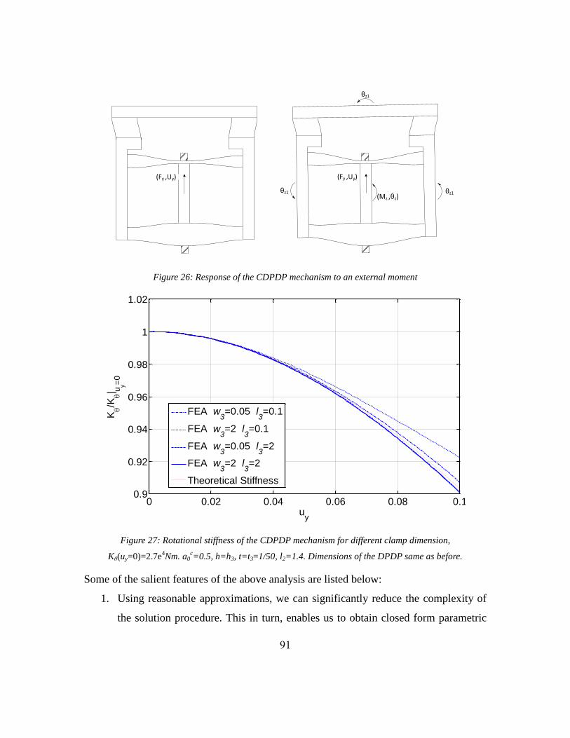
91
(Fy ,Uy) (Fy ,Uy)
(Mz ,θz)θz1 θz1
θz1
Figure 26: Response of the CDPDP mechanism to an external moment
Figure 27: Rotational stiffness of the CDPDP mechanism for different clamp dimension,
Kθ(uy=0)=2.7e4Nm. a0
c=0.5, h=h3, t=t3=1/50, l2=1.4. Dimensions of the DPDP same as before.
Some of the salient features of the above analysis are listed below:
1. Using reasonable approximations, we can significantly reduce the complexity of
the solution procedure. This in turn, enables us to obtain closed form parametric
0 0.02 0.04 0.06 0.08 0.10.9
0.92
0.94
0.96
0.98
1
1.02
uy
Kq/K
q| u
y=0
FEA w3=0.05 l
3=0.1
FEA w3=2 l
3=0.1
FEA w3=0.05 l
3=2
FEA w3=2 l
3=2
Theoretical Stiffness
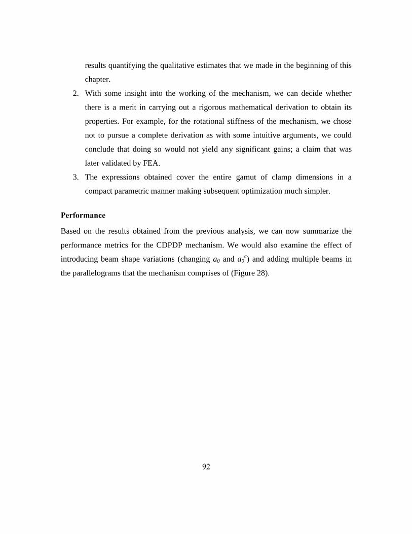
92
results quantifying the qualitative estimates that we made in the beginning of this
chapter.
2. With some insight into the working of the mechanism, we can decide whether
there is a merit in carrying out a rigorous mathematical derivation to obtain its
properties. For example, for the rotational stiffness of the mechanism, we chose
not to pursue a complete derivation as with some intuitive arguments, we could
conclude that doing so would not yield any significant gains; a claim that was
later validated by FEA.
3. The expressions obtained cover the entire gamut of clamp dimensions in a
compact parametric manner making subsequent optimization much simpler.
Performance
Based on the results obtained from the previous analysis, we can now summarize the
performance metrics for the CDPDP mechanism. We would also examine the effect of
introducing beam shape variations (changing a0 and a0c) and adding multiple beams in
the parallelograms that the mechanism comprises of (Figure 28).

93
2T3/Nc (L3,a
0c )
Clamp
PrimaryStage
GroundAnchor
GroundAnchor
Rigid Link
(Fy,Uy)
(Fx, Ux)
(Mz, θz)
Parallelogram 1 Parallelogram 2
(L,a0)
Nc
Beams
2T/N
NBeams
NBeams
Figure 28: CDPDP Mechanism with multiple grouped reinforced beam flexures. Normalization would still
be done w.r.t the original parameters (T and T3)
Range of motion
The range of motion of the mechanism would be the same as that of the DP and the
DPDP mechanisms given by equation (3.59). Moreover, the effect of adding multiple
beams or varying the degree of reinforcement a0 would also be the same as that shown in
Figure 17.
Error motions
Like in the case of the DPDP mechanism, due to symmetry, both the axial and rotational
error motions would be theoretically zero.

94
Motion Direction Stiffness
Figure 29: The motion direction stiffness of the CDPDP mechanism for different dimensions of the clamp.
The solid lines represent the predicted values whereas the circles show the corresponding FEA results.
w1=1.0, w2=0.8, l2=0.9, t=t3=1/50, h=h3
The motion direction stiffness in the absence of a bearing direction load is given by
equation (4.14). The predicted (equation (4.14)) and the FEA results8 for different clamp
dimensions have been found to be in good agreement (<5% error) as can be seen from
Figure 29. As expected, there is virtually no dependence on the dimensions W3 and L2.
For cases where stiffening is small, there is some discrepancy between the plots. This can
be attributed to motion direction stiffening in the DPDP mechanism which was not
captured in the BCM model. Because of the non-zero opposing theta error motions (3.60)
of each of the double parallelograms, internal moments get generated. Furthermore, due
to the weak dependence of the y direction force displacement relations of the double
parallelogram on the applied moment, these moments, in turn, cause stiffening.
8 The stiffness was calculated using the forward difference method i.e. Ky(i)=(Fy(i)- Fy(i-1))/(Uy(i)-Uy(i))
0 0.025 0.05 0.075 0.1 0.125 0.1524
26
28
30
32
34
36
38
40
42
uy
ky
w3=0.05 l
3=0.2
w3=0.05 l
3=0.2
w3=0.5 l
3=0.2
w3=0.5 l
3=0.2
w3=0.05 l
3=1.0
w3=0.05 l
3=1.0
w3=0.5 l
3=1.0
w3=0.5 l
3=1.0

95
For the multiple-beam configuration, equation (4.14) can be rewritten as:
0 1 2
11 0 11 02
320 1 3 3
11 0 11 02 3 3
3
4 32
2
4
y y
c
c
k k a k a uN
h tNk a k a
N ht l
(4.23)
The above equation shows that we can decrease the nominal stiffness of the mechanism
by increasing the number of beams (while simultaneously thinning them) in the
parallelograms of the base DPDP mechanism. However, if we wish to decrease the
relative amount of stiffening, we should increase the number of beams in the clamp
parallelograms in a manner such that Nc>N. Doing this would also reduce the lower
bound on the l3 which is evident from the updated version of equation (4.15):
1/32
0 123
211 0 11 03 3
3 3 0 max11 0
3.75
c
y
c
k a k ah tNl u
N ht k a
(4.24)
In a later section, we would see how this would increase the scope for making the clamp
more compact.
In the presence of a bearing load, which is much larger than the stiffening force fx1, this
stiffness is given as:
21
110
11 0 0
11 11
2 18 2
x
y
f kk k
k k
(4.25)
As discussed before, the clamp reduces the softening effect of the bearing force and in the
limiting case it is completely eliminated. In Figure 30 , we plot this stiffness for different
values of η (and γ) and compare it with FEA results. The Figure 30 shows that for small
to moderate values of η, the values match closely. However, for larger values where the
softening term is expected to decrease continuously with increasing η, the FEA results
show that this term saturates to a constant value.

96
Figure 30: Softening due to bearing direction loads in the motion direction. At large values of effectiveness,
there is a clear discrepancy between FEA and closed form results
This discrepancy can be eliminated if we include the second order terms in the expression
for the motion direction stiffness of a parallelogram i.e.:
2
0 1 2
11 11 1122
xy x y
ff k f k k u
(4.26)
Substituting this expression in the transverse direction relations in equation (4.16), and
thereafter rewriting equations (4.19):
1 2 120 11 11 11
11 11 0 0 0
11 11 11
1 2 120 11 11 11
22 11 0 0 0
11 11 11
1 14 16 2 2
1 14 16 2 2
x x xy y
x x xy y
f k f k f kf k u
k k k
f k f k f kf k u
k k k
(4.27)
Finally, using equations (4.17) and (4.27) we get:
2
12
110 21111 0 0
11 11
2 188 2
y x y
k kf k f u
k k
(4.28)
102
103
104
10-4
10-3
10-2
10-1
100
ky(f
x=0)-
ky(f
x=5)
FEA
Closed Form

97
Figure 31 shows the comparison between the stiffness given by the above equation and
the corresponding FEA results and shows good agreement between the two. Thus, for
large effectiveness, we still have a small softening term left over. Nevertheless, we can
still say that an effective clamp makes the motion direction stiffness fairly insensitive to
non-linearity arising due side loading which can simplify the design of controllers in the
case of comb drive actuators where errors in fabrication can lead to an offset between the
comb banks causing an unpredictable bearing force.
Figure 31: Softening in the motion direction due to bearing direction loads. Comparison between closed
form solution with second order correction and corresponding FEA results
With multiple beams, equation (4.25) becomes:
212 4
110
11 2
0 0
11 11
22 1
22 2
2
x
y
f kNk k
N Nk k
(4.29)
102
103
104
10-2
10-1
100
ky(f
x=0)-
ky(f
x=5)
FEA
Closed Form

98
The above expression is completely independent of Nc. Moreover, increasing N causes a
reduction in the nominal stiffness but increases the softening due to the applied force
significantly (proportional to N4 when the η=0 and N
2 as η becomes large).
Bearing Direction Stiffness
The bearing direction (x) stiffness can be obtained using equation (4.22):
212
112
11 033 11
1
21
2 8 2
x
y
k
kuk
k k
(4.30)
The bearing stiffness is plotted against FEA data for different values of the effectiveness
η in Figure 32. The plot shows that there is less than a 5% discrepancy between the
predicted and the FEA results which is acceptable for most applications. In our analysis,
we have not imposed any bounds on the effectiveness assuming that we can make it as
large as possible by just changing the dimensions of the clamp. However, this is not true
and the effectiveness is directly limited by the rotational stiffness of the double
parallelogram. Figure 33 shows the bearing stiffness for different values of effectiveness
for a smaller rotational stiffness of the double parallelogram (small w1 and w2). The error
increases at larger values of effectiveness which is probably because for these
dimensions, the rotational stiffness of the clamp becomes comparable to that of the
DPDP. This in turn causes the secondary stages to rotate with the clamp reducing the net
deflection of the clamp parallelograms which leads to lower moments Mz1,2, a lower
constraint force Fy1 and consequently lowers the effectiveness of the clamp. This effect
has been illustrated in Figure 34. This case has been dealt with in some detail in
Appendix C.

99
Figure 32: The bearing stiffness of the CDPDP mechanism for different values of effectiveness. The solid
lines represent the predicted values whereas the circles show the corresponding FEA results. w1=1.0,
w2=0.8, l2=0.9, t=t3=1/50, h=h3.
Figure 33: Bearing stiffness for w1=0.3, w2=0.2, l2=0.9, t=t3=1/50, h=h3.
0 0.025 0.05 0.075 0.1 0.125 0.150
1
2
3
4
5
6x 10
4
uy
kx
=463.891
=463.891
=46389.1
=46389.1
=92.7781
=92.7781
=9277.81
=9277.81
=0
0 0.025 0.05 0.075 0.1 0.125 0.150
1
2
3
4
5
6x 10
4
uy
kx
=463.891
=463.891
=46389.1
=46389.1
=92.7781
=92.7781
=9277.81
=9277.81
=0
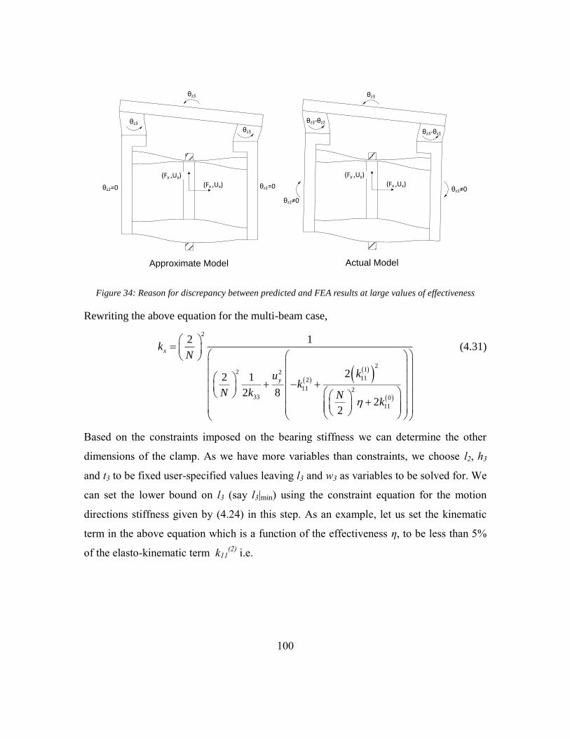
100
Actual Model
(Fy ,Uy)
(Fx ,Ux)θz1≠0
θz2≠0
θz3
θz3-θz2
θz3-θz1
Approximate Model
(Fy ,Uy)
(Fx ,Ux)θz2=0 θz1=0
θz3
θz3
θz3
Figure 34: Reason for discrepancy between predicted and FEA results at large values of effectiveness
Rewriting the above equation for the multi-beam case,
2
212 2
112
11 233 0
11
2 1
22 1
2 82
2
x
y
kN
kuk
N k Nk
(4.31)
Based on the constraints imposed on the bearing stiffness we can determine the other
dimensions of the clamp. As we have more variables than constraints, we choose l2, h3
and t3 to be fixed user-specified values leaving l3 and w3 as variables to be solved for. We
can set the lower bound on l3 (say l3|min) using the constraint equation for the motion
directions stiffness given by (4.24) in this step. As an example, let us set the kinematic
term in the above equation which is a function of the effectiveness η, to be less than 5%
of the elasto-kinematic term k11(2)
i.e.

101
21
11 2
112
0
11
212
11 0
112
11
20.05
22
4022
kk
Nk
kk
N k
(4.32)
Substituting the value of η from equation (4.11)
212 3 2
11 0 00 23 11 0 3 min2
3 3 11 0
4022 |
6
c k aa ht lw k a l
N h t k a
(4.33)
Using a value of l3=0.57 (for a motion direction stiffening of 5%) and assuming h=h3,
t=t3, l2=2, a0=a0c=0.5, N=2, T=1/200, l2=2, the required w3 comes out to be 0.44. As we
would see later, there is seldom a need for such conservative bounds on the bearing and
motion direction stiffness in which case, the overall clamp dimensions can be made
smaller. Moreover, by using multiple beams such that Nc>N, l3|min can be reduced
(equation (4.24)) and consequently the lower bound on w3 would decrease according to
equation (4.33). Finally, the degrees of reinforcement a0 and a0c can be changed to further
alter the bounds on l3 and w3. The choice of a0 and N would be made based on the
application requirements as they primarily dictate the motion and the bearing direction
stiffness of the mechanism (assuming that the clamp is effective). Beyond this point,
using equations (4.24) and (4.33), we can choose a0c and Nc to obtain the smallest
possible size of the clamp.
0.1
0.20.3
0.40.5 2
46
810
0.2
0.4
0.6
0.8
1
Nca
0
c
l3| m
in
0.10.2
0.30.4
0.5 24
68
10
0.1
0.2
0.3
0.4
0.5
Nca
0
c
w3| m
in

102
Figure 35: l3|min and w3|min for different clamp variations
As an example, let us assume a0=0.5 and N=2. Figure 35 shows l3|min and w3|min for
different values of Nc and a0c. From the plots, we can infer that a large value of Nc would
be preferred. However, this is not always possible as the minimum thickness and hence
the largest possible Nc is often limited by manufacturing capabilities. Increasing a0c
decreases l3|min but increases w3|min. However, we notice that:
0 0
3 min 3 min
0 0
| |
c c c c
c c
N N N N
w l
a a
(4.34)
i.e. the rate of increase of w3|min with increasing a0c is larger compared to the rate of
increase in l3|min with decreasing a0c which implies that the optimum point would be close
to a0c=0.1. The exact optimization would depend on the relative weights assigned to the
two dimensions. For example, if the footprint is not sensitive to small variations in w3|min,
the optimization can be solely done to minimize l3 (i.e. a0c→0.5 and large Nc).
The rotational stiffness, as we discussed before, would remain relatively unchanged and
hence, would exhibit the same trends as those seen in Figure 17.
THE DOUBLE PARALLELOGRAM – TILTED-BEAM DOUBLE PARALLELOGRAM (DP-
DTB)
The DP-DTB mechanism shown in Figure 36 offers an improved bearing stiffness
compared to the DPDP mechanism without using any additional topological features like
in the Lever-DPDP and Clamped-DPDP mechanisms. This mechanism has been
presented and discussed previously [24, 36, 43] and a summary is presented here. The
improved bearing stiffness of this mechanism is due to the complementary behavior of
the DP and the TDP flexures. Referring to Figure 37, if the primary stage of a TDP
mechanism is not rotationally constrained, the secondary stage is free to move in the y
direction when a y displacement is applied at the primary stage. This unconstrained

103
motion of the secondary stage, in a manner similar to that in the DP-DP mechanism,
causes a bearing stiffness drop in the TDP mechanism as well. However, when a θ
constraint is applied at the primary stage along with a specified y location, two
conflicting instantaneous centers of rotation C1 and C2 are created for the secondary
stage locking its motion. (This affect does not occur in a DP flexure as in that case C1
and C2 are at infinity). The DP flexure with its superior rotational stiffness, provides this
constraint and hence stiffens the TDP flexure in the bearing direction subsequently
improving the bearing stiffness of the entire mechanism. Furthermore, unlike the DP-DP
flexure, the decline in the stiffness ratio in this case is dictated by the weak
elastokinematic effect, which can be further reduced via beam shape optimization (degree
of reinforcement a0).
(Fy,Uy)
(Fx, Ux)
(Mz, θz)
Ground
Anchor
Ground
Anchor
β
α
2W2 2W1
(L ,a0) (L,a0)
Secondary
Stage
Secondary
Stage
Primary
Stage
Figure 36: The Double Parallelogram- Tilted Beam Double Paralleogram (DP-TDP)

104
β
α
(Mz, θz=0) C1 C2
Figure 37: Constraint behavior of the TDP flexure
The analysis for the TDP flexure has been done by awtar et.al. [24]. However, due to the
asymmetric nature of the overall DP-TDP mechanism, obtaining a closed form analytical
solution is difficult, if not impossible. Another problem is the large internal forces and
moments that get generated between the two halves of the mechanism. For such large
forces, the approximate BCM model might no longer be valid and hence, the solution that
we obtain using the model could be fairly inaccurate. Hence, we resort to using extensive
FEA analysis to qualitatively discuss some characteristics of this mechanism. Table 5
shows the parameters used for the non-linear FEA. The tilt angles α and β were chosen as
the variables for this analysis as they have the strongest influence on the characteristics of
the mechanism.
Table 5: Dimensions of the DP-TDP flexure used in the FEA analysis.
Dimension Value (microns)
L 1000
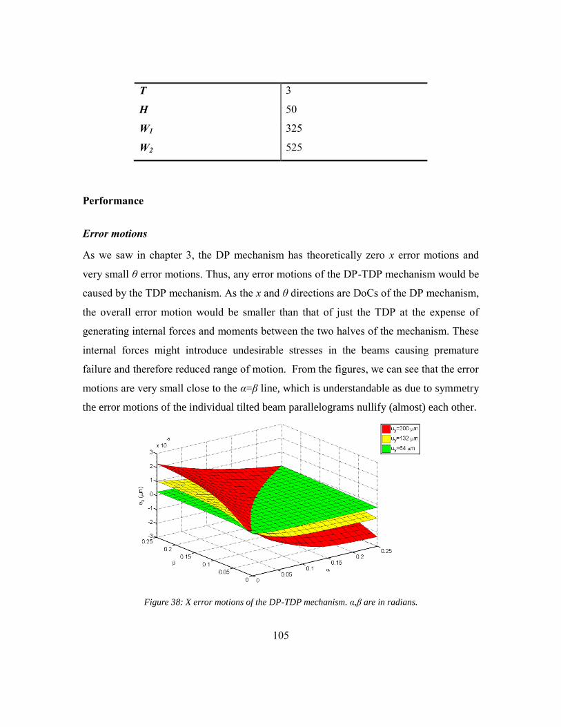
105
T 3
H 50
W1 325
W2 525
Performance
Error motions
As we saw in chapter 3, the DP mechanism has theoretically zero x error motions and
very small θ error motions. Thus, any error motions of the DP-TDP mechanism would be
caused by the TDP mechanism. As the x and θ directions are DoCs of the DP mechanism,
the overall error motion would be smaller than that of just the TDP at the expense of
generating internal forces and moments between the two halves of the mechanism. These
internal forces might introduce undesirable stresses in the beams causing premature
failure and therefore reduced range of motion. From the figures, we can see that the error
motions are very small close to the α=β line, which is understandable as due to symmetry
the error motions of the individual tilted beam parallelograms nullify (almost) each other.
Figure 38: X error motions of the DP-TDP mechanism. α,β are in radians.

106
Figure 39: Theta error motions of the DP-TDP mechanism
Motion Direction Stiffness
The tilted configuration of the beams in the TDP flexure causes an increase in the
nominal motion direction stiffness of the mechanism. For every tilted beam parallelogram
in the TDP flexure, the y direction stiffness is directly proportional to the secant of the tilt
in the beams. But as the tilt angles are small, the increase in stiffness is not significant. In
the DP-TDP flexure, the primary cause for motion direction stiffening is the internal
bearing direction forces and moments brought about by the kinematic conflict between
the error motions of the DP (theoretically zero) and the TDP flexure. It is because of
similar reasons that the P-P flexure has a Ky which increases exponentially with y
displacements which makes it a poor single axis bearing even though it has a satisfactory
bearing stiffness Kx. Therefore, the trends seen in Ky of the mechanism is similar to those
seen in the error motions and as before, the tilt angles close to the α=β line would be
optimal.

107
Figure 40: Motion direction stiffness of the DP-TDP flexure
Bearing Direction Stiffness
For the TDP flexure, in the limiting case as α,β→0 i.e. as it approaches the DP flexure,
the instantaneous centers of rotation tend to infinity and hence, no longer oppose each
other allowing unconstrained y motion of the secondary stage. As these angles increase in
magnitude, the kinematic constraint on the secondary stage also increases. Figure 41
shows that for tilt angles greater than 0, we see an improvement in the x direction
stiffness which gradually increases as either or both of them increase and saturates at a
certain angle (where the elasto-kinematic effect starts dominating the stiffness drop).
Beyond this point, the trend reverses and we see a small decline in the stiffness because
of the effect of the reduced nominal stiffness due to the tilt of the beams. The analysis
also shows that the bearing stiffness depends on the magnitude and direction of the axial
force and moment. However, they don’t change the trends seen in the plots and therefore,
for the purpose of this qualitative discussion, we would ignore this dependence.

108
Figure 41: X direction stiffness of the DP-TDP flexure
Figure 42: θ Direction Stiffness of the DP-TDP mechanism
The rotational stiffness falls significantly for α,β>0. In fact Kθ for the DP-TDP
mechanism is almost half that of the DP-DP mechanism. This is understandable as the
rotational stiffness of the TDP flexure is much smaller than that of the DP flexure due to
the presence of instantaneous centers of rotation C1 and C2. Figure 42 shows that tilt
angles such that α≤β would be preferred.
Considering all the characteristics discussed so far in conjunction, almost equal tilt angles
α,β less than 0.15 radians would yield the most desirable properties of the DP-TDP

109
flexure. In chapter 6, we would use these results to conduct a case specific optimization
using the objective function given by equation (1.18).
In the next chapter, we would discuss the direct experimental validation for the results
obtained for the CDPDP mechanism using a macro-scale modular, low cost and high
precision setup. In a subsequent chapter, we would also briefly touch upon the indirect
measurement of these attributes using micro-scale comb drive actuators.

110
Chapter 5: Experimental Validation of the Clamped Paired Double
Parallelogram (CDPDP) mechanism
Closed form parametric results for the stiffness and error motions were obtained in the
last chapter for the CDPDP mechanism which were validated using FEA analysis. In this
chapter, we would further validate these results by directly measuring forces and
displacements at the primary stage in a macro-scale experimental setup. The experiment
was designed to be reconfigurable so as to accommodate some variations of the
mechanism without redesigning the entire setup. Moreover, as cost was a constraint,
some novel low-cost methods were used for load application and measurement without
compromising the precision of the results.
Measurement Scheme
An obvious question is where should we apply the loads and measure the resultant
displacements? In all our previous analysis, the point of application of the loads was
arbitrarily chosen to be at the center of the primary stage. However, if this location does
not exactly coincide with the location of the center of stiffness of the mechanism, there
would be a moment that would be generated in addition to the force causing a small
rotation. This moment doesn’t affect the bearing or motion direction stiffness of the
mechanism because of the decoupling between the x, y and the θ direction force
displacement relations.
P
C
Primary Stage
(Fx,UxC)
(Fy,UyC)
(FxLPC+FyWPC,θzC)
P
C
(Fx,UxP)
Primary Stage
(Fy,UyP)
LPC
Wpc
≡
Figure 43: Center of stiffness of the mechanism

111
In the experimental setup, however, the x (or y) displacement measured at any point
would comprise of the pure x (or y) displacement brought about by the application of the
load fx (or fy) and the rotation due to the moment applied about the COS (Figure 43) i.e.:
xP xC PC CU U L q (5.1)
As the stiffness is defined w.r.t. displacement and forces at the COS of the mechanism,
we need to decouple the two components of the x displacement. For doing this, we need
to know the location of the COS. Although the location of the COS, which is a function
of the y displacement in most cases, can be determined using the BCM model and finite
element analysis, its exact location in the actual setup might differ significantly due to
manufacturing imperfections. It is because of the same reasons that we cannot apply
loads and measure displacements at the COS directly. Thus, we would need a method to
determine the COS experimentally as well. The derivation of the COS for the CDPDP
mechanism has been done in the Appendix D. It was observed that the COS has a very
weak dependence on the magnitude of the force fx but depends on the displacement uy.
Hence, for the experimental validation, we can assume the COS to be a function of uy
only.
The objective of the experiment would be to obtain the following characteristics of the
mechanism:
1. Location of the center of stiffness at every y displacement (C)
2. Error motions (ex(uy), eθ(uy))
3. Motion direction stiffness (ky)
4. Bearing direction stiffness (kx, kθ)
The last three properties have to be found w.r.t. the COS of the mechanism. The above
objectives translate to the following:
Apply
112
1. A motion direction displacement Uy
2. An x-direction force which maintains perpendicularity with the motion direction
at all displacements
3. A moment on the primary stage
Measure
1. Motion direction load Fy at every Uy
2. X-displacement of the primary stage
3. Rotation of the primary stage
Due to symmetry of the mechanism about the axis parallel to the y-axis and passing
through the center of the primary stage, we can assume that the x-location of the COS is
close to this axis. Hence, we can decouple the measurement of the Y-direction stiffness
from x and θ direction measurements. Thus, using a force sensor to measure Fy and a
displacement sensor to measure Uy, we can find the motion direction stiffness of the
mechanism. For this, we could use the forward difference approach:
y yf y yi
y yi
yf yi
F U F UK U
U U
(5.2)
Where (Uyf-Uyi) is small. Or instead, we could obtain a polynomial curve-fit for the data
points – (Fy, Uy) and use the slope of the curve to obtain the motion direction stiffness.

113
S1
S2
S
C
DUs1
Us2
X
Y
Z
Figure 44: The placement of the sensors for measuring x-direction displacements and rotations of the
stage.
For obtaining the rest of the properties, we use two displacement sensors for the primary
stage which would measure rotation as well as the x direction displacement of the stage.
For now, let us assume that these sensors labeled S1 and S2 are placed a distance D
(unknown) from the C with a separation of S (known) between each other as shown in the
Figure 44. The sensors measure displacements Us1 and Us2 in the x-direction. From these
two readings, we can obtain the rotation and the x displacement at the COS:
2 1
12
S S
zC
xC s
U U
SS
U U D
q
q
(5.3)
The error motions can be obtained in terms of D by actuating the motion stage in the Y
direction with no bearing loads acting on it i.e.:
2 1
1
| |
|2
s No Load s No Load
y
x y s No Load y
U UE U
SS
E U U D E U
q
q
(5.4)
We now have three unknowns D(Uy), Kx(Uy) and Kθ(Uy) left to determine. For this we use
a scheme where we apply two forces at different y locations of the primary stage
individually at every y displacement as shown in Figure 45.

114
Fx1
S1
S2
S
C
D
ΔUs11
Δ Us21
R1
Configuration 1 Configuration 2
S1
S2
S
C
D
ΔUs12
Δ Us22
R2
Fx2
Primary Stage
Figure 45: Force application on the primary stage. Also, ΔUs11= Us1|load=Fx1- Us1|no-load.
Using this we get two separate sets of sensor displacements for every force applied. For
every force we can write out four equations as follows:
21 11 22 12
1 2
1 1 2 21 1 1 2 2 2
1 2
1 11 1 2 12 2
11 1 1 2 2 2
1
, , , ,
2 2
, , , ,
s s s s
z y z y
x xy x x y y x x y
z y z y
x y s z y x y s z y
xx y x x x y x y x x x y
x y
U U U UU U
S SF R F R
K U F F R K U K U F F R K UU U
S SU U U D U U U U D U
FK U F F R K U K U F F R K U
U U
q q q q
q q
q q
q q
2
2
x
x y
F
U U
(5.5)
Moreover, the y separation between the two forces can be known beforehand giving:
1 2sepR R R (5.6)
If we take into account all the dependencies of the x and θ stiffness expressions on the
magnitude of the forces and moments applied, we have an under-determined system with
10 unknowns and 9 equations implying that we need to know the exact location of the
COS to begin with in order to calculate the x and θ stiffness. However, if we ignore these
dependencies in the rotational stiffness, we can determine all the unknowns in the
equations at every y displacement uy.

115
Design of the setup
The first task was to choose the dimensions of the mechanism. As there wasn’t a
particular application that had to be designed for, the mechanism was designed around
the available sensors, actuators and manufacturing capabilities. These are listed below:
Actuation
Motion (Y) Direction
The motion direction has to be actuated using a position actuator. For this purpose, a PI
actuator M-227.25 [55] with a lead-screw driven by a closed loop DC motor (Figure 46)
was used. It has a stroke of 25 mm, can provide a maximum push/pull force of 40N and
can withstand a maximum lateral force of 0.1N. Moreover, it also houses the rotary
encoder with a minimum incremental motion of 0.05 μm. Finally, the actuator has a
backlash of 2 μm. The actuator thus imposes the following constraints on the mechanism:
max
max
max
| 40
| 0.1
12.5 | 12.5
2
y
x actuator
y
y
F N
F N
mm U mm
U m
(5.7)
X (Bearing Direction)
Y (Motion Direction)
Flexure Clamp
CouplingBlock
ActuatorIsolator
DC-Mic CDPDPMechanism
Figure 46: The DC-mic assembly

116
The DC-mic is held in place by a flexure clamp as shown in Figure 46 to apply an even
distributed clamping force on the body of the actuator. To prevent damage on the DC-mic
due to lateral forces, an actuator isolator between the mechanism and the actuator is
necessary. In this case it is simply a beam with high stiffness in the y direction but large
compliance in the x direction which helps absorb parasitic displacements in that direction.
Bearing (X) direction
A side load has to be applied on the motion stage at two different locations for different
uy. This loading has to maintain perpendicularity with the motion direction at all y
displacements. For this purpose a novel scheme was utilized.
Firstly, instead of using a pulley and weights suspension to apply the side load where
because of friction, total load transmission might not occur, a virtual pulley in the form of
a three string junction was used for load transmission as shown in Figure 47. By choosing
the angle between the strings, we can control the amount of load applied on the stage:
cot cotx LF F W (5.8)
W
φ
FL
Fx
Primary stage
XX (Bearing Direction)
Y (Motion Direction)
Fx
Alignmentpins

117
Figure 47: Three-string junction for load transmission to the primary stage of the mechanism
Moreover, as we know that for typical millimeter-scale dimensions, the x-direction
motion would be of the order of a few microns9, we can assume that the angle between
the strings wouldn’t change significantly when the weights are suspended thereby
avoiding the need for readjusting the angle every time after applying the load or
displacing the stage in the y direction. A protractor can be used to measure the angles to
within a degree. We would later see that this uncertainty wouldn’t significantly affect the
accuracy of the measurements.
In order to maintain perpendicularity, an alignment plate was used with embedded
dowels pins. The pivot of the string setup is on a stand resting on a manual xy stage (Thor
Labs MT1) which has a range of 0.5” in each direction. Thus, whenever the primary stage
is displaced, the manual stage can also be displaced along with the suspended weight to
ensure marginal contact with the outer dowel. This scheme imposes the following
restriction on the mechanism:
max6.35 | 6.35ymm U mm (5.9)
X (Bearing Direction)Y (Motion
Direction)
Primary Stage X
Y
W
Fx
Manual Stage
Alignment Plate
Alignment Pin
Figure 48: Top view of the three string junction. The manual stage can be moved in the y direction to keep
marginal contact with the alignment pin.
9 Later, after all the dimensions are selected, this condition would be checked again to ensure that it is still
satisfied.

118
Sensing
Motion (Y) direction force Fy
A load cell (ELFS- T3E-20L) [56] was sandwiched between the DC-mic and the
mechanism to measure the force Fy as shown in Figure 49. The range of the load cell was
20 Lb, much higher than the maximum load that the DC-mic can withstand. As the
experiment was essentially a quasi-static one, the noise in the measurement could be
minimized significantly by using strong low-pass filters and/or long sampling windows.
DC-Mic
Adapter
LoadCell
AdapterAdapter
Split-RingSleeve
Couplingblock
Figure 49: Integration of the load-cell in the DC-mic assembly
Bearing direction displacements (Ux and θz)
Two capacitive probes (C23-C Low Resolution [57]) in a configuration shown in Figure
44 are used for measuring these displacements. These are implemented in the setup as
shown in Figure 50. These are ideally suited for this application as they are tolerant to
relatively large Y displacements perpendicular to their measurement axis and have a small
range (50 microns) with a high achievable resolution (~10nm).
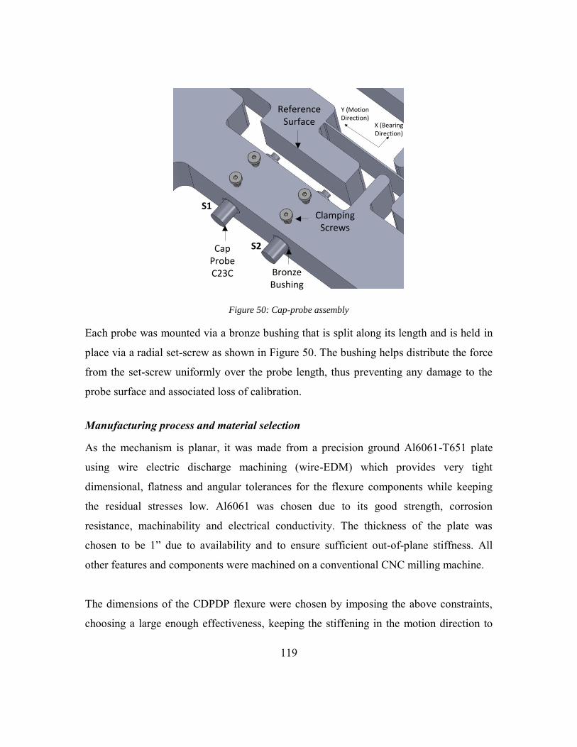
119
S1
S2CapProbeC23C Bronze
Bushing
ClampingScrews
ReferenceSurface X (Bearing
Direction)
Y (Motion Direction)
Figure 50: Cap-probe assembly
Each probe was mounted via a bronze bushing that is split along its length and is held in
place via a radial set-screw as shown in Figure 50. The bushing helps distribute the force
from the set-screw uniformly over the probe length, thus preventing any damage to the
probe surface and associated loss of calibration.
Manufacturing process and material selection
As the mechanism is planar, it was made from a precision ground Al6061-T651 plate
using wire electric discharge machining (wire-EDM) which provides very tight
dimensional, flatness and angular tolerances for the flexure components while keeping
the residual stresses low. Al6061 was chosen due to its good strength, corrosion
resistance, machinability and electrical conductivity. The thickness of the plate was
chosen to be 1” due to availability and to ensure sufficient out-of-plane stiffness. All
other features and components were machined on a conventional CNC milling machine.
The dimensions of the CDPDP flexure were chosen by imposing the above constraints,
choosing a large enough effectiveness, keeping the stiffening in the motion direction to

120
be less than 5% and maintaining an adequate safety margin against yielding, and have
been tabulated in Table 6 along with their justifications. The CDPDP flexure plate is also
shown in Figure 51. The clamp has been moved inside the outer parallelogram to make
the mechanism more compact.
Table 6: Dimensions of the CDPDP mechanism
Dimension Value Justification
L 65mm
Keeping the maximum
displacement around 0.1L to
maintain adequate safety
margin against yielding of
the beams.
T 0.8mm
To ensure that the
maximum motion direction
force is less than 40N
a0 0.3
Optimum value: Improves
bearing stiffness
considerably while not
significantly increasing the
y-direction stiffness
H 25.4 mm Standard thickness of the
plate
W1 70.52mm Rotational stiffness of the
DPDP unit >> rotational
stiffness of the clamp W2 24.14mm
W3 32.5mm Large clamp effectiveness
L2 90.5mm
L3 32.5mm Low stiffening in motion
direction and large

121
effectiveness
LT
L3 X (Bearing Direction)
Y (Motion Direction) 2W3
a0L
2W2
2L2
2W1
Figure 51: The CDPDP flexure plate
Design of Auxiliary Components and Dimensions
Actuator Isolator
The actuator isolator shown in Figure 52, i.e. a single beam positioned along the motion
direction y, must be significantly more compliant in the x direction compared to the
CDPDP mechanism. Therefore, its dimensions were chosen such that the stiffness of the
isolator is almost four orders of magnitude smaller than the lowest x-direction stiffness of
CDPDP mechanism i.e.
4106
x Isolator
x CDPDP y
k
k U mm
(5.10)

122
Using equation (4.30) for the bearing stiffness of the CDPDP mechanism with the
dimensions given in Table 6 and the motion direction stiffness of a single beam given by
equation (2.11), the length Li of the actuator isolator was chosen to be 50mm (the beam
cross-section was chosen to be the same as that in the CDPDP mechanism).
Li
T
X (Bearing Direction) Y (Motion
Direction)
Figure 52: The actuator isolator with dimension labels
Separation between cap-probes (D) and points of load application (Rsep)
The sensor and actuation arrangement for the bearing stiffness measurement shown in
Figure 45 is implemented on the flexure plate as shown in Figure 53. Table 7 shows the
values of the dimensions involved.
S1S2
S
12
Fx1Fx2
RsepD*X
COS
R2 R1
Figure 53: Implementation of the measurement scheme shown in Figure 45. D*=D-R2-S/2

123
Table 7: Parameters of the measurement scheme
Dimension Value
S 30mm
Rsep 43mm
D* 103mm
Fillets at flexure ends
In the absence of fillets at the ends, the stiffness of the flexure beams can be significantly
smaller than that predicted by closed form and FEA analysis which assume the support to
be perfectly rigid. This is due to additional local flexibility at the juncture of a support
and a flexure beam. Moreover, sharp corners can lead to large stress concentrations
thereby causing premature static or fatigue failure of the mechanism. Howell et.al. [58]
have analyzed this configuration and have obtained optimal fillet radii to mitigate these
effects given below:
0.64 For half-plane junctures
1.1 For quarter-plane junctures
fillet
fillet
R T
R T
(5.11)
These fillet radii have been used in all flexure-support junctions (Figure 54) in the
mechanism.

124
R=1.1T R=0.64T
T T
Quarter Plane
Half Plane
Figure 54: Fillets at flexure supports
Thickness of ‘rigid’ sections and stages
In all the previous analysis, all the stages were assumed to be perfectly rigid. In order to
ensure this, the thickness of the stages was chosen to be such that the bending stiffness is
almost three orders of magnitude larger than the flexure bending stiffness. As exact
expressions are cumbersome to derive and an overkill for this purpose, we simply use the
fact that the bending stiffness is proportional to (T/L)3. Comparing the bending stiffness
between the stages and flexure strips and setting the ratio between them at O(103), a
minimum stage thickness of 14mm was obtained (Figure 55).
For the sections between flexure strips, an order of magnitude difference was set between
bending stiffness ratio for the compliant and rigid sections leading to a thickness value of
3T for the rigid sections.

125
TS=14mmT=0.8mm TR=2.4mm
Figure 55: Thickness of rigid sections and stages
Finally, Figure 56 shows the entire setup with all the components labeled including the
load-cell and cap-probe amplifiers and the DC-mic driver along with the USB data-
acquisition board connected to a host computer (not shown). The entire setup rests on a
vibration isolation table to minimize effects of floor vibration (moreover, as mentioned
before, long sampling windows are also used to further minimize the effects of
extraneous noise and vibrations).

126
1
2
3
4
5
678
9
10
11
121413
Figure 56:Complete Experimental Setup - 1)Dc-Mic, 2) Flexure Clamp, 3)Load Cell, 4)Actuator Isolator,
5)Cap-probes, 6)CDPDP mechanism, 7) DC-Mic amplifier, 8)Cap-probe amplifier, 9)NI USB-DAQ,
10)Alignment plate, 11)String for applying load, 12)Alignment pins, 13)Suspended Weight, 14) Manual
stage and post
,
Error Analysis
The primary sources of measurement error/uncertainty in this experiment are the
following:
1. Cap-Probe Resolution – δUs (m)

127
2. Load-cell Resolution – δFy (N)
3. DC-Mic Encoder Resolution – δUy (m)
4. String Angle Resolution – δφ (rad)
All other angle misalignment errors – between the cap-probes and the reference surface
Figure 50 and between the bearing load (Fx) transmitting string and the horizontal/ground
Figure 47 or motion direction y Figure 48 can be ignored as they would vary as cosines of
the error and hence, would be small. Errors in the elastic modulus of the material can be
assumed to be less than 5% [59].
Errors in Motion direction stiffness
The motion direction stiffness is given by equation (5.2). Taking the variation on both
sides:
2
2 2
yf yi y yf y yi yf yi y yf y yi
y
yf yi
y y y
y yf yi y yf y yi
U U F U F U U U F U F UK
U U
K U F
K U U F U F U
(5.12)
Errors in bearing direction stiffness (Kx and Kθ)
Referring to Figure 45, the displacement measured by any particular cap-probe ΔUij
where i indicates the probe number and j corresponds to the pin on which the load fx is
applied is given by:
0| |
xjij ij load f ij loadU U U (5.13)
The error can be obtained by taking variation on both sides:

128
0| |
2
xjij ij load f ij load
ij s s s
U U U
U U U U
(5.14)
Using equation (5.5), the error in the measurement of the rotation θzj can be obtained:
2 1
4s j s j s
zj
U U U
S S
q
(5.15)
Similarly, the uncertainty in the applied loads Fxj due to errors in measurement of the
angle φ can also be calculated using equation (5.8):
2cot
sin
2
sin 2
xj j j j
j
xj
xj j
F W W
F
F
(5.16)
Using equations (5.5) and (5.6), the rotational stiffness can be solved for:
1 2
2 1 1 2
sep x x
y
x z x z
R F FK U
F Fq
q q
(5.17)
Taking the variation of the above on both sides:
1 2 1 2 1 1 21 2
1 2 2 1 1 2
x x z z x z xx x
x x x z x z
F F F FK F F
K F F F F
q
q
q q q
q q
(5.18)
Where errors in Fx and θz are given by equations (5.16) and (5.15) respectively. The
location of the center of stiffness is given by:
22
2
z
x
KR
F
qq (5.19)
Again, taking the variation of the above equation:
22 2
2 2 2
xz
z x
K FR
R K F
q
q
q
q (5.20)
Next, the error in the axial displacement can be calculated using equation (5.5):
1 11 2 1 1 2
2 1 1 2
* *
2 *x y s z z
s z z
U U U D R D R
U R D R
q q
q q
(5.21)

129
Finally, the uncertainty in the x-direction stiffness can be given by:
1 1
1 1
x x x
x x x
K F U
K F U
(5.22)
Uncertainty in parasitic motions (Ex and Eθ)
The parasitic motions are given by equation (5.4). Following a procedure similar to one
shown above, the estimates of uncertainty in these measurements are given below:
2 2
2
*
sy
x y s y y
UE U
SE U U D R E U E U R
q
q q
(5.23)
FEA Validation and predicted results
S1
S2
1
2
Fx1
Fx2
X
Y
Θ
Figure 57: Sign conventions used for the experiment

130
The experimental setup and procedure was simulated using FEA and the predicted
stiffness and displacement estimates were obtained. Figure shows the sign conventions
adopted for this experiment. As before, BEAM 4 elements were used to model the
compliant flexures and a force convergence tolerance of 10-3
was used. Figures Figure 58
to Figure 61 show the motion, rotational, axial stiffness and the distance R2 of the COS
from Pin 2 (Figure 53) calculated using FEA (solid lines) and closed-form results
(circles) for the mechanism with dimensions tabulated in Table 6. Error bars have also
been added using expressions derived in the last section. The values for measurement
uncertainties: δUs, δFy, δUy and δφ were chosen to be 5nm, 0.01N, 5 μm and 1 deg
respectively. Moreover, Fx1=Fx2=40N and φ1= φ2=0.25π Rad.
Figure 58: Motion direction stiffness for the CDPDP flexure plate
0 1 2 3 4 5
x 10-3
6600
6800
7000
7200
7400
7600
Uy (m)
Ky (
N/m
)
FEA
Closed Form

131
Figure 59: X direction stiffness for the CDPDP flexure plate
Figure 60: Rotational stiffness for the CDPDP flexure plate
0 1 2 3 4 5
x 10-3
5
5.5
6
6.5
7
7.5x 10
7
Uy (m)
Kx (
N/m
)
FEA
Closed Form
0 1 2 3 4 5
x 10-3
5.5
6
6.5
7
7.5
8
8.5
9
9.5x 10
4
Uy (m)
Kq (
Nm
)
FEA
Closed Form

132
Figure 61: Location of the COS for the CDPDP flexure plate. The closed form expressions are given by
equation (D.10)
Significant discrepancy can be seen between the FEA results and closed form results for
the X-direction stiffness shown in Figure 59. This can be explained by taking into account
the coupling between the x and θ direction relations. This case has been dealt with in
Appendix D and this error has been eliminated to some degree. Finally, the expected
displacements at the cap-probes and the rotations θz1 and θz2 have also been plotted in
Figure 62 and Figure 63.
0 1 2 3 4 5
x 10-3
3
4
5
6
7
8
9
10
11
12x 10
-3
Uy (m)
R2 (
m)
FEA
Closed Form

133
Figure 62: The expected displacement at the first cap-probe (S1) for loading on pin 1 and pin 2.
Figure 63: The expected rotations of the stage for loading on pin 1 and pin 2.Rotations are in radians.
0 1 2 3 4 5
x 10-3
-1.5
-1
-0.5
0
0.5
1
1.5
2x 10
-6
Uy (m)
U
s1
j (m
)
Us12
(FEA)
Us11
(FEA)
0 1 2 3 4 5
x 10-3
-0.5
0
0.5
1
1.5
2
2.5x 10
-5
Uy (m)
qz
qz1
(FEA)
qz2
(FEA)

134
Preliminary Results
Motion Direction Stiffness
The motion direction force vs. displacement curve is shown in Figure 64. The force was
observed to be predominantly linear with non-linearity of less than 3% over the range of
5mm. Thus, the clamp has negligible influence on the motion direction stiffness which is
desirable.
Figure 64: Experimentally measured motion direction force vs. displacement curve
0 0.5 1 1.5 2 2.5 3 3.5 4 4.5 5
x 10-3
-0.5
0
0.5
Uy (m)
F
y (
N)
Residuals
Cubic: norm of residuals = 0.18721
0 0.5 1 1.5 2 2.5 3 3.5 4 4.5 5
x 10-3
-20
0
20
40
60
Uy (m)
Fy (
N)
F
y = - 8.5186e+05*U
y
3 + 30301*U
y
2 + 6828.9*U
y - 0.031677
Experimental Data
Cubic Fit

135
Chapter 6: Case Study: Comb drive optimization
The comb drive actuator is an example of a single axis system whose performance is
directly affected by the quality of the flexure bearing. In this chapter, we use the results
obtained in chapter 4 to design comb drive actuators employing the CDPDP and DP-TDP
flexures as motion guides with the objectives of achieving the largest possible stroke with
minimum possible actuator effort and footprint. A systematic procedure to design comb
drive actuators with these attributes which are desirable in micro and nano-positioners
[60, 61] and micro-grippers [62, 63], would also be developed which can be used for
other flexure guides as well. This procedure also encompasses restrictions imposed by
fabrication capabilities and system requirements.
Uypr
(Fy=0 ,Uy=0)
(B) Pre-Bend=Uypr
(Fy=0 ,Uy=0)
(A) Pre-Bend=0
Figure 65: Pre-Bending in a DPDP flexure
-0.2 0 0.2u
y
-0.2 0 0.2u
y
-0.2 0 0.2u
y
(A) Pre-Bend=0 (B) Pre-Bend<Critical (C) Pre-Bend>Critical
-0.2 0.20uy
-0.2 0.20uy
-0.2 0.20uy
Kx/KyRequired Stiffness
Stroke Stroke Stroke
Figure 66: Effect of pre-bending on the stroke of a comb drive actuator. At the critical pre-bend, the
stiffness ratio curve intersects the required stiffness curve at exactly 3 points.

136
We would include certain design variations of the flexures – reinforced beams (Figure 7)
and pre-bending or pre-tilting [37, 64] (Figure 65) to further boost the performance of the
devices. Although the multi-beam parallelogram (Figure 12) can easily be incorporated in
the design process, it has been excluded from this analysis as it offers no obvious
advantage for this particular application. By pre-bending beams in a particular direction,
one can shift the stiffness profile of the flexure thereby delaying the onset of snap-in and
consequently increasing the stroke. This is illustrated in Figure 66 (B). However, there
exists a limit beyond which additional pre-bending can cause a pre-mature intersection
with the required stiffness curve (Figure 66 (C)). Thus, in order to maintain an adequate
safety margin to disturbances and manufacturing imperfections, the actual pre-bend is
kept sufficiently below this limit which can be easily determined for a flexure mechanism
based on its stiffness properties.
There are some fundamental differences between the optimization procedures for the
CDPDP and DP-TDP cases. The CDPDP mechanism has theoretically zero error motions
whereas the DP-TDP could have non-zero error motions (depending on the tilt angles).
Moreover, because of asymmetry, the sensitivity to fabrication imperfections would be
larger in the case of the DP-TDP mechanism which in turn would imply that the safety
margin given by equation (1.15) must be larger for this flexure. For the CDPDP
mechanism, we can simply use the snap-in condition given by equation (1.7) along with
the closed form stiffness expressions derived in chapter 4. Moreover, as its rotational
stiffness can be increased independent of the axial stiffness by increasing the beam
separations w1 and w2, we can further assume a purely one dimensional snap-in model
given by equation (1.6) instead of the two dimensional one (equation (1.7)) and choose
the separations to ensure that the difference in strokes predicted by (1.7) and (1.6) is
negligible. Consequently, for the optimization of the CDPDP mechanism for a comb
drive actuator, we can directly use the objective function given in equation (1.18). Such a
simplified governing equation for snap-in and hence a closed form objective function for
optimization does not exist for the DP-TDP case. Moreover, we do not have complete

137
parametric results for the stiffness and error motions of this mechanism yet. Therefore,
we would merely do a first-pass qualitative optimization for the DP-TDP mechanism here
and lay out some guidelines for future work.
CDPDP optimization
In this section, we present a systematic procedure for holistically designing a CDPDP
flexure based comb-drive actuator to maximize its actuation stroke while minimizing
device foot-print and actuation voltage. Given the several constraints and tradeoffs
involved, the goal here is to obtain a good starting point for the flexure and comb-drive
dimensions shown in Figure 23 and Figure 3 respectively (L, T, a0, W1, W2, L2, L3, W3, G,
Lf, and Tf ) based on some simplifying assumptions, and subsequently iterate to further
refine the overall design.
The following assumptions are made initially and are revisited during later design steps:
1. Analytical results in the chapter 4 show that the optimization of the external
clamp is decoupled from the final stiffness of the C-DP-DP flexure, as long as the
clamp is effective. Since a clamp can be designed to provide near-optimal
performance i.e. a high (→ ∞) and low γ (→ 0), corresponding motion and
bearing stiffness values are assumed at the on-set of this design procedure.
0
11 032 zz
y
EIK k a
L (5.23)
3 2
2
11 0
33 0
12
1
4
zzx
y
EIK
L uk a
k a
(5.23)
2 2
1 2
3 2 2 21 2 (2)
11 0
33 0
4 1
1
4
zz
y
EI W WK
L W W uk a
k a
q
(5.23)
Where Izz=HT3/12 is the area moment of inertia of the beams in the base DPDP.

138
2. The motion stage, secondary stage, external clamp, ground anchors, and beam
reinforcements are all assumed to be perfectly rigid.
3. Since the in-plane rotational stiffness (Kq) of the C-DP-DP flexure can be made
independently high, it is assumed large enough to be ignored in the first iteration.
4. A Stability Margin of S = 1 is assumed to provide robustness against non-
deterministic factors arising due to fabrication imperfections.
5. Silicon is chosen as the flexure and comb-drive material, which sets an upper
bound for the maximum achievable stroke due to mechanical failure. For the C-
DP-DP flexure, the yield limit is given by equation (3.59)
6. An initial comb-finger engagement Uy0 is needed to overcome fringing effects
that are important for small Y displacements. The minimum initial engagement
has been obtained theoretically and for an in-plane comb drive is given by:
0 1.98yU G (5.23)
However, Y0 is much smaller than the maximum Y displacement and is therefore dropped
initially in the design procedure.
We next present a step by step recipe [32] for choosing the dimensions of the CDPDP
and comb-drive that employs the analytical knowledge compiled so far. The optimal
device would then be fabricated10 to demonstrate the performance improvements over the
existing comb drive actuators:
10 Fabrication was done separately and is not a part of this thesis.
139
1. Start with assuming a dimension for the flexure beam length L, which directly
impacts the device foot-print. In the first iteration, we start with a value of L = 1
mm.
2. Minimizing the T/L ratio reduces the bending stress in the flexure beams and
therefore increases the material failure limit of the mechanism (equation (3.59)).
Equation (1.18) shows that to achieve the best stroke to effort/footprint ratio, we
must maximize the ratio Kx/Ky3. Inspecting equation (5.23), we see that Kx is
proportional to T at small displacements and T3 at large displacements. From
equation (5.23), Ky is proportional to T3 over the entire range of motion. Thus, the
ratio Kx/Ky3 would be proportional to 1/T
8 at small Ymax and 1/T
6 at large ones.
This implies that to maximize the ratio Kx/Ky3, T should be kept as small as
possible. The lower bound is dictated by practical limits of the micro-fabrication
process. In our case, this limit is 1.7 m and with an adequate safety margin and
we choose T = 3 m, which corresponds to a T/L ratio of 0.003.
3. Now, the two key remaining design variables are a0 and G. Equation (1.18) can be
rewritten for the CDPDP mechanism using equations (5.23) and (5.23):
2332 0 max 22
max max 11 11
33
|1|
3 2
y
y
UE TNV U k k
L k L
(5.24)
The above condition can be plotted on an NV2
max versus Uy|max graph for multiple fixed
values of a0. Each solid line, referred to as an iso-a0 line represents a fixed value of a0 and
varying values of G. Similarly, the above equations are solved to eliminate a0 and the
resulting condition is plotted on the same plot for fixed values of G. For doing this, we
first obtain the maximum stroke for a fixed G but varying a0 and then substitute this value
in equation (5.24) to obtain the corresponding NV2
max. Using equation (1.16), the stroke is
given as the root of the following equation:

140
max 0 max max 0
max 0 2
max 0
| , | || , : (1 ) , =constant
| ,
x y y y y
y c c
y y
K U a U U UU a G S G G
GK U a
(5.25)
At large displacements, the elastic term can be dropped from the denominator of the x-
direction stiffness of the ideal CDPDP mechanism (η=∞) provided that the thickness is
small enough. This limit can be obtained by imposing the constraint that the elastic term
is less than or equal to 5% of the elasto-kinematic term at a displacement of about 0.2L
i.e. using equation (5.23):
22
11
3322
2
10.05
4
0.2 10.05
12 4 700
0.003
yu k
k
T
LT
L
(5.26)
For this thickness we can approximately write:
2
3 22
11 0
42 zz
x
y
EI LK
L U k a
(5.27)
Therefore, assuming that Uy0<<Uy|max, for the CDPDP, we can solve equation (5.25) to
obtain:
2 2
4max 0 0 2
11 0 11 0
4| ,
1
cy c
G LU a G
S k a k a
(5.28)
This can be substituted in equation (5.24) to obtain NV2
max(a0, Gc) for every value of a0
and Gc. The plots between Uy|max given by equation (5.28) and NV2
max for different values
of a0 but fixed values of the gap size G are called the iso-G lines, shown as dashed lines
in figure. Moving along an iso-a0 line, it is clear that for a given beam shape (a0), one can
achieve the highest stroke by increasing the comb-gap G, but this also increases the
actuation effort NV2
max. Similarly, moving along the iso-G line, one can achieve greater
stroke by reducing a0, which once again leads to a higher actuation effort.

141
Figure 67: Design and performance space for a C-DP-DP flexure based comb-drive actuators
From the design and performance space presented in figure, one can graphically choose
the beam shape a0 and comb gap G to maximize stroke while minimizing the actuation
effort. There is a lower bound on G dictated by the micro-fabrication process (2 m in
this case) and obvious upper and lower bounds on a0 (0.5 and 0). These bounds produce a
feasible design and performance space, indicated by the shaded region in figure.
4. At this point, one can either set a maximum allowable actuation effort and pick
the corresponding actuation stroke; or alternatively choose the desired actuation
stroke and pick the actuation effort. We choose a desired actuation stroke greater
than or equal to 250 m.
5. For a desired stroke, clearly smaller values of ao and G in the feasible design
space result in the lowest actuation effort. However, one has to be cautious while
choosing small values of these two design variables. Small ao leads to
increasingly higher stresses in the flexure beams and the material failure becomes
120 140 160 180 200 220 2402
4
6
8
10
12
x 105
Ymax
(m)
NV
ma
x
2
a0=0.1
a0=0.5
G=2 m
G=6 m
a0=0.3
G=4 m
Desired
Stroke
Feasible Design and
Performance Space
Actuation
Effort Bound

142
a concern. For a given Uy|max, a0 may be chosen to maintain an adequate margin of
safety against material failure using equation (3.59). This condition could be
incorporated in figure further shrinking the feasible design space. Separately, the
snap-in condition becomes highly sensitive to error motions Ex for very small G,
and the assumed safety margin S of 1 can prove to be inadequate. For our final
designs, we chose a0 = 0.2 and G values in the range of 3‒6 m.
6. Having chosen ao and G in the previous step, we now have a numerical value of
the actuation effort from Figure 67. The number of comb-fingers N can be chosen
next, while keeping the maximum actuation voltage Vmax within relevant practical
limits. We selected Vmax = 150V based on our existing instrumentation
capabilities.
7. One can now start to lay out the flexure mechanism and the comb-drive. The
dimensions W1 and W2 should be chosen such that rotational stiffness Kq given by
equation (5.23) is adequately high. If it is more than an order of magnitude higher
than KxLoff2 at Uy|max, the contribution of the rotational stiffness can be entirely
ignored. Here Loff is the distance along Y axis from the center of the flexure
mechanism to the tip of the comb fingers (Figure 3). If this condition is not met,
then the rotational stiffness should be taken into account in the next iteration
using a modified version of the snap-in condition (equation (1.7)). The ratio (γ)
between the reduced actuation stroke due to finite rotational stiffness and the
predicted stroke assuming infinite rotational stiffness is graphically illustrated for
two values of a0 in Figure 68.

143
Figure 68: Reduction in predicted actuation stroke in the presence of finite rotational stiffness
8. The external clamp is designed next. Using equation (4.24), choose L3 to be large
enough so that the increase in the motion direction stiffness Ky due to the clamp
over the above-selected Uy|max is within a few percent (5%, in our designs). The
sensitivity of the footprint to the dimensions W3 and L3 dictates the choice of T3.
For example, if the dimension L3 affects the footprint more, then we should
choose a small value of T3. (according to equation (4.24)). For now, we fix T3=T.
Next, using equation (4.33), we determine W3. With an effective clamp thus
designed, it can now be included in the overall device layout.
9. Next choose the in-plane thickness of the reinforced beam section to be at least 5
times the thickness of the end-segment (T), which ensures more than 125 times
bending stiffness. Furthermore, choose the in-plane thickness for the motion
stage, secondary stage, and the external clamp to be at least 40 times T. If these
dimensions are chosen to be less for whatever reason, then the contribution of
these stages to the bearing direction stiffness Kx should be estimated, and a
revised snap-in condition with this reduced effective Kx should be used in the next
design iteration.
0 2 4 6 8 100.7
0.8
0.9
1.0
a0=0.5
Kq/ ( L
2
4K
x )
a0=0.2
144
10. The initial overlap Uy0 can be chosen based on equation (5.23). The comb finger
length Lf should subsequently be chosen to be slightly greater than (Uy0+Uy|max).
For this comb-finger thickness Tf should be chosen to avoid local snap-in of
individual fingers [65]. This is given by the following condition:
14 3
2
max32
f
f
LT V
EG
(5.28)
A margin of safety may be included (1.5, in our case) while using the above
relation.
11. The depth of the flexure beams and comb-fingers, Hf does not play a role in the
overall actuator performance and should be selected to be large enough to avoid
out-of plane collapse during the fabrication or operation.
This concludes the first iteration of the overall actuator’s dimensional layout including
the flexure and the comb-drive. If the device foot-print turns out to be too large or too
small, one can start the process again from Step 1 with a different value of beam length L.
Once an acceptable foot-print is achieved, a final check on the actuation, snap-in, and
material failure conditions should be performed while removing the previously listed
assumptions. Specifically, the choice of Stability Margin (S) should be dictated by the
selected comb-gap value G and the accuracy of the micro-fabrication process used.
Accordingly, a higher value of S may be used in subsequent iterations. These iterations
can lead to further refinement of the flexure and comb-drive dimensions.

145
a
a
(L,a0)
2W2
2W1
Rt
T3
Tf G
Lf
(L3,a0c)2W3
2L2
Ground, Fixed Anchor
Ground, Fixed Anchor
N Fingers
Figure 69: A CDPDP comb drive actuator layout. All rigid sections are assumed to be of the same
thickness Rt
Alternatively, one might pursue a computational approach to optimize the device
dimensions with the objective of maximizing the stroke Uy|max for a given footprint. Most
of the constraints listed here have already been discussed in the previous section. When
the device layout is defined, we can analytically obtain the expression for the footprint of
the device. For the layout shown in Figure 69, we have:
2 max2 2 2 2 0.5 |t f f yA L R N T G T G W U (5.29)
It is interesting to see that the footprint of the device also includes the area occupied at
maximum stroke and therefore, the y dimension of the device footprint is
(2W2+0.5Uy|max). If the device allowed for bi-directional actuation, this dimension would
have become (2W2+Uy|max). If the maximum allowable footprint of the device is axa, we
can impose individual constraints on the dimensions of the device i.e.

146
2 2 2t f fL R N T G T G a (5.30)
2 max2 0.5 |yW U a (5.31)
Fabrication and testing capabilities would impose the following constraints on the
voltage, gap size and the thickness of the beams:
150V (5.32)
, 2G T m (5.33)
The beam separations W1 and W2 are related to length of the clamp parallelograms L3 as
follows:
2 1 32 2 2 tW W L R (5.34)
The dimensions of the individual comb fingers are governed by the following relations:
max 0|f y yL U U (5.35)
14 3
2
32
f
f
LT V
EG
(5.36)
The objective function i.e. the stroke of the device can be numerically obtained by
solving equation (1.7) with Loff≈Lf and stiffness expressions given by (Assuming H=H3
and T=T3):
2
30 1 0 1
11 0 11 0 11 0 11 03 3
3
2 1.5 ,4
y czzy
UEI LK k a k a k a k a
L L L
(5.37)
2 3
3
3 2 221 0 3 22
112
112 033 11
1, 6
21
2 8 2
zzx c
y
W LEIK
L a L L TkU
kk L k
(5.38)
And the rotational stiffness given by equation (5.23). Finally, the Y direction equilibrium
relation given by equation (1.17) imposes a constraint on the motion direction stiffness
Ky. Obviously, the constraints on the thickness of the stages and the rigid sections do not
directly affect the above problem and hence, can be separately satisfied. Because of the

147
coupled nature of the equations presented above, the problem might be computationally
very intensive to solve and hence, the application requirements have to be carefully
considered to warrant the use of this approach.
In most cases, the simplified iterative procedure provided before would suffice and that is
what we employ for designing devices for testing and validation. However, if we have a
multi-axis system or additional objectives such as maximizing the resonant frequency as
well, then we might have to use the more rigorous computational approach.
Figure 70: SEM image of a micro-fabricated comb-drive actuator employing the C-DP-DP flexure[32].
The fabrication and testing of the devices designed using the iterative procedure (steps 1
to 11) was carried out separately and is not a contribution of this thesis [32]. A fabricated
CDPDP comb drive actuator is shown in Figure 70. Here, we merely present the results
in Table 8 which validate the analytical predictions. The measured stroke of conventional
DPDP flexure with these dimensions and a0 = 0.5 was 50 µm. Referring to Table 8, this
indicates that S = 1 is a reasonable stability margin to use for the DPDP flexure and the

148
micro-fabrication process described above. The measured stroke increases to 119 µm for
a CDPDP flexure with the same dimensions as the previous DPDP flexure. This stroke
was further increased to 141 µm by using reinforced beams with a0=0.2, while keeping
all other dimensions the same. This stroke is 2.82 times higher than the DPDP flexure,
which highlights the superior performance of the reinforced CDPDP flexure compared to
the traditional DPDP flexure. In last two cases, Table 8 indicates that S = 1 or 1.5 may
not be an adequate stability margin when G is small (3 m) and actuation voltage are
relatively higher (> 90V).
As shown previously, the stroke of comb drive actuator can be further improved by
increasing the comb gap G. This is also demonstrated in Table 8, where stroke of 215 µm
was obtained using a CDPDP flexure with beam length of 1 mm, comb gap of 4 µm, and
a0=0.2. The benefit of beam reinforcement is also evident here. With an identical design,
the experimentally measured stroke is 170 µm and 157 µm for a0=0.3 and a0=0.4,
respectively. Finally, a large stroke of 245 µm at 120V was obtained for a CDPDP
flexure with beam length of 1 mm, a0=0.2, and comb gap of 6 µm.
In the last four designs, given the larger comb-gap, a stability margin of S = 1 or 1.5
appears to be adequate. In fact, an even smaller stability margin may also be considered
because, in these cases, the experimentally measured stroke was limited due to a Y
direction pull-in as opposed to the X direction snap-in considered in the design
procedure.
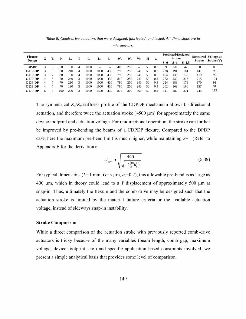
149
Table 8: Comb-drive actuators that were designed, fabricated, and tested. All dimensions are in
micrometers.
Flexure
Design G Tf N Lf T L L2 L3 W1 W2 W3 H a0
Predicted/Designed
Stroke Measured
Stroke
Voltage at
Stroke (V) S=0 S=1 S=1.5
DP-DP 3 6 50 150 4 1000 -- -- 400 250 -- 50 0.5 59 50 47 50 85
C-DP-DP 3 9 80 210 4 1000 1000 430 790 250 240 50 0.2 228 191 181 141 95
C-DP-DP 3 7 80 180 4 1000 1000 430 790 250 240 50 0.5 164 138 130 119 90
C-DP-DP 4 8 70 240 3 1000 1000 430 810 250 240 50 0.2 272 230 218 215 104
C-DP-DP 4 7 70 210 3 1000 1000 430 790 250 240 50 0.3 224 188 178 170 91
C-DP-DP 4 7 70 190 3 1000 1000 430 780 250 240 50 0.4 202 169 160 157 91
C-DP-DP 6 8 100 290 3 1000 1500 430 875 300 360 50 0.2 341 287 271 245 119
The symmetrical Kx/Ky stiffness profile of the CDPDP mechanism allows bi-directional
actuation, and therefore twice the actuation stroke (~500 m) for approximately the same
device footprint and actuation voltage. For unidirectional operation, the stroke can further
be improved by pre-bending the beams of a CDPDP flexure. Compared to the DPDP
case, here the maximum pre-bend limit is much higher, while maintaining S=1 (Refer to
Appendix E for the derivation):
0 2
11 11
4ypr
GLU
k k
(5.39)
For typical dimensions (L=1 mm, G=3 µm, a0=0.2), this allowable pre-bend is as large as
400 µm, which in theory could lead to a Y displacement of approximately 500 µm at
snap-in. Thus, ultimately the flexure and the comb drive may be designed such that the
actuation stroke is limited by the material failure criteria or the available actuation
voltage, instead of sideways snap-in instability.
Stroke Comparison
While a direct comparison of the actuation stroke with previously reported comb-drive
actuators is tricky because of the many variables (beam length, comb gap, maximum
voltage, device footprint, etc.) and specific application based constraints involved, we
present a simple analytical basis that provides some level of comparison.

150
At large displacements, we can approximate the bearing direction stiffness of the CDPDP
mechanism by equation (5.27). With this stiffness, equation (5.24) can be rewritten as:
3
32
max max30 2
11 11
2| 6
1y
LU NV L
E Tk k S
(5.40)
Here S is no longer assumed to be 1 instead, it is retained as a function of the error
motions Ex, given in (1.16). It can be separately shown that for most flexure mechanisms
based on the parallelogram module (e.g. P, DP-DP, C-DP-DP, etc.) that are used in
comb-drive actuation, a relation analogous to the above equation can be derived.
However, for devices with pre-bend, the above relation has to be revised. We can still
neglect the elastic stiffness term (1/k33) w.r.t. the elasto-kinematic term to obtain a
relation similar to that in equation (5.27) (Appendix EAppendix E):
2
23 2
11 0
42 zz
x
y ypr
EI LK
L U U k a
(5.41)
Thus, equation (5.40) can be rewritten as:
3
22
max max max30 2
11 11
2| | 6
1y y ypr
LU U U NV L
E Tk k S
(5.42)
The goal is to maximize the left hand side of the equation for a fixed set of device and
material parameters N, V, L, T, ε and E. This implies comparing the second non-
dimensional term on the right hand side of the above expression which entirely captures
the flexure stiffness and error motion properties. As all of the devices that we are
considering are silicon based and operated in air, the permittivity and young’s modulus
do not vary significantly and hence are included in the second term. Thus, in figure, we
plot (Uy|max (Uy|max-Uypr)2)1/3
vs (NV2
maxL4/T
3)1/3
for in-plane comb-drive actuators
reported in previous literature. The performance of a given device can be estimated by

151
comparing the slope that it makes at the origin of the plot. The Figure 79 shows a
significant performance improvement offered by the CDPDP mechanism.
DP-TDP Optimization
For this device, we would consider a layout shown in Figure 71 similar to that used for
the CDPDP actuator in the previous section. As before, we can use the rigorous
numerical optimization method to come up with the dimensions of the device. As
mentioned before, this mechanism exhibits finite error motions and hence, none of the
simplified snap-in conditions (equations(1.6), (1.7) and (1.14)) can be used in this case.
Therefore, we would have to resort to using the numerical solution procedure
summarized in chapter 1 (equations) to obtain the stroke at snap-in. Moreover, we would
have to include finite element analysis in the optimization loop as well to calculate the
stiffness and error motions of the mechanism for every set of parameters (W1, W2, α, β, T,
a0, L). Needless to say, this increases the complexity of the problem several fold. A
closed form parametric solution for the characteristics of the flexure mechanism can
simplify the solution procedure significantly.

152
a
b
2W2
Rt
(L,a0)
2W1 Tf G
Lf
Ground, Fixed Anchor
N Fingers
Ground, Fixed Anchor
α
β
(L,a0)
Figure 71: The DP-TDP comb drive actuator layout
We would not pursue the above approach here but use a fairly simplified graphical
method to arrive at an approximate solution. Only the tilt angles α and β are chosen as
variables and the rest of the dimensions of the flexure are the same as those considered in
chapter 4. Thus, we can directly use the FEA plots of stiffness and error motions from the
same discussion in the design of this actuator. From these results, we previously
concluded that a value of α close to β would give the best characteristics of the
mechanism. In this section, we take this a step further and with appropriate
approximations, converge on values of α and β that give near-optimal performance i.e. a
large stroke for low actuator effort. To begin, we choose a sector around the α=β line
such that the x-error motions are less than the gap size. This sector is the shaded region
shown in the contour plot (Figure 72) of Figure 38 for a gap size of 5 μm.

153
-2e-05
-2e-05
-1.5e-05
-1.5e-05
-1e-05
-1e-05
-1e-0
5
-5e-06
-5e-06
-5e-06
-3e-06
-3e-06
-3e-0
6
-3e-
06
0
0
0
0
3e-0
6
3e-0
6
3e-06
5e-0
6
5e-0
6
5e-06
1e-0
5
1e-0
5
1.5
e-0
5
1.5
e-0
5
2e
-05
E
x (X-Error motions for U
y=0.2L)
0.05 0.1 0.15 0.2 0.25
0.05
0.1
0.15
0.2
0.25
`
Figure 72: Contour plot of Ex(m) for the DP-TDP mechanism. The tilt angles are in radians.
Inspecting Figure 72, Figure 73, Figure 74 and Figure 75, we can further narrow down
the optimal space to α, β>0.1. In this region, Figure 73 shows that Eθ≤0.0005. Assuming
Lf and hence Loff for the layout shown in Figure 71 to be around 200 μm, we find that Loff
Eθ≤0.1 μm which is much smaller (<2%) in comparison to the gap size. Referring to
equations (1.9) and (1.10), this implies that we can neglect the effect of the rotational
error motions on the snap-in conditions. Moreover, Figure 76 shows that the ratio
between Kθ and KxL2
off is always greater than 5 in the feasible space and hence, for the
first iteration we can use a purely one dimensional model for snap-in. We can thus,
directly plot (Figure 77) the metric given in equation (1.18) i.e. Kx/(1+S)K3
y and choose
the configuration corresponding to the maxima in the plot. The maximum occurs at
α=0.14 and β=0.17 radians. For these dimensions, the stroke obtained is around 154
microns.
Beyond this point, we can redraw plots for the error motions and stiffness at Uy=154
microns and obtain new values of the tilt angles and subsequently the updated stroke. We

154
can then repeat the process till we converge on a set of tilt angles and the corresponding
stroke. Moreover, we can use the one dimensional snap-in model for the subsequent
iterations as well as none of the assumptions get violated in this displacement range. For
these dimensions, the optimal tilt angles obtained before do not change significantly in
the subsequent iterations.
-0.0
03
-0.0
02
-0.0
02
-0.0
01
-0.0
01
-0.0
005
-0.0
005
-0.0
005
-0.0
001
-0.0
001
-0.0
001
0
0
0
0
0.0001
0.0001
0.00
01
0.00
01
0.0005
0.0005
0.0005 0.001
0.001
0.001
0.002
0.002
0.002
0.003
0.003
0.0040.004
Eq (q Error motions for U
y=0.2L)
0.05 0.1 0.15 0.2 0.25
0.05
0.1
0.15
0.2
0.25
Figure 73: Contour plot of Eθ (in radians) for the DP-TDP mechanism.

155
0.48
0.48
0.48
0.48
0.48
0.48
0.48
0.5
0.5
0.5
0.5
0.5
0.5
0.5
0.5
5
0.55
0.55
0.55
0.55
0.6
0.6
0.6
0.6
0.6
0.65
0.65
0.65
0.6
5
0.6
5
0.7
0.7
0.7
0.7
0.75
0.75
0.7
5
0.8
0.8
0.8
0.85
0.9
K
y (Motion Direction Stiffness for U
y=0.2L)
0.05 0.1 0.15 0.2 0.25
0.05
0.1
0.15
0.2
0.25
Figure 74: Contour plot of Ky (in N/m) for the DP-TDP mechanism.
100
100
100
200
200
200
300
300
300
400
400
400
500
500
500
50
0
600
600
60
0
600
Kx (x-direction stiffness for U
y=0.2L)
0.05 0.1 0.15 0.2 0.25
0.05
0.1
0.15
0.2
0.25
Figure 75: Contour plot of Kx (in N/m) for the DP-TDP mechanism.

156
5
5
10
10
10
10
10
10
20
20
20
30
30
30
40
4040
50
50
10015
020
0
Kq/(L
off
2 K
x)
0.05 0.1 0.15 0.2 0.25
0.05
0.1
0.15
0.2
0.25
Figure 76: Contour plot of Kθ/(KxL2off) for the DP-TDP mechanism.
Maximum
Figure 77: Plot of the objective function for Uy=0.2L. The maximum occurs at α=0.14, β=0.17. The(1+ S)
used here is simply the theoretical factor due to axial error motion (Ex) and does not include the effect of
imperfections

157
For the actual devices that were fabricated and tested in [36], tilt angles were chosen as
α=0.11 and β=0.1411 while keeping all other dimensions the same as before. The
predicted stroke with these dimensions is 141 microns which is not significantly different
from that obtained with α=0.14 and β=0.17. The measured actuation stroke at snap-in for
the conventional DP-DP flexure with the above dimensions was 75 µm at 45 volts. The
actuation stroke for a DP-TDP flexure with the same dimensions was measured to be 125
µm at 70 volts. As expected, an even higher stroke of 149 µm was measured for a DP-
TDP flexure with the same overall dimensions but using reinforced beams (a0 = 0.2). On
comparison with the predicted actuation stroke (Table 9), these experimental
measurements also show that for the DP-DP flexure because of symmetry, a stability
margin of S = 0 is acceptable. However, because of asymmetry in the DP-TDP
maintaining a stability margin of S = 1 is necessary.
Table 9: Comb-drive actuators that were micro-fabricated and tested. Comb-drive dimensions are same in
all cases: G = 5 m, comb-finger length Lf = 190 m, in-plane thickness Tf = 6 m, out-of-plane thickness
Hf = 50 m, and N = 70. Flexure beam length L = 1000 m and in-plane thickness T = 3 m in all cases.
All dimensions are in microns.
Flexure
Design W1 W2 a0
Designed
Stroke Measured
Stroke
Voltage
(V) S=0 S=1
DP-DP 450 250 0.5 76.7 54.2 75 45
DP-
TDP 525 325 0.5 141 122 125 70
DP-
TDP 525 325 0.2 178 156 149 86
11 These values were obtained with a coarser mesh of α and β

158
Figure 78: SEM image of micro-fabricated comb-drive actuators based on the DP-DP and DP-TDP
flexures.
0 1 2 3 4 5 6 7 8 9
x 105
0
50
100
150
200
250
(NVmax
2L
4/T
3)1/3
Volt2/3
m1/3
Equiv
ale
nt
str
oke(
m)
= (
Uy| m
ax(U
y| m
ax-U
ypr))
1/3
Brouwer, 2010
Grade, 2003
Chen, 2003
Awtar, CDPDP, 2012
Legtenberg, 1996
Hou, 2006
Awtar, CDPDP, 2012
Awtar, DP-TDP, 2012
Awtar, DP-TDP, 2012
Grade, 2004
Zhou, 2004
Figure 79: Performance comparison between different comb drive actuators. The references are as follows:
Legtenberg, 1996 [33], Chen, 2003 [66], Grade, 2003 [34], Grade, 2004 [67], Zhou, 2004 [37],
Hou, 2006 [68], Brouwer, 2010 [54], Awtar, CDPDP 2012 [32], Awtar, DP-TDP [36]
Secondary Stage
Motion Stage
1 mm
DP-DP
DP-TDP
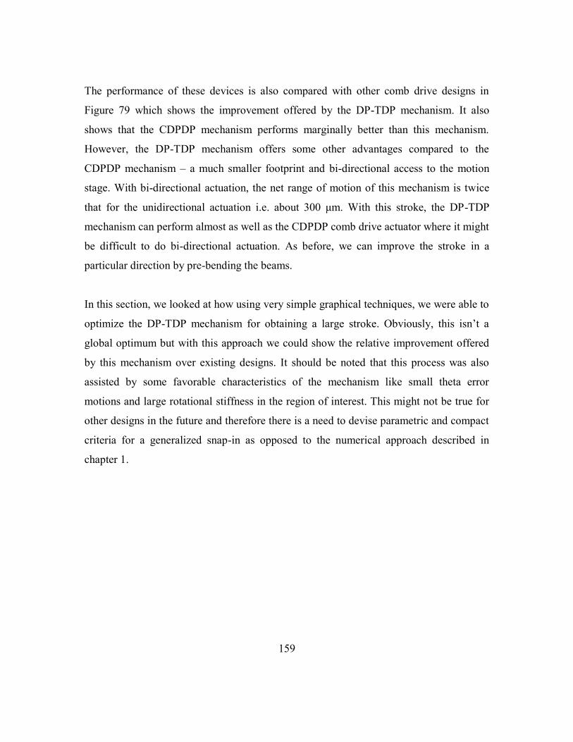
159
The performance of these devices is also compared with other comb drive designs in
Figure 79 which shows the improvement offered by the DP-TDP mechanism. It also
shows that the CDPDP mechanism performs marginally better than this mechanism.
However, the DP-TDP mechanism offers some other advantages compared to the
CDPDP mechanism – a much smaller footprint and bi-directional access to the motion
stage. With bi-directional actuation, the net range of motion of this mechanism is twice
that for the unidirectional actuation i.e. about 300 μm. With this stroke, the DP-TDP
mechanism can perform almost as well as the CDPDP comb drive actuator where it might
be difficult to do bi-directional actuation. As before, we can improve the stroke in a
particular direction by pre-bending the beams.
In this section, we looked at how using very simple graphical techniques, we were able to
optimize the DP-TDP mechanism for obtaining a large stroke. Obviously, this isn’t a
global optimum but with this approach we could show the relative improvement offered
by this mechanism over existing designs. It should be noted that this process was also
assisted by some favorable characteristics of the mechanism like small theta error
motions and large rotational stiffness in the region of interest. This might not be true for
other designs in the future and therefore there is a need to devise parametric and compact
criteria for a generalized snap-in as opposed to the numerical approach described in
chapter 1.

160
Chapter 7: Conclusions and Future Work
Contributions
The specific contributions of this thesis are summarized below:
1. Development of metrics for comparison of the bearing behavior of single axis
planar flexure mechanisms. These were the range of motion, error motions, the
motion direction stiffness and the bearing direction stiffness. These offer
estimates of only the static or quasi-static performance of the flexure mechanism
with scope for incorporating additional metrics for the dynamic performance
without reformulating the existing ones. A bearing is said to perform well if it
offers a large range of motion, small or negligible error motions, small motion
direction stiffness and large bearing direction stiffness. Moreover, some
applications such as comb drive and voice coil actuators were discussed where
these quantities directly affect the behavior of the devices.
2. These metrics were then quantified for some existing flexure mechanism i.e. the
parallelogram (P), double parallelogram (DP) and lever double parallelogram (L-
DP) for which some additional results were derived based on the existing beam
constraint model. These include expressions for the yield criterion of a flexure
which limits the range of motion and derivation of the error motion and stiffness
characteristics from the force displacement relations derived previously. Where
force-displacement relations were not available like in the case of the L-DP
mechanism, a qualitative analysis of the performance metrics was done using
extensive FEA analysis for various configurations and dimensions of the
mechanism.

161
3. Some variations of these flexure mechanisms were also discussed which do not
alter the overall topology of the mechanism like the reinforced beam flexure and
the multi-beam parallelogram. Wherever necessary, additional results were
derived for the metrics of the mechanisms which incorporate these variations.
Moreover, the influence of these modifications on the metrics is also examined to
come up with criteria that can further boost the performance of the mechanism.
4. The non-linear strain energy formulation for flexure mechanism that is consistent
with the beam constraint model was also revisited for the existing mechanisms.
An algorithm was developed to simplify the total strain energy expression for
these mechanisms based on order of magnitude estimates, which were obtained
using the BCM model and/or finite element analysis for the displacement and
dimensional variables involved. This was done in a manner that preserves the
force displacement relations that one obtains by applying the principle of virtual
work on the actual strain energy expression. This algorithm was then applied to
the two-beam and the multi-beam parallelograms to obtain the exact same
expressions that were derived using the BCM model.
5. Force-displacement relations for the CDPDP mechanism were derived using the
direct BCM model. Appropriate assumptions were made wherever required with
justifications to simplify the solution procedure. The obtained relations agreed
with finite element predictions for a wide range of dimensions. The sources for
any discrepancies were also identified and some measures were suggested which
could be used to eliminate them. The relations were extended to incorporate beam
reinforcement and multi-beam parallelograms. Finally, some guidelines were laid
out for choosing the dimensions of the mechanism in order to obtain optimum
performance.

162
6. The characteristics of the DP-TDP mechanism were discussed qualitatively using
finite element analysis in a manner analogous to that for the L-DP mechanism.
The difficulties that might be encountered while trying to obtain a closed form
parametric solution were also discussed. Some critical dimensions of the
mechanism were identified and were used in the parametric FEA. Based on the
results, some estimates were made for the optimum choice of these dimensions to
obtain the best possible performance.
7. Detailed design, fabrication, assembly and testing of a low cost, reconfigurable
and high precision setup to directly measure the properties of the CDPDP
mechanism in order to validate the force displacement relations derived before
was discussed. One of the possible configurations is the DPDP mechanism and
therefore, using the same setup, one could show the performance improvement
offered by the CDPDP mechanism. A complete error analysis was done to
examine the effect of fabrication imperfections and measurement uncertainties on
the stiffness and error motions of the mechanism.
8. As a case study, systematic methods to design a flexure mechanism as a motion
guide for a comb drive actuator were laid out with the objective of maximizing
the stroke for given footprint and voltage specifications. With the analytical
framework for the CDPDP mechanism already presented, the design approach for
the CDPDP mechanism was more detailed and deterministic. However, for the
DP-TDP mechanism, due to the lack of parametric results for the stiffness and
error motions, only a first-pass analysis was done with only a few dimensions
chosen as the variables while others chosen almost arbitrarily at the onset of the
procedure. MEMS comb drive actuators based on the device designs obtained
from these procedures were then fabricated and tested as a part of a separate

163
project by Dr. Mohammad Olfatnia12. It was found that the CDPDP flexure
offered a very large stroke of 245 microns and the DP-TDP gave a stroke of 145
microns which are about 5 and 3 times respectively larger than that given by the
DPDP mechanism for the same dimensions.
9. A need for a reliable metric for the comparison of the performance of different
flexure mechanisms in a comb drive actuator was soon identified. Thereafter, a
metric was defined which offers a good measure of comparison between the
flexure mechanisms that have been considered in this thesis. Based on this metric,
it was found that the CDPDP and the DP-TDP mechanisms offer significantly
improved performance over the previously reported comb drive devices.
Moreover, the CDPDP mechanism performs marginally better than the DP-TDP
mechanism. However, the DP-TDP mechanism makes up for this shortcoming by
offering a lower footprint and bi-directional access to the motion stage, which
might not be possible in the CDPDP mechanism.
Future Work
In this thesis, it was shown how some valuable insights into the nature of a mechanism
can enable us to make some approximations which can significantly simplify the
equations describing the characteristics of the mechanism thereby making closed form
solutions possible in many cases. A theoretical framework has been created which allows
for a lot of scope for future work in this area. Some of the foreseeable work that can be
done to improve upon or extend the ideas that have been presented in this thesis is listed
below:
1. A metric for the dynamic behavior of flexure mechanisms has to be created which
could incorporate resonant frequencies, modes and structural damping. For comb-
12 Department of Mechanical Engineering, University of Michigan, Ann Arbor

164
drive actuators this would give a measure of the bandwidth of the device.
Obviously, there is a direct tradeoff between bandwidth and stroke, and with this
metric in place, we could do a multi-objective optimization to maximize the
stroke and the bandwidth instead of just the stroke like we did in chapter 6.
2. Closed form solutions for the system of equations obtained for the DPDP and the
CDPDP mechanisms by applying the principle of virtual work could be obtained
by applying further approximations on the strain energy expressions for each of
these mechanisms. Also, instead of using the parallelogram as the building block,
one could use the double parallelogram mechanism as a higher level block for
more complex mechanisms. Unlike the parallelogram, the double parallelogram
would be a two input-one output block where the two inputs would be forces at
the primary and the secondary stages and the output would be the displacement at
the primary stage. This would mean that the strain energy would be a function of
the forces at the secondary stage and the displacements at the primary stage.
Alternatively, one could use the principle of complementary virtual work which
would simplify the solution for serial configurations significantly. However, for
parallel systems, as before, the problem would again culminate to solving a
system of simultaneous multivariate polynomial equations in terms of the force
variables which might again prove to be difficult to do in closed form. Hence, for
systems which contain both serial and parallel elements, we have to come up with
a hybrid solution procedure which combines elements from both the approaches.
3. An approximate closed form solution for the DP-TDP mechanism can be obtained
for a narrow domain of tilt angles for which the error motions are small. In that
case, the kinematic conflict between the two halves of the mechanism would be
minimal and so would the internal forces and moments. This in turn would mean
that the BCM relations would be valid and can be used to solve for the
characteristics of the mechanism.

165
4. A setup similar to that used for the CDPDP mechanism can be used to validate the
stiffness and error motions of the DP-TDP flexure. In fact, one could use the same
measurement techniques and replace the plate containing the CDPDP mechanism
with a plate carrying a different design.

166
Appendix A
BCM COEFFICIENTS AS FUNCTIONS OF BEAM REINFORCEMENT A0
Coefficien
t Function Plot
0
11k 2
0 0 0
6
3 6 4a a a
0
12k 2
0 0 0
3
3 6 4a a a
0
22k
2
0 0
2
0 0 0
3 3 2
3 6 4
a a
a a a
0 0.1 0.2 0.3 0.4 0.50
50
100
150
200
250
a0
Coeffic
ient
0 0.1 0.2 0.3 0.4 0.5-120
-100
-80
-60
-40
-20
0
a0
Coeffic
ient
0 0.1 0.2 0.3 0.4 0.50
20
40
60
80
100
120
a0
Coeffic
ient

167
1
11k
2 3
0 0 0
22
0 0
3 15 50 60 24
5 3 6 4
a a a
a a
1
12k
2 3
0 0 0 0
22
0 0
15 60 84 40
5 3 6 4
a a a a
a a
1
22k
2 3 4
0 0 0 0 0
22
0 0
4015 60 92 60
3
5 3 6 4
a a a a a
a a
2
11k
3 2 3 4
0 0 0 0 0
32
0 0
2 105 630 1440 1480 576
175 3 6 4
a a a a a
a a
0 0.1 0.2 0.3 0.4 0.51
1.05
1.1
1.15
1.2
a0
Coeffic
ient
0 0.1 0.2 0.3 0.4 0.5-0.1
-0.08
-0.06
-0.04
-0.02
0
a0
Coeffic
ient
0 0.1 0.2 0.3 0.4 0.50
0.02
0.04
0.06
0.08
0.1
0.12
0.14
a0
Coeffic
ient
0 0.1 0.2 0.3 0.4 0.5-1.5
-1
-0.5
0x 10
-3
a0
Coeffic
ient

168
2
12k
3 2 3 4
0 0 0 0 0
32
0 0
105 630 1440 1480 576
175 3 6 4
a a a a a
a a
2
22k
3 2 3 4 5 6
0 0 0 0 0 0 0
32
0 0
1120105 630 1560 2000 1408 560
9
175 3 6 4
a a a a a a a
a a
33k 2
0
6
a t
0 0.1 0.2 0.3 0.4 0.50
1
2
3
4
5
6
7
8x 10
-4
a0
Coeffic
ient
0 0.1 0.2 0.3 0.4 0.5-0.4
-0.35
-0.3
-0.25
-0.2
-0.15
-0.1
-0.05
0
a0
Coeffic
ient
0 0.1 0.2 0.3 0.4 0.50
5
10
15x 10
5
a0
Coeffic
ient

169
Appendix B
JUSTIFICATION AND GUIDELINES FOR APPROXIMATIONS USED IN THE DERIVATION OF
THE STIFFNESS EXPRESSIONS FOR THE CDPDP MECHANISM
Rotational stiffness of the clamp parallelograms (Equation (4.5))
Using equation (3.35), the non-dimensional rotational stiffness for the parallelograms in
the clamp would be given as:
3
3 3
2 23 (2)3 1
112 2
3 3
2
12
12x
EH TK
L T Uk
L L
q
(B.1)
Using equation (4.9) for Ux1 and obtaining the ratio between the elastic and the elasto-
kinematic terms in the denominator:
2 2 2
3 3 3
2 222 1 22 41 11 1 2 11 11
11 11
16
12 3112
2 4
x y y
T T tElastic
Elasto kinematic U k U k k uk k
L
(B.2)
Using the estimates given in Table 3, this ratio comes out to be of the O(102) and hence,
we can neglect the elasto-kinematic component.
Motion direction stiffness of the clamp parallelograms (equation (4.6))
Using equation (3.32), the motion direction stiffness of the clamp parallelograms can be
written as:
230 1 1 33 3
11 113 3
3 3 3
122
12
y
y
F LEH TK k k
L EH T
(B.3)
The force Fy1 can be obtained using equations (4.11) and (4.20):
1311
1 2 0
1112 2 2
x y
y
f k uEHTF
L k
(B.4)
Obviously, this force is largest when η=∞ when its value is given by:

170
3
1
1 max 112|
24y x y
EHTF f k u
L
(B.5)
Substituting this value in equation (B.3) and comparing the two terms, we get:
20 3
3 311
2 31
3 311
2Nominal
Stiffening 0.5 x y
H Tk L
L HTk f u
(B.6)
Using some typical values given in Table 3 and a value of L3=0.6L (which does not cause
appreciable stiffening in the motion direction of the entire mechanism), this ratio comes
out to be of O(102) which implies that the stiffening term can be neglected from the
motion direction stiffness.

171
Appendix C
UPPER BOUND ON THE CLAMP EFFECTIVENESS IMPOSED BY FINITE ROTATIONAL STIFFNESS
OF THE DP UNITS IN THE CDPDP MECHANISM
In the derivation for the bearing stiffness of the CDPDP mechanism, we imposed no
constraints on the maximum value that the effectiveness can take, assuming that we can
make it arbitrarily large with η→∞. However, this is not true and we would see shortly
that the maximum effectiveness of the clamp is directly related to the rotational stiffness
of the DPDP unit that it is meant to constrain. This effect explains the small
discrepancies between the stiffness predicted by the model and FEA (Figure 33).
The primary assumption that we made in the closed-form derivation of the bearing
stiffness was that the rotational stiffness of the DP units is very large, so large that the
rotation of the secondary stage is negligible compared to that of clamp (θz1, θz2<< θz3).
This is true for small values of effectiveness but fails for larger values when the rotational
stiffness of the clamp becomes comparable to that of the DP units. This scenario is
depicted in Figure 34.
To simplify the analysis, we assume symmetry between the two halves of the mechanism
i.e. θz1≈ θz2. Moreover, we can say that equation (4.4) still holds approximately. Thus,
rewriting equation (4.5):
2 2 2 2
3 0 3 2 3 3 0 3 1 33 2 3 12 2 3 2 2 3
3 3 3 3 3 3 3 3
2
3 3 31 2 3 1
0 3
12 12
2 6 2 6
c c
z zz z z z
z z z zc
L a T M L L a T M L
W L EH T W L EH T
EH T WM M
a L
q q q q
q q
(C.1)
Now, the moment Mz1 applied on the secondary stage results in a rotation θz1. The
rotational stiffness of the secondary stage with the primary stage constrained is simply

172
given as the sum of the rotational stiffness of the outer and the inner parallelograms of the
DP unit i.e.
1 12 2
2 22 22 1 2 10 0 1
11 0 11 0 12 2 2 2 3
1 2
12
2 6 2 6
y y zz
U UT a T a M LL Lk a k a
W L L W L L EHTq
(C.2)
Assuming that the clamp constrains the Y-displacement of the secondary stages to close
to half that of the primary stage i.e. Uy1≈0.5Uy, we can rewrite the above equation:
22201
1 11 0 13 2 2
1 2
3 1
3 2
yzz z
UT aM Lk a M
EHT W Wq
(C.3)
Substituting this relation in equation (C.1), we get:
2
3 3 3
0 3
1 32
3 3 3
0 3
1
c
z z
c
EH T W
a LM
EH T W
a L
q
(C.4)
Finally, using equations (4.3) and (4.4) while neglecting the contribution of Fx1, we get:
2
3 3 3
2 10 3
1 2223 3 3
0 32
3 3 3
30 3
1 1 2 3 2223 3 3
0 3
21
6,
1
cy y
y
c
c
y eff y y eff
c
EH T W
U Ua LF
LEH T W
a L
EH T W
a L Lf u u
EHT LEH T W
a L
(C.5)
This shows that as we make the rotational stiffness of the clamp very large, the actual
effectiveness becomes proportional to the ratio 1/κ which is the rotational stiffness of the
DP units at the secondary stage. Figure 80 shows the comparison between the FEA and
the theoretical values with the revised expression for effectiveness (equation (C.5)) for
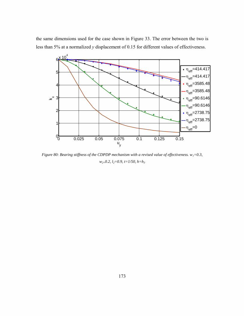
173
the same dimensions used for the case shown in Figure 33. The error between the two is
less than 5% at a normalized y displacement of 0.15 for different values of effectiveness.
Figure 80: Bearing stiffness of the CDPDP mechanism with a revised value of effectiveness. w1=0.3,
w2=0.2, l2=0.9, t=1/50, h=h3
0 0.025 0.05 0.075 0.1 0.125 0.150
1
2
3
4
5
6x 10
4
uy
kx
eff
=414.417
eff
=414.417
eff
=3585.48
eff
=3585.48
eff
=90.6146
eff
=90.6146
eff
=2738.75
eff
=2738.75
eff
=0

174
Appendix D
NOTES ON THE CENTER OF STIFFNESS OF THE CLAMPED PAIRED DOUBLE
PARALLELOGRAM MECHANISM
Location of the COS
The CDPDP mechanism with a possible offset between the centers of the primary and
secondary stages, shown in figure is used for this analysis. In order to simplify the
analysis, we would only consider the case of a near-ideal clamp such that Uy1=Uy2≈0.5Uy.
With this assumption, we can remove the clamp from figure and replace it with
appropriate forces (given by equation (3.69) for a DPDP mechanism) and moments given
by:
1
1 11 11
1 1
y y x
z y
f u k f
m f
(D.1)
Woffset
T3(L3,a
0c )
Clamp
GroundAnchor
Rigid Link
2W3
2L2
(Fy,Uy)
(Fx, Ux)
(Mz, θz)
(L,a0)
2W1
2W2 Woffset
(Fy,Uy)
(Fx, Ux)
(Mz, θz)
Fy1Mz1
(L,a0)
2W1
2W2
Mz1Fy1
Ux1
θz1
0.5Uy
Ux2
0.5Uy
θz2
(Fy11,Uy)
(Fx11, Ux)
(Mz11, θz) (Fy22,Uy)
(Fx22, Ux)
(Mz22, θz)
Figure 81: The simplified model of a near-ideal CDPDP mechanism
Rewriting equation (3.52) for this configuration:

175
2 0 1(2)
1 11 11 1 11 11 12 11 122
1 33
2(2) (0) (1)
11 11 12 11 122
2 33
2(2)
1 11 22 1 22 222
1 33
1 1| 0.5 0.5 0.5 2
2
1 10.5 0.5 (2 )
2
1 1| 0.5
2
z DP y z z y x offset y y x
y z y x
z DP y z z y x
u k m m f f w u u k f kw k
u k m u k f kw k
u k m m f fw k
q
q
0 1
12 22 12
2(2) (0) (1)
11 22 12 22 122
2 33
0.5 0.5 2
1 10.5 0.5 (2 )
2
offset y y x
y z y x
w u u k f k
u k m u k f kw k
(D.2)
Moreover,
1 2| |z DP z DPq q (D.3)
In order to calculate the center of stiffness, we would apply a force fx at different
locations on the primary stage and determine the location at which θz goes to zero. We
can resolve this force to a force fx and a moment -fxd applied at the center of the stage
where d is the distance of the force from the center of the primary stage. Thus, using
results derived in Chapter 4, we have:
11 22
11 22
10 11
11 11 0
111
0 1122 11 0
11
0.5
14
14
z z x
x x x
xy y
xy y
m m f d
f f f
k ff k u
k
k ff k u
k
(D.4)
Equations (D.1) to (D.4) can be solved to obtain:
2
1 2 1 2, , , , , , , ,z x offset y offset y xf p w w w t u q w w w t u d O fq (D.5)
Using the definition of the COS:

176
2
1 2 1 2 cos
1 2 ,
cos
1 2 ,
0 , , , , , , , ,
, , ,
, , ,
z x offset y offset y x
offset y
offset y
f p w w w t u q w w w t u d O f
p w w w t ud
q w w w t u
q
(D.6)
Where the functions p and q are given below:
2 22 2 2
1 2 11 33 1 11 33
1 1 2 2 2
11 11 11 33 21 2 2 2 2
12 11 33 1 2
2
2, , , , (1 0.25 )( )(( (0.25 0.0625 )
(0.125 0.125 (0.03125 0.03125 ) ))
(0.125 0.03125 )( ))
offset y y offset y
y y
y y
p w w w t u k k u w w k k u
u k k k k u w
k u k k u w w
w
(D.7)
2 22 2 4
1 2 11 33 11 33 1
2 22 2 2 2
11 33 11 33 1 22 22 2 4
11 33 11 33 2
, , , , ( 0.25 ( 0.125 0.015625 ))
( 0.5 ( 0.25 0.03125 ))
( 0.25 ( 0.125 0.015625 ))
offset y y y
y y
y y
q w w w t u k k u k k u w
k k u k k u w w
k k u k k u w
(D.8)
This closed form result matches very well with corresponding FEA results as shown in
Figure 82.
Figure 82: Comparison between theoretical (linear model) and FEA COS for w1=1.0, w2=0.8,
t=0.0123,woff=0.1, w3= 0.5, l3=0.3. Almost no sensitivity was observed w.r.t. fx.
0 0.02 0.04 0.06 0.08 0.1-0.08
-0.075
-0.07
-0.065
-0.06
-0.055
-0.05
-0.045
-0.04
-0.035
uy
dco
s
Theoretical
FEA
177
Woffset
Fy1Mz1
2W1
2W2
Mz1Fy1
Ux1
θz1
0.5Uy
Ux2
0.5Uy
θz2
(Fy11,Uy)
(Fx11, Ux)
(Mz11+ΔMz, θz) (Fy22,Uy)
(Fx22, Ux)
(Fy,Uy)
(Fx, Ux)
(Mz, θz)
CL
(Mz22-ΔMz, θz)
Figure 83: Special case of the CDPDP design.
For the case shown in Figure 83, an extra moment would be applied on each double
parallelogram by the motion direction force Fy and this moment would be given by:
110.5z y LM F C (D.9)
Using the same procedure as before, the new center of stiffness would be given by:
1 22
11 12 1 1 2
cos 11 122 2 2 2
1 2 1 2
1 2
10.5 0.25 0.5 1
2, , , , ,
offs
offse
e
t yl y
t
l y
k ww w w c t u
w wd c k k u O u
w w w w
(D.10)
The higher order uy terms were observed to be small enough to be ignorable.
X-direction displacement at COS
In our derivation of the axial stiffness of the CDPDP mechanism, we neglected the
contribution of the rotation of the parallelograms in the x-direction relations i.e.
approximate decoupling between the x,y and θ direction relations. However, for the case
shown in Figure 83, this might not be true due to the presence of an offset between the

178
COS of outer parallelogram and the location of the COS of the CDPDP mechanism on
the primary stage. This scenario is shown in Figure 84.
Woffset+0.5Uy
Fy1Mz1
(Fx11, Ux)
CL
X
θz=0
Dcos
(Fy11, Uy)
D1cos
θz11≠0
Uxθ
X
Figure 84: Right half of the CDPDP mechanism when a force is applied exactly at the COS
Using the previous analysis for determining the location of the COS, the rotation θz1 of
the secondary stage can be easily calculated13. The additional displacement Uxθ would
then be:
1 1cos cos0.5x z offset y
x x decoupled x
u d w u d
u u uq
q
q
(D.11)
Where d1cos is the location of the COS of the outer parallelogram. In order to calculate
this, we can rewrite equation (3.3) for the rotation of the parallelogram and equate it to
zero:
13 The equation is too long to be listed here. It can be found in ‘’

179
2
(2) (0) (1)
11 11 1cos 12 11 122
1 33
(0) (1) (0) (1)
12 11 12 12 12
1cos
11
1 10 [ 0.5 (2 )]
2 4
0.5 (2 ) 0.5 (2 0.5 )
0.5
y
x y x
y x y
x x
uk f d u k f k
w k
u k f k u k kd
f f
(D.12)
Moreover, dcos is COS of the CDPDP mechanism. Using equation (D.11), the new
theoretical value of the stiffness for an applied force fx is:
|
|
xx corrected
xx
x uncoupled
fk
fu
kq
(D.13)
Where kx|uncoupled is given by equation (4.30). For the design shown in Figure 51 the x-
direction stiffness is plotted in Figure 85. The FEA stiffness and the closed-form stiffness
(given by equation (D.13)) match to within 5%.
Figure 85: Closed form and FEA x-direction stiffness for the CDPDP design used in the experiment (Figure
51 )
0.5 1 1.5 2 2.5 3 3.5 4 4.5 5
x 10-3
5.2
5.4
5.6
5.8
6
6.2
6.4
6.6
6.8x 10
7
Uy (m)
Kx (
N/m
)
FEA
Closed Form

180
Appendix E
DERIVATION OF THE LIMIT ON PRE-BENDING FOR COMB DRIVE ACTUATORS
For the x-direction stiffness of the pre-bent CDPDP configuration (with a pre-bend of
Uypr), we can use an approximation similar to that given by equation (5.27). However, the
limit on the thickness would now be lower than that given by equation (5.26). Assuming
that the thickness is larger than this limit so that the ratio between the elastic and elasto-
kinematic terms is larger than 5% but still lower than 10%, or in other words, the elastic
term is ε times (where 0.05<ε<0.1) the elasto-kinematic term at the snap in point Uy|max
i.e.
2
max 2
11 03 233 0
max 2
11 0
33 0
2
2 23 3 2
max max 11 02
11 0
|1 12 :
4|1
4
1 42 2 1
| |1
4
y yprzzx
y ypr
zz zzx
y ypr y ypr
u uEIK k a
L k au uk a
k a
EI EI LK
L Lu u U U k ak a
(E.1)
Using the above relation along with the motion direction stiffness given by equation
(5.23) and the axial snap-in criterion given by equation (1.16) with no initial overlap, we
get:
22
max
22 2 0
max 11 11
2 22 2
max max 2 0
11 11
2 2
max max 2 0
11 11
2 22
max max 2 0
11 11
| 42 1 1
|
2 1| |
1
2 1| |
1
2 1| | 0
1
y
y ypr
y y ypr
y y ypr
y ypr y
U LS
G U U k k
G LU U U
S k k
G LU U U
S k k
G LU U U
S k k
(E.2)
The determinant of this quadratic equation is given by:

181
2 2
2
2 0
11 11
2 14
1ypr
G LD U
S k k
(E.3)
The equation will only have two roots i.e. two intersections only (Figure 66) if one of the
determinants is imaginary. This implies that:
2 2
2
2 0
11 11
2 0
11 11
2 14
1
2 12
1
ypr
ypr
G LU
S k k
U GLS k k
(E.4)
Therefore, the critical pre-bend is given by:
2 0 2 0
11 11 11 11
2 1 32| 2 1 0.25
1 1ypr critU GL GL
S k k S k k
(E.5)
This shows that for an ε=0.1, the error in the critical pre-bend is less than 2.5%.
For the DPDP mechanism, the critical pre-bend would be exactly similar with the elasto-
kinematic term k11(2)
getting replaced by the equivalent term for the DPDP mechanism
(equation (3.63)) i.e.:
21
112 0
11 110
11
32|
1
ypr critU GL
kS k k
k
(E.6)

182
References
[1] R. V. Jones, "Some uses of elasticity in instrument design," Journal of Scientific
Instruments, vol. 39, pp. 193-&, 1962.
[2] S. T. Smith, Flexures: Elements of Elastic Mechanisms: Gordon and Breach
Science, New York, 2000.
[3] S. T. Smith, Foundations of Ultra-Precision Mechanism Design: Taylor &
Francis, 2003.
[4] L. C. Hale, "Principles and Techniques for Designing Precision Machines," Ph.D.
Thesis, Mechanical Engineering, Massachusetts Institute of Technology, 1999.
[5] A. H. Slocum, Precision Machine Design. Dearborn, MI: Society of
Manufacturing Engineers, 1992.
[6] G. J. Siddall, "Flexure stage alignment appratus," U.S. Patent 46944777, 1988.
[7] Y. Ando, "Development of three-dimensional electrostatic stages for scanning
probe microscope," Sensors and Actuators A: Physical, vol. 114, pp. 285-291,
Sep 2004.
[8] G. L. Dai, F. Pohlenz, H. U. Danzebrink, M. Xu, K. Hasche, and G. Wilkening,
"Metrological large range scanning probe microscope," Review of Scientific
Instruments, vol. 75, pp. 962-969, Apr 2004.
[9] A. Sinno, P. Ruaux, L. Chassagne, S. Topcu, Y. Alayli, G. Lerondel, S. Blaize, A.
Bruyant, and P. Royer, "Enlarged atomic force microscopy scanning scope: Novel
sample-holder device with millimeter range," Review of Scientific Instruments,
vol. 78, Sep 2007.
[10] A. Weckenmann and J. Hoffmann, "Long range 3 D scanning tunnelling
microscopy," Cirp Annals-Manufacturing Technology, vol. 56, pp. 525-528,
2007.
[11] L. Hongzhong, L. Bingheng, D. Yucheng, T. Yiping, and L. Dichen, "A motor-
piezo actuator for nano-scale positioning based on dual servo loop and
nonlinearity compensation," Journal of Micromechanics and Microengineering,
vol. 13, p. 295, 2003.
[12] C. A. Mirkin, "Dip-pen nanolithography: Automated fabrication of custom
multicomponent, sub-100-nanometer surface architectures," MRS Bulletin, vol.
26, pp. 535-538, Jul 2001.
[13] J. A. Kramar, "Nanometre resolution metrology with the molecular measuring
machine," Measurement Science & Technology, vol. 16, pp. 2121-2128, Nov
2005.

183
[14] A. Sebastian, A. Pantazi, H. Pozidis, and E. Eleftheriou, "Nanopositioning for
probe-based data storage," IEEE Control Systems Magazine, vol. 28, pp. 26-35,
Aug 2008.
[15] R. Duarte, M. R. Howells, Z. Hussain, T. Lauritzen, R. McGill, E. Moler, and J.
Spring, "A linear motion machine for soft x-ray interferometry," presented at the
Optomechanical Design and Precision Instruments, Bellingham, 1997.
[16] S. Henein, P. Spanoudakis, S. Droz, L. I. Myklebust, and E. Onillon, "Flexure
pivot for aerospace mechanisms," in 10th European Space Mechanisms and
Tribology Symposium, Proceedings. vol. 524, R. A. Harris, Ed., ed 2200 Ag
Noordwijk: Esa Publications Division C/O Estec, 2003, pp. 285-288.
[17] S. Henein, P. Spanoudakis, P. Schwab, L. Giriens, L. Lisowski, E. Onillon, and L.
I. Myklebust, "Mechanical slit mask mechanism for the James Webb Space
Telescope spectrometer," in Optical, Infrared, and Millimeter Space Telescopes,
2004, pp. 765-776.
[18] K. H. L. Chau, S. R. Lewis, Y. Zhao, R. T. Howe, S. F. Bart, and R. G.
Marcheselli, "An integrated force-balanced capacitive accelerometer for low-g
applications," Sensors and Actuators A: Physical, vol. 54, pp. 472-476, Jun 1996.
[19] K. D. N., G. Li, and A. C. McNeil, "Single proof mass, 3 axis MEMS transducer,"
U.S. Patent 6845670, 2005.
[20] S. E. Alper, K. M. Silay, and T. Akin, "A low-cost rate-grade nickel
microgyroscope," Sensors and Actuators A: Physical, vol. 132, pp. 171-181, Nov
2006.
[21] C. Tsou and et al., "A novel self-aligned vertical electrostatic combdrives actuator
for scanning micromirrors," Journal of Micromechanics and Microengineering,
vol. 15, p. 855, 2005.
[22] G. A. Roman, G. J. Wiens, and Asme, "MEMS optical force sensor enhancement
via compliant mechanism," in Proceedings of the Asme International Design
Engineering Technical Conferences and Computers and Information in
Engineering Conference 2007, Vol 8, Pts A and B, New York, 2008, pp. 127-135.
[23] S. Awtar, "Synthesis and Analysis of Parallel Kinematic XY Flexure
Mechanisms," Sc. D. Thesis, Mechanical Engineering, Massachusetts Institute of
Technology, 2003.
[24] S. Awtar, A. H. Slocum, and E. Sevincer, "Characteristics of Beam-Based Flexure
Modules," Journal of Mechanical Design, vol. 129, pp. 625-639, 2007.
[25] S. Awtar and A. H. Slocum, "Constraint-based design of parallel kinematic XY
flexure mechanisms," Journal of Mechanical Design, vol. 129, pp. 816-830, Aug
2007.
[26] S. Awtar, J. Ustick, and S. Sen, "An XYZ Parallel-Kinematic Flexure Mechanism
With Geometrically Decoupled Degrees of Freedom," Journal of Mechanisms
and Robotics-Transactions of the Asme, vol. 5, Feb 2013.
[27] J. G. Bednorz, R. L. Hollis, Jr., M. Lanz, W. D. Pohl, and C. E. Yeack-Scranton,
"Piezoelectric XY Positioner," U.S. Patent 4,520,570, 1985.

184
[28] J. Ustick, "Design, Fabrication and Experimental Characterization of a Large
Range XYZ parallel Kinematic Flexure Mechanism," M.S.E. Thesis, Mechanical
Engineering, University of Michigan, 2012.
[29] F. L. Fischer, "Symmetrical three degree of freedom compliance structure," U.S.
Patent 4447048, 1984.
[30] X. Y. Tang, I. M. Chen, and Ieee, "A large-displacement and decoupled XYZ
flexure parallel mechanism for micromanipulation," presented at the 2006 IEEE
International Conference on Automation Science and Engineering, Vols 1 and 2,
New York, 2006.
[31] L. L. Howell, Compliant mechanisms, 2001.
[32] M.Olfatnia, S.Sood, J. J. Gorman, and S. Awtar, "Large Stroke Electrostatic
Comb Drive Actuators Enabled by a Novel Flexure Mechanism," Journal of
Microelectromechanical Systems, 2012.
[33] R. Legtenberg, A. W. Groeneveld, and M. Elwenspoek, "Comb-drive actuators
for large displacements," Journal of Micromechanics and Microengineering, vol.
6, pp. 320-329, Sep 1996.
[34] J. D. Grade, H. Jerman, and T. W. Kenny, "Design of large deflection electrostatic
actuators," Journal of Microelectromechanical Systems, vol. 12, pp. 335-343, Jun
2003.
[35] http://www.sfu.ca/immr/gallery/actuators.html.
[36] M. Olfatnia, S. Sood, and S. Awtar, "Note: An asymmetric flexure mechanism for
comb-drive actuators," Review of Scientific Instruments, vol. 83, p. 116105, 2012.
[37] G. Y. Zhou and P. Dowd, "Tilted folded-beam suspension for extending the stable
travel range of comb-drive actuators," Journal of Micromechanics and
Microengineering, vol. 13, pp. 178-183, Mar 2003.
[38] T. T. Trutna and S. Awtar, "An Enhanced Stability Model for Electrostatic Comb-
Drive Actuator Design," ASME Conference Proceedings, vol. 2010, pp. 597-605,
2010.
[39] W. Huang and G. Y. Lu, "Analysis of lateral instability of in-plane comb drive
MEMS actuators based on a two-dimensional model," Sensors and Actuators A:
Physical, vol. 113, pp. 78-85, Jun 2004.
[40] T. J. Teo, I. M. Chen, G. L. Yang, and W. Lin, "A flexure-based electromagnetic
linear actuator," Nanotechnology, vol. 19, Aug 2008.
[41] P. J. Patt, "Frictionless motor material testing," USA Patent 6405599, 2002.
[42] R. V. Jones, "Parallel and rectilinear spring movements," Journal of Scientific
Instruments, vol. 28, pp. 38-41, 1951.
[43] S. Awtar, S.Sood, and M. Olfatnia, "Linear Flexure Bearing Designs with high
Off-axis Stiffness," US Patent 7935-3048-1, 2012.
[44] D. H. Hodges, "Proper definition of curvature in nonlinear beam kinematics,"
Aiaa Journal, vol. 22, pp. 1825-1827, 1984/12/01 1984.
[45] S. Awtar and S. Sen, "A Generalized Constraint Model for Two-Dimensional
Beam Flexures: Nonlinear Load-Displacement Formulation," Journal of
Mechanical Design, vol. 132, Aug 2010.

185
[46] T. R. Tauchert, Energy Principles in Structural Mechanics: McGraw-Hill, New
York, 1974.
[47] S. Awtar and S. Sen, "A Generalized Constraint Model for Two-Dimensional
Beam Flexures: Nonlinear Strain Energy Formulation," Journal of Mechanical
Design, vol. 132, Aug 2010.
[48] R. V. Jones, Instruments and experiences: papers on measurement and instrument
design: Wiley, 1988.
[49] S. Awtar and E. Sevincer, "Elastic Averaging in Flexure Mechanisms: A Muliti-
Beam Parallelogram Flexure Case-Study," ASME Conference Proceedings, vol.
2006, pp. 251-257, 2006.
[50] D. M. Brouwer, "Design principles for six degrees-of-freedom MEMS-based
precision manipulators," Enschede, 2007.
[51] J. E. Plainevaux, "Mouvement parasite vertical dune suspension elastique
symetrique a compensation et asservissement," Nuovo Cimento, vol. 11, pp. 626-
638, 1954.
[52] R. V. Jones and I. R. Young, "Some parasitic deflexions in parallel spring
movements," Journal of Scientific Instruments, vol. 33, p. 11, 1956.
[53] J. H. Jerman and J. D. Grade, "Minature device with translatable member," U.S.
Patent 6664707, 2003.
[54] D. M. Brouwer, A. Otten, J. B. C. Engelen, B. Krijnen, and H. M. J. R. Soemers,
"Long-range elastic guidance mechanisms for electrostatic comb-drive actuators,"
presented at the Tenth International Conference of the European Society for
Precision Engineering & Nanotechnology, Delft, the Netherlands, 2010.
[55] http://www.physikinstrumente.com/.
[56] www.metrolog.com.
[57] http://www.lionprecision.com/.
[58] J. W. Wittwer and L. L. Howell, "Mitigating the Effects of Local Flexibility at the
Built-In Ends of Cantilever Beams," Journal of Applied Mechanics, vol. 71, pp.
748-751, 2004.
[59] http://www.matweb.com/.
[60] D. M. Brouwer, B. R. Jong de, and H. M. J. R. Soemers, "Design and modeling of
a six DOFs MEMS-based precision manipulator," Precision Engineering, vol. 34,
pp. 307-319, 2010.
[61] J. Dong and P. M. Ferreira, "Electrostatically Actuated Cantilever With SOI-
MEMS Parallel Kinematic XY Stage," Journal of Microelectromechanical
Systems, vol. 18, pp. 641-651, Jun 2009.
[62] C. J. Kim, A. P. Pisano, and R. S. Muller, "Overhung Electrostatic Microgripper,"
J. Microelectromechanical. Syst., 1992.
[63] D. M. Brouwer, B. R. Jong de, H. M. J. R. Soemers, and J. Dijk van, "Sub-
nanometer stable precision MEMS clamping mechanism maintaining clamp force
unpowered for TEM application," Journal of Micromechanics and
Microengineering, vol. 16, pp. S7-S12, 2006.

186
[64] H. Jerman, J. D. Grade, and J. D. Drak, "Electrostatic microactuator and method
for use thereof," US Patent 5 998 906, 1999.
[65] D. Elata and V. Leus, "How slender can comb-drive fingers be?," Journal of
Micromechanics and Microengineering, vol. 15, pp. 1055-1059, May 2005.
[66] C. C. Chen, C. Lee, Y. J. Lai, and W. C. Chen, "Development and application of
lateral comb-drive actuator," Japanese Journal of Applied Physics Part 1-Regular
Papers Short Notes & Review Papers, vol. 42, pp. 4059-4062, Jun 2003.
[67] J. D. Grade, K. Y. Yasumura, and H. Jerman, "Advanced, vibration-resistant,
comb-drive actuators for use in a tunable laser source," Sensors and Actuators A:
Physical, vol. 114, pp. 413-422, 2004.
[68] H. Max Ti-Kuang, H. Gordon Kou-Wei, H. Jing-Yi, L. Ke-Min, C. Rongshun,
and Y. Jer-Liang Andrew, "Extending displacements of comb drive actuators by
adding secondary comb electrodes," Journal of Micromechanics and
Microengineering, vol. 16, p. 684, 2006.


