Download - Copyright by Gregory William Weitzner 2020

Copyright
by
Gregory William Weitzner
2020

The Dissertation Committee for Gregory William Weitzner
certifies that this is the approved version of the following dissertation:
Essays on Information and Contracts in Financial Markets
Committee:
Andres Almazan, Supervisor
Sheridan Titman, Supervisor
Aydogan Altı
William Fuchs
Thomas Wiseman

Essays on Information and Contracts in Financial Markets
by
Gregory William Weitzner
Dissertation
Presented to the Faculty of the Graduate School of
The University of Texas at Austin
in Partial Fulfillment
of the Requirements
for the Degree of
Doctor of Philosophy
The University of Texas at Austin
December 2020

Acknowledgments
I would like to thank my dissertation committee: Andres Almazan (co-chair), Sheridan Titman
(co-chair), Aydogan Altı, William Fuchs and Thomas Wiseman. The hours I spent in Andres’s
office, not just talking about research, but economics more generally were incredibly intellectually
satisfying. I will always appreciate how he kept pushing me to further clarify my ideas. Working
with Sheridan was such a joy. He shared my ideal to connect finance research to reality and provided
endless fuel for my creative drive. Aydogan provided me incredible support and encouragement
throughout the entire process. I cringe thinking back to some of the ideas I came to his office with,
but he always seemed to push me in the right direction and challenge me intellectually. Although
he joined the department later in the process, Willie provided invaluable critiques and advice which
drove me to improve my papers. I also want to thank my coauthors Cesare Fracassi and Travis
Johnson. Cesare taught me how to turn ideas into real empirical papers. Travis provided me
support and mentorship from a very early stage of the PhD. I always enjoyed talking through
both theoretical and empirical issues with him. I also would like to thank Jonathan Cohn, Daniel
Neuhann, Jangwoo Lee, Iman Dolatabadi, Garrett Schaller and Lee Seltzer. Thank you to my
family and friends for supporting me throughout the entire process.
Gregory Weitzner
The University of Texas at Austin
October 2020
iv

Essays on Information and Contracts in Financial Markets
Publication No.
Gregory Weitzner, Ph.D.
The University of Texas at Austin, 2020
Supervisors: Andres Almazan and Sheridan Titman
My dissertation contains two chapters. In chapter one I explore the relationship between debt
maturity and information production in a theoretical model. In my model, long-term financing
creates an excessive tendency for financiers to acquire information and screen out lower quality
borrowers. In contrast, short-term financing deters information production at origination but in-
duces it when firms are forced to liquidate, depressing the market value of assets due to adverse
selection. Through the feedback effect between firms’ maturity structures and asset prices, in-
creases in uncertainty can impair the aggregate volume of short-term financing and investment.
The analysis can jointly rationalize i) the widespread use of short-term debt by financial firms,
ii) periodic disruptions in short-term funding markets and iii) regulations that curb short-term
funding markets in normal times and support them in periods of market stress. In the second
chapter, I analyze information externalities in the interbank market. In the model, banks use their
information to adjust the size of loans rather than the prices they offer to counterparties because
of adverse selection. Each banks’ individual rationing decision creates an information externality
that increases the efficiency of trade. This information externality occurs even though information
is not shared and banks compete with each other. However, banks do not internalize the cost their
contracts impose on other banks through the counterparty’s likelihood of default, which creates
v

a counteracting negative externality that exacerbates as the number banks increases. The model
provides a microfoundation for interbank discipline and has implications for the optimal structure
of interbank markets.
vi

Contents
Acknowledgments iv
Abstract v
Chapter 1 Debt Maturity and Information Production 1
1.1 Introduction . . . . . . . . . . . . . . . . . . . . . . . . . . . . . . . . . . . . . . . . . 1
1.2 Model Setup . . . . . . . . . . . . . . . . . . . . . . . . . . . . . . . . . . . . . . . . 7
1.2.1 Agents and Technology . . . . . . . . . . . . . . . . . . . . . . . . . . . . . . 9
1.2.2 Financial Contracts . . . . . . . . . . . . . . . . . . . . . . . . . . . . . . . . 11
1.2.3 Baseline Model Discussion . . . . . . . . . . . . . . . . . . . . . . . . . . . . . 12
1.3 Model Analysis . . . . . . . . . . . . . . . . . . . . . . . . . . . . . . . . . . . . . . . 13
1.3.1 Benchmark: Information Acquisition is Contractible . . . . . . . . . . . . . . 13
1.3.2 Information Acquisition Non-Contractible . . . . . . . . . . . . . . . . . . . . 15
1.3.3 Second-Best Financial Contract . . . . . . . . . . . . . . . . . . . . . . . . . . 16
1.3.4 Comparative Statics and Discussion . . . . . . . . . . . . . . . . . . . . . . . 20
1.4 Market Equilibrium . . . . . . . . . . . . . . . . . . . . . . . . . . . . . . . . . . . . 22
1.4.1 Market Equilibrium Setup . . . . . . . . . . . . . . . . . . . . . . . . . . . . . 22
1.4.2 Market Equilibrium Analysis . . . . . . . . . . . . . . . . . . . . . . . . . . . 24
1.4.3 The Effect of Uncertainty on Aggregate Short-Term Debt and Investment . . 29
1.4.4 Welfare . . . . . . . . . . . . . . . . . . . . . . . . . . . . . . . . . . . . . . . 30
1.5 Conclusion . . . . . . . . . . . . . . . . . . . . . . . . . . . . . . . . . . . . . . . . . 32
1.6 Appendix . . . . . . . . . . . . . . . . . . . . . . . . . . . . . . . . . . . . . . . . . . 34
1.6.1 Data Description for Figure 1.1 . . . . . . . . . . . . . . . . . . . . . . . . . . 34
vii

1.6.2 Proofs . . . . . . . . . . . . . . . . . . . . . . . . . . . . . . . . . . . . . . . . 35
1.6.3 Firm Can Raise Additional Funds at t = 0 and Store Funds Across Dates . . 45
1.6.4 Firm Knows Project Type and Lender Cannot Acquire Information . . . . . 48
1.6.5 Firm Knows Project Type and Lender Can Acquire Information . . . . . . . 49
1.6.6 Both Firm and Lender Can Acquire Information . . . . . . . . . . . . . . . . 50
1.6.7 Firm Receives Exogenous Information . . . . . . . . . . . . . . . . . . . . . . 50
1.6.8 NPV Positive Bad Project . . . . . . . . . . . . . . . . . . . . . . . . . . . . . 52
1.6.9 Non-Zero Project Payoff in the Case of Failure . . . . . . . . . . . . . . . . . 57
1.6.10 Auction for Market Equilibrium Mechanism . . . . . . . . . . . . . . . . . . . 59
Chapter 2 Counterparty Information Externalities 61
2.1 Introduction . . . . . . . . . . . . . . . . . . . . . . . . . . . . . . . . . . . . . . . . . 61
2.2 Model Setup . . . . . . . . . . . . . . . . . . . . . . . . . . . . . . . . . . . . . . . . 65
2.2.1 Agents and Technology . . . . . . . . . . . . . . . . . . . . . . . . . . . . . . 65
2.2.2 Contracting . . . . . . . . . . . . . . . . . . . . . . . . . . . . . . . . . . . . . 65
2.3 Model Analysis . . . . . . . . . . . . . . . . . . . . . . . . . . . . . . . . . . . . . . . 67
2.3.1 Team-Efficient Benchmark . . . . . . . . . . . . . . . . . . . . . . . . . . . . . 68
2.3.2 Market Equilibrium . . . . . . . . . . . . . . . . . . . . . . . . . . . . . . . . 69
2.4 Endogenous Information Production . . . . . . . . . . . . . . . . . . . . . . . . . . . 71
2.5 Conclusion . . . . . . . . . . . . . . . . . . . . . . . . . . . . . . . . . . . . . . . . . 71
2.6 Appendix . . . . . . . . . . . . . . . . . . . . . . . . . . . . . . . . . . . . . . . . . . 72
2.6.1 Proofs . . . . . . . . . . . . . . . . . . . . . . . . . . . . . . . . . . . . . . . . 72
Bibliography 74
viii
Chapter 1
Debt Maturity and Information
Production
The maturity of a firm’s liabilities affects the information financiers produce about the firm’s assets.
In my model, long-term financing creates an excessive tendency for financiers to acquire information
and screen out lower quality borrowers. In contrast, short-term financing deters information pro-
duction at origination but induces it when firms are forced to liquidate, depressing the market value
of assets due to adverse selection. Through the feedback effect between firms’ maturity structures
and asset prices, increases in uncertainty can impair the aggregate volume of short-term financing
and investment. The analysis can jointly rationalize i) the widespread use of short-term debt by
financial firms, ii) periodic disruptions in short-term funding markets and iii) regulations that curb
short-term funding markets in normal times and support them in periods of market stress.
1.1 Introduction
Short-term debt is used pervasively by many types of financial firms. While commercial banks’ ac-
cess to deposits can rationalize their use of short-term financing, it is less clear why other financial
institutions, such as hedge funds, non-bank broker-dealers, mortgage REITs and mortgage origina-
tors also rely so heavily on it. This reliance on short-term debt seems puzzling given that it exposes
financial firms to potentially costly asset liquidations. Indeed, many observers have argued that
the extensive use of short-term debt by financial firms may adversely affect asset prices, investment
1

and the functioning of short-term funding markets.1
In this paper, I present a model in which the maturity of firms’ liabilities affects the incen-
tives of financiers to produce information about firms’ assets. When financiers provide long-term
financing, they tend to produce an excessive amount of information. Since firms ultimately bear
the cost of inefficient information production, they have an impetus to deter it by borrowing short-
term. Specifically, short-term financing limits financiers’ exposure to the underlying quality of
firms’ assets, reducing their incentives to produce information. However, the downside of short-
term financing is that firms may face costly asset liquidations when they refinance.2
I first characterize the choice between long and short-term financing in a security design
problem in which liquidation costs are exogenous. I then show how these costs arise endogenously
when buyers of assets can produce information when firms liquidate. Specifically, while short-term
financing deters information production at origination, it triggers information production in the
asset market, creating adverse selection. However, since firms’ maturity choices ultimately depend
on liquidation costs, a severe enough adverse selection problem impairs the aggregate volume of
short-term financing. Furthermore, I show that firms’ maturity structures can be either inefficiently
short or long depending on the slope of the demand curve in the asset market.
Formally, I consider a three period model in which a firm seeks financing for an asset from
a lender. The asset’s return depends on its type (good or bad) which is initially unknown to both
the firm and lender, and an aggregate state that occurs at the interim date. There are two key
ingredients in the model: 1) at the interim date the firm can liquidate a portion of the asset in
a competitive outside financial market and 2) before committing funds to finance the asset, the
lender can privately incur a cost to learn the asset’s type. Information production is inefficient,
i.e. the cost of learning the asset’s type exceeds the social value of avoiding financing the bad
asset; however, the lender cannot commit to not doing so. I show that when providing long-term
financing, the lender’s private value of information always exceeds the social value of information.
Intuitively, the lender bears the full downside of financing the asset but only receives a portion its
cash flows, which makes screening out the bad asset more attractive for the lender. As a result,
1E.g. see Geithner (2006). For a detailed discussion of the malfunctioning of short-term debt markets in the2008/2009 financial crisis see Brunnermeier (2009) and Krishnamurthy (2010).
2Henceforth, I will refer to liquidation and refinancing interchangeably. Liquidation costs may encompass actualcosts of transferring assets or any other cost related to the issuance of financial securities.
2

the lender may acquire information despite it being inefficient.
In some cases the optimal security, which can be interpreted as short-term financing, forces
the firm to liquidate a portion of the asset at the interim date following a negative shock. Asset
liquidations blunt the lender’s incentives to acquire information by reducing the lender’s expected
losses from the bad asset. Hence, the firm uses short-term financing when the benefit of deterring
inefficient information production exceeds the expected cost of liquidation. Otherwise, the firm
uses long-term financing which inefficiently reduces its investment scale or triggers information
production.
Next, I examine a market equilibrium in which there are many firms whose financing de-
cisions affect the size of liquidation costs. When firms liquidate at the interim date, an outside
investor can incur a cost to acquire information about individual assets and make anonymous offers
to buy them. If a firm does not sell its asset to the informed investor, it sells it in a competitive pool
of uninformed investors. Information is privately valuable to the investor because it allows to buy
good assets at a reduced price. However, this “cream skimming” worsens the quality of assets that
flows to the uninformed, leading to adverse selection and higher liquidation costs. Consequently,
firms’ initial financing choices both affect and are affected by the adverse selection at liquidation.
Shorter maturities incentivize more information production in the asset market which results in
higher liquidation costs. When the adverse selection problem in the asset market is mild, all firms
use short-term financing. However, in some cases, if all firms were to use short-term financing, liq-
uidation costs would be too high to sustain any short-term financing. Hence, some firms resort to
long-term financing, resulting in a reduced level of aggregate short-term financing and investment.
Finally, I perform a normative analysis by asking whether a planner that changes the number
of firms using short-term financing can increase welfare. While firms internalize the social cost of
inefficient information production at origination, they do not at liquidation because asset prices are
market-determined. However, firms also do not internalize how higher levels of short-term financing
raises the profits of the informed investor by allowing it to buy more assets at a cheap price. The
relative magnitude of these two forces, which can be summarized by the slope of the demand curve,
determines the efficiency of the equilibrium. Intuitively, the more downward sloping the demand
curve is, the more wasteful information production is induced by a marginal increases in aggregate
short-term debt. However, if the demand curve is flat, increasing aggregate short-term debt simply
3

results in a transfer between firms and the informed investor, which has no effect on total welfare.
Therefore, when the demand curve is sufficiently downward sloping the planner prefers lower levels
of aggregate short-term debt. In contrast, when not all firms are using short-term financing and
the demand curve is sufficiently flat, the planner prefers higher levels of short-term debt.
Several of the model’s implications are consistent with stylized facts. First, the model can
rationalize the widespread use of short-term debt by many types of financial firms. For example,
Figure 1.1 shows that over 80% of hedge funds, mortgage originators and mortgage REITs’ debt
is short-term, compared to just over 20% for industrial firms. In practice, financial firms borrow
extensively from other financial institutions.3 These types of lending relationships may be par-
ticularly prone to inefficient information generation because the lender has the ability to evaluate
the same types of assets as the borrower.4 Furthermore, financial assets are generally less costly
to liquidate than real assets.5 Hence, the trade-off between inefficient information production and
liquidation costs may make short-term debt particularly attractive for financial firms.
Second, the endogenous relationship between asset prices and the volume of short-term
financing can help explain the disruptions in short-term funding markets observed in periods of
heightened uncertainty. For example, during the 2008/2009 financial crisis, both the total volume
and maturity of short-term debt decreased across a variety of markets.6 In my model, higher uncer-
tainty increases individual lenders’ incentives to acquire information. Firms respond by shortening
their debt maturities to deter information production. However, shorter debt maturities lead to
higher liquidation costs through information production in the asset market. If liquidation costs
become large enough, the aggregate volume of short-term debt becomes impaired.
3For example hedge funds predominantly borrow from prime brokers within large banks (Ang, Gorovyy, andVan Inwegen (2011)), and mortgage REITs and mortgage originators borrow extensively from banks (Pellerin, Sabol,and Walter (2013b) and Kim et al. (2018)). This raises the question as to why financial firms borrow from banksin the first place. Given their expertise in evaluating financial assets, banks are likely best suited to perform duediligence on other financial firms. However, this expertise can be a double-edged sword in that lenders may betempted to collect too much information while performing due diligence. In practice prime brokers appear to engagein due diligence on hedge funds (Aikman (2010)).
4The following statement by the former head of the Financial Services Authority is consistent with this idea, “Ifind it difficult, if not impossible, to identify an activity carried out by a hedge fund manager which is also not carriedout by the proprietary trading desk within a large bank, insurance company or broker dealer” McCarthy (2006).
5Although I consider an information-based liquidation cost, real assets may also be subject to second-best usercosts (e.g. Shleifer and Vishny (1992)).
6See Hordahl and King (2008), Krishnamurthy (2010), Covitz, Liang, and Suarez (2013), Gorton, Metrick, andXie (2014), Gabrieli and Georg (2014) and Perignon, Thesmar, and Vuillemey (2018) for evidence of shorteningmaturities and Hordahl and King (2008), Gorton and Metrick (2012a), Gorton and Metrick (2012b) Kim et al. (2018)for evidence on reductions in the volume of short-term debt. Gallagher et al. (2020) find evidence of informationproduction by informed investors as debt markets dry up in the context of money market funds.
4

Third, the normative analysis implies that firms’ debt maturities may be inefficiently short,
resulting in too little information production by financiers at origination and too much information
production in the asset market. This implication is consistent with policymakers’ concerns that
there is insufficient credit analysis by institutions that lend to financial firms.7 However, I also show
that firms may use too little short-term debt when short-term funding markets become impaired.
This result is consistent with policymakers efforts to support short-term funding markets during
the LTCM crisis the 2008/2009 financial crisis.8 If adverse selection is already severe and increased
asset sales do not induce substantially more information production, the model would suggest that
policymakers should support short-term funding markets.
There are two main strands of literature rationalizing financial institutions borrowing short-
term. In one class of models, financial firms produce short-term liabilities to meet investors’ liquidity
needs (e.g. Diamond and Dybvig (1983) and Goldstein and Pauzner (2005)), or demand for safe
assets (e.g. Stein (2012), Krishnamurthy and Vissing-Jorgensen (2012) and Diamond (2016)).
Short-term debt can also provide a disciplining role for banks (e.g. Calomiris and Kahn (1991),
Flannery (1994), Diamond and Rajan (2001) and Eisenbach (2017)).9 While the aforementioned
models tend to be used to understand banks borrowing short-term from depositors, I argue that my
model helps to understand lending between financial institutions in which lenders are predisposed
to produce information about borrowers’ assets.
In a more general context, debt maturity can be used to avoid or induce debt overhang (e.g.
Myers (1977), Shleifer and Vishny (1992), Hart and Moore (1995) and Diamond and He (2014)).
Firms may also borrow short-term to signal their quality when information arrives over time (e.g.
Flannery (1986), Diamond (1991), Titman (1992) and Stein (2005)). While in signaling models it
is generally irrelevant which party refinances the initial loan, in my setting the firm must refinance
from an outside party to induce the initial lender to not acquire information. This contractual
7For example in referring to banks’ lending practices prior to the LTCM episode: “There was a lack of balancebetween the key elements of the credit risk management process... banks compromise[d] other critical elements ofeffective credit risk management, including upfront due diligence,... ongoing monitoring of counterparty exposure”and “In managing relationships with [hedge funds], banks clearly relied on significantly less information on thefinancial strength... of these counterparties than is common for other types of counterparties” Basel Committee onBanking Supervision (1999).
8For instance, the Federal Reserve imposed the Term Auction Facility, Term Securities Lending Facility and thePrimary Dealer Credit Facility offered short-term financing during the 2008/2009 financial crisis (see Gorton, Laarits,and Metrick (2018) for more details).
9Short-term debt can also be used as a disciplining device (Leland (1998), Benmelech (2006), Diamond (2004) andCheng and Milbradt (2012)).
5
feature resembles the ubiquitous variation margins used by financial firms in practice. Finally,
Brunnermeier and Oehmke (2013) show that if firms lack commitment in their debt maturity
decisions debt maturities may be inefficiently short.10
This paper builds on the literature analyzing security design to prevent endogenous adverse
selection. Gorton and Pennacchi (1990) show that risk-free debt can prevent informed traders from
taking advantage of uninformed investors with liquidity needs. When assets are risky, Dang, Gorton,
and Holmstrom (2012) find that debt is the optimal security to induce counterparties to not acquire
information. Under general assumptions about the information acquisition technology, standard
debt is the uniquely optimal security to avoid endogenous adverse selection (Yang (2019)).11 To my
knowledge, this is the first paper to consider the role of maturity to deter information production.
I also show how inefficient information production not only leads firms to use short-term debt, but
can generate fire sales when firms raise new funds to repay their lenders.12
Building on the microfoundations of Dang, Gorton, and Holmstrom (2012), Gorton and
Ordonez (2014) analyze the dynamics of information production in debt markets and its macroeco-
nomic implications. Information about collateral decays over time producing a credit and output
boom; however, after an aggregate shock, lenders may suddenly have an incentive to produce in-
formation, which can lead to a large drop in output. My model differs in several respects. First,
in Gorton and Ordonez (2014) there can only be short-term debt because generations live for one
period, while in my model firms choose between short-term and long-term financing. Second, I in-
corporate endogenous information production in the asset market, to study the interaction between
debt maturity, asset prices and aggregate investment. Third, I show that debt maturities can be
both inefficiently short or long, depending on the slope of the demand curve in the asset market.
The link between debt maturity and asset prices relates to the literature examining financial
contracts and market liquidity (e.g. Myers and Rajan (1998), Gromb and Vayanos (2002), Brunner-
meier and Pedersen (2008), Acharya and Viswanathan (2011), He and Milbradt (2014) and Biais,
10Other models of dynamic debt maturity include He and Milbradt (2016), Huang, Oehmke, and Zhong (2019) andGeelen (2019).
11Other models relating investors’ endogenous or exogenous information to security design include Boot and Thakor(1993), Fulghieri and Lukin (2001), Inderst and Mueller (2006), Axelson (2007), Farhi and Tirole (2012b) and Yangand Zeng (2018). In Dang et al. (2017) banks can create liquid, information-insensitive liabilities by keeping assetson the balance sheet.
12In the context of securitization, Pagano and Volpin (2012) show how an issuer’s decision to withhold informationhelps liquidity in the primary market but hurts it in the secondary market.
6

Heider, and Hoerova (2018)).13 In my setting, the feedback effect between information production
at origination and liquidation jointly determines debt maturity and asset market liquidity.
This paper also relates to the body of literature in which information production generates
adverse selection in financial markets. In Fishman and Parker (2015) buyers information production
can generate credit crunches and multiple equilibria in the primary market and in Bolton, Santos,
and Scheinkman (2016) the equilibrium acquisition of information is generically inefficient in OTC
markets. In the context of primary market securitization, Hanson and Sunderam (2013) show that
originators’ production of informationally-insensitive assets ex-ante leads to too little informed
capital ex-post.
Finally, a growing literature explores the macroeconomic implications of adverse selection
(e.g. Eisfeldt (2004), Kurlat (2013), Malherbe (2014), Bigio (2015), Moreira and Savov (2017),
Neuhann (2017) and Asriyan, Fuchs, and Green (2018)). A distinction between my model and
the existing literature is that I consider how adverse selection endogenously arising from firms’
financing choices affects output.
The paper is organized as follows. Section 1.2 describes the baseline model setup. Section
1.3 analyzes the model. Section 1.4 introduces the market equilibrium and Section 1.5 concludes.
All proofs are in the Appendix unless otherwise stated.
1.2 Model Setup
There are three dates, (t = 0, 1, 2) and three agents: a firm that raises funds from a lender at
t = 0 and can raise funds from an outside financial market at t = 1. All agents are risk-neutral
and there is no discounting.
13The market equilibrium also relates to models of fire sales and pecuniary externalities (e.g. Shleifer and Vishny(1992), Kiyotaki and Moore (1997), Lorenzoni (2008), Shleifer and Vishny (2011), Stein (2012), Malherbe (2014),Kurlat (2016), Davila and Korinek (2017), Biais, Heider, and Hoerova (2018), Dow and Han (2018) and Kurlat(2018)).
7

Figure 1.1: Debt Maturity and Leverage. See the Appendix for a detailed description of thedata sources and variable definitions.
8

1.2.1 Agents and Technology
Firm
The firm has no wealth and limited liability. In addition, the firm has access to a technology that
requires an investment k ∈ [0, 1] at t = 0 to produce a random output kR at t = 2. The per-unit
output R can take values R (success) or 0 (failure). Although I refer to the investment technology
as a single project, in the case of a financial firm it can be thought of as an investment strategy or
portfolio of assets. Two factors affect the project’s probability of success: i) the project’s type and
ii) a publicly observable state at t = 1. Specifically, there are two project types υ ∈ {g, b} (good
and bad) which occur with the following probabilities
υ =
g with prob. θ ∈ (0, 1)
b with prob. 1− θ.
The project’s type is initially unknown to all agents. There are two states z ∈ {h, l} (high or low),
which occur with the following probabilities
z =
h with prob. πh ∈ (0, 1)
l with prob. πl ≡ 1− πh.
The good project succeeds with certainty regardless of the state. In contrast, the bad project
succeeds with certainty if the state is high and with probability µ ∈ (0, 1) if the state is low.14
Figure 1.2 provides a visual description of the project’s probability of success. I define φz the
probability that the ex-ante average project succeeds following state z
φh ≡ 1, φl ≡ θ + (1− θ)µ.
I make the following assumptions
Assumption 1.1.
14The probability of success need not be 1 for the good project in both states and the bad project in the high state.The key is that there is a difference in the probability of success across project types in one of the states.
9

Pr(R = R)
1
1z = l
z = h
1
µz = l
z = hυ = b
υ = g
t = 1t = 0 t = 2
Figure 1.2: Payoff Summary.
1. (πh + πlµ)R < 1,
2. (πh + πlφl)R > 1.
Assumption 1.1.1 says that the bad project is NPV negative, while Assumption 1.1.2 says the
ex-ante, average project is NPV positive.15
Lender
The firm borrows from a single, deep-pocketed lender that belongs to a competitive pool of lenders.
The lender has access to an information acquisition technology at t = 0, whereby incurring a cost
c ≥ 0 it learns the project’s type υ. I denote the lender’s information acquisition decision by
a ∈ {0, 1} where a = 0 refers to the lender not acquiring information and a = 1 refers to the lender
acquiring information. For convenience, I assume if a = 1, υ becomes public knowledge at the end
of t = 0.16 In addition, I focus the analysis on the case where c is within the following bounds:
15The assumption that the bad project is NPV negative (Assumption 1.1.1) is not strictly necessary; however,it simplifies the exposition by ensuring it is without loss of generality to focus on a single contract rather than amenu. It also ensures that the lender’s participation constraint always binds at the optimum, which further limitsthe number of forms the optimal contract can take. In the Appendix, I characterize the optimal contract in the casewhere this assumption is relaxed and show the model’s main qualitative predictions regarding the use of short-termcontracts remain.
16This assumption eliminates the possibility of signaling problems in the outside financial market and is also madein Gorton and Ordonez (2014). All of the results go through if I relax this assumption and impose reasonableoff-equilibrium beliefs for the outside financial market.
10

Assumption 1.2. The cost of information acquisition c is between c and c, c ∈ (c, c), where
c ≡ (1− θ)(1− πhR− πlµR), c ≡ θ(1− φl)(1− πhR)
φl.
As shown below, this assumption implies that information acquisition is inefficient, but the cost of
information acquisition is sufficiently low to materially affect the financial contracting problem.
Outside Financial Market
At t = 1 the firm can raise additional funds from a competitive outside financial market. The firm
can raise funds by: i) new claims on the existing project’s output, i.e. securities, or ii) the sale of
a portion of its existing project, i.e. asset sales. For ease of exposition, I refer to asset sales as the
method of raising funds.17
Formally, at t = 1 in state z the firm sells a portion of its project qz ∈ [0, k] for a price
paz = (1 − γaz )E[R|F ] where γaz ∈ [0, 1] is a liquidation cost that can depend on the state and the
lender’s information acquisition decision and E[R|F ] is the expected value of the project given all
public information after z has been realized at t = 1. Although in principle there can be numerous
sources of the liquidation cost, a relevant friction for financial assets is adverse selection, which is
what I consider in Section 1.4.
1.2.2 Financial Contracts
At t = 0 the firm offers the lender a financial contract C, which consists of an investment level and
state-contingent liquidations and payments from the firm to the lender at each date. For simplicity,
I restrict focus on contracts in which the firm only raises funds for investment at t = 0 and does not
store funds across periods, which I show is without loss of generality in the Appendix. In addition,
Assumption 1.1.1 ensures it is without loss of generality for the firm to offer the lender a single
contract rather than a menu.18 Formally,
Definition 1.1. A financial contract C ≡ {k, qh, ql, d1h, d1l, d2h, d2l} consists of an investment level
17In the context of the model there is no difference between asset sales and issuing securities because of the project’sbinary payoff.
18If the lender acquires information and discovers the project is bad, the initial cost of financing cannot be recoupedin expectation regardless of the terms of the contract.
11

t = 0
1. Firm offers contract C
2. Lender acquires info about υ?
3. Lender accepts C?
t = 1
1. State z is realized
2. Liquidation qz
3. Payments d1z made
t = 2
1. Output R realized
2. Payments d2z made
Figure 1.3: Model Timing.
k, state-contingent liquidations qz and state-contingent payments d1z and d2z from the firm to the
lender at t = 1, 2, respectively for each state z.
After C has been offered, and before the lender accepts or rejects it, the lender decides whether to
acquire information; however, C cannot be made contingent on the lender’s information acquisition
decision a. As shown below, this friction implies that the lender will have an excessive tendency to
acquire information.
I assume that the firm cannot contract with the outside financial market at t = 0.19 Fur-
thermore, the firm and lender can commit to not renegotiate C.20 If the firm fails to make the
contractual payments at t = 1 the remainder of the project is liquidated in the outside financial
market and all proceeds are given to the lender. Since contracts are state-contingent, it is without
loss of generality to focus on cases where default does not occur in equilibrium. Figure 1.3 displays
the timing of the model.
1.2.3 Baseline Model Discussion
In this section I discuss some of the main features of the baseline model. An important assumption
is the firm and lender begin symmetrically uninformed. One rationale for this occurring in financial
markets is that lenders and firms both invest in the same types of assets. For instance, banks employ
traders and research analysts that have expertise in the same securities as the hedge funds they
19This assumption can be rationalized if the lender must incur an initial cost of due diligence which is too costlyfor the outside financial market to incur. A cost of due diligence can also rationalize the firm borrowing from a singlelender at t = 0 to avoid duplicative monitoring costs (e.g. Diamond (1984)).
20As shown in Section 1.4, the specific form of liquidation cost I focus on is information-based; hence, the lender’svalue of the asset at t = 1 coincides with that of the outside financial market, eliminating the incentive to refinancewith the lender at t = 1.
12

lend to. Nonetheless, in the Appendix I analyze the case in which the firm is endowed with private
information about its project quality and show the main qualitative results remain so long as the
initial information is not too precise.
What type of information could be socially inefficient to produce? While financial firms
certainly generate information about their own assets, certain pieces of information may not be
worth producing. For instance, a hedge fund would probably not pay their analysts to investigate
individual houses before purchasing a mortgage-backed security. As I show below, however, a bank
lending long-term to that hedge fund may want to investigate the houses. Consistent with this
example, I show in the Appendix that if the firm is also given the option to acquire information
about the project, the firm does not.
1.3 Model Analysis
1.3.1 Benchmark: Information Acquisition is Contractible
To gain intuition, I first analyze the case in which the lender’s information acquisition decision is
contractible. For information acquisition to be efficient, the value from acquiring information (i.e.
the avoiding financing the bad project) must offset its cost. Formally this occurs when
k(1− θ)(1− πhR− πlµR) ≥ c. (1.1)
Assumption 1.2 and k ≤ 1 imply that (1.1) does not hold. Therefore, information acquisition is
inefficient. Because information acquisition is contractible, the firm can induce the lender to not
acquire information by offering sufficiently low payments if the lender acquires information.21 The
21More specifically, the firm could offer a contract in which the lender breaks even from financing the good projectif a = 1. If a = 1 the lender’s profits would be −c, so the lender would never acquire information.
13

firm’s problem is
maxC
∑z
πz
[qzp
0z − d1z + φz ((k − qz)R− d2z)
](1.2)
s.t.
k ≤ 1, (1.3)
k ≤∑z
πz(d1h + φzd2h), (1.4)
qz ∈ [0, k], d1z ≤ qzp0z, d2z ≤ (k − qz)R z = h, l, (1.5)
p0z = (1− γ0
z )φzR z = h, l. (1.6)
The firm chooses a contract to maximize its expected profits subject to investment not exceeding
the maximum scale (1.3), the lender’s participation constraint (1.4), which states that the expected
payments the lender receives when it does not acquire information must be at least as large as the
firm’s initial investment, and the promised payments at t = 1 and t = 2 not exceeding the available
funds from liquidation and the project’s output (1.5). Finally, (1.6) reflects the asset prices in each
state when the lender does not acquire information.
Proposition 1.1. When information acquisition is contractible, the lender does not acquire infor-
mation and the optimal contract CFB is
CFB ≡ {kFB, qFBh , qFBl , dFB1h , dFB1l , d
FB2h , d
FB2l } = {1, 0, 0, 0, 0, dFB2h , d
FB2l },
where ∑z
πzφzdFB2z = 1,
dFB2z ∈ [0, R] z = h, l,
and the firm’s expected profits are
V FB = (πh + πlφl)R− 1.
Because the asset price in both states is always less than the expected output of the project
14

p0z = (1 − γ0
z )φzR ≤ φzR, liquidations reduce the firm’s expected profits. Hence there are no
liquidations or payments at t = 1. The firm also invests at full scale because investment is NPV
positive. Since the firm has all of the bargaining power, any feasible combination of d2h and d2l
that leads (1.4) to bind constitutes an optimal benchmark contract. The firm’s profits V FB equal
the expected value of the ex-ante, average project at the full investment scale, which I henceforth
refer to as the first-best level of surplus.
1.3.2 Information Acquisition Non-Contractible
In this section, I show that when information acquisition is non-contractible, if the firm offers the
lender CFB, the lender acquires information. In order for the lender to not acquire information,
the lender’s payoff from acquiring information must be less than its cost. Formally,
(1− θ) [k − πh(d1h + d2h)− πl(d1l + µd2l)] ≤ c. (1.7)
If we insert the terms of CFB into (1.7) we have
θ(1− φl)(1− πhdFB2h )
φl≤ c. (1.8)
The LHS of of (1.8) is at least as large as c because dFB2h ≤ R. However, this implies that (1.8)
is violated because Assumption 1.2 states that c is less than c. Thus, the lender would acquire
information if the firm offered the lender CFB.
Lemma 1.1. When information acquisition is non-contractible, if the firm offers the lender the
optimal benchmark contract CFB, the lender acquires information and accepts CFB if the project is
good (υ = g) and rejects it otherwise. The firm earns profits strictly less than V FB.
To gain more intuition for why the lender acquires information if offered CFB, compare the lender’s
private benefits to the social benefits of information acquisition for any contract in which there are
no t = 1 payments d1h = d1l = 0
(1− θ)(k − πhd2h − πlµd2l)︸ ︷︷ ︸Lender’s benefits
≥ k(1− θ)(1− πhR− πlµR)︸ ︷︷ ︸Social benefits
.
15

Because of limited liability, the contract must pay the lender less than the full output of the project
when it succeeds d2z ≤ kR. Intuitively, when deciding whether to produce information, the lender
does not internalize the loss in the firm’s expected profits from the bad project which can be seen
from subtracting the social benefits of information from the lender’s benefits
(1− θ)(k − πhd2h − πlµd2l)︸ ︷︷ ︸Lender’s benefits
− k(1− θ)(1− πhR− πlµR)︸ ︷︷ ︸Social benefits
= (1− θ) [πh(kR− d2h) + πlµ(kR− d2l)]︸ ︷︷ ︸Firm’s profits from bad project
.
Given that the project yields R when it succeeds regardless of its type, the lender’s private benefits
of information acquisition only coincide with the social benefits when the firm earns zero profits.
Assumption 1.2 ensures that c is small enough so that this misalignment of incentives materially
affects the financial contracting problem. As shown below, contracts with payments at t = 1 can
be a way to improve the incentives of the lender because they reduce the lender’s expected loss
from financing the bad project.
1.3.3 Second-Best Financial Contract
In this section, I characterize the optimal contract when information acquisition is non-contractible.
I separate the search for the optimal contract into two cases i) the optimal contract in which the
lender finds it optimal to not acquire information C0∗ and ii) the optimal contract in which the
lender finds it optimal to acquire information C1∗. I then compare the profits between C0∗ and
C1∗ to find the optimal contract C∗. Contracts which include payments at t = 1, I refer to as
“short-term”, while contracts that do not I refer to as “long-term”.22
Optimal Contract that Deters Information Acquisition
To find the optimal contract that deters information acquisition C0∗, the firm faces the benchmark
problem (1.2) with the addition of the lender’s incentive compatibility constraint (1.7). It is useful
to first establish the following lemma.
22This definition is consistent with regulatory standards where the maturity is tied to when the lender can demandrepayment versus the unconditional repayment date (see SEC (2019b)).
16

Lemma 1.2. In the optimal contract that deters information acquisition,
i) q0∗h = d0∗
1h = 0
ii) d0∗2h = k0∗R
iii) d0∗1l = q0∗
l p0l
iv) The incentive compatibility constraint (1.7) binds.
Liquidations and payments at t = 1 when z = h lead to liquidation costs but do not affect the
lender’s incentives (given that the project succeeds regardless of its type). The reason that all
output is paid to the lender in the high state, d0∗2h = k0∗R can be seen from the LHS of (1.8).
Fixing the expected payments to the lender at t = 2, the private benefits from the lender acquiring
information are decreasing in d2h. Hence, the optimal contract includes as large a value of d2h as
possible to minimize risky payments in the low state.23 Finally, the firm only liquidates enough of
the project to meet t = 1 payments in the low state because the incentives of the lender do not
improve if the firm keeps the proceeds from liquidation. The following proposition characterizes
C0∗.
Proposition 1.2. In the optimal contract that deters information acquisition the participation
constraint (1.4) binds and the contract and respective profits take two forms depending on parameter
23Since the bad project is NPV negative it must be the case that πhR < 1. Therefore, the contract must includepayments in the low state for the lender to break-even.
17

values:
C0∗ = C0L ≡ {k0L, q0Lh , q0L
l , d0L1h , d
0L1l , d
0L2h , d
0L2l }
=
{cφl
θ(1− φl)(1− πhR), 0, 0, 0, 0, k0LR,
c
θπl(1− φl)
},
V 0∗ = V 0L = k0L (πhR+ πlφlR− 1) ,
or
C0∗ = C0S ≡ {k0S , q0Sh , q0S
l , d0S1h , d
0S1l , d
0S2h , d
0S2l }
=
{1, 0,
d0S1l
p0l
, 0,1− πhR− cφl
θ(1−φl)
πl, R,
c
θπl(1− φl)
},
V 0∗ = V 0S = πl
(φl(R− d0S
2l
)−
d0S1l
1− γ0l
).
There are two potential channels to deter the lender from acquiring information. First, reducing
investment k lowers the expected payments required for the lender to break-even. This makes it
more difficult for the lender to recoup c through avoiding financing the bad project. Hence, when
C0∗ = C0L investment is reduced just enough so that the incentive compatibility constraint (1.7)
binds.
More centrally to the paper, holding the expected payments to the lender constant, shifting
payments from t = 2 to t = 1 in the low state, deters the lender from acquiring information.
Because payments at t = 1 are independent of the project’s quality, shifting payments to t = 1
decreases the lender’s expected loss from financing the bad project, which in turn lowers the lender’s
private value of information. Hence, for parameters in which C0∗ = C0S , the firm fully invests and
the contract includes the minimum payment d1l so that (1.7) binds.
In summary, the optimal contract that deters information acquisition either includes reduced
investment or interim liquidations and payments.
18

Optimal Contract that Induces Information Acquisition
To find the optimal contract that induces information acquisition C1∗, the firm faces the following
problem
maxC
θ∑z
πz(qzp
1z − d1z + (k − qz)R− d2z
)(1.9)
s.t.
k ≤ 1,
c ≤ θ
(∑z
πz(d1z + d2z)− k
), (1.10)
c ≤ (1− θ) [k − πh(d1h + d2h)− πl(d1l + µd2l)] , (1.11)
qz ∈ [0, k], d1z ≤ qzp1z, d2z ≤ (k − qz)R z = h, l,
p1z = (1− γ1
z )R z = h, l. (1.12)
The main differences between (1.9) and the problem that deters information acquisition are i)
the participation constraint (1.10) which reflects the lender’s payoff if it acquires information, ii)
the incentive compatibility constraint (1.11) which states that the lender must prefer to acquire
information and iii) asset prices (1.12) because the lender only finances the good project when
a = 1. As in the benchmark case, there are no benefits of liquidations, demanding payments at
t = 1 or reducing investment. Hence, (1.11) is slack (i.e. the lender will always acquire information)
and (1.10) binds and the firm captures the full surplus.
Proposition 1.3. The optimal contract that induces information acquisition takes the following
form:
C1∗ = C1L ≡ {k1L, q1Lh , q1L
l , d1L1h , d
1L1l , d
1L2h , d
1L2l } = {1, 0, 0, 0, 0, d1L
2h , d1L2l },
where
θ
(∑z
πzd1L2z − 1
)= c,
d1L2z ∈ [0, R] z = h, l.
19

The firm’s expected profits V 1∗ = V 1L where:
V 1L = θ(R− 1)− c.
The firm ultimately bears the cost of the lender’s inefficient information production and its profits
are strictly less than the first-best V 1L < V FB.
Optimal Contract
The optimal contract can be found by comparing the expected profits between the three classes of
contracts (C0S , C0L and C1L).
Proposition 1.4. Let V ∗ ≡ max{V 0S , V 0L, V 1L}. The optimal contract C∗ is:
C∗ =
C0S if V ∗ = V 0S
C0L if V ∗ = V 0L
C1L if V ∗ = V 1L
Figure 1.4 depicts example regions of the parameter space in which each of the candidate contracts
is optimal, varying the probability of the low state πl and the liquidation cost in the low state when
the lender does not acquire information γ0l . Henceforth, I refer to C0S as the short-term contract
and C0L and C1L as long-term contracts.
1.3.4 Comparative Statics and Discussion
In this section, I discuss comparative statics and particular features of the short-term contract.
Proposition 1.5. The lower the liquidation cost in the low state when the lender does not acquire
information γ0l , the more likely the short-term contract is optimal C∗ = C0S.
The profits from the short-term contract V 0S are decreasing in γ0l , while the profits of both of the
long-term contracts are unaffected by γ0l . Hence, the lower γ0
l the more likely the firm chooses the
short-term contract. In reality, financial assets likely have lower liquidation costs than real assets
which makes short-term debt a cost-effective method to deter inefficient information production for
20

COL
(Long-TermRed. Inv.)
C1L
(Long-TermAcquire)
COS
(Short-Term)
0.42 0.43 0.44 0.45 0.46 0.47 0.48 0.490.00
0.05
0.10
0.15
0.20
0.25
πl
γl0
Figure 1.4: Optimal Contract. This figure depicts regions of the parameter space in whicheach of the candidate contracts is optimal (C0S , C0L and C1L) for the example parameters: θ = µ =0.5, R = 1.2, c = 0.05, varying πl and γ0
l .
financial firms. This result will also play an important role in market equilibrium where certain
shocks can cause an endogenous increase in the liquidation cost, which then affects firms’ decisions
to use short-term financing.
I now analyze the maturity of the short-term contract C0S where I refer to its maturity
being “shorter” if d0S1l is larger. A higher probability of the low state πl leads to a shorter maturity
of the short-term contract.24
Proposition 1.6. The maturity of the short-term contract is decreasing in the probability of the
low state, i.e. d0S1l is increasing in πl.
There is only uncertainty in payoffs across project types in the low state; thus, as πl increases, the
lender’s value of information increases. In order to induce the lender not to acquire information,
the interim payment in the low state must increase.25 Because firms must liquidate more assets
24This is also true if maturity is defined as the relative ratio of payments in the low stated0S1l
d0S2l
+d0S1l
.25To isolate the effect from higher uncertainty, one can easily show that this result holds if the NPV of the project
(πh + πlφl)R− 1 is held constant while πl varies.
21

as the interim payment increases, a higher probability of the low state also makes the short-term
contract less likely to be optimal as can be see in Figure 1.4. This result also plays a role in the
market equilibrium as the aggregate maturity structure will endogenously affect liquidation costs.
The payment from the firm to the lender at the t = 1 in the low state resembles the variation
margins used by financial firms which require counterparties to post cash collateral when the value
of their assets drops. This form of short-term debt is distinct from standard short-term debt
contracts that can be rolled over by any party (e.g. Flannery (1986) and Diamond (1991)). In my
setting it is key that the initial lender does not refinance the interim payment, otherwise the lender
would anticipate this and acquire information at t = 0. Hence, the particular form of short-term
financing that arises in this setting shares the feature of short-term loans used by financial firms in
practice.
1.4 Market Equilibrium
In this section I incorporate information acquisition in the outside financial market to endogenize
liquidation costs. Since there is no uncertainty in payoffs across project types in the high state, I
focus the analysis on information production in the low state at t = 1.
1.4.1 Market Equilibrium Setup
There is a unit mass of firms indexed by i that are distributed uniformly in the interval [0, 1].
Firms’ project qualities υ(i) are iid and have the same distribution as in the baseline model. Each
firm makes an offer to a single lender at t = 0 where a(i) refers to firm i’s lender’s information
acquisition decision at t = 0. The outside financial market is composed of a single deep-pocketed,
informed investor and a competitive fringe of uninformed investors.26 The timing is the same as
the baseline model; however the investor in the outside financial market can acquire information
at t = 1, which affects the endogenously determined liquidation costs.
After the low state has been realized at t = 1, the informed investor can randomly match
with a measure of η ≥ 0 firms by incurring κ(η) > 0, where κ(·) > 0 is a strictly increasing and
26I assume there is one informed investor rather than many to avoid a the potential for a multiplicity of equilibriumin the outside financial market (e.g. Fishman and Parker (2015) and Bolton, Santos, and Scheinkman (2016)) and tosimplify the exposition.
22
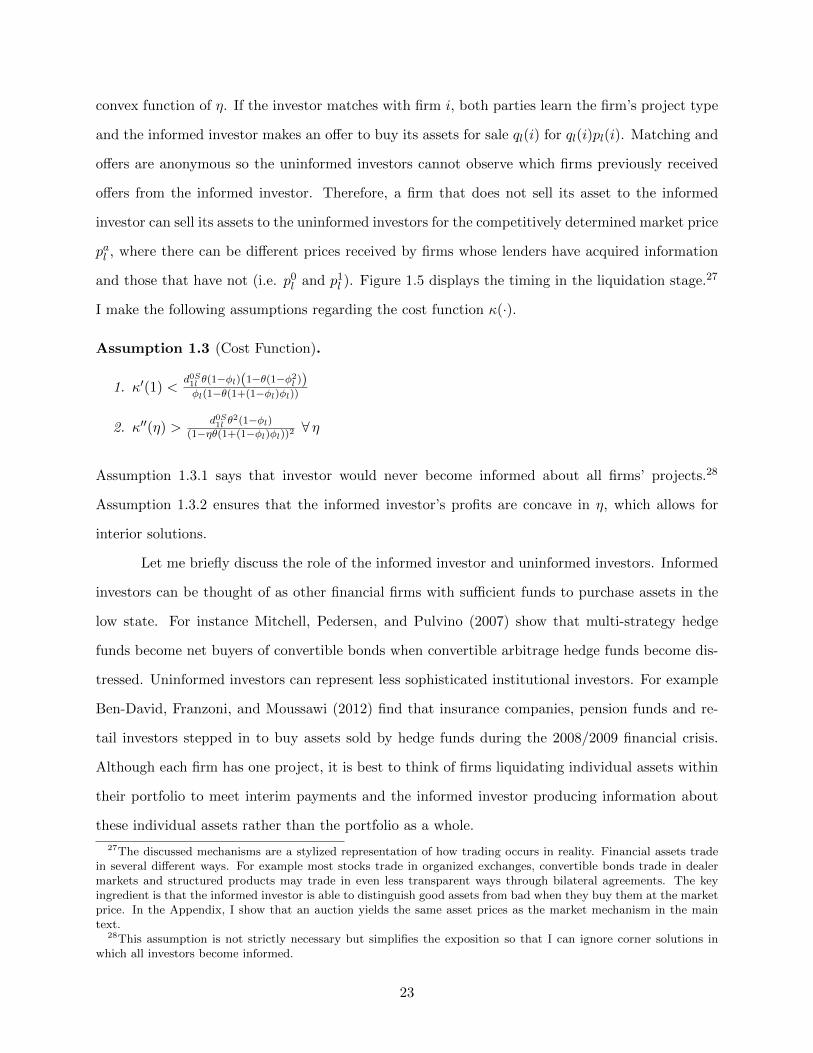
convex function of η. If the investor matches with firm i, both parties learn the firm’s project type
and the informed investor makes an offer to buy its assets for sale ql(i) for ql(i)pl(i). Matching and
offers are anonymous so the uninformed investors cannot observe which firms previously received
offers from the informed investor. Therefore, a firm that does not sell its asset to the informed
investor can sell its assets to the uninformed investors for the competitively determined market price
pal , where there can be different prices received by firms whose lenders have acquired information
and those that have not (i.e. p0l and p1
l ). Figure 1.5 displays the timing in the liquidation stage.27
I make the following assumptions regarding the cost function κ(·).
Assumption 1.3 (Cost Function).
1. κ′(1) <d0S
1l θ(1−φl)(1−θ(1−φ2l ))
φl(1−θ(1+(1−φl)φl))
2. κ′′(η) >d0S
1l θ2(1−φl)
(1−ηθ(1+(1−φl)φl))2 ∀ η
Assumption 1.3.1 says that investor would never become informed about all firms’ projects.28
Assumption 1.3.2 ensures that the informed investor’s profits are concave in η, which allows for
interior solutions.
Let me briefly discuss the role of the informed investor and uninformed investors. Informed
investors can be thought of as other financial firms with sufficient funds to purchase assets in the
low state. For instance Mitchell, Pedersen, and Pulvino (2007) show that multi-strategy hedge
funds become net buyers of convertible bonds when convertible arbitrage hedge funds become dis-
tressed. Uninformed investors can represent less sophisticated institutional investors. For example
Ben-David, Franzoni, and Moussawi (2012) find that insurance companies, pension funds and re-
tail investors stepped in to buy assets sold by hedge funds during the 2008/2009 financial crisis.
Although each firm has one project, it is best to think of firms liquidating individual assets within
their portfolio to meet interim payments and the informed investor producing information about
these individual assets rather than the portfolio as a whole.
27The discussed mechanisms are a stylized representation of how trading occurs in reality. Financial assets tradein several different ways. For example most stocks trade in organized exchanges, convertible bonds trade in dealermarkets and structured products may trade in even less transparent ways through bilateral agreements. The keyingredient is that the informed investor is able to distinguish good assets from bad when they buy them at the marketprice. In the Appendix, I show that an auction yields the same asset prices as the market mechanism in the maintext.
28This assumption is not strictly necessary but simplifies the exposition so that I can ignore corner solutions inwhich all investors become informed.
23

4. Any unsold assets are sold to uninformed for pal
3. Informed investor make offers to buy firms’ assets
2. Informed investor incurs κ(η) to the quality of η projects
1. State z = l is realized
Figure 1.5: Liquidation Stage Timing at t = 1.
1.4.2 Market Equilibrium Analysis
In this section I characterize equilibrium asset prices, investors’ decisions to become informed and
firms’ financial contracts. In the high state both good and bad projects payoff R with certainty;
hence, there is no potential for adverse selection and p0h = p1
h = R. Consider I0 the set of firms
in which their lenders do not acquire information at t = 0 and I1 the set of firms in which their
lenders do acquire information
I0 ≡ {i : a(i) = 0}, I1 ≡ {i : a(i) = 1}.
Firms i ∈ I1 are financed only if the project is good, implying that the uninformed are willing
to pay p1l = R. Therefore, if the informed investor matches with a firm i ∈ I1 in the low state,
the informed investor offers pl(i) = p1l = R and the firm accepts. If a firm i ∈ I1 does not match
with the informed investor, it sells its assets to the uninformed for p1l = R. Hence, regardless of
matching outcomes all firms i ∈ I1 receive p1l = R.
The remaining price to characterize is p0l . Since the informed investor’s matching and offers
are anonymous, uninformed investors cannot distinguish the quality of individual assets in the pool
sold by firms i ∈ I0. Therefore, p0l ∈ [pR,R] where p0
l depends on the inferred proportion of good
assets sold to the uninformed. Consider a firm i ∈ I0 that matches with the informed investor. If
its project is good its expected payoff R is always greater than p0l . Since each firm’s outside option
is p0l , the informed investor offers pl(i) = p0
l and the firm accepts. In contrast, if the project is
bad its expected payoff is pR which is always less than p0l .
29 Thus, the firm rejects any offer the
29I confirm in equilibrium that the inequality is strict.
24

Table 1.1: Liquidation Costs
a = 1 a = 0
z = h γ1h = 0 γ0
h = 0
z = l γ1l = 0 γ0
l = ηθ(1−φl)(1−ηθ)φl ≥ 0
informed investor makes and sells the asset to the uninformed investors for p0l .
30 A firm that does
not match with the informed investor also sells its assets to the uninformed for p0l . Summarizing,
Lemma 1.3.
1. If the informed investor matches with a firm i ∈ I1 at t = 1 it buys the asset at p1l = R
2. If the informed investor matches with a firm i ∈ I0 at t = 1,
(a) it buys the asset at p0l if the asset is good
(b) it does not buy the asset otherwise.
3. Any assets that go unsold to the informed investor are purchased at pal by the uninformed
investors
Lemma 1.3 implies that the market price received by firms i ∈ I0 is
p0l (η) =
(1− ηθ(1− φl)
(1− ηθ)φl︸ ︷︷ ︸γ0l (Adverse selection)
)φlR,︸︷︷︸
Expected value
(1.13)
where p0l (η) is decreasing in η as a larger portion of low quality assets flow to the uninformed due to
the informed investor “cream skimming” good assets. Table 1.1 summarizes the liquidation costs
in each state borne by firms whose lenders acquire and do not acquire information.
Next, I turn to the informed investor’s decision to produce information taking firms’ con-
30Note that even if the firm does not keep any of the proceeds itself, it would default if pRql(i) < d1l(i) whichmeans it always prefers selling the assets for a higher price.
25

tracts as given. Define the aggregate asset sales and payments made by firms i ∈ I0
Q ≡∫I0
ql(i)di, D ≡∫I0
d1l(i)di.
The expected payoff from the informed investor producing information about η firms is
Π(η) =
∫ η
0
(θQ(R− p0
l (η))︸ ︷︷ ︸
Information rents
dη)− κ(η). (1.14)
If the the informed investor matches with a firm i ∈ I1 it pays p1l = R for ql(i) units of the asset
and earns zero profits. If the informed investor matches with a firm i ∈ I0 there is a θ probability
the firm’s asset is good in which case the investor pays p0l (η) for ql(i) units of the asset that yield
R with certainty where (1.14) integrates over all firms i ∈ I0. From Lemma 1.2, d0∗1l = q0∗
l p0l , so
for convenience (1.14) can be written as
Π(η) =
∫ η
0θD
(R
p0l (η)
− 1
)dη − κ(η). (1.15)
Assumption 1.3.2 ensures that the informed investor never produces information about all
assets and 1.3.2 ensures that (1.15) is concave in η.31 If Π(0) < 0 then the informed investor
does not produce information about any projects η∗ = 0. Otherwise, η∗ solves Π′(η∗) = 0. It
immediately follows that η∗ is increasing in D. Formally,
Lemma 1.4. Shorter aggregate maturities induce the informed investor to produce information
about a larger number of projects, i.e. dη∗
dD ≥ 0, where the inequality is strict when η∗ > 0.
Shorter aggregate maturities in turn affect equilibrium asset prices which can be seen by differen-
tiating p0l (η∗) with respect to D
dp0l (η∗)
dD=∂p0
l
∂η∗dη∗
dD≤ 0. (1.16)
The first term is negative and dη∗
dD is positive, and strictly positive when η∗ > 0, from Lemma 1.4.
In summary when η∗ > 0, as D increases, the informed investor produces information about more
31This can clearly be seen by replacing D with the largest amount of t = 1 aggregate payments in the low stated0S
1l .
26

projects, which causes p0l (η∗) drops. Hence, the informed investor’s information production yields
a downward sloping demand curve in the asset market.
Now that I have established the main properties of the liquidation stage, I can define the
market equilibrium.
Definition 1.2. A market equilibrium consists of contracts C(i) for all i, information acquisition
decisions by each firm’s lender a(i) for all i, a mass of firms η∗ that the informed investor produces
information about at t = 1 when z = l, and asset prices {paz}z=h,l, a=0,1, such that:
1. Firms’ contracts are optimal C(i) = C∗ for all i
2. Lenders information acquisition decisions are optimal given contracts
3. The informed investor’s decision to produce information is optimal given firms’ contracts and
asset prices
4. Asset markets clear in each state.
The following definitions will be useful for characterizing the equilibrium.
Definition 1.3. The long-term contract that yields the highest profits and its corresponding profits
are
CL∗ =
C0L if V 0L ≥ V 1L
C1L otherwise,
and
V L∗ = max{V 0L, V 1L}.
I also define aggregate short-term debt α as the mass of firms that borrow short-term which is
equivalent to the amount of investment funded by short-term contracts since k0S = 1 in the short-
term contract. Formally,
Definition 1.4. Aggregate short-term debt α is
α ≡∫ 1
0I(C(i) = C0S)di.
27

Proposition 1.7. The equilibrium mass of firms using short-term contracts α∗, the mass of firms
the informed investor produces information about η∗ and liquidation costs in the low state γ0∗l borne
by firms i ∈ I0 are one of the following types depending on the parameter values
Type 1: α∗ = 1, η∗ = 0 and γ0∗l = 0
Type 2: α∗ = 1, η∗ > 0 and γ0∗l > 0
Type 3: α∗ ∈ (0, 1), η∗ > 0 and γ0∗l > 0,
where in all equilibrium types a mass 1− α∗ of firms choose CL∗.
In the Type 1 equilibrium all firms use short-term contracts and the informed investor does not
produce information about any firms which results in a liquidation cost of zero in the asset market.
In the Type 2 equilibrium all firms use short-term contracts and a positive mass of investors
become informed, where all firms still find it optimal to use short-term contracts because liquidation
costs are not too high. Finally, in the Type 3 equilibrium, if all firms chose short-term contracts,
liquidation costs would be so high that it would no longer be optimal for any firms to use short-term
contracts. When this is the case, a mass of firms less than 1 choose short-term contracts such that
firms are indifferent between the short-term contract and the long-term contract that yields the
highest profits.
When the long-term contract that deters information is more profitable than the long-term
contract that induces information acquisition CL∗ = C0L, there are infinitely many equilibria such
that all firms’ profits equal V 0L.32 However, D∗ and γ0∗l are the same regardless of the equilibrium.
Therefore, for convenience I focus on the case where firms simply choose between C0S and C0L.
Nonetheless, I characterize the full set of equilibria in the proof of Proposition 1.7.33
To understand the real consequences of the market equilibrium, I define aggregate investment
as the sum of realized investment across firms accounting for i) firms that choose C0L invest less
than 1 and ii) firms that choose C1L are only financed when the project is good which occurs with
probability θ. Formally,
32For example there is also a symmetric equilibrium in which all firms choose d1l > 0 and reduce their investmentk < 1.
33The notion of aggregate short-term debt can potentially vary based on the choice of equilibrium (i.e. the amountof investment funded by contracts with payments at t = 1 in the low state); however, the comparative statics aredirectionally the same across equilibria.
28

Definition 1.5. Aggregate investment K is:
K =
α+ (1− α)I0L if CL∗ = C0L
α+ (1− α)θ otherwise.
Therefore, equilibrium aggregate investment K∗ can be characterized in the follow corollary.
Corollary 1.1. If the equilibrium is Type 1 or Type 2, K∗ = 1, otherwise K∗ < 1.
Hence, if the adverse selection in the asset market is severe enough aggregate investment becomes
impaired through a portion of firms resorting to long-term financing.
1.4.3 The Effect of Uncertainty on Aggregate Short-Term Debt and Investment
In this section I show how an increase in uncertainty can lead to a reduction in aggregate short-
term debt and investment. Recall that the only uncertainty in payoffs across project types occurs
in the low state and from Proposition 1.6, the maturity of the short-term contract is decreasing
in the probability of the low state, i.e. d0S1l is increasing in πl. Hence, in the market equilibrium
whenever α∗ = 1 (i.e. Type 1 or Type 2 equilibrium) an increase in πl leads to an increase in
D∗. In the Type 2 equilibrium, higher aggregate payments at t = 1 in the low state lead to an
increase in the mass of investors that become informed causing γ0l to increase. If πl becomes large
enough the equilibrium can switch from Type 2 to Type 3 where some firms must use long-term
contracts, resulting in a drop in aggregate investment and short-term debt. This is summarized in
the following proposition.34
Proposition 1.8. Aggregate investment K∗ and short-term debt α∗ are decreasing in πl.
Although I have only considered exogenous changes in πl, other changes in parameters that increases
the value of information for lenders lead to an increase in d0S1l which in turn increases adverse
selection in the asset market.
Proposition 1.8 can help explain why short-term funding markets periodically become im-
paired. These episodes are often associated with increases in uncertainty and reduced maturities
of short-term debt (e.g. the 2008/2009 financial crisis).
34This is true even if the NPV of the project (πh + πlφl)R− 1 is held constant while πl varies.
29

1.4.4 Welfare
In this section I ask whether firms’ financing decisions in the market equilibrium are efficient. I do
so by considering a concept of constrained efficiency in which a planner can manipulate the mass of
firms using short-term contracts α to maximize welfare, but cannot directly affect the information
production decisions of lenders and the informed investor. For simplicity, I follow Gromb and
Vayanos (2002) by considering an infinitesimal change in α. Total welfare W (α) is the sum of firm
and the informed investor’s profits
W (α) ≡ αV 0S + (1− α)V L∗ + πlΠ(η∗).
Differentiating W (α) with respect to α
dW (α)
dα= V 0S − V L∗ + α
dV 0S
dα+dΠ(η∗)
dα. (1.17)
The first two terms reflect the difference in profits between firms using short-term contracts and
long-term contacts. In the Type 2 equilibrium this is strictly positive, while in the Type 3 equi-
librium it equals zero because firms are indifferent between short and long-term contracts. The
last two terms reflect the two externalities that individual firms do not take into account when
determining their own maturity structures. The third term is the price impact of firms’ short-
term contracts on asset prices which is negative because the demand curve is downward sloping
from (1.16). Finally, the last term is the impact of firms’ short-term contracts on the informed
investor’s profits, which is positive because shorter aggregate maturities allow the informed investor
to buy more assets at a cheap price. The following proposition characterizes the efficiency of the
equilibrium.
Proposition 1.9 (Inefficient Short-Term Debt). The efficiency of each equilibrium type is as follows
1. The Type 1 equilibrium is always constrained efficient
2. The planner can raise welfare in the Type 2 equilibrium by reducing α below α∗ = 1 when
30

demand curve is sufficiently downward sloping
dp0l (η∗)
dα∗< −
p0l (η∗)(d0S
1l Rη∗θ + (V 0S − V L∗ − d0S
1l η∗θ)p0
l (η∗))
d0S1l Rα
∗ (φl − η∗θ).
3. The planner can raise welfare in the Type 3 equilibrium by reducing α below α∗ < 1 when the
demand curve is sufficiently downward sloping
dp0l (η∗)
dα∗< −
η∗θ(R− p0l (η∗))p0
l (η∗)
α∗R (φl − η∗θ),
and raise welfare by increasing α above α∗ < 1 otherwise.
In the Type 1 equilibrium there is no information production at any point and the first-best is
achieved W (α∗) = V FB. However, the Type 2 and Type 3 equilibrium are inefficient if the demand
curve is sufficiently downward sloping. Intuitively, the demand curve slopes downward because
shorter aggregate maturities induce information production in the asset market, which is purely
wasteful from a social perspective. Hence, the planner would like to avoid this if possible. However,
fixing the amount of information the informed investor produces, higher levels of short-term debt
also lead to higher profits from more firms facing an adverse selection discount. While individual
firms would like to avoid the adverse selection discount, it is irrelevant to the planner because it has
no effect on total welfare. The relative magnitude of these two effects determines the efficiency of
the Type 2 and Type 3 equilibrium. In the Type 2 equilibrium there can only be too much short-
term debt since all firms are using short-term contracts (α∗ = 1), while in the Type 3 equilibrium
there can be too little short-term debt when the demand curve sufficiently flat.
Proposition 1.9 can rationalize taxes of short-term debt (i.e. repo contracts or margin loans)
in good times (Type 2 equilibrium) and subsidizing short-term debt when short-term debt markets
become impaired (Type 3 equilibrium). In practice, the latter situation may occur in periods when
adverse selection is already severe and the cost of producing information about marginal projects is
high or informed investors have already devoted substantial capital to investing in distressed assets.
A caveat to my normative analysis is that I have only considered the inefficiency that may
arise from short-term debt through pecuniary externalities in asset markets. There may also be
coordination problems that arise between creditors (e.g. He and Xiong (2012) and Brunnermeier
31

and Oehmke (2013)). In addition, when regulating debt maturity and choosing monetary policy,
policymakers must distinguish between short-term debt demanded by investors with liquidity needs
(e.g. Diamond and Dybvig (1983), Stein (2012) and Diamond (2016)) and short-term debt being
used to prevent inefficient information production by lenders. In Stein (2012), the government can
reduce the incentives of financial institutions to issue safe securities by issuing them itself. This
policy would not have an effect in the context of my model because firms borrow short-term for
reasons unrelated to the demand for safe assets.
In practice, regulators can also directly intervene in asset markets. For example if the a
regulator committed to buying all assets at t = 1 in the low state at R, there would be no incentive
for investors to become informed and the first-best would be achieved. However, asset market
interventions may have other costs such as moral hazard (e.g. Farhi and Tirole (2012a) and Lee
and Neuhann (2017)) or direct costs of intervention. Therefore, I leave the consideration of these
types of interventions for future work.
1.5 Conclusion
In this paper, I propose a new rationale for the widespread use of short-term debt by non-bank
financial firms. In particular, I argue that short-term financing allows financial firms to avoid
excessive information production by their financiers. This problem may be particularly severe for
financial firms that borrow heavily from financial institutions, such as banks, that have expertise
in the same types of assets.
Although short-term financing deters information production at origination, it leads to ex-
cessive information production when firms liquidate to repay their initial lenders following a negative
shock. This delay in information production endogenously raises the cost of short-term financing
through information-based fire sales. Moreover, when market conditions deteriorate, short-term
funding markets can become impaired, i.e. short-term debt maturities shorten, while the volume of
total credit decreases. These implications are consistent with the behavior of numerous short-term
debt markets in the 2008/2009 financial crisis.
From a welfare perspective, my analysis rationalizes 1) policymakers’ concerns that financial
firms’ are overly reliant on short-term debt as opposed to detailed credit analysis (Basel Commit-
32

tee on Banking Supervision (1999)) in normal times and 2) short-term debt markets should be
supported when they malfunction in financial crises.
Future empirical work could directly test whether shorter debt maturities reduce information
production by lenders, while inducing information production in the asset market. In addition,
testing how sensitive asset prices are to short-term debt through deferring information production
may be useful for policymakers in determining whether or not short-term funding markets should
be curbed or supported.
33

1.6 Appendix
1.6.1 Data Description for Figure 1.1
The hedge fund data is from SEC (2019a) where short-term debt is defined as debt with a maturity
under 365 days (Table 48) and Debt/Assets is derived from Borrowing/NAV (Figure 4a). The
mortgage REIT data is from Pellerin, Sabol, and Walter (2013a) where short-term debt is defined
as repo agreements. The mortgage originator debt maturity data comes from Kim et al. (2018)
where they define short-term debt as warehouse loans (typically under a year maturity) and “other
forms of short-term”. Mortgage originator leverage is defined as secured debt to tangible assets and
is taken from a poll of 10 firms by Moody’s (Moody’s Investor Service, 2016). Industrial firms are
from Compustat fiscal year-end 2018 and short-term debt is defined as debt with maturity under
one year. I remove any financial firms within the SIC range of 6000-6999 and exclude firms with
leverage greater than 1.
34

1.6.2 Proofs
Proof of Proposition 1.1. Denote CFB ≡ {kFB, qFBh , qFBl , dFB1h , dFB1l , d
FB2h , d
FB2l } the optimal bench-
mark contract. To show qFBh = 0, suppose to the contrary that qFBh > 0. First suppose that
dFB1h = 0. If the firm reduces qFBh by any ε > 0 where qFBh − ε ≥ 0, (1.4) and (1.5) would not be
violated while the firm’s profits (1.2) would increase because γ0h ≥ 0, which contradicts that CFB
is optimal. Next suppose that dFB1h > 0. If the firm reduces qFBh by any ε > 0 where qFBh − ε ≥ 0,
decreases dFB1h by εp0h
and increase dFB2h by ε, (1.4) and (1.5) would not be violated and (1.2) would
increase. The same steps can be used to show that qFBl = 0. Since qFBh = qFBl = 0, (1.5) implies
that dFB1h = dFB1l = 0.
To show that kFB = 1, suppose to the contrary kFB < 1. If the firm increases kFB by any
ε > 0 where kFB + ε ≤ 1, increases dFB2h by εR and increases dFB2l by 1−πhRπlφl
, (1.4) and (1.5) would
not be violated and the firm’s profits (1.2) would increase. Therefore kFB = 1. We can rewrite the
problem as follows
maxC
∑z
πzφz(R− d2h),
s.t.
1 ≤∑z
πzφzd2z, (1.18)
d2z ∈ [0, R] z = h, l. (1.19)
Since the firm has all of the bargaining power (1.18) binds with equality. Thus any contract that
leads (1.18) to bind and satisfies (1.19) constitutes an optimal benchmark contract and the firm
earns profits
V FB = (πh + πlφl)R− 1.
�
Proof of Lemma 1.1. From (1.8) the lender would produce information if offered CFB. The
firm’s profits would be
θ
(∑z
πz(R− d2z)
). (1.20)
Note that the benchmark optimal contract that makes (1.20) largest while satisfying (1.18) is
d2h = R and d2l = 1−πhRπlφl
which yields
θ (πhR+ πlφlR− 1)
φl. (1.21)
However, (1.21) is strictly less than V FB because θφl< 1 . �
35

Proof of Lemma 1.2. Denote C0∗ ≡ {k0∗, q0∗h , q
0∗l , d
0∗1h, d
0∗1l , d
0∗2h, d
0∗2l } the optimal contract that
deters information acquisition. The same steps from the proof of Proposition 1.1 can be used to
show that q0∗h = d0∗
1h = 0. To show that d0∗1l = q0∗
l p0l , suppose to the contrary q0∗
l p0l > d0∗
1l . If the
firm reduces q0∗l by an ε > 0 where (q0∗
l − ε)p0l ≥ d0∗
1l , (1.5) would not be violated while the firm’s
profits (1.2) would increase because γ0l ≥ 0. Therefore d0∗
1l = q0∗l p
0l . The problem can then be
rewritten as
maxC
πh(kR− d2h) + πlφl
((k − d1l
p0l
)R− d2l
),
s.t.
k ≤ 1,
k ≤ πhd2h + πl(d1l + φld2l), (1.22)
(1− θ)(k − πhd2h − πl(d1l + µd2l)) ≤ c, (1.23)
d2h ≤ kR, (1.24)
d2l ≤(k − d1l
p0l
)R. (1.25)
Next we can prove the incentive compatibility constraint (1.23) binds. By Lemma 1.1, (1.23) is
violated if the following three conditions are true: i) d1l = 0, ii) k = 1 and iii) the participation
constraint (1.22) binds; hence at least one of the above conditions do not hold. I then prove by
contradiction that (1.23) binds in each of these three cases.
Case 1. d0∗1l > 0
Suppose to the contrary that d0∗1l > 0 and (1.23) is slack. There exists a small enough ε > 0 such
that if the firm decreases d0∗1l by ε and increases d0∗
2l by εφl
, then (1.22), (1.23) and (1.25) would not
be violated. This would reduce q0∗l which causes the firm’s profits to increase because γ0
l ≥ 0.
Case 2. k0∗ < 1
Suppose to the contrary that k0∗ < 1 and (1.23) is slack. There exists a small enough ε > 0 such
that if the firm increases k0∗ by ε and increases d0∗2h by εR and increases d0∗
2l by 1−πhRπlφl
, then (1.22),
(1.23), (1.24) and (1.25) would not be violated, while the firm’s profits would increase.
Case 3. The participation constraint (1.22) is slack
Suppose to the contrary (1.22) and (1.23) are slack. There exists a small enough ε > 0 such that if
the firm decreased d0∗2h, d0∗
1l , or d0∗2l by ε, then (1.22), (1.23), (1.24) and (1.25) would not be violated,
while the firm’s profits would increase. These three cases imply that the incentive compatibility
constraint must bind.
Finally to prove d0∗2h = k0∗R, suppose to the contrary d0∗
2h < k0∗R. If the firm increases d0∗2h
by ε > 0 where d0∗2h + ε ≤ k0∗R and decreases d0∗
2l by εφl
, then (1.22), (1.24) and (1.25) would not
36

be violated and (1.23) would slacken. However, as just shown (1.23) must bind at the optimum,
which contradicts C0∗ being optimal. �
Proof of Proposition 1.2. Following Lemma 1.2 and ignoring (1.25) for now, the problem can
be written as
maxC
πlφl
[(k − d1l
p0l
)R− d2l
],
s.t.
k ≤ 1, (1.26)
k(1− πhR) ≤ πl(d1l + φld2l), (1.27)
(1− θ) [k(1− πhR)− πl(d1l + µd2l)] = c. (1.28)
The Lagrangian is
L = πlφl
[(k − d1l
p0l
)R− d2l
]− λ1
[k(1− πhR)− πl(d1l + φld2l)
]−
λ2
[(1− θ) (k(1− πhR)− πl(d1l + µd2l))− c
]− λ3(k − 1).
The Kuhn-Tucker necessary conditions are
Ld1l=πl(p0l (λ1 + (1− θ)λ2)− φlR
)p0l
≤ 0,
Ld2l= πl
[φl (1− λ1)− µ(1− θ)λ2
]≤ 0,
Lk = πlφlR− (1− πhR)(λ1 + (1− θ)λ2)− λ3 ≤ 0,
Ld1ld1l = 0, Ld2l
d2l = 0, Lkk = 0,
λ1
[k(1− πhR)− πl(d1l + φld2l)
]= 0,
(1− θ)[k(1− πhR)− πl(d1l + µd2l)
]− c = 0,
λ3(k − 1) = 0,
λ1 ≥ 0, λ2 > 0, λ3 ≥ 0,
(1.27), (1.28), (1.26).
There are many potential solutions to the system of equations; however, several can be eliminated
immediately upon inspection. After doing so we are left with three potential solutions
k = 1, d1l =1− πhR− cφl
θ(1−φl)
πl, d2l =
c
(1− φl)θπl, (1.29)
λ1 =φl(p
0l − µR)
(1− µ)θp0l
, λ2 =φl(φlR− p0
l )
(1− φl)θp0l
, λ3 =φlR
[πlp
0l − (1− πhR)
]p0l
.
37

k =φlc
(1− φl)θ(1− πhR), d1l = 0, d2l =
c
(1− φl)θπl, (1.30)
λ1 =φl(1− πhR− πlµR)
(1− µ)θ(1− πhR), λ2 =
φl(πhR+ πlφlR− 1)
(1− φl)θ(1− πhR), λ3 = 0.
k = 1, d1l = 0, d2l =1− c− θ − πhR(1− θ)
µ(1− θ)πl, (1.31)
λ1 = 0, λ2 =φl
(1− θ)µ, λ3 =
φl(πhR+ πlµR− 1)
µ.
First, (1.31) can be ruled out because λ3 < 0 from Assumption 1.1.1. In order for (1.29) to be a
solution, it must be the case that γ0l ≤ 1 − 1−πhR
πlφlRso that λ3 ≥ 0. (1.30) is a potential solution
because λ1 > 0 by Assumption 1.1.1. However, Ld1l> 0, only if γ0
l > 1 − 1−πhRπlφlR
. Therefore, if
γ0l ≤ 1− 1−πhR
πlφlR(1.29) is the solution while (1.30) is the solution otherwise. Also, note that (1.25)
is not violated in any of the candidate solutions. �
Proof of Proposition 1.3. Denote C1∗ ≡ {k1∗, q1∗h , q
1∗l , d
1∗1h, d
1∗1l , d
1∗2h, d
1∗2l } the optimal contract
that induces information acquisition. The same steps from the proof of Proposition 1.1 can be
used to show there are no liquidations or payments at t = 1 and k1∗ = 1; however, in all cases
(1.11) must remain slack which is always true because of Assumption 1.2. We can then rewrite the
problem as follows
maxC
θ∑z
πz(R− d2z), (1.32)
s.t.
θ
(∑z
πzd2z − 1
)≥ c, (1.33)
d2z ∈ [0, R] z = h, l. (1.34)
Since the firm has all of the bargaining power (1.33) binds. Therefore any contract that leads (1.33)
to bind and satisfies (1.34) constitutes an optimal contract. The expected profits can be found by
plugging the terms of C1∗ into (1.32). �
Proof of Proposition 1.4. The proof comes immediately from comparing the profits from C0∗
and C1∗ from Propositions 1.2 and 1.3.
�
Proof of Proposition 1.5. Differentiating V 0S with respect to γ0l we have
cφlθ(1−φl) + πhR− 1
(1− γ0l )2
< 0.
38

V 0L and V 1L do not vary with γ0l , hence the lower γ0
l the more likely C∗ = C0S . �
Proof of Proposition 1.6. Differentiating d0S1l with respect to πl we have
R− 1 + cφlθ(1−φl)
π2l
> 0.
Notice this also true if we define maturity asd0S
1l
d0S1l +d0S
2l
∂(
d0S1l
d0S1l +d0S
2l
)∂πl
=cθR
(1− φl) (c+ θ (1− πhR))2 > 0.
�
Proof of Lemma 1.3. See text. �
Proof of Lemma 1.4. To see the effect of shorter maturities on the equilibrium number of in-
formed investors we can apply the implicit function theorem
dη∗
dD=
0 if Π(0) < 0
−∂Π(η∗)∂η∗
Π(η∗)∂D
=θ(1−φl)(1−ηθ−ηθ(1−φl)φl)(1−ηθ+ηθφ2
l )φl((1−ηθ−ηθ(1−φl)φl)2κ′′(η)−Dθ2(1−φl))
if Π(0) ≥ 0,(1.35)
Focusing on −∂Π(η∗)∂η∗
Π(η∗)∂D
, the numerator is always positive and the denominator is positive from As-
sumption 1.3.2. Hence dη∗
dD ≥ 0 and the inequality is strict when Π(0) > 0. �
Proof of Proposition 1.7. For convenience, define the set of contracts that deter the lender from
producing information.
C0 ≡ {C : a = 0}.
Let V 0S(D) denote the profits from the short-term contract and Π(η,D) the informed investor’s
profits each as a function of the aggregate payments at t = 1 in the low state D. I break the proof
into three cases.
Case 1. Π(0, d0S
1l
)< 0
If α = 1 no investors would find it optimal to become informed η = 0. Hence, η∗ = 0, γ0∗l = 0 and
α∗ = 1 (from Proposition 1.4).
Case 2. Π(0, d0S
1l
)≥ 0 and V 0S(d0S
1l ) ≥ V L∗
Since Π(0, d0S
1l
), if α = 1 then a positive mass of investors η∗ > 0 would find it optimal to become
informed resulting in a positive liquidation cost γ0∗l > 0. However, the resulting profits from the
39

short-term contract V 0S(d0S1l ) are sufficiently high enough such that all firms still find it optimal to
choose C0S by Proposition 1.4. Hence α∗ = 1, η∗ > 0, and γ0∗l > 0.
Case 3. V 0S(d0S1l ) < V L∗
If α = 1, the liqudation cost γ0l would be so high that no firms would find it optimal to choose
C0S . However, if α = 0, then γ0l = 0 and all firms would find it optimal to choose C0S . Thus, all
firms must choose contracts C(i) such that they are indifferent between C(i) and the most profitable
long-term contract V (i) = V L∗ for all i.
Lemma 1.5. In Case 3 V (i) = V L∗ for all i.
Proof. Suppose to the contrary there is some contract C′ used in equilibrium in which V ′ 6= V L∗.
First it can never be the case that V ′ < V L∗ by Proposition 1.4. Now suppose that V ′ > V L∗. Since,
C1L = C1∗, if V ′ > V L∗ then C′ ∈ C0. Since V ′ > V 0L it must be that C′ = C0S by Proposition 1.2.
However, if V 0S > V L∗, then all firms would choose C(i) = C0S , which is a contradiction because
V 0S(d0S1l ) < V L∗. Therefore, V (i) = V L∗ for all i in Case 3. �
There are two sub-cases within Case 3.
Subcase 1. CL∗ = C1L
First note that it cannot be that C(i) = C1L for all i because if this were true γ0l = 0 which would
induce all firms to choose C0S . Therefore there must be some contract C′ ∈ C0 used in equilibrium
with profits V ′ where from Lemma 1.5, V ′ = V 1L. From Proposition 1.2, it must be the case that
C′ = C0S . Thus, the only contracts that are used in equilibrium are C0S and C1L where α is the
fraction of firms that choose C0S . Hence, the following equation characterizes α∗
G(α∗d0S1l ) = V 0S
(α∗d0S
1l
)− V 1L = 0.
First note that α∗ 6= 1 because V 0S(d0S1l ) < V 1L. Define α as the largest α such that no investors
become informed η∗ = 0
α = arg maxα
α s.t. η∗ = 0.
Since V 0S(αd0S
1l
)= V FB > V 1L, it must be that α∗ ∈ (α, 1). In this region γ0
l is strictly increasing
in α from (1.35). Hence, V 0S(αd0S
1l
)is strictly decreasing in α and there exists a unique α∗ ∈ (0, 1)
such that G(α∗d0S1l ) = 0.
Subcase 2. CL∗ = C0L
From Lemma 1.5 V (i) = V 0L for all i. It will be useful to establish the following lemma
Lemma 1.6. In Case 3 when CL∗ = C0L, V 0S(D∗) = V 0L.
40

Proof. Suppose V 0S(D∗) < V 0L then from Proposition 1.2 all firms to choose C∗ = C0L. However,
if this is the case γ0l = 0 which is a contradiction. Suppose V 0S(D∗) > V 0L then from Proposition
1.2 all firms would choose C∗ = C0L. However, if this is the case V 0S(d0S1l ) < V 0L which is also a
contradiction. �
Lemma 1.6 implies that the Lagrange multiplier (λ3) on the constraint k ≤ 1 for the candidate
solution (1.29) equals zero. Hence, there can potentially be other contracts C ∈ C0 other than C0S
and C0L used in equilibrium. The following conditions characterize the equilibrium
k(i)(1− πhR) = πl (d1l(i) + φld2l(i)) ∀i,
(1− θ)[k(i)(1− πhR)− πl (d1l(i) + µd2l(i))
]= c ∀i,
d1l(i) ≥ 0 ∀i,
V (i;D∗) = V 0L ∀i.
Each firm’s participation constraint and incentive compatibility constraint bind and all firms must
earn profits equal to the long-term contract with reduced investment given D∗. Further simplifying,
d2l(i) =c
θπl(1− φl)∀i,
k(i) =cφl + d1l(i)(1− φl)θπl
(1− φl)θ(1− πhR)∀i, (1.36)
d1l(i) ≥ 0 ∀i,
V (i;D∗) = V 0L ∀i.
Integrating (1.36) over i,
K∗ =
∫ 1
0k(i)di =
cφl +D∗(1− φl)θπl(1− φl)θ(1− πhR)
.
Since K∗ and D∗ do not depend on the exact distribution of firms’ contracts, I focus on the
case where firms choose between C0S and C0L. Therefore, the following equation characterizes the
equilibrium
G(α∗d0S1l ) = V 0S
(α∗d0S
1l
)− V 0L = 0.
As in the previous sub-case, V 0S(αd0S
1l
)is strictly decreasing in α when α ∈ [α, 1]. Therefore, there
exists a unique α∗ ∈ (0, 1) such that G(α∗d0S1l ) = 0. �
Proof of Corollary 1.1. From Proposition 1.7 in the Type 1 and 2 equilibria α∗ = 1. Therefore
K∗ = 1 because k0S = 1. In the Type 3 equilibrium α∗ < 1 which implies K∗ < 1 because θ < 1
and k0L < 1. �
41

Proof of Proposition 1.8. Recall in the Type 3 equilibrium, α∗ solves
G(α∗d0S1l ) = V 0S
(α∗d0S
1l
)− V L∗ = 0.
Applying the implicit function theorem
dα∗
dπl= −
∂G∂πl
∂G∂η∗
dη∗
dD∂D∂α∗
= − (−)
(−)(+)(+)< 0. (1.37)
Differentiating K∗ with respect to πl when CL∗ = C0L
dK∗
dπl
∣∣∣CL∗=C0L
= (1− α∗) ∂k0L
∂πl︸ ︷︷ ︸(−)
+(1− k0L)dα∗
dπl︸︷︷︸(−)
< 0.
and when CL∗ = C1L
dK∗
dπl
∣∣∣CL∗=C1L
= (1− θ) dα∗
dπl︸︷︷︸(−)
< 0.
Next we need to show that K∗ is decreasing in πl at the point where V 0L = V 1L. First note that
V 0L − V 1L is decreasing in πl
∂(V 0L − V 1L)
∂πl= −
c(R− 1)Rφ2l
(1− φl)θ(1− πhR)2< 0.
This implies that as πl increases it becomes more likely that CL∗ = C1L. Finally we need to show
that the realized investment level for C1L is lower than C0L when the profits from those contracts
are equal i.e. θ < k0L when V 1L = V 0L
k0L − θ =cφl
θ(1− φl)(1− πhR)− θ,
which is negative when V 1L = V 0L. Hence, when the equilibrium is Type 3, both K∗ and α∗ are
decreasing in πl. The last step is to show that as πl increases the equilibrium moves from Type 1
to Type 2 to Type 3. When the equilibrium is Type 1 the following condition holds
Π(0, d0S
1l
)< 0. (1.38)
Since d0S1l is increasing in πl, an increase in πl tightens (1.38). When the equilibrium is Type 2, the
42

following conditions are true
Π(0, d0S
1l
)> 0, (1.39)
V 0S(d0S
1l
)≥ V L∗ (1.40)
An increase in πl relaxes (1.39) and from (1.37) tightens (1.40). Therefore, as πl increases the
equilibrium moves from Type 1 to Type 2. When the equilibrium is Type 3, the following condition
is true:
V 0S(d0S
1l
)< V L∗. (1.41)
An increase in πl relaxes (1.41). Therefore, as πl increases the equilibrium moves from Type
2 to Type 3. Note that the equilibrium cannot jump from Type 1 to Type 3 from increasing πl
continuously because (1.38) implies (1.40). Summarizing, if an increase in πl causes the equilibrium
to switch types, the new equilibrium type results in a lower K∗ and α∗. Together all of these pieces
imply that α∗ and K∗ are decreasing in πl. �
Proof of Proposition 1.9 . In the Type 1 equilibrium, there is no information production by
lenders or the informed investor and all firms fully invest K∗ = 1. Hence the Type 1 equilibrium
achieves the first-best: V 0S = V FB. In the Type 2 equilibrium η∗ > 0 and α∗ = 1. Since all firms
choose the short-term contract there can never be too little short-term financing.
From the terms in (1.17) first notice that
dV 0S
dα∗=d0S
1l Rα∗φl
dp0l (η∗)
dα∗
p0l (η∗)2
. (1.42)
Also notice that
dΠ(η)
dα∗=
d
dα∗
∫ η∗
0θD
(R
p0l (η∗)− 1
)dη − κ(η∗)
=
[θD
(R
p0l (η∗)− 1
)]dη∗
dα∗η∗ +
∂
∂η∗dη∗
dα∗
∫ η∗
0
[θD
(R
p0l (η∗)− 1
)]dη − κ(η∗)
=
[θD
(R
p0l (η∗)− 1
)]dη∗
dα∗η∗
=d0S
1l η∗θ(R(p0l (η∗)− α∗ dp
0l (η∗)
dα∗
)− p0
l (η∗)2)
p0l (η∗)2
(1.43)
where the third line comes from the fact that∫ η∗
0ddα
[θD(
Rp0l (η∗)− 1)]dη − d
dακ(η∗) = 0 at the
informed investor’s optimal information production choice. Substituting (1.42) and (1.43) into
43

(1.17) we have
dW (α)
dα= V 0S − V L∗ + d0S
1l
(Rη∗θp0
l (η∗) +Rα (φl − η∗θ)
dp0l (η∗)
dα∗
p0l (η∗)2
− η∗θ
)
Simplifying in terms ofdp0l (η∗)
dα∗ we have the following condition for dV 0S
dα∗ < 0 in the Type 2 equilibrium
dp0l (η∗)
dα∗<p0l (η∗)(d0S
1l Rη∗θ + (V 0S − V L∗ − d0S
1l η∗θ)p0
l (η∗))
d0S1l Rα
∗ (φl − η∗θ). (1.44)
Hence, whenever the demand curve is sufficiently downward sloping there is too much short-term
financing in the Type 2 equilibrium. In the Type 3 equilibrium α∗ < 1, hence there can potentially
be too much or too little short-term financing. At the Type 3 equilibrium point V 0S − V L∗ = 0 so
(1.44) simplifies to
dp0l (η∗)
dα∗< −
η∗θ(R− p0l (η∗))p0
l (η∗)
α∗R (φl − η∗θ),
Hence whenever the demand curve is sufficiently downward sloping, the planner can raise welfare by
reducing the amount of short-term financing. Otherwise, the planner can raise welfare by increasing
the amount of short-term financing. �
44

1.6.3 Firm Can Raise Additional Funds at t = 0 and Store Funds Across Dates
In the main text I do not allow the firm to raise additional funds beyond k at t = 0 or store funds
across dates. In this section I show that this is without loss of generality. Consider the following
revised definition of a financial contract.
C ≡ {k, qz, d0, d1z, d2z(R), e0, e1z, e2z(R)}z=h,l, R=R,0 (1.45)
The differences between Definition 1.1 and (1.45) are i) d0 which is the funds the firm raises at
t = 0 which can potentially exceed k and ii) the payment at t = 2 d2z(R) can be conditioned on the
project’s success or failure, and iii) e is the firm’s consumption that may depend on the state and
project output. The revised definition of the contract will only be relevant for the optimal contract
without information acquisition C0∗. For the optimal contract with information production C1∗ as
long as the firm captures the full surplus and the lender acquires information its profits will always
be V 1∗ = θ(R − 1) − c. The timing of the firm’s consumption is irrelevant because the firm is
risk-neutral and there is no discounting. Hence, it is without loss of generality to assume the firm
stores any excess funds raised at t = 0 to t = 1. The firm’s problem can be written as
maxC
d0 − k +∑z
πz
[qzp
0z − d1z + φz [(k − qz)R− d2z(R)]− (1− φz)d2z(0)
],
s.t.
k ≤ d0, k ≤ 1,
d0 ≤ πh(d1h + d2h) + πl [d1l + φld2l(R) + (1− φl)d2l(0)] ,
(1− θ) (d0 − πh(d1h + d2h)− πl [d1l + pd2l(R) + (1− p)d2l(0)]) ≤ c, (1.46)
qz ∈ [0, k], d1z ≤ qzp0z + d0 − k z = h, l,
d2h(R) ≤ d0 − k + qhp0h − d1h + (k − qh)R,
d2l(R) ≤ d0 − k + qlp0l − d1l + (k − ql) R R = R, 0,
p0z = (1− γ0
z )φzR, z = h, l.
Using the same steps from Proposition 1.1 we can show q0∗h = 0. Since there is no difference in the
lender’s expected payments or the firm’s profits if the lender receives payments in the high state
at t = 1 or t = 2 it is w.l.o.g to set d0∗h = 0. In addition, using the same steps from Lemma 1.2 we
can show the incentive compatibility constraint (1.46) binds and d0∗2h = k0∗(R− 1) + d0∗
0 . Define δ1
as the firm’s cash at the beginning of t = 1
δ1 ≡ d0 − k,
and δ2z as the firm’s cash at the beginning of t = 2:
δ2z ≡ d0 − k + qzp0z − d1z z = h, l.
45

We can then rewrite the problem as follows
maxC
πl
[φl [δ2l + (k − ql)R− d2l(R)] + (1− φl) [δ2l − d2l(0)]
], (1.47)
s.t.
k ≤ d0, k ≤ 1,
d0 ≤ πh(δ1 + kR) + πl [d1l + φld2l(R) + (1− φl)d2l(0)] , (1.48)
(1− θ) (d0 − πh(δ1 + kR)− πl [d1l + µd2l(R) + (1− µ)d2l(0)]) = c, (1.49)
ql ∈ [0, k], d1l ≤ qlp0l + δ1
d2l(R) ≤ δ2l + (k − ql) R R = R, 0,
p0z = (1− γ0
z )φzR, z = h, l.
It will be useful to establish the following lemma.
Lemma 1.7. d2l(0)0∗ = δ0∗2l
Proof. Suppose to the contrary d2l(0)0∗ < δ0∗2l . First consider the case in which d0∗
2l (R) > 0. If the
firm increases d2l(0)0∗ by ε > 0 where d2l(0)0∗ + ε ≤ δ0∗2l and reduces d0∗
2l (R) by(
1−φlφl
)ε, (1.48)
would not be violated while (1.49) would slacken which contradicts C0∗ being optimal. Next consider
the case in which d0∗2l (R) = 0. Since πhR < 1, it must be that q0∗
l > 0 in order for (1.48) to not be
violated. To see this, suppose that q0∗l = 0, and insert the largest value of d2l(0)0∗ = d0 − k − d1l
into (1.48) and we have
k(1− πhR)− πlφl(d0 − k − d1l) ≤ 0 (1.50)
Inserting the largest possible value of d0∗1l = d0 − k into (1.50) we have
k(1− πhR) ≤ 0
Which is violated so long as k > 0. Hence q0∗l > 0. The firm can then reduce q0∗
l by ε and no
constraints are violated while the firm’s profits (1.47) increase since γ0l ≥ 0. �
46

Once again rewriting the problem following Lemma 1.7
maxC
πlφl [δ2l + (k − ql)R− d2l(R)] ,
s.t.
k ≤ d0, k ≤ 1,
d0 ≤ πh(δ1 + kR) + πl [d1l + φld2l(R) + (1− φl)δ2l] , (1.51)
(1− θ) (d0 − πh(δ1 + kR)− πl [d1l + µd2l(R) + (1− µ)δ2l]) = c, (1.52)
ql ∈ [0, k], d1l ≤ qlp0l + δ1
d2l(R) ≤ δ2l + (k − ql)R,
p0l = (1− γ0
l )φlR.
Expanding (1.51) and (1.52),
d0 ≤ πh(δ1 + kR) + πl[φl(d1l + d2l(R)) + (1− φl)qlp0
l
],
(1− θ)(d0 − πh(δ1 + kR)− πl
[µ(d1l + d2l(R)) + (1− µ)qlp
0l
])= c.
Upon inspection, we can see the lender’s incentives to acquire information and the firm’s profits
are invariant between d1l and d2l(R), i.e. storing funds from t = 1 to t = 2. Hence, it is without
loss of generality to set δ0∗2l = 0 and rewrite the problem as
maxC
πlφl [δ1 + (k − ql)R− d2l(R)] ,
s.t.
k ≤ d0, k ≤ 1,
d0 ≤ πh(δ1 + kR) + πl [d1l + φld2l(R)] ,
(1− θ) (d0 − πh(δ1 + kR)− πl [d1l + µd2l(R)]) = c,
ql ∈ [0, k], d1l ≤ qlp0l + δ1, d2l(R) ≤ (k − ql)R,
p0l = (1− γ0
l )φlR.
We can use the same steps from Lemma 1.2 to show that d0∗1l = q0∗
l p0l + δ0∗
1 . The problem can be
47

written as
maxC
πlφl [(k − ql)R− d2l(R)] ,
s.t.
k ≤ 1,
k ≤ πhkR+ πl(qlp
0l + φld2l(R)
),
(1− θ)(k − πhkR− πl(qlp0
l + µd2l(R)))
= c,
ql ∈ [0, k], d2l(R) ≤ (k − ql)R,
p0l = (1− γ0
l )φlR,
where d0 simply drops out. Hence, it is without loss of generality that the firm only raises k initially
and does not store funds across periods.
1.6.4 Firm Knows Project Type and Lender Cannot Acquire Information
In this section, I analyze the case in which the firm knows υ and the lender cannot acquire infor-
mation. This is useful to show that exogenous asymmetric information alone will not lead to firms’
using short-term financing.
Because the firm knows its project type, its contract offer may be a signal about its type.
First note that there can never be a separating equilibrium because the bad project is NPV negative.
Depending on off-equilibrium beliefs, there can be a multiplicity of equilibria. To narrow down the
potential equilibria, I apply undefeated equilibrium refinement from Mailath, Okuno-Fujiwara, and
Postlewaite (1993).
This refinement allows the firm with the good project to choose a contract that yields the
highest profits subject to being mimicked by the firm with the bad project. The problem can be
written as
maxC
∑z
πz(qzp
0z − d1z + (k − qz)R− d2z
)s.t.
k ≤ 1,
k ≤∑z
πz(d1z + φzd2z), (1.53)
qz ∈ [0, k], d1z ≤ qzp0z, d2z ≤ (k − qz)R z = h, l,
p0z = (1− γz)φzR, z = h, l.
The following lemma immediately follows.
Lemma 1.8. In the optimal contract in which the firm knows its project type and the lender cannot
acquire information,
48

i) q∗h = q∗l = 0
ii) d∗1h = d∗1l = 0
iii) k∗ = 1
iv) d∗2h = R.
Proof. i) and ii) follow from the same steps as Proposition 1.1. Suppose k∗ < 1. If we increase k∗
by ε and increase d∗2h by εR and increase d∗2l by ε(1−πhR)πlφl
(1.53) is not violated and the objective
increase which is a contradiction. Suppose that d∗2h < R. If we increase d∗2h by ε and decrease d∗2lby πhε
πlφl(1.53) is not violated and the objective increase which is a contradiction. �
After Lemma 1.8, the problem reduces to
maxC
πl(R− d2l)
s.t.
(1− πhR) ≤ πlφld2l. (1.54)
Since the firm has all of the bargaining power (1.54) binds and the optimal contract is
C∗ ≡ {k∗, q∗h, q∗l , d∗1h, d∗1l, d∗2h, d∗2l} =
{1, 0, 0, 0, 0, R,
1− πhRπlφl
}.
1.6.5 Firm Knows Project Type and Lender Can Acquire Information
In this section, I analyze the case in which the firm knows υ and the lender has the same information
acquisition technology as in the baseline model. I apply the same undefeated equilibrium refinement
from Mailath, Okuno-Fujiwara, and Postlewaite (1993). Therefore, the firm with the good project
chooses the contract that maximizes its profits subject to pooling with the firm with the bad project.
Note that because the lender can acquire information, the lender may be able to distinguish the
types after the contract offer. Similarly, when the firm knows its type the optimal contract without
information production coincides with the optimal contract from the main text C1∗ = C1L. Since
from Lemma 1.1, the lender will acquire information if the firm offers a contract in which k = 1
and ql = d1l = 0, the firm with the good project’s profits from C1L is
R− 1− c. (1.55)
For simplicity, assume information acquisition is contractible. As in the benchmark case there is
no value to liquidations; therefore, the lender’s break-even condition is
k ≤∑z
πzφzd2z. (1.56)
49

To minimize pooling costs, the firm with the good project chooses d2h = kR and (1.56) binds.
Therefore, the firm with the good project’s profits are
πlk
(R− 1− πhR
πlφl
),
which is strictly less than (1.55). Hence, the firm with the the good project wants to induce the
lender to acquire information to avoid the pooling cost with the firm with the bad project. This
result is similar to Fulghieri and Lukin (2001). Therefore, the optimal contract is C∗ = C1L.
1.6.6 Both Firm and Lender Can Acquire Information
In this section I analyze the case in which the firm can also incur c to learn υ. Before the firm offers
the lender a contract, the firm decides whether to acquire information or not. If the firm produces
information the choice of producing information becomes immediately public, while υ is revealed
at the end of t = 0. I assume the firm’s information production choice becomes public to avoid the
problem of the firm discovering it has a bad project then attempting to pool with a firm that does
not produce information. The rest of the timing is exactly the same as in the baseline model in
Section 1.2.
From Section 1.6.5, the optimal contract conditional on the firm knowing its project type
is C1L. If the firm acquires information then offers C1L, the firm with the good project’s expected
profits will be V 1L−c which is strictly less than V 1L, hence the firm would not acquire information.
Summarizing,
Proposition 1.10. If the firm has access to the same information technology as the lender at the
beginning of t = 0, it does not acquire information and the optimal contract is the same as in the
main text.
1.6.7 Firm Receives Exogenous Information
In the baseline model, the firm and lender begin symmetrically uninformed; however in practice, it
seems plausible firms have some form of information advantage over their lenders. In this section
I show that if the firm receives an exogenous noisy signal regarding its project type the optimal
contract may still deter information production. Suppose that prior to offering the lender a contract
the firm receives a signal s ∈ {G,B} regarding υ. Specifically, s = G with probability 12 and
Pr(υ = g|s = G) = θ + ε and Pr(υ = b|s = B) = θ − ε otherwise where ε ≤ max{θ, 1 − θ}.The change in probability need not be symmetric, but this simplification makes the unconditional
probability of the project succeeding the same as in the baseline model (i.e. Pr(υ = g|s = G)Pr(s =
G) + Pr(υ = g|s = B)Pr(s = B) = θ). The firm’s signal is private information and the lender has
access to the same information acquisition technology in the baseline model. Once again, I use the
undefeated equilibrium refinement from Mailath, Okuno-Fujiwara, and Postlewaite (1993) so the
50

problem amounts to the firm that receives the good signal s = G maximizing its profits subject to
pooling with the firm that receives the bad signal s = B. Define
φh(G) ≡ 1, φl(G) ≡ θ + ε+ (1− θ − ε)µ.
Then the firm that receives signal s = G faces the following problem to deter information production
maxC
∑z
πz
[qzp
0z − d1z + φz(G) ((k − qz)R− d2z)
]s.t.
k ≤ 1,
k ≤∑z
πz(d1z + φzd2z),
(1− θ) [k − πh(d1h + d2h)− πl(d1l + µd2l)] ≤ c,
qz ∈ [0, k], d1z ≤ qzp0z, d2z ≤ (k − qz)R z = h, l,
p0z = (1− γz)φzR, z = h, l.
Proposition 1.11. When the firm receives an exogenous private signal regarding the project type,
the optimal contract that deters information production takes the form C0L or C0S depending on
parameters.
The steps are the same as in the main text so I omit them. For the problem that induces information
acquisition the firm that receives the good signal solves the following problem
maxC
(θ + ε)∑z
πz(qzp
1z − d1z + (k − qz)R− d2z
)s.t.
k ≤ 1,
c ≤ θ
(∑z
πz(d1z + d2z)− k
),
c ≤ (1− θ) [k − πh(d1h + d2h)− πl(d1l + µd2l)] ,
qz ∈ [0, k], d1z ≤ qzp1z, d2z ≤ (k − qz)R z = h, l,
p1z = (1− γ1
z )R z = h, l.
The following proposition immediately follows
Proposition 1.12. When the firm receives an exogenous private signal regarding the project type,
the optimal contract that induces information production takes the form C1L.
51

The firm that receives the good signal’s expected profits from the three classes of contracts are
V 0L(G) = k0L(πhR+ πlφl(G)R− 1),
V 0S(G) = πlφl(G)
(R− d0S
2l −d0S
1l
(1− γ0l )φl
),
V 1L(G) = (θ + ε)(R− 1)− c.
Both V 1L(G) − V 0S(G) and V 1L(G) − V 0S(G) are increasing in ε. Hence, when the firm begins
with private information, it is more likely the optimal contract induces information production.
However, there are still parameter ranges in which the optimal contract is short-term (e.g. when ε
and γ0l are small).
1.6.8 NPV Positive Bad Project
In this section, I characterize the optimal contract when the bad project is NPV positive. Specifi-
cally,
(πh + πlµ)R > 1. (1.57)
Condition (1.57) implies that c < 0, therefore I impose the additional assumption that c > 0, i.e.
c ∈ (0, c). To keep the problem interesting, I also impose the following condition
πhR < 1 (1.58)
Condition (1.58) ensures the lender cannot breakeven by only receiving payments in the high state
where there is no uncertainty across project types. The firm’s problem for the optimal contract
without information acquisition C0∗ remains the same. However, if we inspect the potential solutions
from Proposition (1.2), note that now (1.30) can be ruled out because of (1.57) and (1.31) is the
solution when γ0l ≥
1−πhRπlφlR
and (1.29), C0S , is the solution otherwise.
The optimal contract that induces information acquisition C1∗ can differ from the case in
which the bad project was NPV negative because the firm can offer a menu to induce the lender to
accept different terms depending on υ. I use superscripts to refer to the contract terms intended for
the specific project type. To keep notation manageable, I suppress the references to the optimality
of the contract throughout the proofs. For instance if I state qbl = 0 in a Lemma, this refers to the
value of qbl at the optimum unless otherwise stated. The firm’s problem that induces information
acquisition is
52

maxkυ ,dυ2z
θ[πh((kg − qgh)R− dg2h) + πl((k
g − qgl )R− dg2l)]
+
(1− θ)[πh((kb − qbh)R− db2h) + πlµ((kb − qbl )R− db2l)
],
s.t.
kυ ∈ [0, 1] υ = g, b,
c ≤ θ(∑
z
πz(dg1z + dg2z)− k
g)
+
(1− θ)(πh(db1h + db2h) + πl(d
b1l + µdb2l)− kb
), (1.59)
kg ≤∑z
πz(dg1z + dg2z), (1.60)
kb ≤ πh(db1h + db2h) + πl(db1l + µdb2l), (1.61)∑
z
πz(db1z + db2z)− kb ≤
∑z
πz(dg1z + dg2z)− k
g, (1.62)
πh(dg1h + dg2h) + πl(dg1l + µdg2l)− k
g ≤ πh(db1h + db2h) + πl(db1l + µdb2l)− kb, (1.63)
qυz ∈ [0, kυ], dυ1z ≤ qυz (1− γ1z )E[R|υ, z], dυ2z ≤ kυR z = h, l, υ = g, b,
where (1.59) is the lender’s ex-ante participation constraint, (1.60) and (1.61) are the lender’s
participation constraints conditional on discovering the project is good (bad) and (1.62) says if the
firm discovers the project is good it must be incentive compatible to accept the terms for the good
project and vice versa for (1.63).
Lemma 1.9. qυh = dυ1h = 0, υ = g, b.
Proof. The proof is the same regardless of υ. Suppose that qυh > 0 for any υ ∈ {g, b}. First suppose
that dυ1h = 0, then the first can reduce qυh by ε and no constraints are violated and the firm’s profits
increase because γ1h ≥ 0. Next suppose dυ1h > 0, the firm can decrease qυh by ε, decrease dυ1h by
ε(1−γ1
h)E[R|υ,z=h]and increase dυ2h by ε
(1−γ1h)E[R|υ,z=h]
and none of the constraints are affected and the
firm’s profits increase because γ1h ≥ 0. Hence, qυh = 0 and thereby dυ1h = 0 for all υ. �
To simplify the proof I make the following claim which I confirm is true at the conclusion
of the proof
Claim 1.1. (1.63) is slack.
I then establish the following lemma.
Lemma 1.10. qυl = dυ1l = 0 υ = g, b.
53

Proof. The same steps from Lemma 1.9 can be taken to show that qgl = dg1l = 0. Next, suppose
that qbl > 0. There are two cases to consider. First suppose that db1l = 0, then the first can
reduce qbl by ε and no constraints are violated and the firm’s profits increase because γ1l ≥ 0. Next
suppose db1l > 0, the firm can decrease qbl by ε, decrease db1l by ε(1−γ1
l )E[R|υ=b,z=l]and increase db2l by
εµ(1−γ1
l )E[R|υ,z=l] and (1.62) is relaxed while none of the other constraints are affected and the firm’s
profits increase because γ1l ≥ 0. �
Hence, the contract is long-term and we can rewrite the problem as
maxkυ ,dυ2z
θ[πh(kgR− dg2h) + πl(k
gR− dg2l)]
+
(1− θ)[πh(kbR− db2h) + πlµ(kbR− db2l)
],
s.t.
kυ ∈ [0, 1] υ = g, b,
c ≤ θ(πhdg2h + πldg2l − k
g) + (1− θ)(πhdb2h + πlµdb2l − kb),
kg ≤ πhdg2h + πldg2l,
kb ≤ πhdb2h + πlµdb2l,
πhdb2h + πld
b2l − kb ≤ πhd
g2h + πld
g2l − k
g,
dυ2z ≤ kυR z = h, l, υ = g, b.
Lemma 1.11. (1.60) is slack and kg = 1
Proof. Suppose (1.60) binds, then we can replace kg = πhdg2h + πld
g2l into (1.62) which simplifies
to kb ≥ πhdb2h + πld
b2l; however, this violates (1.61). Suppose kg < 1, then we can increase kg by ε
such that kg + ε ≤ 1 and increase dg2h by πhε and dg2l by πlε and (1.62) and (1.59) are not violated
and the firm’s profits increase.
�
Lemma 1.12. (1.59) is slack if kb = 1
Proof. Suppose to the contrary that (1.59) binds if kb = 1, then we can rewrite (1.62) as
πhdb2h + πlφld
b2l − 1− c
θ≤ 0. (1.64)
For (1.64) to hold, we need πhdb2h + πlφld
b2l to be sufficiently small while not violating (1.60) and
db2z ≤ R for all z ∈ {h, l}. It easily shown that the LHS of (1.64) is smallest when (1.60) binds and
dg2h = R; however, even when this is the case (1.64) is violated. �
54

Lemma 1.13. (1.62) binds.
Proof. Suppose to the contrary (1.62) is slack. First consider the case in which kb < 1, we can
increase kb by ε and increase db2h by ε and db2l by εµ such that remains (1.62) is not violated while
(1.59) remains unchanged and the firm’s profits increase. Now consider the case in which kb = 1.
From Lemma 1.12, (1.59) is slack. Hence we can decrease dg2h by a small enough ε such that (1.59),
(1.60) and (1.62) remain slack while increasing the firm’s profits. �
Lemma 1.14. (1.61) binds
Proof. Suppose to the contrary that (1.61) is slack. First consider the case in which kb = 1. When
this is the case (1.59) is slack from Lemma 1.12. Hence we can decrease db2l (note db2l > 0 because
otherwise (1.61) would be violated) by a small enough ε such that (1.59) is not violated, (1.62)
would not be violated and the firm’s profits would increase. Now consider the case in which kb < 1
if we increase kb by ε and increase dg2l or dg2h by ε θπh(1−θ)µ such that (1.61) remains slack, then (1.59)
remains unchanged and (1.62) slackens while the firm’s profits increase.
�
Lemma 1.15. db2h = kbR
Proof. Suppose to the contrary that db2h < kbR, then we can increase db2h by ε and decrease db2l byπhεπlµ
(db2l must be positive because otherwise (1.59) is violated) such that (1.59) and (1.61) remain
unchanged; however, (1.62) slackens which leads to a contradiction. �
Hence from we can rewrite the problem as
maxkb,dg2h,d
g2l,d
b2l,θ[πh(R− dg2h) + πl(R− dg2l)
]+ (1− θ)πlµ
(kbR− db2l
), (1.65)
s.t.
kb ≤ 1 (1.66)
c ≤ θ(πhdg2h + πldg2l − 1) + (1− θ)(πhkbR+ πlµd
b2l − kb), (1.67)
kb = πhkbR+ πlµd
b2l,
πhkbR+ πld
b2l,−kb = πhd
g2h + πld
g2l − 1, (1.68)
dg2z ≤ kgR z = h, l.
Notice that (1.65), (1.67), (1.68) depend on the expected payments from the good project πhdg2h +
πldg2l, but not the relative values of dg2h and dg2l. Hence, we can set dg2h = R (which will ensure
55

Claim 1.1 holds). The Lagrangian is
L = θ[πh(R− dg2h) + πl(R− dg2l)
]+ (1− θ)πlµ
(kbR− db2l
)− λ1(kb − 1)−
λ2
[c− θ(πhdg2h + πld
g2l − 1)− (1− θ)(πlµdb2l − kb(1− πhR))
]−
λ3(kb(1− πhR)− πlµdb2l)− λ4
(kb(πhR+
1− πhRµ
− 1
)− πhdg2h − πlR+ 1
)−
λ5(dg2l −R)− λ6(db2l − kbR).
The Kuhn-Tucker necessary conditions are
Lkb = πl(1− θ)µR− λ1 − (1− πhR) ((1− θ)λ2 + λ3 − λ4) + λ6R ≤ 0,
Ldb2l = πl [(1− θ)µ (λ2 − 1) + µλ3 − λ4]− λ6 ≤ 0,
Ldg2l = πl (θ (λ2 − 1) + λ4)− λ5 ≤ 0,
Lkbkb = 0, Ldb2ldb2l = 0, Ldg2ld
g2l = 0,
λ1(kb − 1) = 0,
λ2
[c− θ(πhdg2h + πld
g2l − 1)− (1− θ)(πlµdb2l − (1− πhR)kb)
]= 0,
kb(1− πhR)− πlµdb2l = 0,
πhkb(R− dg2h) + kb
(1− πhR
µ− 1
)− πlR+ 1 = 0,
λ1 ≥ 0, λ2 ≥ 0, λ3 > 0, λ4 > 0, λ5 ≥ 0, λ6 ≥ 0,
(1.66), (1.67).
There are two potential solutions
kb =cµ
θ(1− µ)(1− πhR), dg2l =
c+ θ(1− πhR)
θπl, db2l =
c
θπl(1− µ), (1.69)
λ1 = 0, λ2 =(µ+ θ(1− 2µ)) (1− πhR)−R(1− θ)µ2πl
θ(1− µ) (1− πhR),
λ3 =(1− θ)φl (πhR+ πlµR− 1)
θ(1− µ) (1− πhR), λ4 =
(1− θ)µ (πhR+ πlµR− 1)
(1− µ) (1− πhR),
λ5 = 0, λ6 = 0,
56

and,
kb = 1, dg2l =c+ θ(1− πhR)
θπl, db2l =
c
θπl(1− µ), (1.70)
λ1 = πl(1− θ)µR−(µ+ θ(1− 2µ)) (1− πhR)
µ, λ2 = 0,
λ3 = 1 + θ
(1
µ− 1
), λ4 = θ, λ5 = 0, λ6 = 0,
where, (1.69) is the solution when (µ+ θ(1− 2µ)) (1− πhR)− R(1− θ)µ2πl ≥ 0 and (1.70) is the
solution otherwise. We can also now confirm Claim 1.1. When (1.69) is the solution (1.63) reduces
to
µ(
1 +c
θ
)+ πh(1− µ)R− 1 ≤ 0,
which holds. When (1.70) is the solution, the LHS of (1.63) reduces to 0, hence (1.63) holds. The
respective profits for (1.69) and (1.70) are
θ(R− 1)− c+c(1− θ)µ (πhR+ πlµR− 1)
θ(1− µ) (1− πhR), (1.71)
φl (πhR+ µπlR− 1)
µ.
Notice that (1.71) is strictly greater than V 1L. Hence, the optimal contract with information
acquisition is either (1.69) or (1.70). To find C∗ we can simply compare the profits from the
optimal contract with information acquisition and that without information acquisition.
Intuitively, the firm is able to finance the project regardless of its type; however, there is
still a welfare loss relative to the first-best because the lender produces information. Hence, for γ0l
sufficiently close to 0 the optimal contract is short-term C∗ = C0S .
1.6.9 Non-Zero Project Payoff in the Case of Failure
Because the project yields 0 in the case of failure, it is not possible to distinguish between equity
and debt for payments at t = 2. In this section I show that state-contingent debt is the optimal
contract when the project yields a positive payoff in the case of failure. Suppose that R = r < 1
when the project fails. To analyze the interesting case I revise Assumption 1.1 as follows
Assumption 1.4. The bad project is NPV negative:
πhR+ πl(µR+ (1− µ)r) < 1,
while the ex-ante, average project is NPV positive:
πhR+ πl(φlR+ (1− φl)r) > 1,
57

and Assumption 1.2 as follows,
Assumption 1.5. c ∈ (c, c), where
c ≡ (1− θ)(1− πl ((1− µ)r + µR)− πhR),
and
c ≡ θ(1− φl)(1− πhR− πlr)φl
.
Let d2z(r) denote the promised payment from the firm to the lender if the project fails in state z.
Then consider the revised definition of a financial contract
C = {k, qh, ql, d1h, d1l, d2h, d2h(r), d2l, d2l(r)}
To find the optimal contract to induce the lender to not acquire information the firm solves
maxC
∑z
πz
(qzp
0z − d1z + φz [(k − qz)R− d2z] + (1− φz) [(k − qz) r − d2z(r)]
)s.t.
k ≤ 1,
k ≤∑z
πz (d1z + φzd2z + (1− φz)d2z(r)) ,
(1− θ) [k − πh(d1h + d2h)− πl(d1l + µd2l + (1− µ)d2l(r))] ≤ c,
qz ∈ [0, k], d1z ≤ qzp0z, d2z ≤ (k − qz)R, d2z(r) ≤ (k − qz)r z = h, l,
p0z = (1− γ0
z )(φzR+ (1− φz)r) z = h, l.
The project never fails in the high state so we can ignore d2h(r). Using the same arguments from
Proposition 1.1 and Lemma 1.2, q0∗h = d0∗
h = 0, d0∗2h = k0∗R, the incentive compatibility constraint
58

binds and d0∗1l = q0∗
l p0l . We can rewrite the problem as follows
maxC
πl
(qlp
0l − d1l + φl [(k − ql)R− d2l] + (1− φl) [(k − ql) r − d2l(r)]
),
s.t.
k ≤ 1,
k(1− πhR) ≤ πl(d1l + φld2l + (1− φl)d2l(r)), (1.72)
(1− θ) [k(1− πhR)− πl(d1l + µd2l + (1− µ)d2l(r))] = c, (1.73)
d2l ≤(k − d1l
p0l
)R, (1.74)
d2l(r) ≤(k − d1l
p0l
)r, (1.75)
p0l = (1− γ0
l )(φlR+ (1− φl)r).
We can then show that (1.75) binds implying the optimal contract is debt.
Lemma 1.16. In the optimal contract (1.75) binds
Proof. Suppose to the contrary (1.75) is slack. If the firm increases d0∗2l (r) by any ε > 0 where
d0∗2l (r)+ε ≤
(k0∗ − d0∗
1l
p0l
)r and decreases d0∗
2l by (1−µ)εφl
, then (1.72) and (1.74) would not be violated
while (1.73) would slacken. However, because (1.73) binds at the optimum this is a contradiction.
�
Lemma 1.16 implies that payments at t = 2 are equivalent to debt because all of the cash
flows from the project in the case of failure are paid to the lender. I omit the remaining steps to find
the optimal contract that induces the lender to not acquire, however it follows from Proposition
1.2.
1.6.10 Auction for Market Equilibrium Mechanism
In the main text I assume that the informed investor can make unobservable offers to firms to buy
their assets before the firms sell to a pool of uninformed investors. In this section I show how a
second-price auction yields the same price as the mechanism in the main text.
The matching process works exactly as in Section 1.4; however, the informed investor simply
learn project types and do not enter a bilateral bargaining game with the firm whose project they
learn. Instead, each firm sells ql(i) units of good in an auction after the low state has been realized.
Uninformed investors do not observe if they are bidding against the informed investor which leads
to the winner’s curse. Uninformed investors are symmetric and have no private information so I
can restrict focus to symmetric bidding strategies among the uninformed. Let bU (i) denote each
uninformed investors per unit bid for firm i’s project. Let bI(i) denote the informed investor’s bid.
If bI(i) ≥ bU (i) the informed investor wins the auction and pays bU (i)ql(i) for the ql(i) units of
59

the project and vice versa if bI(i) < bU (i). For simplicity I assume if an uninformed investor wins
the auction there is a random tiebreaker so that one uninformed investor pays bU (i)ql(i) for ql(i)
units of the project. If the informed investor does not match with firm i, I assume they bid zero
bI(i) = 0. Hence the uninformed problem for firm i’s asset is
maxbU (i)
E[(R− bU (i))ql(i)|bI(i) < bU (i)].
When i ∈ I1 all investors know firm i is good quality. Therefore, investors bid bU (i) = bI(i) = R.
Henceforth I restrict focus to firm bidding strategies for firms i ∈ I0. When i ∈ I0 firm
i’s project type is not publicly known. The uninformed never bid bU (i) < µR because even if the
project is bad with certainty its expected payoff is µR. In addition, bU (i) > µR for all i. Suppose
to the contrary that bU (i) = µR for some i ∈ I0. Then, the informed investor’s best response
would be to bid bI(i) = µR and win the good. However, with probability 1−η there is no informed
investor bidding. Therefore, an uninformed investor could always bid ε more than µR and earn
positive profits. Hence, bU (i) > µR for all i.
The uninformed investor also always bids bU (i) < R. Suppose to the contrary bU (i) = R,
then the informed investor would bid bI(i) = R when υ(i) = g and win the asset and bid bI(i) = µR
when the asset is bad and lose the bid. Therefore, the uninformed would earn negative profits by
bidding bU (i) = R. Since bU (i) ∈ (µR,R) the informed bidder bids its valuation and earns profits
R − bU (i) when υ(i) = g and loses the bid otherwise. Hence, the uninformed optimal bid b∗ must
satisfy:
(1− θ)(µR− b∗) + θ(1− η)(φlR− b∗) = 0.
Solving for b∗
b∗ =
(1− ηθ(1− φl)
(1− ηθ)φl
)φlR. (1.76)
Notice that the winning bid in each auction (1.76) is the same as the price in the main text (1.13).
Therefore, the solution is identical to the bargaining process in Section 1.4 of the main text.
60

Chapter 2
Counterparty Information
Externalities
I analyze interbank markets with 1) asymmetric information about counterparty risk and 2) non-
exclusive contracts. Due to adverse selection, banks use their information to adjust the size of loans
rather than the prices they offer to counterparties. Each banks’ individual rationing decision creates
an information externality that increases the efficiency of trade. This information externality occurs
even though information is not shared and banks compete with each other. However, banks do not
internalize the cost their contracts impose on other banks through the counterparty’s likelihood of
default, which creates a counteracting negative externality that exacerbates as the number banks
increases. The model provides a microfoundation for interbank discipline and has implications for
the optimal structure of interbank markets.
2.1 Introduction
In the interbank market, banks contract with many counterparties at once. Banks are intercon-
nected: their contracts affect other banks who contract with the same counterparties. Intercon-
nectedness can lead to negative externalities, such as excessive risk or contagion, when banks only
consider their own welfare when choosing contracts (e.g. Zawadowski, 2013, Acharya and Bisin,
2014, Acemoglu, Ozdaglar, and Tahbaz-Salehi, 2015, Farboodi, 2014). However, banks may also
monitor or produce valuable information about their counterparties, which can in turn benefit other
banks. Academics have speculated that this form of discipline has important aggregate effects. For
example:
“Interbank discipline is not the product of one bank’s assessment of another. Rather, itspower lies in the judgments that many banks constantly make about one another. Thesedecisions may have only small effects on the disciplined bank, if viewed in isolation, butcan have significant effects in the aggregate.”— Judge (2012)
61

Furthermore, policymakers have argued that counterparty evaluation is essential for achieving fi-
nancial stability:
“We need to adopt policies that promote private counterparty supervision as the firstline of defense for a safe and sound banking system.” — Greenspan (2001)
Despite the practical importance of counterparty externalities, it is unclear how they arise. Moreo-
ever, understanding the underlying mechanism of counterparty externalities is critical for the design
and regulation of interbank and OTC markets.
In this paper, I analyze a model in which each bank’s evaluation of a shared counterparty
creates a positive externality that increases the efficiency of trade. Adverse selection induces banks
to use their private information to ration the amount they lend to the counterparty, rather than
adjust prices. In equilibrium, each bank’s individual rationing decision creates an information ex-
ternality which arises even though information is not shared and banks’ compete with each other.
However, because contracts are non-exclusive, banks do not fully internalize the effect of their
loans on the probability of the counterparty defaulting, creating a counteracting negative exter-
nality due to excessive risk-taking. Hence, the model features two main concerns of policymakers:
positive externalities from counterparty evaluation and negative externalities from excessive risk-
taking. Furthermore, while regulations that make interbank markets exclusive, e.g. central clearing
mandates, eliminate excessive risk-taking, they may still lower welfare by eliminating information
externalities in interbank markets.
Formally, I consider a two date model in which n banks lend simultaneously to a shared
counterparty. The counterparty prefers consuming at the first date and is endowed with an illiquid
asset which it can use to borrow against. The value of the counterparty’s asset affects its ability
to repay its loans. Specifically, if the counterparty has insufficient funds to repay its loans at the
second date, it defaults and all banks receive a pro rata share of the bank’s asset’s payoff minus
a bankruptcy cost. Importantly, the counterparty’s asset value is private information, creating
asymmetric information between banks and counterparties. Prior to offering the counterparty a
contract, each bank receives a signal about the counterparty’s asset value. Because the asset value
is not perfectly observable, the market exhibits adverse selection: banks cannot adjust the prices
of their loan offers to account for the expected quality of the counterparty because it would drive
out solvent counterparties from the market. Hence, banks compete on the size of the loans they
offer the counterparty.1
In the case of a single bank contracting with the counterparty, i.e. exclusive contracting, the
bank chooses a loan size that trades off the potential for higher interest payments at the second date
with the increased probability of the counterparty defaulting. However, when there are two or more
banks, i.e. non-exclusive contracting, the asymmetric information problem becomes attenuated.
Although information is not shared, banks rely on the unobserved information embedded in other
banks’ loans when determining the size of their own loans. Specifically, when a bank receives a
1This rationing effect is similar to Stiglitz and Weiss (1981).
62

positive signal about the counterparty, having more banks contracting with the counterparty acts
as a hedge for when that individual bank’s information is wrong. This allows banks with positive
information to offer larger loans to the counterparty. The opposite effect causes banks receiving
negative information to offer smaller loans to the counterparty as the number of banks grows. The
more banks there are, the less an individual bank’s mistaken information matters and the more
strongly banks act on their signals. I show that in isolation, this information externality always
raises efficiency.
While the information externality increases efficiency, banks do not internalize the cost their
contracts impose on other banks through the counterparty’s probability of default. This creates
a counteracting negative externality that exacerbates as the number of banks increases.2 Because
the information externality and strategic externality have opposite effects on welfare, the number
of banks contracting with a shared counterparty has an ambiguous effect on efficiency. For some
cases, increasing the number of banks raises welfare, while in other cases it lowers it.
Finally, I analyze an extension, in which rather than being endowed with information, banks
pay a fixed cost to produce information. I show that there is a unique equilibrium in which all banks
produce information if the cost of information is below a certain threshold. Perhaps surprisingly,
this threshold is increasing in the number of banks contracting with the shared counterparty. Hence,
the larger the number of banks, the more likely all banks produce information. This result suggests
that information externalities are stronger the more banks that participate in the interbank market.
Two key features of the model drive the counterparty information externality 1) asymmetric
information about counterparty risk and 2) unobservability of other banks’ contracts. The former
feature induces banks to ration the amount of credit they supply to the counterparty because of
adverse selection. Indeed, several papers find evidence consistent with adverse selection inducing
rationing in interbank markets (e.g. Furfine (2001), King (2008), Angelini, Nobili, and Picillo
(2011), Afonso, Kovner, and Schoar (2011), Acharya and Merrouche (2013)). The latter feature is
consistent the fact that interbank loans and other OTC contracts are generally spot contracts in
practice, which may be because of their opacity (e.g. Acharya and Bisin (2014)) or because of the
speed at which they often have to executed.
To my knowledge this is the only paper formally analyzing positive externalities that arise
from banks’ private information about each other. Rochet and Tirole (1996) analyze a reduced-
form version of peer monitoring when banks can engage in moral hazard; however, they admit that
adverse selection is likely the more realistic channel.3 My model shows how both counterparty
information externalities and excess risk taking have an ambiguous net effect on welfare as the
2This externality is similar to the counterparty risk externality in Acharya and Bisin (2014) and the strategicexternalities that occur in Cournot models.
3“Anecdotal evidence suggests that the adverse selection version is a better description of the current state ofinterbank monitoring” Rochet and Tirole (1996).
63

structure of the interbank market changes.4
My model relates to the literature analyzing imperfections in the interbank market arising
from asymmetric information (e.g. Bhattacharya et al. (1985), Broecker (1990), Flannery (1996),
Rochet and Tirole (1996), Freixas and Holthausen (2005), Freixas and Jorge (2008) and Heider,
Hoerova, and Holthausen (2015)). Freixas and Jorge (2008) show that asymmetric information can
cause rationing in the interbank market, which in turn can cause banks to reduce their lending
when depositors withdraw funds. Broecker (1990) shows how increased screening by banks can
lead to a winner’s curse problem. The main difference in his setting is higher prices do not drive
out higher quality borrowers, which is critical to the information externality in my model. Heider,
Hoerova, and Holthausen (2015) also analyze a setting in which there is asymmetric information
about counterparty risk. When counterparty risk becomes more dispersed, adverse selection can
cause the interbank market to freeze. In contrast to my setting, the interbank market is competitive
and banks do not receive any private information regarding other banks.
In another class of models analyzing the interbank market, there is no asymmetric infor-
mation and banks trade in interbank markets to smooth liquidity shocks; however, government
interventions can raise efficiency when there are aggregate liquidity shortages (e.g. Allen and Gale
(2004), Diamond and Rajan (2005), Allen, Carletti, and Gale (2009), Freixas, Martin, and Skeie
(2011)). In my model, banks have sufficient capital to lend; however, capital is endogenously
rationed due to adverse selection.5
My analysis also relates to the role of networks in financial markets with counterparty risk
(e.g. Allen and Gale (2000), Zawadowski (2013), Acemoglu, Ozdaglar, and Tahbaz-Salehi (2015)
and Farboodi (2014)). To my knowledge this is the first paper analyzing information externalities
between counterparties.
This paper also relates to the literature studying non-exclusive contracts in credit markets
(e.g. Bizer and DeMarzo (1992), Brunnermeier and Oehmke (2013), Acharya and Bisin (2014)
DeMarzo and He (2016), Admati et al. (2018) Donaldson, Gromb, and Piacentino (2019), Demarzo
(2019) and DeMarzo, He, and Tourre (2019)). Axelson and Makarov (2016) also analyze an infor-
mation externality in non-exclusive credit markets; however, they study a sequential credit market
rather than a simultaneous one. While the existing literature generally focus on the costs of non-
exclusive contracts, I uncover a benefit when lenders receive private information about a borrower’s
risk. Furthermore, while the main application of my model is interbank loans, it is also well suited
to understand the role of non-exclusivity in opaque markets, e.g. derivatives and repo, in which
contracts are generally non-exclusive.6
4There is also a literature studying the monitoring behavior of financial institutions outside the interbank market.In Diamond (1984) intermediaries can act as delegated monitors by reducing monitoring costs and Calomiris andKahn (1991) show how dispersed holders of demand deposits can prevent banks from absconding with funds. Higherlevels of bank capital can also increase monitoring incentives (e.g. Holmstrom and Tirole (1997), Allen, Carletti, andMarquez (2011), and Mehran and Thakor (2011)).
5Imperfections in the interbank market may also arise from market power Acharya, Gromb, and Yorulmazer(2012).
6The paper also relates to the literature on multiprincipal externalities (e.g Bernheim and Whinston (1990)Martimort and Stole (2002), Bizer and DeMarzo (1992)).
64

Finally, from a modeling perspective there are some similarities between my setup and
Cournot models with uncertain aggregate demand (Palfrey, 1985, Vives, 1988, Vives, 2001 and
Vives, 2010). Banks choose quantities and there is uncertainty about a state that jointly affects
banks’ payoffs. In the aforementioned models the demand curve is linear, while in my model
default is non-linear which induces the information externality. Furthermore, in Cournot models
increasing the number of firms generally raises welfare by reducing the deadweight loss from the
underproduction of goods. In my model, increased competition can either increase or decrease
welfare depending on the relative magnitude of information and strategic externalities.
2.2 Model Setup
There are two dates t = 0, 1 and n identical banks indexed by i ∈ I and one counterparty. At t = 0
agents enter contracts and at t = 1 payoffs are realized and payments are made.
2.2.1 Agents and Technology
Banks have preferences represented by the utility function E[c0 + c1] and are endowed with e of
consumption good at t = 0 and receive no endowment at t = 1. The counterparty has limited
liability and its preferences are given by E[αc0 + c1], where it is risk-neutral, but derives α > 1 per
unit of consumption at t = 0.7 The preference for consumption at t = 0 can be thought of as an
NPV positive loan opportunity for the bank.
The counterparty is endowed with an illiquid project that yields nA at t = 2, where I
scale the payoff of the project A by the number of banks n to maintain comparison across market
structures.8 The prior distribution of A is
A ∼ U [0, A] w.p1
2
A = A otherwise.
Effectively, the distribution is uniform between 0 and A with a mass point at A.9 For convenience
I normalize A = 1, which is without loss of generality. This distributional assumption is highly
tractable and allows me to solve the equilibrium analytically. Importantly, I assume that A is
privately known by the counterparty, while banks only know the prior distribution of A.
2.2.2 Contracting
At t = 0 each bank offers a loan contract to the counterparty. The contract between bank i and
the counterparty specifies a loan quantity qi ∈ [0, e] and a gross interest rate ri, in which the bank
7This reduced-form for early consumption is standard in the security design literature (e.g. DeMarzo and Duffie(1999)).
8This practice is common in Cournot models with n firms (e.g. Vives (2001) and Vives (2010)).9See Caramp (2017) for a similar distribution.
65

pays the counterparty qi at t = 0 and the counterparty promises to repay qiri at t = 1. Throughout
the analysis I assume that e is sufficiently large so that the constraint qi ≤ e is always slack. I refer
to set of all banks’ contracts as C.Before offering a loan contract, each bank receives a conditionally independent and identi-
cally distributed signal si ∈ {G,B}. The distribution of the signal depends on the payoff of the
counterparty’s project. Specifically, if A = 1 there is a λ ∈ [1/2, 1) probability that s = G, while
if A < 1 there is a 1 − λ probability that s = G. Hence, by Bayes’ rule Pr(A = 1|G) = λ and
Pr(A < 1|G) = 1 − λ. The signal reveals information as to whether A = 1 or A < 1, but does
not provide additional information about A conditional on A < 1. After bank receive signals,
they simultaneously makes loan offers to the the counterparty. Importantly, each bank’s signal
and loan offer are unobservable to the other banks. I focus on simple spot contracts in which A
and other banks contracts cannot be directly contracted upon. In practice, interbank loans, repos
and derivatives do not usually contain covenants, which may be due to a lack of transparency or
enforceability (Acharya and Bisin (2014)). I define bank i’s bankruptcy share χi as follows
χi ≡qi
qi +∑−i∈I
q−i.
If the counterparty’s wealth exceeds the promised t = 1 payments to banks∑
i∈I qiri ≤ A, all banks
receive their promised payments from the counterparty. Otherwise, the counterparty defaults and
all banks receive χizA, where z ∈ [0, 1) is a linear bankruptcy cost.
To simplify the analysis, I make the following assumption regarding λ
Assumption 2.1. λ ≤ λ ≡ min{
2α−z+n(3−n−z+(n−1)α)n(2−z+2n(α−1))+2α−z ,
n2(n−1)
}.
Assumption 2.1 ensures that the total payments each counterparty makes at t = 1 is always less
than n (the largest possible payoff of the counterparty’s project). This assumption dramatically
simplifies the problem by allowing me to use a first-order approach to characterize banks’ optimal
strategies.
Finally, to eliminate the possibility of unrealistic equilibria I make two assumptions. First
I assume that there is an arbitrarily large limit d on the promised payment to all banks at t = 1,
i.e. qiri < d ∀i where d ∈ (n,∞). Furthermore, I assume that there is an ε probability that A = nd
and analyze the limiting case in which ε tends to 0. This assumption eliminates the possibility
of an equilibrium in which all banks offer loans with extremely high promised t = 1 repayments
knowing that the counterparty will default with certainty. Given that other banks t = 1 payments
are so high, no individual bank has an incentive to reduce theirs since the counterparty will default
regardless. Introducing an arbitrarily small probability that the counterparty cannot default breaks
this equilibrium.
66

2.3 Model Analysis
Define the set of banks who offer the counterparty loans in which the interest rate is smaller than
the counterparty’s time preference
I ′ ≡ {i ∈ I : ri ≤ α},
and the following function
D(C) =
1 if∑
i∈I αqi −A ≥∑
i∈I′(α− ri)qi,
0 otherwise.
If D(C) = 1, the counterparty accepts bank i’s contract offer whenever ri ≤ α. In contrast, if
D(C) = 0, the counterparty always accepts bank i’s contract offer regardless of the interest rate.
Intuitively, if the counterparty knows it will not default, it accepts any loan in which the interest
rate is less than its time preference α. In contrast, if the counterparty knows it will ultimately
default, it accepts any contract offer since it will default regardless. I refer to cases in which ri > α
as counterparty risk being priced. When counterparty risk is priced, the counterparty only accepts
the loan offer when it will default, which creates adverse selection. This phenomenon is similar
to Stiglitz and Weiss (1981) in which high interest rates cause safe borrowers to drop out of the
market. In the following Lemma I show that counterparty risk cannot be priced in equilibrium.10
Formally,
Lemma 2.1 (Adverse Selection). ri ≤ α ∀i ∈ I.
Lemma 2.1 implies that all contract offers are ultimately accepted in equilibrium. Because each
bank’s loan offer may depend on the signal it receives I include an s superscript on all contract
terms. Hence, bank i’s ex-ante expected utility conditional on receiving signal s is
W si ≡ Pr (D(C) = 0|s) qsi (1 + rsi ) + Pr (D(C) = 1|s)E[χsi z|D(C) = 1]− qsi .
and bank i’s expected utility is
Wi ≡1
2
(WGi +WB
i
).
I also define aggregate welfare as the sum of all banks expected utility
W ≡∑i∈I
Wi.
10The fact that counterparty risk is not priced across counterparties is empirically consistent with Arora, Gandhi,and Longstaff (2012).
67

2.3.1 Team-Efficient Benchmark
Before analyzing the equilibrium in which banks act strategically, I establish a “team-efficient”
benchmark in which banks play decentralized strategies to maximize welfare, but are unable to
share information (Radner, 1962, Vives, 1988 and Angeletos and Pavan (2007)).11 This can be
thought of as a planner telling each bank the action to take if they get a particular signal. I assume
that the planner does not know the counterparty’s project payoff and cannot force it to accept or
reject loan offers. As shown below, analyzing the team-efficient benchmark allows us to isolate the
efficiency gains from information externalities from the efficiency losses from strategic externalities.
The team-efficient problem is thus
maxqsi ,r
si ∀i,s
W. (2.1)
Because banks maximize their aggregate expected utility, the interest rates on loans will be as low
as possible so long as the counterparty always accepts all offers. Formally,
Lemma 2.2. rsi = α ∀i, s.
Finally, I restrict focus to symmetric strategies, which is without loss of generality given that banks
are risk-neutral.
Assumption 2.1 ensures that in equilibrium the sum of the counterparty’s repayments to
banks at t = 1 never exceeds the maximum level of counterparty wealth∑
i∈I qiri ≤ n. Further-
more, given the distributional assumptions regarding A, (2.1) is concave in each the bank’s loan
choice following each signal. Hence, there is a unique solution that can be found from the first
order conditions. Formally,
Proposition 2.1. The solution to the team-efficient problem is
qG∗∗
=(α− 1)(2 + 2λ(n− 1)− n)
2(2α− z)(1− λ), qB
∗∗=
(α− 1)(n− 2λ(n− 1))
2(2α− z)λ,
where the following are increasing in n
i) The difference in loan size between banks with good and bad signals qG∗∗ − qB∗∗
ii) Expected loan size 12
(qG∗∗
+ qB∗∗)
iii) The difference in expected utility between banks receiving good and bad signals WG∗∗ −WB∗∗
iv) Team-efficient welfare W ∗∗
The key result is Part iv) of Proposition 2.1, which arises through an information externality. Intu-
itively, as n increases, the average signal becomes more informative about A. The planner increases
11I ignore the counterparty’s profits in the benchmark to isolate the two main effects of interest, but I confirm themain results in the Appendix when my benchmark includes the counterparty’s profits.
68

welfare by increasing the unconditional average loans as well as the difference in conditional average
loans across counterparty types.
To gain intuition, define Q as the realized average loan size
Q ≡ 1
n
(kqG + (n− k)qB
),
where k is the the number of good signals banks receive. The conditional variance of Q is
V ar(Q|A = 1) = V ar(Q|A < 1) =(qG − qB)2(1− λ)λ
n.
Because of the law of large numbers, as n becomes large, the conditional aggregate loan sizes are
known with certainty limn→∞ V ar(M |A = 1) = 0. Thus, as n increases, the planner tells banks
to act more aggressively on their signals (Part i) of Proposition 2.1, which enables higher average
loan sizes (Part ii), which in turn increases welfare (Part iv). As shown below, this information
externality persists in the market equilibrium in which banks choose loan sizes that maximize their
own expected utility; however, there is also a negative externality that arises from non-exclusive
contracting.
2.3.2 Market Equilibrium
I now analyze the market equilibrium where banks act strategically in their choice of contracts.
I first establish that the interest rate on all loans are equal to the counterparty’s time
preference. Formally,
Lemma 2.3. ri = α ∀i.
From Lemma 2.1 ri ≤ α. If ri < α, then bank i can always increase ri by a small enough amount
and the counterparty would still accept the contract regardless of the counterparty’s wealth.
I consider symmetric equilibrium in which each bank chooses payments that maximize its ex-
pected utility conditional on the signal it receives, taking as given other banks’ strategies. Formally,
Definition 2.1. A symmetric market equilibrium consists of a loan size qs∗
for s ∈ {G,B} in which
each bank’s loan size conditional on each signal realization maximizes its expected utility given all
other banks’ strategies.
qs∗
= arg maxq≥0
αqPr (D(C) = 0|s) + Pr (D(C) = 1|s)E[χzA|D(C) = 1, s]− q ∀s. (2.2)
Given my assumptions regarding the distribution of A, (2.2) is concave in q. Hence, I can use
a first-order approach to solve for banks’ equilibrium loan sizes. Furthermore, Assumption (2.1)
ensures that the sum of banks’ loan sizes never exceeds 1; hence the counterparty never defaults
69

when A = 1.12
Proposition 2.2. The market equilibrium loan sizes are
qG∗
=(α− 1)(2λ(n− 1)− n+ 3)
2α(2α− z)(1− λ)(n+ 1), qB
∗=
(α− 1)(n+ 1− 2λ(n− 1))
2α(2α− z)λ(n+ 1),
and the following are increasing in n
i) The difference in loan sizes between banks receiving good and bad signals qG∗ − qB∗
ii) Average loan size 12(qG
∗+ qB
∗)
iii) The difference in expected utility between banks receiving good and bad signals WG∗ −WB∗
Depending on parameters W ∗ is increasing or decreasing in n.
As n increases, banks put more weight on the distribution of other banks’ signals rather than their
own. When a bank receives a good signal but A < 1, the counterparty may end up defaulting.
However, the higher n, the lower the average quality of signals is when a bank receives a good
signal. Hence, other banks’ signals act as a hedge for when a bank with a good signal’s information
is wrong. This causes the bank to increase the size of its loan as n increases. In contrast, when a
bank receives a bad signal and A < 1, some of the other banks may receive good signals. In fact,
the higher n, the higher the average number of mistaken good signals, which forces banks with bad
signals to be more conservative. In equilibrium, this effect causes banks to act more strongly on
their signals as n increases, raising efficiency. However, as n increases banks’ internalize less the
effect of their contracts on the counterparty’s default probability, which results in excessive loan
sizes relative to the team-efficient benchmark.
For a large or small n, receiving a good or bad signal has the same meaning for a bank
in terms of its new expectation about the wealth of the counterparty. However, as n increases,
the difference in expected utility between banks receiving a good and bad signal increases. This
is in contrast to the winner’s curse in which bidders adjust their bids downwards as the number
of bidders increases. In this setting, being more optimistic is more valuable when there are more
banks because this leads to more banks receiving bad signals when the counterparty may default,
thereby mitigating the risk of default.
Compared to the team-efficient benchmark, welfare in the market equilibrium need not be
increasing in n. This result is due to the strategic externality from non-exclusive contracting. In
particular, banks do not internalize the cost larger loans impose on other banks by increasing the
counterparty’s likelihood of default.
Proposition 2.3. Market equilibrium loan sizes are excessive compared to the team efficient bench-
mark, i.e. qG∗ ≥ qG∗∗ and qB
∗ ≥ qB∗∗, where the inequalities are strict when n > 1.
12Relaxing Assumption 2.1 would lead to cases in which banks may choose payments off the support of thecounterparty’s project payoff distribution. This complicates the problem by making banks’ payoffs discontinuousin qs.
70

2.4 Endogenous Information Production
In this section rather than being endowed with information, I assume banks can incur a cost to
receive a signal. Formally, prior to offering contracts, each bank simultaneously decides whether
to incur a cost c to receive a signal with precision λ. Let ai ∈ {0, 1} denote bank i’s decision to
produce information where ai = 0 if the bank produces information and ai = 1, otherwise. After
receiving the signal, the timing is exactly as in the baseline model. I restrict focus to symmetric
strategies after banks have decided whether to produce information but banks need not all make
the same information production decisions.
Definition 2.2. A market equilibrium in the endogenous information production game consists of
information acquisition decisions a∗i ∀i, a loan size qni∗
for banks that have not produced information
and loan sizes for those that have qs∗
for s ∈ {G,B} in which each bank’s loan size maximizes its
own expected utility given its information and other banks’ loan sizes. Each bank’s information
acquisition decision maximizes their expected utility given {qni∗ , qG∗ , qB∗}.
The following proposition shows that there is a unique equilibrium in which all banks either produce
or do not produce information depending on a threshold value of c.
Proposition 2.4. If c ≤ c ≡ n(α−1)2(1−2λ)2
4(2α−z)α(1−λ)λ all banks acquire information. Otherwise, no banks
produce information. The threshold to produce information c is increasing in λ, α and n.
Because of the information externality, information is more valuable the more banks that can
potentially produce it. This causes c to increase in n.
2.5 Conclusion
Increased interconnectedness in interbank markets can reduce welfare by inducing excessive risk
taking by banks. However, in this paper I show that increased interconnectedness can also raise
efficiency in markets plagued by asymmetric information through information externalities that
arise from banks’ private information. This mechanism provides a microfoundation for interbank
market discipline which policymakers should take into account when implementing regulations in
interbank and OTC markets. The current model only allows for information to be aggregated
through a decentralized market equilibrium; however, in future work I plan on taking a mechanism
design approach to analyze the optimal design of a central clearing mechanism when there is
asymmetric information about counterparty risk.
71

2.6 Appendix
2.6.1 Proofs
Proof of Lemma 2.1. I can compare bank i’s payoff from lending to the counterparty when ri > α
to ri ≤ α. The counterparty only accepts a contract in which ri > α when A <∑
i∈I qi. Hence,
the interest rate ri does not affect bank i’s payoff when it offers a contract in which ri > α. Bank
i’s expected payoff from offering a contract in which ri > α is
Pr(D(C) = 1|s) (E[χizA|D(C) = 1, s]− qi) . (2.3)
However, if bank i deviates and offers a contract in which ri = α then its expected payoff is
Pr(D(C) = 0|s)qi(α− 1) + Pr(D(C) = 1|s) (E[χizA|D(C) = 1, s]− qi) , (2.4)
where (2.4) is larger than (2.3) because Pr(D(C) = 1|s)qi(α−1) is always positive from the fact that
α > 1 and Pr(D(C) = 1|s) is strictly positive. The latter is true because there is an ε probability
A = nd and∑
i∈I qiri < nd. �
Proof of Lemma 2.2. Suppose there was a loan contract such that rsi < α. The counterparty
would always accept this contract regardless of whether it defaults or not. However, the planner
could change the contract offer to rsi = α and the counterparty would still accept the offer and W
would increase. �
Proof of Proposition 2.1. Differentiating (2.1) with respect to qG and qB I have the following
first order conditions
[qG]1
2
(α− 1− (2α− z)
[(1− λ)λqB − (1− λ)λ(qG − qB)
n− (1− λ)2qG
])= 0,
[qB]1
2
(α− 1− (2α− z)
[λ2qB +
(1− λ)λ(qG − qB)
n− λ(1− λ)qG
])= 0.
Solving for two equations and two unknowns I have
qG∗∗
=(α− 1)(2 + 2λ(n− 1)− n)
2n(2α− z)(1− λ), qB
∗∗=
(α− 1)(n− 2λ(n− 1))
2n(2α− z)λ.
I now show that the sum of equilibrium loan offers never exceeds 1 (the maximum wealth of the
counterparty). First note that qB∗∗< qG
∗∗. Hence, the largest possible sum of loan offers is nqG
∗∗.
Also, notice that nqG∗∗
is increasing in λ. Hence if I substitute the largest possible value of λ into
qG∗∗
I have
qG∗∗∣∣∣λ=λ
= max{4(n− 1)(α− 1)
(n− 2)(2− z)α,n(2− z)− z + 4α− 2
(1 + n)(2− z)α
}≤ 1.
72

In addition, the second order conditions confirm that the solution is a maximum.
[qG] − 1
2(1− λ)(λ+ (1− λ)n)(2α− z) < 0,
[qB] − 1
2(2α− z)λ(1 + (n− 1)λ) < 0.
To show Part i) I have
∂
∂n
(qG∗∗ − qB∗∗
)=
(α− 1)(2λ− 1)
(2α− z)(1− λ)λ≥ 0,
where the inequality comes from λ ≥ 12 and α > 1. To show Part ii) I have
∂
∂n
(qG∗∗
+ qB∗∗)
=(α− 1)(2λ− 1)2
(2α− 1)(1− λ)λ> 0.
To show Part iii) I have
∂
∂n
(WG∗∗ −WB∗∗
)=
(α− 1)2(2λ− 1)
(2α− 1)(1− λ)λ> 0.
Part iv) can immediately be seen from
∂W ∗∗
∂n=
(α− 1)2(2λ− 1)2
4(2α− z)(1− λ)λ> 0.
�
Proof of Lemma 2.3. See text. �
Proof of Proposition 2.2. Differentiating with respect to qi I have the following first order con-
ditions
[qG] α− 1− (2α− z)(1− λ)((n− 1)(qG(1− λ) + qBλ) + 2qi)
2n= 0, (2.5)
[qB] α− 1− (2α− z)λ((n− 1)(qG(1− λ) + qBλ) + 2qi)
2n= 0. (2.6)
To find a symmetric equilibrium, I replace qi with qG in (2.5) and with qB in (2.6) and solve for
two equations and two unknowns. I then have
qG∗
=(α− 1)(2λ(n− 1)− n+ 3)
2(2α− z)(1− λ)(n+ 1), qB
∗=
(α− 1)(n+ 1− 2λ(n− 1))
2(2α− z)λ(n+ 1).
I need to now ensure the sum of total loan offers never exceeds 1. Notice that qG∗> qB
∗; hence,
the largest possible loan size is qG∗. Also, notice that qG
∗is increasing in λ. Hence, the largest
73

possible value of qG∗
is when λ = λ, but this equals 1
qG∗∣∣∣λ=λ
= max{ 6(n− 1)n(α− 1)
(n− 2)(1 + n)(2α− z),n(2− z)− z + 4α− 2
(1 + n)(2− z)α
}≤ 1.
Hence, the first order approach is valid. The second order conditions confirm the solution is indeed
a maximum
[qG] − (2α− z)(1− λ)
n< 0,
[qB] − (2α− z)λn
< 0.
To show Part i) I have
∂
∂n(qG
∗ − qB∗) =(α− 1)(2λ− 1)
(2α− z)(1− λ)λ≥ 0,
where the inequality holds because λ ≥ 12 and α > 1. To show Part ii) I have
∂
∂n
(qG∗
+ qB∗)
=(α− 1)
((1 + n)2 − 4λ(1− λ)(n(2 + n)− 1)
)(1 + n)2(2α− z)(1− λ)λ
. (2.7)
Notice that the term in the numerator 4λ(1− λ)(n(2 + n)− 1) < n(2 + n)− 1 because λ > 12 . Also
notice that (n + 1)2 − (n(2 + n) − 1) = 2. Hence the numerator of (2.7) must always be positive,
implying the entire expression is positive. To show Part iii) I have
∂
∂n(WG∗ −WB∗) = (2.8)
(α− 1)2(2λ− 1)((1 + n)3 − 4λ(1− λ)(n− 1)(n(4 + n)− 1)
)2(1 + n)3(2α− z)(1− λ)λ
.
Notice that the term in the numerator 4λ(1 − λ)(n − 1)(n(4 + n) − 1) < (n − 1)(n(4 + n) − 1)
because λ > 12 . Also notice that (n + 1)3 − (n − 1)(n(4 + n) − 1) = 8n. Hence the numerator of
(2.8) must always be positive, implying the entire expression is positive. �
Proof of Proposition 2.3. The proof can immediately be seen by comparing the market equilib-
rium loan sizes to the team-efficient benchmark
qG∗ − qG∗∗ =
2(n− 1)(α− 1)
(n+ 1)(2α− z)≥ 0,
and
qB∗ − qB∗∗ =
2(n− 1)(α− 1)
(n+ 1)(2α− z)≥ 0.
Notice that the inequalities are strict when n > 1. �
74

Bibliography
Acemoglu, Daron, Asuman Ozdaglar, and Alireza Tahbaz-Salehi, 2015, Systemic risk and stability
in financial networks, The American Economic Review 105, 564–608.
Acharya, Viral and Alberto Bisin, 2014, Counterparty risk externality: Centralized versus over-
the-counter markets, Journal of Economic Theory 149, 153–182.
Acharya, Viral V, Denis Gromb, and Tanju Yorulmazer, 2012, Imperfect competition in the in-
terbank market for liquidity as a rationale for central banking, American Economic Journal:
Macroeconomics 4, 184–217.
Acharya, Viral V and Ouarda Merrouche, 2013, Precautionary hoarding of liquidity and interbank
markets: Evidence from the subprime crisis, Review of Finance 17, 107–160.
Acharya, Viral V and S. Viswanathan, 2011, Leverage, moral hazard, and liquidity, The Journal of
Finance 66, 99–138.
Admati, Anat R, Peter M DeMarzo, Martin F Hellwig, and Paul Pfleiderer, 2018, The leverage
ratchet effect, The Journal of Finance 73, 145–198.
Afonso, Gara, Anna Kovner, and Antoinette Schoar, 2011, Stressed, not frozen: The federal funds
market in the financial crisis, The Journal of Finance 66, 1109–1139.
Aikman, Jonathan S, When prime brokers fail: The unheeded risk to hedge funds, banks, and the
financial industry, volume 132 (John Wiley & Sons 2010).
Allen, Franklin, Elena Carletti, and Douglas Gale, 2009, Interbank market liquidity and central
bank intervention, Journal of Monetary Economics 56, 639–652.
Allen, Franklin, Elena Carletti, and Robert Marquez, 2011, Credit market competition and capital
regulation, The Review of Financial Studies 24, 983–1018.
Allen, Franklin and Douglas Gale, 2000, Financial contagion, Journal of political economy 108,
1–33.
Allen, Franklin and Douglas Gale, 2004, Competition and financial stability, Journal of money,
credit and banking 453–480.
75

Ang, Andrew, Sergiy Gorovyy, and Gregory B Van Inwegen, 2011, Hedge fund leverage, Journal of
Financial Economics 102, 102–126.
Angeletos, George-Marios and Alessandro Pavan, 2007, Efficient use of information and social value
of information, Econometrica 75, 1103–1142.
Angelini, Paolo, Andrea Nobili, and Cristina Picillo, 2011, The interbank market after august 2007:
what has changed, and why?, Journal of Money, Credit and Banking 43, 923–958.
Arora, Navneet, Priyank Gandhi, and Francis A Longstaff, 2012, Counterparty credit risk and the
credit default swap market, Journal of Financial Economics 103, 280–293.
Asriyan, Vladimir, William Fuchs, and Brett S Green, 2018, Liquidity sentiments, Available at
SSRN 3100751 .
Axelson, Ulf, 2007, Security design with investor private information, The journal of finance 62,
2587–2632.
Axelson, Ulf and Igor Makarov, 2016, Sequential credit markets, Working paper, working paper,
London School of Economics.
Basel Committee on Banking Supervision, 1999, Banks’ interactions with highly leveraged institu-
tions.
Ben-David, Itzhak, Francesco Franzoni, and Rabih Moussawi, 2012, Hedge fund stock trading in
the financial crisis of 2007–2009, The Review of Financial Studies 25, 1–54.
Benmelech, Efraim, 2006, Managerial entrenchment and debt maturity: Theory and evidence,
Harvard University and The National Bureau of Economic Research Working Paper .
Bernheim, B Douglas and Michael D Whinston, 1990, Multimarket contact and collusive behavior,
The RAND Journal of Economics 1–26.
Bhattacharya, Sudipto, Douglas Gale, WA Barnett, and K Singleton, 1985, Preference shocks,
liquidity, and central bank policy, Liquidity and crises 35.
Biais, Bruno, Florian Heider, and Marie Hoerova, 2018, Variation margins, fire sales, and
information-constrained optimality .
Bigio, Saki, 2015, Endogenous liquidity and the business cycle, American Economic Review 105,
1883–1927.
Bizer, David S and Peter M DeMarzo, 1992, Sequential banking, Journal of Political Economy 100,
41–61.
Bolton, Patrick, Tano Santos, and Jose A Scheinkman, 2016, Cream-skimming in financial markets,
The Journal of Finance 71, 709–736.
76

Boot, Arnoud WA and Anjan V Thakor, 1993, Security design, The Journal of Finance 48, 1349–
1378.
Broecker, Thorsten, 1990, Credit-worthiness tests and interbank competition, Econometrica: Jour-
nal of the Econometric Society 429–452.
Brunnermeier, Markus K, 2009, Deciphering the liquidity and credit crunch 2007-2008, Journal of
Economic perspectives 23, 77–100.
Brunnermeier, Markus K and Martin Oehmke, 2013, The maturity rat race, The Journal of Finance
68, 483–521.
Brunnermeier, Markus K and Lasse Heje Pedersen, 2008, Market liquidity and funding liquidity,
The review of financial studies 22, 2201–2238.
Calomiris, Charles W and Charles M Kahn, 1991, The role of demandable debt in structuring
optimal banking arrangements, The American Economic Review 497–513.
Caramp, Nicolas, 2017, Sowing the seeds of financial crises: Endogenous asset creation and adverse
selection, Available at SSRN 3009977 .
Cheng, Ing-Haw and Konstantin Milbradt, 2012, The hazards of debt: Rollover freezes, incentives,
and bailouts, The Review of Financial Studies 25, 1070–1110.
Covitz, Daniel, Nellie Liang, and Gustavo A Suarez, 2013, The evolution of a financial crisis:
Collapse of the asset-backed commercial paper market, The Journal of Finance 68, 815–848.
Dang, Tri Vi, Gary Gorton, and Bengt Holmstrom, 2012, Ignorance, debt and financial crises, Yale
University and Massachusetts Institute of Technology, working paper 17.
Dang, Tri Vi, Gary Gorton, Bengt Holmstrom, and Guillermo Ordonez, 2017, Banks as secret
keepers, American Economic Review 107, 1005–29.
Davila, Eduardo and Anton Korinek, 2017, Pecuniary externalities in economies with financial
frictions, The Review of Economic Studies 85, 352–395.
DeMarzo, Peter and Darrell Duffie, 1999, A liquidity-based model of security design, Econometrica
67, 65–99.
DeMarzo, Peter and Zhiguo He, 2016, Leverage dynamics without commitment, Working paper,
National Bureau of Economic Research.
DeMarzo, Peter, Zhiguo He, and Fabrice Tourre, Sovereign debt ratchets and welfare destruction,
Midwest Finance Association 2019 Annual Meeting (2019).
Demarzo, Peter M, 2019, Presidential address: Collateral and commitment, The Journal of Finance
74, 1587–1619.
77

Diamond, Douglas W, 1984, Financial intermediation and delegated monitoring, The review of
economic studies 51, 393–414.
Diamond, Douglas W, 1991, Debt maturity structure and liquidity risk, The Quarterly Journal of
Economics 106, 709–737.
Diamond, Douglas W, 2004, Presidential address, committing to commit: short-term debt when
enforcement is costly, The Journal of Finance 59, 1447–1479.
Diamond, Douglas W and Philip H Dybvig, 1983, Bank runs, deposit insurance, and liquidity,
Journal of political economy 91, 401–419.
Diamond, Douglas W and Zhiguo He, 2014, A theory of debt maturity: the long and short of debt
overhang, The Journal of Finance 69, 719–762.
Diamond, Douglas W and Raghuram G Rajan, 2001, Liquidity risk, liquidity creation, and financial
fragility: A theory of banking, Journal of political Economy 109, 287–327.
Diamond, Douglas W and Raghuram G Rajan, 2005, Liquidity shortages and banking crises, The
Journal of finance 60, 615–647.
Diamond, William, 2016, Safety transformation and the structure of the financial system .
Donaldson, Jason Roderick, Denis Gromb, and Giorgia Piacentino, 2019, The paradox of pledge-
ability, Journal of Financial Economics .
Dow, James and Jungsuk Han, 2018, The paradox of financial fire sales: The role of arbitrage
capital in determining liquidity, The Journal of Finance 73, 229–274.
Eisenbach, Thomas M, 2017, Rollover risk as market discipline: A two-sided inefficiency, Journal
of Financial Economics 126, 252–269.
Eisfeldt, Andrea L, 2004, Endogenous liquidity in asset markets, The Journal of Finance 59, 1–30.
Farboodi, Maryam, 2014, Intermediation and voluntary exposure to counterparty risk, Browser
Download This Paper .
Farhi, Emmanuel and Jean Tirole, 2012a, Collective moral hazard, maturity mismatch, and sys-
temic bailouts, American Economic Review 102, 60–93.
Farhi, Emmanuel and Jean Tirole, 2012b, Information, tranching and liquidity, Unpublished working
paper. Harvard University .
Fishman, Michael J and Jonathan A Parker, 2015, Valuation, adverse selection, and market col-
lapses, The Review of Financial Studies 28, 2575–2607.
78

Flannery, Mark J, 1986, Asymmetric information and risky debt maturity choice, The Journal of
Finance 41, 19–37.
Flannery, Mark J, 1994, Debt maturity and the deadweight cost of leverage: Optimally financing
banking firms, The American Economic Review 84, 320–331.
Flannery, Mark J, 1996, Financial crises, payment system problems, and discount window lending,
Journal of money, credit and banking 28, 804–824.
Freixas, Xavier and Cornelia Holthausen, 2005, Interbank market integration under asymmetric
information, The Review of Financial Studies 18, 459–490.
Freixas, Xavier and Jose Jorge, 2008, The role of interbank markets in monetary policy: A model
with rationing, Journal of Money, Credit and Banking 40, 1151–1176.
Freixas, Xavier, Antoine Martin, and David Skeie, 2011, Bank liquidity, interbank markets, and
monetary policy, The Review of Financial Studies 24, 2656–2692.
Fulghieri, Paolo and Dmitry Lukin, 2001, Information production, dilution costs, and optimal
security design, Journal of Financial Economics 61, 3–42.
Furfine, Craig H, 2001, Banks as monitors of other banks: Evidence from the overnight federal
funds market, The Journal of Business 74, 33–57.
Gabrieli, Silvia and Co-Pierre Georg, 2014, A network view on interbank market freezes .
Gallagher, Emily A, Lawrence DW Schmidt, Allan Timmermann, and Russ Wermers, 2020, Investor
information acquisition and money market fund risk rebalancing during the 2011–2012 eurozone
crisis, The Review of Financial Studies 33, 1445–1483.
Geelen, Thomas, 2019, Information dynamics and debt maturity, Swiss Finance Institute Research
Paper .
Geithner, Timothy, 2006, Hedge funds and derivatives and their implications for the financial
system.
Goldstein, Itay and Ady Pauzner, 2005, Demand–deposit contracts and the probability of bank
runs, the Journal of Finance 60, 1293–1327.
Gorton, Gary, Toomas Laarits, and Andrew Metrick, 2018, The run on repo and the fed’s response
.
Gorton, Gary and Andrew Metrick, 2012a, Securitized banking and the run on repo, Journal of
Financial economics 104, 425–451.
Gorton, Gary and Guillermo Ordonez, 2014, Collateral crises, American Economic Review 104,
343–78.
79

Gorton, Gary and George Pennacchi, 1990, Financial intermediaries and liquidity creation, The
Journal of Finance 45, 49–71.
Gorton, Gary B and Andrew Metrick, 2012b, Who ran on repo? .
Gorton, Gary B, Andrew Metrick, and Lei Xie, 2014, The flight from maturity .
Greenspan, Alan, 2001, The financial safety net” speech at the 37th annual conference on bank
structure and competition of the federal reserve bank of chicago, Chicago, Illinois. May 10.
Gromb, Denis and Dimitri Vayanos, 2002, Equilibrium and welfare in markets with financially
constrained arbitrageurs, Journal of financial Economics 66, 361–407.
Hanson, Samuel G and Adi Sunderam, 2013, Are there too many safe securities? securitization and
the incentives for information production, Journal of Financial Economics 108, 565–584.
Hart, Oliver and John Moore, 1995, Debt and seniority: An analysis of the role of hard claims in
constraining management, The American Economic Review 567–585.
He, Zhiguo and Konstantin Milbradt, 2014, Endogenous liquidity and defaultable bonds, Econo-
metrica 82, 1443–1508.
He, Zhiguo and Konstantin Milbradt, 2016, Dynamic debt maturity, The Review of Financial
Studies 29, 2677–2736.
He, Zhiguo and Wei Xiong, 2012, Dynamic debt runs, The Review of Financial Studies 25, 1799–
1843.
Heider, Florian, Marie Hoerova, and Cornelia Holthausen, 2015, Liquidity hoarding and interbank
market rates: The role of counterparty risk, Journal of Financial Economics 118, 336–354.
Holmstrom, Bengt and Jean Tirole, 1997, Financial intermediation, loanable funds, and the real
sector, the Quarterly Journal of Economics 112, 663–691.
Hordahl, Peter and Michael R King, 2008, Developments in repo markets during the financial
turmoil .
Huang, Chong, Martin Oehmke, and Hongda Zhong, 2019, A theory of multiperiod debt structure,
Columbia Business School Research Paper .
Inderst, Roman and Holger M Mueller, 2006, Informed lending and security design, The Journal
of Finance 61, 2137–2162.
Judge, Kathryn, 2012, Interbank discipline, UCLA L. Rev. 60, 1262.
Kim, You Suk, Steven M Laufer, Richard Stanton, Nancy Wallace, and Karen Pence, 2018, Liq-
uidity crises in the mortgage market, Brookings Papers on Economic Activity 2018, 347–428.
80

King, Thomas B, 2008, Discipline and liquidity in the interbank market, Journal of Money, Credit
and Banking 40, 295–317.
Kiyotaki, Nobuhiro and John Moore, 1997, Credit cycles, Journal of political economy 105, 211–248.
Krishnamurthy, Arvind, 2010, How debt markets have malfunctioned in the crisis, Journal of
Economic Perspectives 24, 3–28.
Krishnamurthy, Arvind and Annette Vissing-Jorgensen, 2012, The aggregate demand for treasury
debt, Journal of Political Economy 120, 233–267.
Kurlat, Pablo, 2013, Lemons markets and the transmission of aggregate shocks, American Economic
Review 103, 1463–89.
Kurlat, Pablo, 2016, Asset markets with heterogeneous information, Econometrica 84, 33–85.
Kurlat, Pablo, 2018, How I learned to stop worrying and love fire sales, Working Paper .
Lee, Michael and Daniel Neuhann, 2017, The incentive channel of capital market interventions .
Leland, Hayne E, 1998, Agency costs, risk management, and capital structure, The Journal of
Finance 53, 1213–1243.
Lorenzoni, Guido, 2008, Inefficient credit booms, The Review of Economic Studies 75, 809–833.
Mailath, George J, Masahiro Okuno-Fujiwara, and Andrew Postlewaite, 1993, Belief-based refine-
ments in signalling games, Journal of Economic Theory 60, 241–276.
Malherbe, Frederic, 2014, Self-fulfilling liquidity dry-ups, The Journal of Finance 69, 947–970.
Martimort, David and Lars Stole, 2002, The revelation and delegation principles in common agency
games, Econometrica 70, 1659–1673.
McCarthy, Callum, 2006, Hedge funds: What should be the regulatory response?, remarks by
Callum McCarthy, FSA Chairman at the European Money Finance Forum.
Mehran, Hamid and Anjan Thakor, 2011, Bank capital and value in the cross-section, The Review
of Financial Studies 24, 1019–1067.
Mitchell, Mark, Lasse Heje Pedersen, and Todd Pulvino, 2007, Slow moving capital, American
Economic Review 97, 215–220.
Moody’s Investor Service, 2016, Mortgage finance companies .
Moreira, Alan and Alexi Savov, 2017, The macroeconomics of shadow banking, The Journal of
Finance 72, 2381–2432.
81

Myers, Stewart C, 1977, Determinants of corporate borrowing, Journal of financial economics 5,
147–175.
Myers, Stewart C and Raghuram G Rajan, 1998, The paradox of liquidity, The Quarterly Journal
of Economics 113, 733–771.
Neuhann, Daniel, 2017, Macroeconomic effects of secondary market trading .
Pagano, Marco and Paolo Volpin, 2012, Securitization, transparency, and liquidity, The Review of
Financial Studies 25, 2417–2453.
Palfrey, Thomas R, 1985, Uncertainty resolution, private information aggregation and the cournot
competitive limit, The Review of Economic Studies 52, 69–83.
Pellerin, Sabrina, Steven Sabol, and John R Walter, 2013a, mreits and their risks .
Pellerin, Sabrina R, Steven J Sabol, and John R Walter, 2013b, Mbs real estate investment trusts:
a primer, Economic Quarterly-Federal Reserve Bank of Richmond 99, 193.
Perignon, Christophe, David Thesmar, and Guillaume Vuillemey, 2018, Wholesale funding dry-ups,
The Journal of Finance 73, 575–617.
Radner, Roy, 1962, Team decision problems, The Annals of Mathematical Statistics 33, 857–881.
Rochet, Jean-Charles and Jean Tirole, 1996, Interbank lending and systemic risk, Journal of Money,
credit and Banking 28, 733–762.
SEC, 2019a, Private funds statistics .
SEC, 2019b, SEC form PF .
Shleifer, Andrei and Robert Vishny, 2011, Fire sales in finance and macroeconomics, Journal of
Economic Perspectives 25, 29–48.
Shleifer, Andrei and Robert W Vishny, 1992, Liquidation values and debt capacity: A market
equilibrium approach, The Journal of Finance 47, 1343–1366.
Stein, Jeremy C, 2005, Why are most funds open-end? competition and the limits of arbitrage,
The Quarterly journal of economics 120, 247–272.
Stein, Jeremy C, 2012, Monetary policy as financial stability regulation, The Quarterly Journal of
Economics 127, 57–95.
Stiglitz, Joseph E and Andrew Weiss, 1981, Credit rationing in markets with imperfect information,
The American economic review 71, 393–410.
Titman, Sheridan, 1992, Interest rate swaps and corporate financing choices, The Journal of Fi-
nance 47, 1503–1516.
82

Vives, Xavier, 1988, Aggregation of information in large cournot markets, Econometrica: Journal
of the Econometric Society 851–876.
Vives, Xavier, Oligopoly pricing: old ideas and new tools (MIT press 2001).
Vives, Xavier, Information and learning in markets: the impact of market microstructure (Princeton
University Press 2010).
Yang, Ming, 2019, Optimality of debt under flexible information acquisition, The Review of Eco-
nomic Studies .
Yang, Ming and Yao Zeng, 2018, Financing entrepreneurial production: security design with flexible
information acquisition, The Review of Financial Studies 32, 819–863.
Zawadowski, Adam, 2013, Entangled financial systems, The Review of Financial Studies 26, 1291–
1323.
83
![Washington v. William Morris Endeavor Entertainment et al. -- Partial Final Decision of Arbitrator David L. Gregory [December 17, 2013]](https://cdn.vdocuments.us/doc/165x107/577cd2601a28ab9e78955730/washington-v-william-morris-endeavor-entertainment-et-al-partial-final.jpg)


