Download - Copyright by Daniel Stephen Aylward 2017

Copyright
by
Daniel Stephen Aylward
2017

The Thesis Committee for Daniel Stephen Aylward Certifies that this is the approved version of the following thesis:
Spatial Variability in Washover Deposits:
Hurricane Ike and the Texas Coast
APPROVED BY
SUPERVISING COMMITTEE:
David Mohrig
Joel Johnson
Jeff Paine
Supervisor: Co-Supervisor:

Spatial Variability In Washover Deposits:
Hurricane Ike and the Texas Coast
by
Daniel Stephen Aylward
Thesis
Presented to the Faculty of the Graduate School of
The University of Texas at Austin
in Partial Fulfillment
of the Requirements
for the Degree of
Master of Science in Geological Sciences
The University of Texas at Austin
August 2017

iv
Acknowledgements
This thesis is the product of lots of work and lots of guidance. I owe sincere thanks
to Dr. Tim Goudge for help with the GIS, John Swartz for processing the lidar data, and
Hima Hassenruck Gudipati for help with coding. Of course I need to thank my committee
members, Dr. Jeff Paine and Dr. Joel Johnson, but especially Dr. David Mohrig for setting
me on, and keeping me on track.

v
Abstract
Spatial Variability in Washover Deposits:
Hurricane Ike and the Texas Coast
Daniel Stephen Aylward, MSGeoSci
The University of Texas at Austin, 2017
Supervisor: David Mohrig
Co-Supervisor: Joel Johnson
Washover sand deposits are common depositional features caused by large storms
that affect coastal areas. Hurricane Ike was a powerful storm that hit the gulf coast in
September of 2008, the track of the eye crossing Bolivar Peninsula in Texas. The attempt
was made to exhaustively identify and map washover deposits caused by Hurricane Ike
along the Texas coast to the southwest of landfall. Several transitions in the nature of the
deposits are identified. The plan view distribution, the volume change, and the relationship
with the antecedent topography all present changes that generally mirrors the alongshore
decay of Hurricane Ike’s energy, represented by the storm surge and waves. These are put
in context using the ratio, called here r, that is the maximum surge height in any given
location at the beach divided by the height of the beach berm at the same location. In places
where the storm surge was not high enough to overtop the beach berm, waves are assumed
to have eroded the beach to the point that it allowed overwash to occur, and quantifying
this contribution is a fertile avenue for future research.

vi
Table of Contents
List of Tables ...................................................................................................... viii
List of Figures ....................................................................................................... ix
Chapter 1 Introduction ............................................................................................1
Chapter 2 Methods .................................................................................................10
Chapter 3 Results……………………………………… .............………………..14
Mapped Deposits…………………………………………………… ....…..14
Surge/Berm Relationship: r…………………………………………………15
Volumetrics …………………………………………………………………..……19
Antecedent Topography ……………..……………………………………………..23
Chapter 4 Transitions…………………………………………………………………………28
Transition 1: First measureable accumulation……………………………………..29
Transition 2: Net depositional washover features .................................................... 30
Transition 3: End of significant sheetwash deposits ................................................ 31
Transition 4 Laterally discontinuous washover deposits ......................................... 32
Transition 5: Last washover..................................................................................... 33
Transition 6: Control by antecedent topography ..................................................... 34
Transition 7: Net volume change at the throat ......................................................... 36
Chapter 5 Discussion ......................................................................................................... 38
Surge/Berm Relationship: r ..................................................................................... 38
Antecedent Topography........................................................................................... 40
Reactivated Fans and Storm Inlets .......................................................................... 42

vii
Integrating Waves .................................................................................................... 43
Understanding Overwash......................................................................................... 46
Chapter 6 Conclusions ....................................................................................................... 48
Bibliography .........................................................................................................50
Vita .......................................................................................................................52

viii
List of Tables
Table 5.1: Transitions: (Surge/Berm relationship: r) .........................................40

ix
List of Figures
Figure 1.1: Map of Historic Hurricane Tracks……………………………………..2
Figure 1.2: Example of beach infrastructure influencing erosion and deposition…3
Figure 1.3: Photo of a washover fan ......................................................................4
Figure 1.4: Surge and waves overtopping the beach berm ....................................5
Figure 1.5: Washover deposit classification scheme .............................................5
Figure 1.6: Hurricane Ike in the Gulf of Mexico...................................................7
Figure 1.7: Hurricane Ike inundation map ............................................................8
Figure 1.8: Map of the study area ..........................................................................9
Figure 2.1: An example of digitized deposits and beach crest ............................10
Figure 2.2: The difference map with polygons used for zonal statistics .............13
Figure 3.1: Washover deposits mapped on the coast ..........................................14
Figure 3.2: Map of washover deposits classified according to figure 1.4 ...........15
Figure 3.3: The lidar DEM and storm surge surface rasters ................................16
Figure 3.4: Beach berm and storm surge elevations for the study area ...............16
Figure 3.5: Locations of mapped deposits shown in relation to the surge and berm
...........................................................................................................17
Figure 3.6: Surge/Berm height ratio, r, plotted along the coast ..........................18
Figure 3.7: An exaple of the use of the Zonal Statistics tool ..............................19
Figure 3.8: Net sand change for each deposit plotted against its distance from
Hurricane Ike's track .........................................................................20
Figure 3.9: A closer look at the boxed area in figure 3.8 ....................................20
Figure 3.10: Thickness (volume/area) of each deposit and its distance from Ike's track
...........................................................................................................21

x
Figure 3.11: Thickness (volume/area) and average r value ..................................21
Figure 3.12: All r values less than one as a function of distance from Ike ............22
Figure 3.13: Mean thickness change for the throats of each deposit .....................23
Figure 3.14: Mean thickness at the throat plotted against r value .........................23
Figure 3.15: An example of deposits formed in a net accretional setting .............24
Figure 3.16: Minimum and mean berm height values associated with each washover
fan .....................................................................................................25
Figure 3.17: Location map for the analysis of the control of antecedent topography
...........................................................................................................26
Figure 3.18: Topographic profile with deposit locations for Matagorda Island ....27
Figure 3.19: Topographic profile with deposit locations for Matagorda Peninsula
northeast of the Colorado River ........................................................27
Figure 3.20 Topographic profile with deposit locations for Matagorda Peninsula
southwest of the Colorado River.......................................................27
Figure 4.1: The transitions in washover deposition identified on the topographic
profile of the Texas coast ..................................................................28
Figure 4.2: The locations of the transitions identified on a map of the Texas coast
...........................................................................................................29
Figure 4.3: The difference map and post-Ike photo of the most proximal location of
sand accumulation .............................................................................30
Figure 4.4: The difference map and aerial photo of the location past which all
washover deposits become net depositional .....................................31
Figure 4.5: Deposits mapped near the mouth of the Colorado River. This is where
laterally continous deposits yeild to more spread out deposits .........32
Figure 4.6: The washover deposits farthest from Hurricane Ike's landfall..........33

xi
Figure 4.7: The regimes of control exerted by antecedent topography ...............35
Figure 4.8: Storm inlets and reactivated fans on Matagorda Peninsula ..............36
Figure 4.9: The regimes of volume change isolated at the throat of each deposit ..
...........................................................................................................37
Figure 5.1: DEM and aerial photo of the most distal closely spaced deposits ....42
Figure 5.2: Topographic profile, maximum storm surge height, and significant wave
height.................................................................................................44
Figure 5.3: Topographic profile with surge height and wave height scaled by r ....
...........................................................................................................45

1
CHAPTER 1 Introduction
The world’s coasts are the focal points for climate change induced sea level rise. A
rising ocean will affect the coast itself, the liminal ecosystem, and the people who live in
coastal areas. The current rate of sea level rise is about 3.2 mm/yr and the 20th century
experienced a rise of roughly 20cm (IPCC 2013: 1139). This acceleration above the late
Holocene background rate began between 100 and 150 years ago (Lambeck et al. 2004).
Common human responses to a retreating shoreline include constructing sea walls or
berms, emplacing rip rapp, or rejuvenating beaches with dredged sand. However, research
suggests that these measures are only marginally successful and while they can work to
redistribute erosion, they cannot prevent it (Young 2016)(Fig 1.2). This is a serious public
policy issue due to the costs involved in beach protection and storm damage repair. In order
to evaluate the efficacy of beach engineering projects and make predictions about the future
health of the coast it is critical to understand the processes of sedimentation at work in
these areas.
Science’s greatest strength is that it allows one to make predictions about the future.
Hurricanes were largely a mystery to the Weather Bureau in 1900 when one hit Galveston
and killed at least 6,000 people (Larson 2000). Rigorous science performed in the last
century has generally demystified the causes and effects of hurricanes but perhaps an even
more important development for public safety was satellite imagery and radar. We now
have days advanced notice of large storms approaching the coast. With some notable
exceptions this has reduced the danger hurricanes pose to people and property.

2
Accumulated data on hurricanes shows that they follow tracks that fit a broad
pattern (Fig 1.1) and the Gulf coast of Texas can expect on average two hurricanes and two
tropical storms in a ten year span (Paine pers. comm). This predictability coupled with
improved understanding of a hurricane’s effect on the geomorphology and sand budget of
the coast will allow for reliable predictions of coastline migration, habitat change, and
threats to infrastructure among other things, for the coming decades.
The difficult political situation surrounding sea level rise as it relates to climate
change makes the need for the fullest possible understanding all the more urgent. The
consequences of a rising sea will be felt, and will be felt in Texas. It was determined that
if the ocean cuts through Sargent Beach, the fastest retreating beach in Texas, and reaches
the Intracoastal Water Way that the amount of shipping lost to the economy would be worth
twenty five million dollars a day (Davis and Fitzgerald 2004: 377). Many homes and other
buildings that were destroyed by Hurricane Ike in 2008 have been replaced, often with even
bigger, more expensive ones. These structures have even less of a natural defense in terms
Figure 1.1 Map of historic hurricane tracks

3
of a healthy beach and dune system. We encountered a berm construction effort on Follets
Island that used a sandy clay material as a core which was then covered in sand. This is not
a natural situation for a beach and I harbor grave doubts about its efficacy in its intended
purpose as well as the desirability of its intended purpose. It is critical that policy decisions
be guided by good science in order to avoid consequential and costly mistakes.
The Gulf of Mexico is lined by 116 barrier islands that reach a total length of 2398
km, and represent 5.4% of all barrier islands in the world (Stutz and Pilkey 2011:208).
About 480 km of that total is in Texas, including Padre Island, the largest barrier island in
the world, and Galveston Island, a densely populated area that has been destroyed or nearly
destroyed by hurricanes three times (1900, 1983, 2008). The presence of infrastructure has
motivated geologic research on the coast for decades (McGowen et al. 1977).
Washover fans are depositional features that result from a beach berm being
overtopped, sediment laden water flowing over or through the berm and depositing its
sediment load behind it. They are called fans because they often present a fan like shape: a
narrow throat and a diffused body, which is a result of the lateral spread of the flow (Fig
1.3).
Figure 1.2 An idealized plan view of a beach on which groins have been constructed to prevent erosion. The groins trap sand but the waves are refracted around them and erode sand from the other side.

4
.
Figure 1.3 An aerial photo of a classic washover fan created by Hurricane Ike on Matagorda Peninsula. Taken in 2009.
This spreading is also critical in the overwash process because as the flow spreads
it decelerates and decelerating flows tend to deposit their sediment load. As beaches are
generally in equilibrium with the energy regime of their body of water, it takes storm
conditions or an exceptionally high tide for overwash to occur. Figure 1.4 shows a
schematic of how this might happen. The aim of the present work is to supplement the
understanding of the geology of the coast by describing the alongshore distribution of
washover fans that were deposited by Hurricane Ike in 2008. For clarity, washover refers
to the sand and the deposits while overwash refers to the water and the process.

5
Figure 1.4 A beach crest being overtopped where S = surge, R = runup and d= dune crest (Donnelly et al. 2006: p. 968)
The conditions necessary for overwash occur when the combined storm surge height (S)
and runup height (R) are greater than the height of the berm (dc).
Donnelly et al. (2006) establish the classification scheme used presently,
summarized in Figure 1.5.
Figure 1.5. The classification scheme presented by Donnelly et al. (2006). Fans are discrete deposits, terraces are amalgamated fans, and sheetwash is a laterally indistinct, continuous deposit.
The most important factor in this scheme is not size or shape, but how discrete the deposit
is. Fans are the result of flow through or over a discrete location in the beach crest, while
terraces are formed when fans are close enough to become amalgamated. Sheetwash

6
requires complete inundation of the beach, denudation of the dunes, and any structure
internal to the deposit to be less than obvious. Donnelly ties the style of deposit to the
regime of overwash that occurred: runup overwash creates fans and terraces and inundation
overwash creates sheetwash.
Donnelly et al. succinctly explain the importance of overwash thusly:
“Overwash is a natural process, and new washover areas sustain unique
ecosystems, such as salt marshes that support various species of salt-resistant plants
(e.g. halophytes) (Godfrey and Godfrey 1974) and the habitat necessary for piping
plover (Charadrius meloduso), an endangered species along the Atlantic and Gulf
coasts of the United States. On a pristine coast, overwash and windblown sand are
the mechanisms by which the barrier islands migrate, and possibly how the barrier
islands respond to sea level rise (e.g., Byrnes and Gingerich, 1987; Dolan and
Godfrey 1973; Schwartz, 1975).” (Donnelly et al. 2006:p. 966).
The importance of overwash to the coast makes the conclusion reached by Rogers et al.
(2015), that the presence of infrastructure severely limits the deposition of washover sand,
all that more alarming. To make the right decisions for the coast we need as comprehensive
an understanding of overwash as we can create.

7
Hurricane Ike originated as a low pressure cell off the west coast of Africa on 28
August 2008, reached its maximum intensity as a Category 4 storm over the Atlantic and
made landfall at Galveston as a Category 2 storm on 13 September (Berg 2009: 1-3).
Despite its relatively low category Ike was an incredibly powerful storm, in part because it
created the largest forerunner surge ever recorded (Kennedy et al. 2001). Large parts of the
coastal counties and parishes were inundated with meters of water (Fig.1.7), and much of
that water had entrained sand, which it left behind. These sand deposits are important
evidence. If we identify spatial trends we can compare them to data from Hurricane Ike,
and use that to determine what conditions (beach and storm) are required to create
washover deposits. The primary data sets used are aerial photos and lidar collected before
and after Hurricane Ike, the coverage of which determined the study area. Only the portion
of Texas coast southwest of Ike’s landfall was examined because of data availability, time
Figure 1.6 Satellite imagery showing the extent of Hurricane Ike, September 12 2008

8
constraints, and the assumption that the variability in washover deposits should be to some
extent symmetrical (Fig 1.8).
Figure 1.7 Harris County Flood Control District inundation map. The present work is only concerned with the part of the coast to the left of Hurricane Ike’s track because data availability changes at the Texas Louisiana Border. The area of Texas to the right of the track, which received the full brunt of the storm, presents very little variability in deposits. Where there are deposits they are dominated by sheetwash. I speculate that trends similar to those discussed in this work could be found along the Louisiana coast if the data were available.

9
Figure 1.8 The study area reaches from Galveston, where the eye of the hurricane passed, to Matagorda Island, where the farthest washover fans were found.
250 km

10
CHAPTER 2 Methods
Aerial images of the Texas Coast were obtained from the Texas Natural Resources
Information System website (https://tnris.org). The images were collected by a partnership
of the Texas Orthoimagery Program (TOP) and the USDA National Agriculture Imagery
Program (NAIP) and have a 0.5 meter ground sample distance. They collected two sets of
three-band data: natural color and color infrared. As it happens, the TOP program
photographed all the coastal counties in 2008 before Hurricane Ike and again in January
2009, four months after Hurricane Ike (StratMap 2009). I closely compared the natural
color sets of images from before and after the hurricane and mapped the deposits (according
to Donnelly’s classification scheme shown in Figure 1.4. All the mapping and digitizing
was done in ArcMap 10.3. For consistency I defined the seaward extent of each deposit as
the beach-berm crest, which I digitized using a DEM made from an airborne lidar survey
data collected per a FEMA contract in 2006 (Fig. 2.1). This lidar survey was also obtained
via the TNRIS website (https://tnris.org). The beach berm crest is defined as the most
seaward location where slope reverses aspect.
Figure 2.1 An example of digitized deposits and beach crest. The background is a DEM based on the FEMA 2006 lidar survey. The beach crest line and the deposit polygons were hand digitized using before and after aerial photos and a difference map made from lidar.

11
Using the beach crest polyline and a custom toolbox, I created points along the crest
at 3m intervals and used the “extract values to points” tool to extract crest height data from
the 2006 FEMA DEM along the roughly 250km of coast (south of landfall) that
experienced overwash. This produced an alongshore topographic profile of the beach crest
and provided the values for calculating the surge/berm ratio and for investigating whether
local low topography exerted control on whether or not the crest was breached. I also
created profiles that were limited to the segments of beach berm that were overtopped in
order to collect data specifically associated with each deposit.
As overwash occurs the part of the beach berm that is eroded is called the throat of
the fan. I created a ten meter buffer (both sides) along the beach crest at the base of the
digitized washover polygons and used the zonal statistics tool in order to isolate the change
at overwash throats. Plots and statistical work were done in Excel and Matlab, depending
on the format of the data.
The height of Ike’s storm surge was initially interpolated between maximum values
measured by pressure sensors deployed by the USGS before the storm (East et al. 2008),
but the interpolation suffered from computational artifacts and a limited spatial extent. Dr.
Clinton Dawson of The Institute for Computational Engineering and Sciences (ICES), has
hindcast modelled Ike’s waves (SWAN) and storm surge (ADCIRC) and provided me with
time series data based on a specified grid. The ADCIRC data and the interpolated pressure
data were consistent; they showed a high surge near Galveston that gradually decreased to
the southwest. We used all of the model data to create the maximum, storm-surge height
raster. We used the same “extract values to points” tool to obtain the height of this surge at
the same locations for which we extracted the pre-storm berm height. With these values
we create a ratio: 𝑟𝑟(𝑥𝑥,𝑦𝑦) = 𝑠𝑠𝑠𝑠𝑠𝑠𝑠𝑠𝑠𝑠 ℎ𝑠𝑠𝑒𝑒𝑠𝑠ℎ𝑡𝑡(𝑥𝑥,𝑦𝑦)
𝑏𝑏𝑠𝑠𝑠𝑠𝑏𝑏 ℎ𝑠𝑠𝑒𝑒𝑠𝑠ℎ𝑡𝑡(𝑥𝑥,𝑦𝑦).
12
For questions requiring the distance from the hurricane I downloaded a shapefile of
Ike’s track and clipped it to just the area where the storm made landfall. I used then
ArcMap’s Near tool to measure distances from the eye of the hurricane.
I created a difference map using the 2006 FEMA DEM and a DEM made from an
airborne lidar survey data taken in 2009 through a United States Army Corps of Engineers
(USACE) contract. The USACE data was subtracted from the FEMA data. The values in
this (1m X 1m) raster represent the elevation change that I interpret as sediment erosion
and deposition that occurred during the hurricane. I used the Zonal Statistics as Table tool
to calculate the area, maximum deposition, maximum erosion, range, mean, standard
deviation, and sum associated with each mapped washover feature. Volume data is not
available southwest of Matagorda Peninsula because the post-storm 2009 lidar data does
not extend that far.
Tides and bathymetry were not included in my analysis because the Texas Gulf
Coast is a microtidal environment and the shallow-water bathymetry is essentially constant
in the alongshore direction.

13
Figure 2.2 The difference map and polygons overlain on an aerial photo. The polygons were used as zones for the zonal statistics. For consistency I use green to represent fans, purple to represent terraces and brown to represent sheetwash. The blue areas to the left and right of the polygons in this figure were mapped as sheetwash but I excluded the sheetwash polygon in order to show what deposition looks like in the difference map. The black polygons are a buffer I created to capture the change at the beach berm. When overwash erodes through the berm the feature it creates is called the throat. The statistics from the areas of the difference map defined by these zones is included as Transition 7 in Chapter 4.

14
CHAPTER 3 Results
Mapped Deposits
Through visual inspection I identified and mapped 548 washover fans, 249
washover terraces, and 7,408,337.57m2 of sheetwash. In the attempt to be exhaustive I
encountered the limitations of such a discretized classification system, but I believe it is
still appropriate as long as we recognize some judgement calls have been made. The
disparate spatial scales of the coast (100’s of kilometers) and washover deposits (10’s of
meters) makes visually summarizing the results difficult, as shown in Figure 3.1. By
grouping each depositional style we can see the simplest expression of the gradient of Ike’s
ability to top the beach crest and deposit sand landward of the berm (Fig. 3.2).
Figure 3.1 Every mapped washover deposit. Identification was done by visual inspection of Texas Orthoimagery Program aerial photos taken in 2008 and 2009.

15
Figure 3.2 Mapped deposits grouped by depositional style according to Donnelly et al. 2006, shown in Figure 1.5. The presence of fan clusters, terrace clusters and sheetwash in the same places reflects the disparate spatial scales of the coast and the deposits.
Logically, the spatial trend one would expect with increasing distance from Ike’s
track is net erosion sheetwash abundant terraces fewer terraces with fans
abundant fans fewer fans no visible storm deposits. Figure 3.2 shows that the deposits
do generally follow this trend but, as with many natural systems, it is not a simple linear
transition and therefore begs closer examination.
Surge/Berm Relationship: r
The first steps in examining the storm and beach relationship requires directly
comparing the height of the pre-storm berm and the height of the storm surge. If we
understand overwash to be any water that overtops the beach crest, then finding where the
storm surge was higher than that crest is the first step in examining the spatial distribution
16
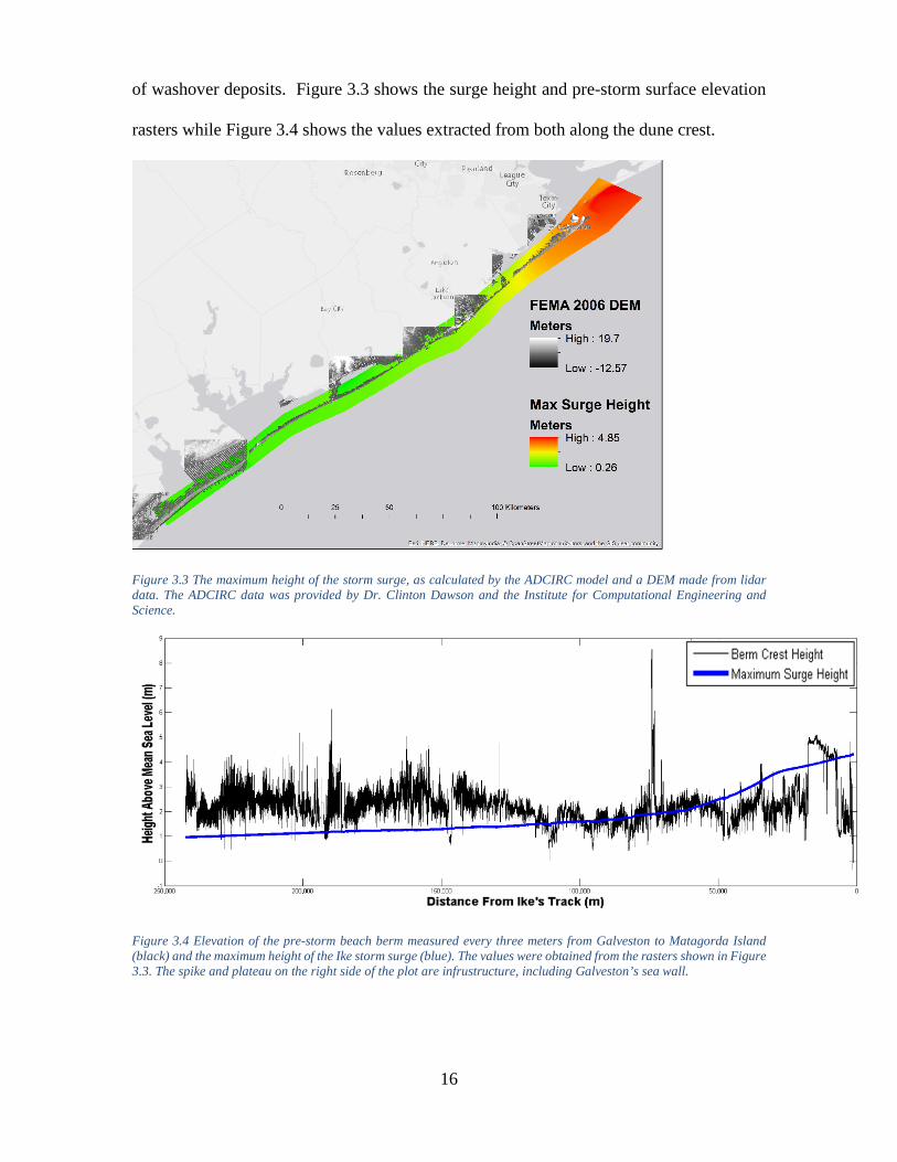
of washover deposits. Figure 3.3 shows the surge height and pre-storm surface elevation
rasters while Figure 3.4 shows the values extracted from both along the dune crest.
Figure 3.3 The maximum height of the storm surge, as calculated by the ADCIRC model and a DEM made from lidar data. The ADCIRC data was provided by Dr. Clinton Dawson and the Institute for Computational Engineering and Science.
Figure 3.4 Elevation of the pre-storm beach berm measured every three meters from Galveston to Matagorda Island (black) and the maximum height of the Ike storm surge (blue). The values were obtained from the rasters shown in Figure 3.3. The spike and plateau on the right side of the plot are infrustructure, including Galveston’s sea wall.

17
Figure 3.5 The locations of the washover deposits shown in Figure. 3.2 are superimposed on the plots of surge and pre-storm berm height from Fig. 3.4. The terms depositional and erosional used here refer only to mapped features, not the coast as a whole. “No Accumulation” is distinct from “Erosional Regime” in that “No Accumulation” indicates the lack of identifiable or measureable deposits, whereas “Erosional Regime” indicates that mapped features can, but do not necessarily show a net loss of sand (Fig 3.9). “Spatially Continuous” means that deposits are either sheetwash, which is laterally extensive, or the fans and terraces are spaced closely together.

18
Figure 3.5 allows for easy comparison of the surge/berm relationship with the gross
locations of washover features. Figure 3.6 shows the ratio of the height of the storm surge
to the height of the pre-storm beach berm, r, calculated at three meters spacing along the
berm.
Figure 3.6.r values represent the maximum height of the storm surge divided by the height of the pre-storm beach crest at locations every three meters along the beach berm. The values generally reflect a gradual decline in the surge height except in places with some local variabiility in berm height.

19
Volumetrics
Figure 3.3.7 The difference map with digitized washover deposits overlain on an aerial photo. The difference map was created by subtracting 2009 Army Corps of Engineers lidar survey data from a 2006 FEMA lidar survey data. Statistics were calculated using each polygon as a zone.
The sum of all elevation difference values provided by the Zonal Statistics tool represents
the net sand change for each mapped washover feature (Fig 3.8, 3.9). The data show that the
washover features are more likely to be net erosional within 60km of where Ike made landfall (Fig
3.9). 60km represents the first point where the surge height becomes equal to the pre-storm berm
height (r=1).

20
Figure 3.8. Volume change for each mapped overwash feature using a lidar difference map and polygons as zones (Fig 3.7). These volumes represent the net addition or removal of sediment from the mapped washover feature. The inset rectangle centered on a zero value for Net Sand Change defines the data range presented in Figure 3.9.
Figure 3.9. Volume change for mapped overwash features using the lidar difference map and polygons as zones. Data shown here are from within the inset shown in Figure 3.8. Data points below the solid horizontal line are net erosional overwash features. Data points above the line are net deposition washover features.

21
Figure 3.10. Mean change in surface elevation associated with each washover feature. This mean change was calculated by taking net-sand change (Fig 3.8) and dividing by surface area of each polygon. Normalizing the data in this way allows us to directly compare all classes of washover deposits.
Figure 3.11 Mean deposit thickness (Fig 3.10) plotted as a function of r (Fig. 3.6). The r value for each feature represents the average for all values measured along the beach berm at the throat position using pre-storm lidar data.
Figure 3.11 shows the mean thickness associated with each mapped feature as a
function of r. In general, deposits with negative thicknesses, the one dimensional indicator
of erosion, require an r value of 0.8 or greater. There was a large concentration of deposits
around an r value of 0.5 and a very few coastline locations with r <0.4. This could lead one
to believe that deposits do not occur unless the r value is around 0.4 or greater, but the
values in Fig. 3.11 are average values, and Figure 3.12 shows that r values were rarely as

22
low as 0.3. This should be considered a boundary condition set by the topography of the
beach and not interpreted as a necessary condition for overwash.
Figure 3.12 All r values less than one plotted as a function of distance from the storm’s landfall in semi-log space. Ike’s storm surge and the Texas coast’s topography only reached a ratio as low as 0.3 in a few locations. This needs to be considered when interpreting figure 3.11.
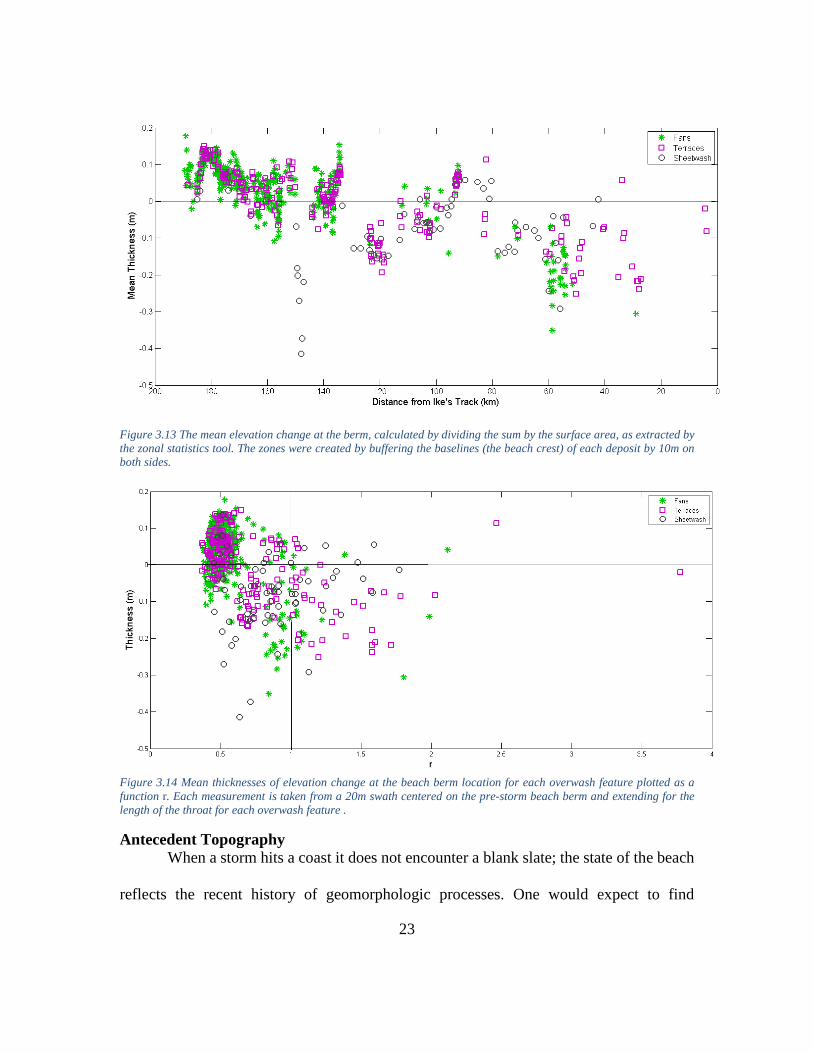
Figure 3.13 shows the mean elevation change (volume/area) isolated at the throat
of each mapped washover feature. The positive values were surprising because I expected
the overwash process to have eroded the berm at these locations. Close inspection of the
post-storm lidar DEM indeed shows sand accumulation in front of and on top of the beach
berm (Fig. 3.15). Figure 3.14 shows the elevation change at the throat plotted against r,
and shows most of the locations that gained mass were associated with smaller r values.
23
Figure 3.13 The mean elevation change at the berm, calculated by dividing the sum by the surface area, as extracted by the zonal statistics tool. The zones were created by buffering the baselines (the beach crest) of each deposit by 10m on both sides.
Figure 3.14 Mean thicknesses of elevation change at the beach berm location for each overwash feature plotted as a function r. Each measurement is taken from a 20m swath centered on the pre-storm beach berm and extending for the length of the throat for each overwash feature .
Antecedent Topography When a storm hits a coast it does not encounter a blank slate; the state of the beach
reflects the recent history of geomorphologic processes. One would expect to find

24
washover deposits preferentially located behind portions of the berm that had been
lowered, removed, or simply present as low topography. However, as shown in Figure 3.5,
there was a segment of coast that was fully inundated regardless of local pre-storm berm
height. This leads to the hypothesis that dependence on low topography should be
negatively correlated with storm energy. Figure 3.16 shows the minimum and mean pre-
storm berm heights for washover fans plotted with distance from the storm. Terraces and
sheetwash were excluded because they are not discrete deposits and cannot be associated
with a specific berm breach location.
Figure 3.15 A stretch of beach in Matagorda County before (above) and after Hurricane Ike, VEx5. The berm is taller after the hurricane, with pronounced gaps where deposits were formed (green polygons). The crest of the berm in the 2006 image is white in places because of missing data, probably because of vegetation.

25
Figure 3.16 Minimum and mean pre-storm berm heights were obtained by creating points along the digitized baselines (the beach crest) of each washover fan and extracting height values. Minima and means were calculated for each deposit using Matlab. The vertical line represents the most distal location where r = 1.
Using the pre-storm DEM I extracted along-berm profiles in locations that I
expected could show a controlling influence of high topography. Figures 3.18-3.20 show
the profiles with locations of washover deposits indicated above, while Figure 3.17 shows
where they come from. These profiles are representative of their areas.

26
Figure 3.17 The locations of the following topographic profiles.

27
Figure 3.18. The topographic profile of the beach berm on Matagorda Island, extracted from the 2006 FEMA DEM. Locations of deposits are plotted at y=5.
Figure 3.19 Topographic profile, with deposits, for an area north of the Colorado river. Figure 3.20 Topographic profile for part of Matagorda Peninsula. Locations of Locations of deposits are plotted at y = 4 deposits are plotted at y = 4
28
CHAPTER 4 Transitions
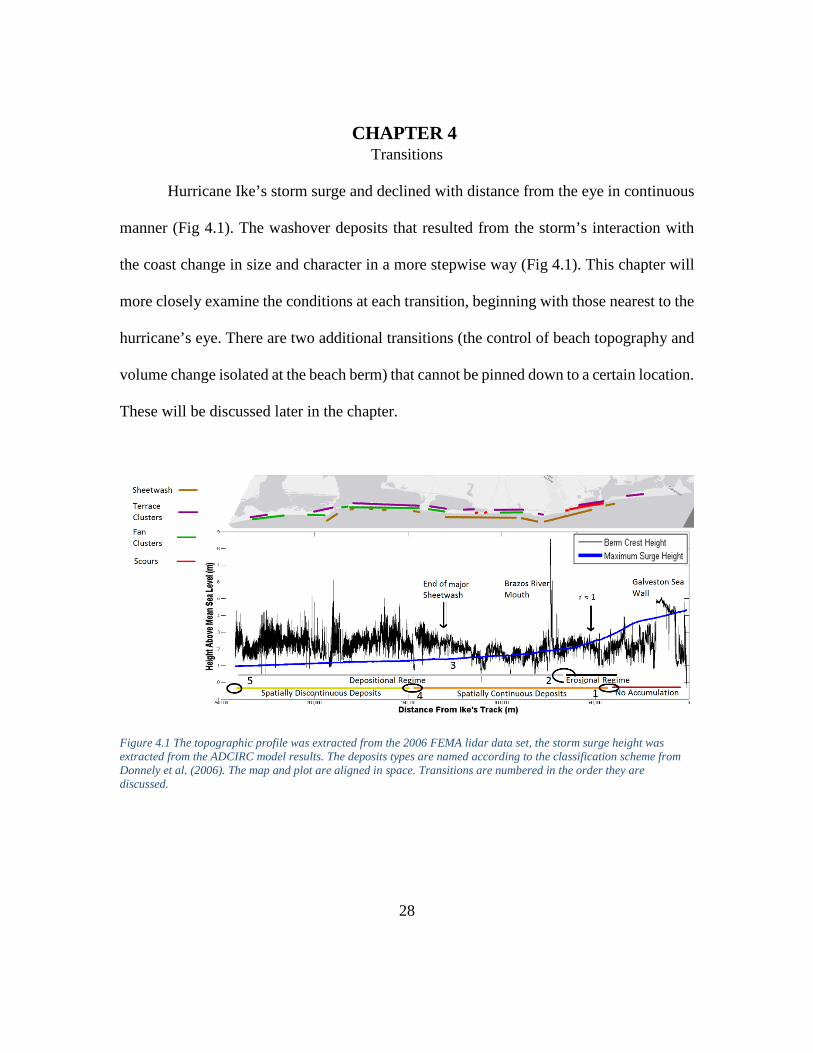
Hurricane Ike’s storm surge and declined with distance from the eye in continuous
manner (Fig 4.1). The washover deposits that resulted from the storm’s interaction with
the coast change in size and character in a more stepwise way (Fig 4.1). This chapter will
more closely examine the conditions at each transition, beginning with those nearest to the
hurricane’s eye. There are two additional transitions (the control of beach topography and
volume change isolated at the beach berm) that cannot be pinned down to a certain location.
These will be discussed later in the chapter.
Figure 4.1 The topographic profile was extracted from the 2006 FEMA lidar data set, the storm surge height was extracted from the ADCIRC model results. The deposits types are named according to the classification scheme from Donnely et al. (2006). The map and plot are aligned in space. Transitions are numbered in the order they are discussed.

29
Figure 4.2 Locations of important transitions. Numbers match those in Figure 4.1.
Transition 1: First Measureable Accumulation
On Galveston Island, close to where the eye of the storm made landfall and where
the storm surge and waves were highest, there were almost no measureable washover
deposits. The few exceptions seem to have accumulated in the presence of infrastructure.
The sediment-transporting conditions exerted by the four meter storm surge and
superimposed waves inhibited deposition of measureable thicknesses within a three
hundred meters of the shoreline by spreading the sediment over a significantly wider area.
The closest location the hurricane’s eye where washover was deposited without noticeable
control by infrastructure is at the southwestern end of Galveston Island (Figure 4.3).
30
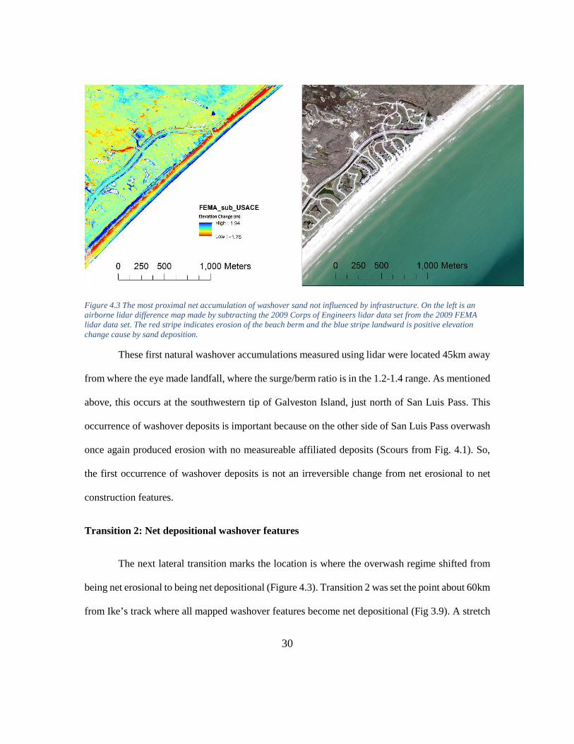
Figure 4.3 The most proximal net accumulation of washover sand not influenced by infrastructure. On the left is an airborne lidar difference map made by subtracting the 2009 Corps of Engineers lidar data set from the 2009 FEMA lidar data set. The red stripe indicates erosion of the beach berm and the blue stripe landward is positive elevation change cause by sand deposition.
These first natural washover accumulations measured using lidar were located 45km away
from where the eye made landfall, where the surge/berm ratio is in the 1.2-1.4 range. As mentioned
above, this occurs at the southwestern tip of Galveston Island, just north of San Luis Pass. This
occurrence of washover deposits is important because on the other side of San Luis Pass overwash
once again produced erosion with no measureable affiliated deposits (Scours from Fig. 4.1). So,
the first occurrence of washover deposits is not an irreversible change from net erosional to net
construction features.
Transition 2: Net depositional washover features
The next lateral transition marks the location is where the overwash regime shifted from
being net erosional to being net depositional (Figure 4.3). Transition 2 was set the point about 60km
from Ike’s track where all mapped washover features become net depositional (Fig 3.9). A stretch

31
of fairly continuous washover deposits occurs over a spatial zone characterized by an r value of
0.85 to 1.2 .
Figure 4.4 Difference map and aerial photo capturing Transition 2. Overwash features to the northeast are predominantly erosional. Mothing to the southwest the swath of erosion systematically decreases while the sedimentation increases until all overwash features are net depositional. This is shown in the difference map by the thinning of the red stripe to the southwest.
Transition 3: End of significant sheetwash deposits
The next important transition marks the end of extensive sheetwash features.
Sheetwash is interpreted to require complete inundation of the beach berm, so its cessation
marks the point where surge height is sufficiently small that local berm topography exerts
control on where washover features are located. For Ike this happened just north of the
mouth of the Colorado River, 150km away from hurricane landfall at an r value of 0.6.
Figure 4.1 shows small amounts of sheetwash southwest of this location, but these are at
the exposed ends of barrier islands and need to be considered separately.

32
Transition 4: Laterally discontinuous washover deposits
The mouth of the Colorado River, which is about 150km from Ike’s track, marks a
transition from nearly continuous washover deposits to spatially separated washover
deposits.. Figure 4.5 shows not only the end of sheetwash but also the end of closely spaced
terrace and fan deposits. Southwest of the Colorado River, deposits formed with more
space in between them. While this transition seems abrupt and centered around the
Colorado River, smaller scale reversals demonstrate that this transition is defined by a zone
of narrow width rather than a point.
Figure 4.5 The location of Transition 4, the mouth of the Colorado River. Deposits have more space in between them to the southwest of the river.

33
Transition 5: Last washover
The last transition among depositional regimes identified here is marked by the last
mapped washover deposit. Beyond this point, it appears that the beach berm was not
breached or overtopped by sediment charged water that could produce washover fans. The
most distal fans I found were about 240km southwest of hurricane landfall at an r value
around 0.35 to 0.45. This location is interesting because it does not possess any obvious
attribute to connect it with the position of the last washover deposits: the surge did not drop
off dramatically and the berm heights varied within a normal range.
Figure 4.6 Aerial photo taken in 2009. The washover deposits farthest from Hurricane Ike's landfall. Arrows are included because the deposits are small.

34
There are two other styles of transitions for which it is harder to identify a single
location, and were therefore excluded from Figure 4.1. These are the (1) control of
antecedent topography and (2) the volume change isolated at the throat of the fan.
Transition 6: Control by antecedent topography
The control that the berm exerts on the locations of deposits is multifaceted. Where
r > 1 the details of preexisting topography can be ignored because all of it is overwhelmed
by the storm surge. Additionally we can assume that sheetwash and closely spaced
washover deposits occur that the berm was being overtopped in spite of its topography.
Figures 3.17-3.19 define a growing dependence on berm topography as distance from the
storm increases and r values decrease. My interpretation of this relative topographic control
is shown in Figure 4.7.

35
Figure 4.7 Interpreted zones of control on location of washover deposition exerted by the local topography of the beach berm. The zone of no control is defined as the extent of significant sheetwash deposits. The other zones were determined by comparing low segments of the berm with the locations of deposits (Figs 3.17-3.19)
As mentioned in Chapter 3, storm inlets and reactivated fans certainly represent low
topography because the berm itself has been removed. Figure 4.8 shows several large
deposits that formed in locations where the beach berm was absent due to previous storms.
These are from Matagorda Peninsula, in the area labelled “Moderate Control” in Figure
4.7.

36
Figure 4.8 Storm inlets and reactivated fans on Matagorda Peninsula
Transition 7: Net volume change at the throat Figure 3.12 shows the trend in volumetric change isolated at the throat of each
deposit. It appears to be a gradual transition from net sand loss to net sand gain, with an
approximately constant rate of change. Figure 4.9 shows the distances from Ike’s track at
which throats change from being erosional to depositional.

37
Figure 4.9 A map view of the data presented in Figure 3.12. Statistics were extracted from the lidar difference map using the buffers shown in Figure 2.2 as zones.

38
Chapter 5
Discussion
Surge/Berm Relationship: r
Coasts are continuously adjusting to environmental forcings. Storms perturb the
background rates of shoreline erosion, but when storm conditions pass the beach begins to
repair itself. The beach we see on any given day is somewhere in this cycle. The most
important processes that restore a beach are a ridge and runnel that works its way from the
nearshore into the swash zone and aggrades the beachface and an aeolian ramp that
accumulates where the beach berm has been scarped (Davis and Fitzgerald 2004: 378).
These two processes do not affect washover deposits, so evidence of larger storms’ impact
on the morphology of the beach complex is more lasting. The most important of those
impacts (Figs. 3.8, 3.9) is delivering sand to the backshore area, landward of the beach
berm, because there it is sequestered yet still available for future coastal processes that keep
a beach healthy, particularly in a regime of sea level rise (Fisher et al. 1974). Therefore it
is important to understand where washover happens, why it happens there, and what exerts
control on it as a process. The spatially comprehensive approach reported herein allows us
to quantify some of these controls by correlating spatial variability in washover with the
spatial variability in storm and beach conditions.
A first order control on the overwash process is the relationship of storm surge to
the height of the beach berm, presented here as the ratio r. If r is greater than one then the
surge overtops the berm regardless of other factors, but as the as r decreases along the coast

39
(Figs 3.4, 3.6) it is almost certain that sediment motion and transport by wave action is
required for overwash to produce measureable changes in berm and back-berm topography.
As shown in Chapter 4 (Figs. 4.1, 4.4) sheetwash, which is understood to require complete
inundation of the beach (Donnelly et al. 2006: p. 968), was found to extend 150 km
southwest along the Texas coast to locations r had a value of only 0.60. This provides a
qualitative indication of importance of waves to washover formation. Farther southwest,
as r generally decreases, the transitions in washover deposit size, style, and character trend
in the direction of smaller, farther-spaced and more dependent on antecedent topography
(Table 5.1). While observed trends are correlated with a decreasing r, it is probable that the
values reported in Table 5.1 are specific to Hurricane Ike and would be different for
hurricanes that approached the coast at a different angle (Penland and Suter 1984), had a
different duration (Morton et al. 2003), or affected a coast with different lithology (Bush
1991). Still, r relates two first-order factors in overwash, the height of the surge and height
of the berm (Morton et al. 2003), and should therefore prove to be a useful quantity in
comparing different hurricanes to each other through their washover deposits. Potentially,
differences in the r values for the same transitions associated with different storms could
provide a measure of the relative contribution of waves in reworking of the beach complex.
40
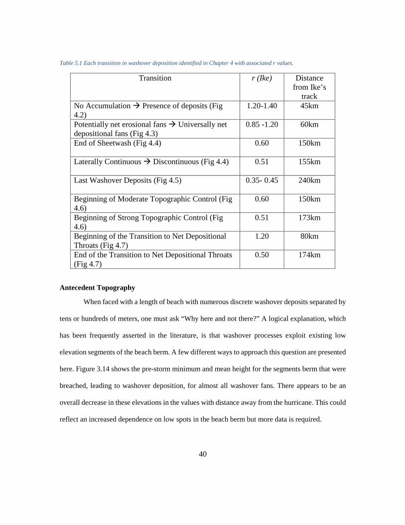
Table 5.1 Each transition in washover deposition identified in Chapter 4 with associated r values.
Transition r (Ike) Distance from Ike’s
track No Accumulation Presence of deposits (Fig 4.2)
1.20-1.40 45km
Potentially net erosional fans Universally net depositional fans (Fig 4.3)
0.85 -1.20 60km
End of Sheetwash (Fig 4.4) 0.60 150km
Laterally Continuous Discontinuous (Fig 4.4) 0.51 155km
Last Washover Deposits (Fig 4.5) 0.35- 0.45 240km
Beginning of Moderate Topographic Control (Fig 4.6)
0.60 150km
Beginning of Strong Topographic Control (Fig 4.6)
0.51 173km
Beginning of the Transition to Net Depositional Throats (Fig 4.7)
1.20 80km
End of the Transition to Net Depositional Throats (Fig 4.7)
0.50 174km
Antecedent Topography
When faced with a length of beach with numerous discrete washover deposits separated by
tens or hundreds of meters, one must ask “Why here and not there?” A logical explanation, which
has been frequently asserted in the literature, is that washover processes exploit existing low
elevation segments of the beach berm. A few different ways to approach this question are presented
here. Figure 3.14 shows the pre-storm minimum and mean height for the segments berm that were
breached, leading to washover deposition, for almost all washover fans. There appears to be an
overall decrease in these elevations in the values with distance away from the hurricane. This could
reflect an increased dependence on low spots in the beach berm but more data is required.

41
Figure 3.16 shows the height of the beach crest on Matagorda Island, which is the most
distal 50km of beach with washover deposits from Hurricane Ike. This area was chosen because it
is where the storm was weakest so control exerted by the berm should be the most obvious. Here
there appears to be a moderately strong correlation between stretches of beach with a low berm and
the presence of washover deposits. The imperfection of this correlation is difficult to understand,
but that is precisely why it holds potential for explaining exactly how overwash happens.
Figure 3.18 shows the berm profile of a kilometer of beach north of the Colorado River
mouth. This segment of coastline appears to be the closest to Hurricane Ike’s track where the
topography of the beach berm can be seen to have exerted some control on the distribution of
washover deposits. The average r value at this location is 0.50. Only 3 km northeast there are linked
washover terraces and fans that were not in any measureable wayaffected by the berm they
overtopped, and the average r value there is 0.60. Figure 3.17 shows the relationship between the
beach berm and the locations of deposits on Matagorda Peninsula. In this case it again seems like
each deposits is located at a local low area in the berm, and the average r value there is 0.44.
Additional evidence for the influence of the beach berm on the positioning of washover
deposits comes from a location on Matagorda Island, at the very distal part of the study area. Figure
18 shows the DEM of a stretch of beach along which the berm has been scarped by a previous
storm and not yet healed. This stretch of beach is also the most distal location where washover
deposits are located within meters to tens of meters from each other. The average r value along this
part of the beach is 0.58.

42
Figure 5.2 Left: 2006 DEM. The beach berm appears to be scarped. Right :The same location after the storm.. This is the most distal group of closely spaced deposits.
Reactivated Fans and Storm Inlets
The largest washover fans by surface area are places where the throats of the fans have
remained open for some time. The gaps in the berm are large and the low topography acts to funnel
water into the throat. Eolian processes that would rebuild the berm across these throats must be
overwhelmed by input from even small storms as well as a perpetually moist surface that inhibits
wind-blown sand transport; the low topography creates positive feedback and the throats are
maintained. Twenty three of the largest twenty five washover fans appear to have been reactivated
by Hurricane Ike. Some of these might properly be considered storm inlets because they connect
to the back barrier lagoon, but others do not. The pull that inlets exert on overwash can be seen in
the concentration of washover features deposited near them and the plan view shapes even appear
to be reaching for the closest access to the lagoon (Fig. 4.8). This bears on the above question of
43
antecedent topography in a slightly different way because it relies on explicit destruction of the
beach berm, not natural variability in its topography.
The highest concentration of storm inlets and reactivated fans, including those in Figure
4.8, was on Matagorda Peninsula north of the Colorado River mouth. While this is speculative, I
believe it is possible that storm inlets routed water into East Matagorda Bay and that this could
have been a contributing factor in causing Transition 4 to occur in this vicinity.
Integrating Waves
Using maps published by Hope et al. (2013), the results of the SWAN wave model run by
Dr. Clinton Dawson, I distributed values for maximum wave height to all points along the storm
modified coast. Integrating these data into my analysis is not straightforward because of the
uncertainty in exactly what is occurring on the beach during a hurricane. Still, waves are a crucial
part of understanding geomorphic change at the beach and they are not evenly distributed along the
coast, so spatial variability in washover cannot be fully understood without them. Figure 5.7 shows
profiles of beach elevation, surge height, and the waves as calculated by the SWAN model and
extracted from the 10m isobath at the time of hurricane landfall.

44
Figure 5.2 Topographic profile from the FEMA 2009 lidar survey, maximum storm surge height from ADCIRC model results and significant wave height. Wave data was created by the SWAN model and provided by the Institute for Computational Engineering and Science. The wave data has a slightly different extent than the other data sets.

45
Also, given that the waves are superimposed on the storm surge it stands to reason that their erosive
power is a function of both those factors and of the height of the berm. To combine these parameters
I multiplied the maximum wave height by the quantity r. The position where the scaled wave height
equals the berm height corresponds nearly perfectly with the end of significant sheetwash deposits
(Fig 5.8). While these plots are intriguing there remains a significant amount of additional work to
be done before we can interpret them with confidence. This is a promising and necessary direction
for future research.
Figure 5.3 Topographic profile from FEMA 2009 lidar survey, surge height from ADCIRC model results and wave data scaled by r. Wave data was extracted from Hope et al. 2013.

46
Understanding Overwash
Because it is rarely feasible to directly observe a beach during a hurricane the details
of the process of overwash are not known with great certainty. We know it requires water
to overtop the beach berm or to erode a throat and flow through it, and we have some
velocity measurements for that flow (2m/s Fisher et al. (1974), 2.4m/s Leatherman (1976)),
but most of these measurements were done on just a few locations on Assateague Island,
so they are not representative larger storms that probably would have destroyed the
equipment used to take measurements. Donnelly et al. 2006 report that the following four
step model provided by Fisher et al. 1974 is basically correct but the order of the steps can
be reversed or repeated.
1. Erosion in the throat
2. Deposition of sand on the fan and in the bay
3. As storm intensity decreases, overwash bore velocities decrease and sand is
deposited on the throat and in the fan
4. The washover is reworked by abating storm winds.
While this model might be accurate, the finding that the area of the beach berm,
through which the throats are eroded, transitions from being net erosional to net
depositional with a fairly constant rate of change (Fig 3.11) demands additional attention.
If the berm experienced net accretion in places with washover deposits can we be sure it
was breached? This question could probably be answered by finding an erosional surface
with ground penetrating radar, but local governments discourage activity that might

47
damage the vegetation on the berm. The results presented here have been mostly in
reference to identified and digitized washover deposits, but the state of the beach as a whole
clarifies the erosion/accretion trend because the entire beach is behaving in the same way.
Notwithstanding deposits, the beach berm becomes net depositional gradually with
distance from Ike’s track, so the transition from net negative to net positive washover
throats simply fits into this larger trend. It is possible that the stages listed above occurred
in that order but the deposition step shows a spatial trend that obscures the history of
erosion for distal washover deposits.
Washover sand is transported as the flow spreads and decelerates and we have
indications that this can occur before the hurricane even makes landfall (Shaw et al. 2010).
The deposits retain the morphology that reflects this landward transport activity, and this
does not seem to change with distance along the coast. This means that even during a storm
they are not reworked while they are subaqueous. This seems to indicate that storms have
a coupled destructive/constructive or erosional/depositional phase, past which the water
that inundates the beach acts to protect washover deposits. There was no clear signal that
abating storm winds affected washover deposits during Hurricane Ike, but observations at
the beach certainly indicate significant aeolian reworking since the storm. Sand that Ike
pushed onto the beach is now circulating in dune fields that serve as habitats and act to
dissipate energy that could otherwise exert itself on infrastructure or people.

48
Chapter 6
Conclusions
The alongshore distribution of washover deposits caused by a hurricane is
controlled by the strength and duration of the storm and the geometry of the beach. The
most important input from the storm is the surge because it can simply destroy the berm
and drown the beach. Where the surge is greatest measureable volumes of sand are not
deposited behind the berm crest at all because the very large transport distances appear to
produce a resulting deposit that is very thin. Moving along shore and down the decreasing
storm energy gradient, this washover state gives way to sheetwash and other laterally
continuous deposits, then to clusters of washover fans and terraces that are increasingly
spaced farther apart, and eventually there is a point where the storm waters could not
overtop the beach berm. These transitions are more stepwise than the gradual decrease in
the surge height and are not unidirectional at small spatial scales (Fig 3.5). There are clear
indications waves play a crucial role in damaging or lowering the beach berm during a
storm but it is hard to quantify.
Within 60km of Hurricane Ike’s track it was possible for the area mapped as a
washover feature to have experienced a net loss of sand but beyond that point almost all
mapped features experienced net aggradation. While sheetwash and terraces naturally
contain more sand, after normalizing the volume change by the areal extent of each deposit
it appears there is no significant difference between the three classes of washover presented
here. The volume change isolated at the throats showed a gradual transition from net
erosion to net deposition, which mirrors the pattern in volume change on the shoreface.
Ike’s surge and waves were completely effective at destroying or topping the beach
berm up to the point that the surge was 60% as high as the pre-storm berm. At that point

49
deposits preferentially formed where the berm was lower or previously damaged. Where r
was 0.50 or lower, the berm exerted a much stronger control on where washover deposits
formed.
The identified inconsistencies in between the erosion/deposition ascribed to the
surge and the state of the beach when Hurricane Ike passed are assumed to be the product
of wave action. This is a promising avenue for future research. The deposition of a body
of sheetwash on Matagorda Peninsula was shown to have occurred the day before landfall,
during the period of maximum wave heights, though the amount of work required to make
that determination is prohibitive for expanding the methods to numerous other washover
deposits (Shaw et al. 2015). With the timing of deposition known, we can begin to move
towards a fuller understanding of the overwash process that might yield a deterministic
relationship between surge, waves, and the beach.
By improving our understanding of what controls overwash processes, we can
improve our long term predictions of coastal change. Sea level rise and the huge
populations in coastal areas makes this an issue of paramount importance for economic and
security reasons.

50
Bibliography Berg, Robbie. 2009. Tropical Cyclone Report: Hurricane Ike. National Hurricane Center Bush, D.M., 1991. Impact of Hurricane Hugo on the rocky coast of Puerto Rico. Journal
of Coastal Research, SI #8, 49-67. Fort Lauderdale (Florida). ISSN 0749-0208 Davis, Richard A. and Duncan M. Fitzgerald. 2004. Beaches and Coasts. Blackwell Publishing, Malden MA Donnelly, Chantal, Nicholas Kraus, and Magnus Larson. 2006. State of Knowledge on
Measurement and modelling of Coastal Overwash. Journal of Coastal Research. 22:4. 965-991
East, Jeffery W., Michael J. Turco, and Robert R. Mason Jr. 2008. Monitoring Inland
Storm Surge and Flooding from Hurricane Ike in Texas and Louisiana, September 2008. USGS open file report 2008-1365
Hope, M. E., et al. (2013), Hindcast and validation of Hurricane Ike (2008) waves,
forerunner, and storm surge, J. Geophys. Res. Oceans, 118, doi:10.1002/jgrc.20314.
IPCC Climate Change 2013: The Physical Science Basis (eds Stocker, T. F. et al)
Cambridge University Press Kennedy, Andrew B., Uriah Gravois, Brian C. Zachary, Joannes J. Westerink, Mark E.
Hope, J. Casey Dietrich, Mark D. Powell, Andrew T. Cox, Richard A. Luettich Jr. and Robert G. Dean. 2011. Origin of the Hurricane Ike forerunner surge. Geophysical Research Letters 38: L08608
Lambeck et al. 2004. Sea level and global ice volumes from the Last Glacial Maximum
to the Holocene. Proceedings of the National Academy of Sciences. 111:43, 15296-152903
Larson, Erik. 2000. Isaac’s Storm: A Man, a Time, and the Deadliest Hurricane in
History. Random House. McGowen, J.H., Garner, L.E. and Wilkinson, B.H., 1977. The Gulf shoreline of Texas:
processes, characteristics, and factors in use. Bureau of Economic Geology. Morton, R.A.; Guy, K.K.; Hill, H.W., and Pascoe, T., 2003. Regional Morphological
Responses to the March 1962 Ash Wednesday Storm. In: Proceedings Coastal

51
Sediments ’03. Corpus Christi,Texas: World Scientific Press and East Meets West Productions, CD-ROM, 11p.
Morton, R.A. and Sallenger, A.H., Jr., 2003. Morphological impacts of extreme storms
on sandy barriers. Journal of Coastal Research, 19(3), 560-573. Penland, S. and Suter, J.R., 1984. Low-profile barrier island overwash and breaching in
the Gulf of Mexico. In: Proceedings 19th Coastal Engineering Conference (Houston, Texas, ASCE), pp.2339–2345.
Rogers, L.J., L.J. Moore, E.B. Goldstein, C.J. Hein, J. Lorenzo-Trueba, and A.D.
Ashton. 2015. Anthropogenic Controls on Overwash Deposition; Evidence and Consequences. J. Geophys. Res. Earth Surf., 120, 2609-2624
Shaw, John, Yao You, David Mohrig, and Gary Kocurek. 2015. Tracking hurricane-generated storm surge with washover fan stratigraphy. Geology 43 (2): 127-130
Stutz, Matthew L. and Orrin H. Pilkey. 2011. Open-Ocean Barrier Islands: Global
Influence of Climatic, Oceanographic, and Depositional Settings. Journal of Coastal Research 27:2, 207 – 222
Texas Strategic Mapping Program (StratMap). 2009. TOP – 2008/2009 0.5 Meter DOQQ
Metadata. 2009-2009. 2008-2009 Texas Orthoimagery Program. Austin TX Young, Robert S. “The Beach Boondoggle” The New York Times [New York City] 12
Oct. 2016. A23


