DESIGN OF WATER SUPPLY SCHEME FOR EWS HOUSES IN AGRA,
UTTAR PRADESH, INDIA 1Dr. Sohail Ayub and
2Aditya Kumar Agarwal
1Associate Professor, Civil Engineering Department 2Research Scholar, Environmental Engineering Department
Aligarh Muslim University (AMU), Aligarh
Abstract: The research paper highlights the recent work carried out on the water quality status and water supply near Kalindi Vihar Colony, Tedi Bagiya, Agra, India. The Current research has been carried out on Ground water quality in the area in order to design a water supply scheme for an under developing residential colony i.e. EWS houses there. It also includes the provision of design of water treatment scheme for the area in order to supply the treated water to the houses. Keywords: Water, Surface Water, Ground Water, Water Quality, Water Supply, Water Treatment Scheme.
1. Introduction
The research site is located in the district of Agra in the state of Uttar Pradesh, India. The site
is located near Kalindi Vihar, Tedi Bagiya on the outskirts of the city of Agra.
1.1 Agra formerly known as Akbarabad is a city on the banks of the river Yamuna in the
northern state of Uttar Pradesh, India, 363 kilometer west of state capital, Lucknow and 200
kilometers south from national capital New Delhi. The modern city of Agra was founded way
back in the 16th century by Sikandar Lodhi, who was a king of the Lodhi dynasty. In
geographical terms, the city of Agra lies between 26°44’ N to 27°25’N and 77°26’E to
78°32’E. The city is located at an average altitude of 171 meters or 561 feet above the sea
level. Agra features a semiarid climate that borders on a humid subtropical climate. The city
features mild winters, hot and dry summers and a monsoon season. It is one of the most
populous cities in Uttar Pradesh and the 19th most populous in India. Agra district population
grew by 21% in the decade 2001-2011 and 31% in the decade 1991–2001. On the basis of
landmass, Agra is the third largest city in the state of Uttar Pradesh. Because 80 % of the
city's sewage flows into Yamuna River, it is 20th most polluted city in India. Agra Airport
(Kheria Airport) is about 12.5 km from city center. Agra is on the central train line
between Delhi and Mumbai (Bombay) and between Delhi and Chennai. Agra is famous for
its Historical monuments like Taj Mahal, Agra Fort, Sikandra, Fatehpur sikri, etc.
International Journal of Science, Environment and Technology, Vol. 2, No 2, 2013, 211 - 229
�
Received Feb 25, 2013 * Published April 2, 2013 * www.ijset.net
212 Dr. Sohail Ayub and Aditya Kumar Agarwal
1.2 Research Site: As mentioned above the site is located on the outskirts of the city. The
geographical location of the work site is about 27°22’N, 78°08’E. The Site is located near
NH 2 (towards Tundla) which connects Agra to Kanpur. From Aligarh it is about 80 km and
it takes about 2 hrs to reach the site travelling on NH 93 which connects Agra to Aligarh. At
proposed work site, EWS (Economically Weaker Section) Houses are to be constructed for
economically backward section of society. This Project comes under the proposed Welfare
Scheme of “Manyawar Shri Kanshiram Ji Shahri Garib Awas Yojna” undertaken by the
erstwhile Government of Uttar Pradesh led By Shrimati Mayawati Ji. The work is being
handled by U.P. Housing & Development Board under the supervision of Agra Development
Authority. The site is an extension of Kalindi Vihar Yojana of Agra Development Authority,
under Sector – H. Under the proposed work, 337 houses are to be built.
1.3 Objective of Study: The main objective of the study was to propose a water supply
scheme for the above mentioned project of 337 houses. Other works included finding out
possible location of sources of water in the area, testing of the water quality, comparison of
those values with standards specified by the government. Proposal of water treatment
technologies depending upon the results of water quality tests carried out in the whole area.
Water quantity estimation, population estimation, design of intake structures, and pumping
apparatus, mode of conveyance of water, Water Storage structures and finally water supply
network (water distribution network).
2. Water Quality Parameters:
Public, in general, judges the quality of water supplied based on its appearance, taste and
odor at the point of its use. Although appearance, taste, odor etc., are useful indicators of the
quality of drinking water, their presence may not necessarily make water unsafe to drink. In
the same way, the absence of any unpleasant qualities does not guarantee water to be safe for
consumption. True that drinking water should be aesthetically pleasing, ideally looking clear,
colorless and well aerated with no unpalatable taste and odor. However, suitability in terms of
public health is determined by microbiological, physical, chemical and radiological
characteristics. Of these, the most important is microbiological quality. Also a number of
chemical contaminants (both organic and inorganic) are found in water. These cause health
problems in the long run and, therefore, detailed analyses are warranted. The drinking water,
thus, should be:
• Free from pathogenic (disease causing) organisms.
• Clear (with low turbidity and little color).
�����������������������������������������������������Design of Water Supply Scheme for …………. 213
• Not saline (salty in taste).
• Free from offensive taste or smell.
• Free from compounds that may have adverse effects on health or harmful in long
term.
• Free from chemicals that cause corrosion of water supply system or stain clothes
washed using it.
To ensure safe drinking water, detailed quality standards for physical, chemical,
microbiological and radiological characteristics of water have been proposed by different
countries and international organizations.
3. Laboratory Analysis of Water Quality:
Materials & Methods:
After initial survey of the site, following notable features were found out:
a) Source of water: Ground water b) Mode of water: Bore - well
3.1 Sampling: The water samples were brought from the Agra and analyzed for different
parameters in the Environmental engineering laboratory of Civil engineering department,
Z.H.C.E.T, Aligarh Muslim University, Aligarh, Uttar Pradesh, India. Dark plastic bottles of
2 liters capacity each with a stopper were used for collecting samples. Each bottle was
washed with 2% Nitric acid and then rinsed three times with distilled water. The bottles were
then preserved in a clean place. The bottles were filled leaving no air space, and then the
bottle was sealed to prevent any leakage and stored in a cool place. Each container was
clearly marked with the name, location and date of sampling.
3.2 Sampling Points: After initial survey of the site, the study area was divided suitably into
four parts depending upon the location of source of water. Thus a total of four samples were
taken from the whole area from the location of source of water randomly. In the first week of
sampling, samples from two points were taken in two bottles of 2 liters each. Similarly in
next week, samples from the other two points were taken in two bottles of 2 liters each. The
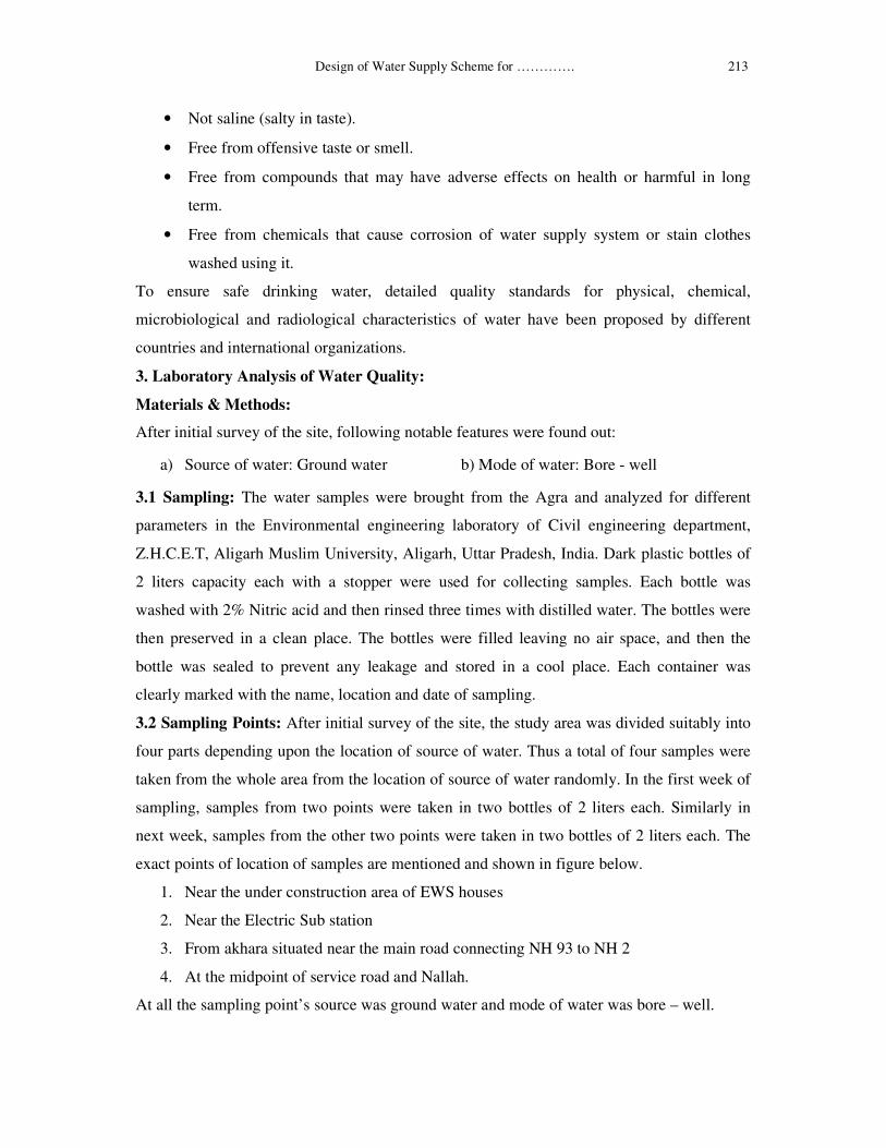
exact points of location of samples are mentioned and shown in figure below.
1. Near the under construction area of EWS houses
2. Near the Electric Sub station
3. From akhara situated near the main road connecting NH 93 to NH 2
4. At the midpoint of service road and Nallah.
At all the sampling point’s source was ground water and mode of water was bore – well.
214 Dr. Sohail Ayub and Aditya Kumar Agarwal
�
Figure 3.1 Aerial Photograph showing the Location of Sampling Points
3.3 Water Quality Parameters tested in the laboratory: Following parameters were tested in
the laboratory:
3.3.1 pH
3.3.2 Turbidity: Nephelometer Method
3.3.3 Temperature
3.3.4 Sulphate: Nephelometer Method
3.3.5 Alkalinity
3.3.6 Total Hardness: EDTA Titration Method
3.3.7 Dissolved Oxygen, DO: Winkler Azide modified Titrimetric Method
3.3.8 Biochemical Oxygen Demand BOD: Winkler Azide modified Titrimetric Method
3.3.9 Chloride: Argentometric Titration Method
3.3.10 Total Solids
3.3.11 Chemical Oxygen Demand COD: Closed Reflux Titrimetric Method
3.3.12 Fluoride: SPANDS Spectrophotometric method using HACH instrument DR 5000
Method no. 8029
3.3.13 Nitrate: Spectrophotometer Method using HACH DR 5000 series, Method 8039,
Cadmium Reduction Method, Powder pillows.
3.3.14 Iron: Spectrophotometer Method using HACH DR 5000 series, Method 8146, 1, 10
Phenanthroline Method, Powder pillows.
�����������������������������������������������������Design of Water Supply Scheme for …………. 215
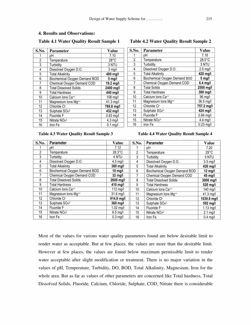
4. Results and Observations:
Table 4.1 Water Quality Result Sample 1 Table 4.2 Water Quality Result Sample 2
S.No. Parameter Value �� ��� �����
�� ��� ���� �������
�� ��������� �����
�� ��������� !�"#��� �� �����"$��
�� �� ��%�& ��#���� ���������
'� (��)*��) �� !�"#��� #��( �� ������
�� �*��) �� !�"#��� #��� �� ��������
�� �� ��+������ ���������
,� �� ��� ��#��� � �������
�-� � �)����.�#��� //� ,'��"$��
��� 0 "#�����.�#��0"//� �'����"$��
��� �*��������1� ����������
��� +���* ��+ ��1� ���������
��� 2�������21� -�����"$��
��� ���� ��� ��1� �����"$��
�'� .��#�2� -�����"$���
Table 4.3 Water Quality Result Sample 3 Table 4.4 Water Quality Result Sample 4
�
Most of the values for various water quality parameters found are below desirable limit to
render water as acceptable. But at few places, the values are more than the desirable limit.
However at few places, the values are found below maximum permissible limit to render
water acceptable after slight modification or treatment. There is no major variation in the
values of pH, Temperature, Turbidity, DO, BOD, Total Alkalinity, Magnesium, Iron for the
whole area. But as far as values of other parameters are concerned like Total hardness, Total
Dissolved Solids, Fluoride, Calcium, Chloride, Sulphate, COD, Nitrate there is considerable
S.No. Parameter Value �� ��� ���-�
�� ��� ���� �����
�� ��������� �����
�� ��������� !�"#��� �� ���"$��
�� �� ��%�& ��#���� ���������
'� (��)*��) �� !�"#��� #��( �� ������
�� �*��) �� !�"#��� #��� �� � ��������
�� �� �����������+������ ����������
,� �� ��� ��#��� ���������
�-� � �)����.�#��� //� �-���"$��
��� 0 "#�����.�#��0"//� ������"$��
��� �*��������1� � ��������
��� +���* ��+ ��1� ���������
��� 2�������21� -�����"$��
��� ���� ��� ��1� �����"$��
�'� .��#�2� -����"$��
S.No. ���������� Value �� ��� �����
�� ��� ���� �������
�� ��������� �����
�� ��������� !�"#��� �� �����"$��
�� �� ��%�& ��#���� ���������
'� (��)*��) �� !�"#��� #��( �� ��������
�� �*��) �� !�"#��� #��� �� ��������
�� �� �����������+������ ���������
,� �� ��� ��#��� ���������
�-� � �)����.�#��� //� �����"$��
��� 0 "#�����.�#��0"//� ���'��"$��
��� �*��������1� ����������
��� +���* ��+ ��1� ��������
��� 2�������21� ��-���"$��
��� ���� ��� ��1� '����"$��
�'� .��#�2� -����"$��
S.No. ���������� Value �� ��� ���-�
�� ��� ���� �,���
�� ��������� �����
�� ��������� !�"#��� �� �����"$��
�� �� ��%�& ��#���� ���������
'� (��)*��) �� !�"#��� #��( �� ��������
�� �*��) �� !�"#��� #��� �� �������
�� �� �����������+������ ����������
,� �� ��� ��#��� ��������
�-� � �)����.�#��� //� ��-��"$��
��� 0 "#�����.�#��0"//� ������"$��
��� �*��������1� ��� ��������
��� +���* ��+ ��1� �������
��� 2�������21� ������"$��
��� ���� ��� ��1� �����"$��
�'� .��#�2� -����"$��
216 Dr. Sohail Ayub and Aditya Kumar Agarwal
variation in the values obtained for the whole area. pH, Temperature, Turbidity of all the
samples were within desirable limits. As far as Values of BOD are concerned, sample’s 1, 2,
3 are within maximum permissible limits. The value of DO for the area is also less. In the
present study area, Phenolphthalein Alkalinity was absent from all the samples which
indicates absence of Hydroxyl and carbonate ions and presence of bicarbonate ions. Value of
Chloride is high, more than desirable limit and for the sample 4 it is more than maximum
permissible limit. Value of Sulphate is very high almost unacceptable for all the samples
collected from the area, barring sample 3 where it is just below the maximum permissible
limit. Water is very hard and needs to be treated. Value of TDS is also very high and is
unacceptable for all the samples and needs to be properly treated. Value of Fluoride, Iron is
within desirable limit for most of the samples. Arsenic is absent from water, which indicates
in general the absence of most of the heavy metals and highly poisonous ions from water. In
general, water in the area is acceptable to a certain limit only and needs to be further treated
before being supplied to houses especially for drinking purposes. The treatment of water
should involve such a scheme that would effectively, efficiently remove / reduce TDS,
hardness, alkalinity, sulphate, and chlorides to render water suitable for public use. The
treatment scheme will be discussed in detail in the next chapter. The high values obtained for
TDS, Alkalinity, Hardness, Chloride and Sulphate can be attributed to the location of
Municipal Solid Waste Landfill (Sharda Landfill) in the vicinity of the site.
5. Population Forecast:
Known: Number of EWS houses: 337
Assumption: People expected to be living in each house (average): 3
Total Expected Population of the EWS houses area (2012): 337 X 3 = 1011
Estimation of future population in the area by geometrical increase method:
From the census records, % increase in population is as: 20.5, 21.2, 20, 31 and 20.1
Geometric mean rg = (0.205 x 0.212 x 0.20 x 0.31 x 0.201) ^ (1/5) = 0.2222
Population of the area in 2020 = Population in 2012 X (1 + rg) 0.8
= 1011 X (1 + 0.2222) 0.8 = 1187
Population of the area in 2042 = Population in 2012 X (1 + rg) 3
= 1011 X (1 + 0.2222) 3 = 1845
6. Water Demand:
Expected Population for 2012: 1011
Expected Population for 2042: 1845
�����������������������������������������������������Design of Water Supply Scheme for …………. 217
Average rate of water supply as per Indian standards = 135 lpcd
(Including domestic, commercial, public, and wastes)
Water required for whole area for population expected as of 2012 = 1011 x 135 = 136485
l/day = 0.14 MLD
Water required for whole area for population expected as of 2042 = 1845 x 135 = 249075
l/day = 0.25 MLD
Assume, Peak Factor = 1.2
Peak daily demand for 2012 population = 0.14 x 1.2 = 0.17 MLD
Peak daily demand for 2042 population = 0.25 x 1.2 = 0.3 MLD
The whole system is to be designed for the future population of 2042 that is design
period of 30 years assumed at the beginning only.
6.1 Design Capacity for Various Components
(i) Intake structure daily demand = 0.3 MLD
(ii) Pipe main = 0.3 MLD
(iii) For units at the treatment plant = 0.3 MLD
(iv) Lift Pump = 1.5 x 0.3 = 0.45 MLD
7. Intake Structures:
1. Intake Well
1 a. Design Flow Rate – 0.3 MLD
1 b. Design
i) Number – 1
ii) Velocity of flow – 0.75 m/second
iii) Detention time – 10 minute
iv) Depth – 4 m
v) Diameter – 0.82 m
2. Pen Stock
i) Number of pen stock for each intake well - 2
ii) Velocity through pen stock - 0.6 m/sec
iii) Depth – 3 m
iv) Diameter – 0.06 m
3. Bell Mouth Strainer
i) Velocity of flow - 0.25 m/sec
ii) Diameter – 0.13 m
218 Dr. Sohail Ayub and Aditya Kumar Agarwal
4. Gravity Main
i) Velocity – 0.7 m/sec
ii) Diameter – 0.08 m
5. Jack Well
i) Detention Time – 5 min
ii) Diameter – 0.67 m
iii) Suction Depth – 7 m
iv) Overall Depth – 9 m
6. Rising Main
(i) Velocity – 1 m/sec
(ii) 0.07 m
7. Pump
i) Design Flow Rate – 0.45 MLD
ii) Pump Efficiency – 75 %
iii) Number – 2 in parallel of which 1 is as standby
iv) Power – 1 HP (0.75 kW)
8. Water Treatment Technologies:
As per the results obtained from water quality analysis, it can be seen that the water in the
area is having high amount of TDS, Hardness, Alkalinity, Chloride, Sulphate which renders
the water unsuitable for drinking and various other purposes. So it needs to be treated.
TDS, Hardness, Chloride, Sulphate can be removed by Reverse Osmosis. Hardness and
Alkalinity can also be reduced by Chemical Precipitation: Water softening (Lime Soda
Softening). Both the above mentioned process is dealt in detail below.
8.1 Chemical Precipitation: Lime- Soda Ash Water Softening
8.1.1 Calculation of Lime – Soda Ash Dosage
For calculation of quantity of lime and soda required for treating the water in the area, values
of water quality test result of sample 4 is taken as they are the maximum for the whole area.
The idea behind this is to treat the maximum value and subsequently the lesser values will be
treated automatically.
Sample 4
The water parameters used to calculate the dosages are:
Water flow rate = 0.30 MLD = 300 m3/day
pH = 7.2
�����������������������������������������������������Design of Water Supply Scheme for …………. 219
Total Alkalinity = 420 mg/l
Total Hardness = 520 mg/l
Calcium, Ca2+ = 140 mg/l
Magnesium, Mg2+ = 41.3 mg/l
Chloride, Cl- = 1039.7 mg/l
Sulphate, SO42- = 592 mg/l
As Total Alkalinity < Total hardness, Carbonate Hardness = Total Alkalinity = 420 mg/l
Non Carbonate Hardness = Total Hardness – Carbonate hardness = 520 – 420 = 100 mg/l
As pH = 7.2, So Total Alkalinity will be due to HCO3- only.
Hence, HCO3- = 420 mg/l = 420 / 61 = 6.88 meq/l
Ca2+ = 140 mg/l = 140 / 20 = 7 meq/l
Mg2+ = 41.3 mg/l = 41.3 / 12 = 3.45 meq/l
SO42- = 592 mg/l = 592 / 48 = 12.33 meq/l
Cl- = 1039.7 mg/l = 1039.7 / 35.5 = 29.29 meq/l
Hardness causing species:
Ca (HCO3)2 = 6.88 meq/l, CaSO4 = 0.12 meq/l, MgSO4 = 3.45 meq/l
Chemical Reactions Involved:
i) Ca(HCO3)2 + Ca(OH)2 = 2 CaCO3 (�) + 2 H2O.
ii) CaSO4
+ Na2CO
3 = CaCO3 (�) + Na
2SO
4
iii) a. MgSO4 + Ca(OH)2 = Mg(OH)2 (�) + CaSO4
b. CaSO4
+ Na2CO
3 = CaCO3 (�) + Na
2SO
4
Lime Required:
Lime required in form of Quick lime CaO (M.W. = 56, Equivalent Weight = 56 / 2 = 28)
Lime required = 6.88 + 3.45 + 1.25 (excess lime to raise pH) = 11.58 meq/l
= 11.58 (meq/l) X 28 X 300 (m3/day)
= 97272 g/day = 97.27 kg/day
Purity of lime provided in the market = 90 %
Total lime required = 97.27/0.9 = 108.10 (kg/day) X 365 (day/year) = 39456 kg/year = 39.46
metric tons/year.
Cost of lime @ present market rate of 90 $ per metric ton
= 39.46 X 90 X 54 = Rs. 1, 91,776 /- per year (INR)
Soda Ash Required:
Soda ash required in form of Na2CO3 (M.W. = 106, Equivalent Weight = 106 / 2 = 53)
220 Dr. Sohail Ayub and Aditya Kumar Agarwal
Soda ash required = 3.45 + 0.12 = 3.57 meq/l
= 3.57 (meq/l) X 53 X 300 (m3/day) = 56763 g/day = 56.76 kg/day
Purity of Soda ash in the market = 90%
Total Soda ash required = 56.76/0.9 = 63.07 (kg/day) X 365 (day/year) = 23020 kg/year =
23.02 metric tons/year
Cost of Soda ash @ present market rate of 225 $ per metric ton
= 23.02 X 225 X 54 = Rs. 2, 79,693 /- per year (INR)
This method reduces the calcium hardness to 40 mg/l as CaCO3 and magnesium hardness to
10 mg/l as CaCO3. Hence finished water will have 50 mg/l of carbonate hardness only.
Recarbonation required: addition of CO2 to maintain pH. Recarbonation is done in single
stage only in settling tank. Amount of CO2 required = 1.25 meq/l (to remove excess lime).
8.1.2 Design of Various Treatment Units
8.1.2.1 Chemical Storage Room: Provide a room of dimension = 10 m X 8.5 m
8.1.2.2 Rapid Mixing Tank:
i) Detention Time – 50 seconds
ii) Velocity Gradient – 600 /seconds
iii) Diameter – 0.57 m
iv) Depth – 1 m
v) Rotational Speed of Impeller – 120 rpm
vi) Diameter of Impeller – 0.24 m
vii) Velocity of tip of Impeller – 1.5 m/sec
viii) Power Required – 63.18 Watts
ix) Blades Number – 5
x) Blades Size – 0.1 m X 0.11 m
8.1.2.3 Sedimentation Tank:
i) Removal efficiency – 80 %
ii) Surface Overflow Rate – 33.5 m/day
iii) Detention Time – 2.5 Hours
iv) Diameter of Tank – 3.38 m
v) Depth of Tank – 3.48 m
vi) 90° V – Notch Number – 53
vii) Spacing Between two Notches – 20 cm
viii) Depth of Notch – 5 cm
�����������������������������������������������������Design of Water Supply Scheme for …………. 221
ix) Effluent Box Size - 1 m X 1m
x) Diameter of Outlet Pipe – 1 m
xi) Effluent Launder Size – 0.4 m Width X 0.33 m Depth
8.1.2.4 Rapid Sand Gravity Filter:
i) Rate of Filtration – 4 m3/m2/hour ii) Number of Filters – 2 , 1 as a standby iii) Diameter of Filter – 1.83 m iv) Depth of Filter – 1.5 m v) Effective Size of Sand for Filter – 0.5 mm
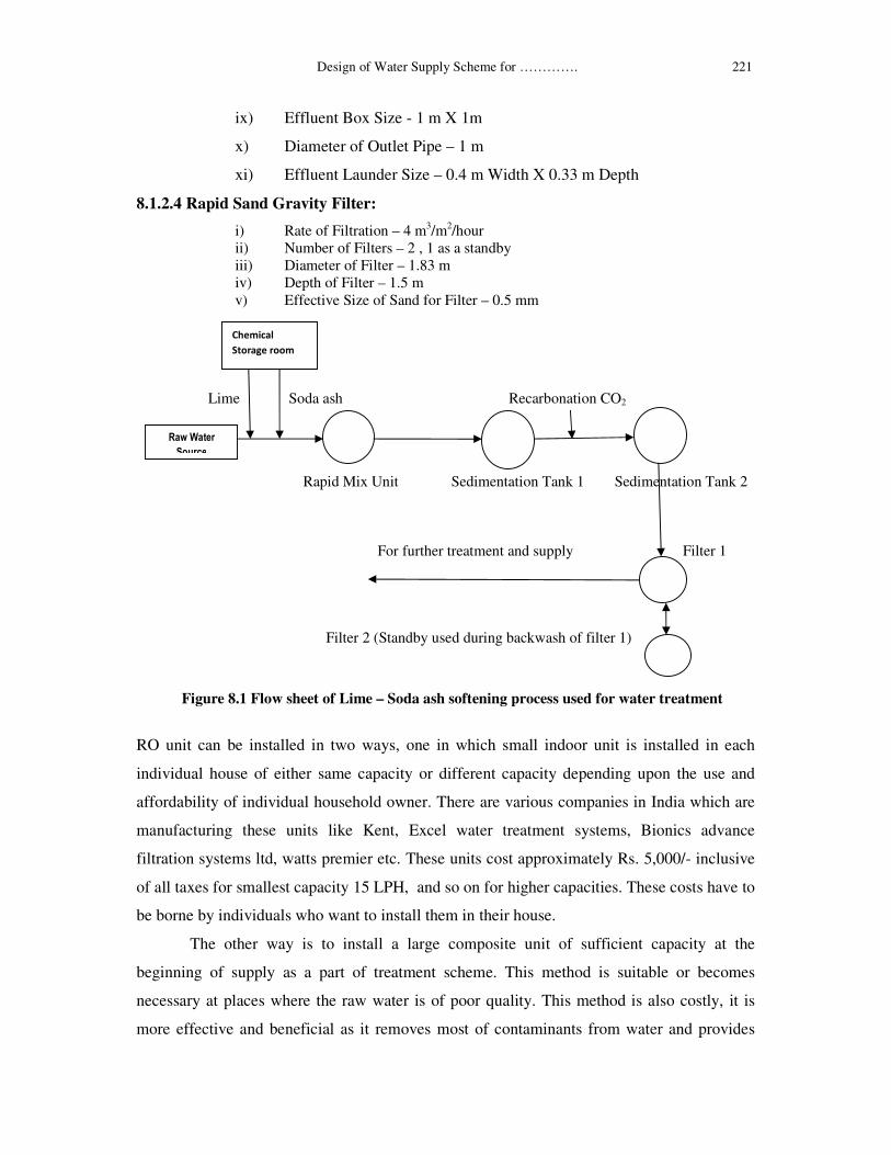
Lime Soda ash Recarbonation CO2
Rapid Mix Unit Sedimentation Tank 1 Sedimentation Tank 2 For further treatment and supply Filter 1 Filter 2 (Standby used during backwash of filter 1)
Figure 8.1 Flow sheet of Lime – Soda ash softening process used for water treatment
RO unit can be installed in two ways, one in which small indoor unit is installed in each
individual house of either same capacity or different capacity depending upon the use and
affordability of individual household owner. There are various companies in India which are
manufacturing these units like Kent, Excel water treatment systems, Bionics advance
filtration systems ltd, watts premier etc. These units cost approximately Rs. 5,000/- inclusive
of all taxes for smallest capacity 15 LPH, and so on for higher capacities. These costs have to
be borne by individuals who want to install them in their house.
The other way is to install a large composite unit of sufficient capacity at the
beginning of supply as a part of treatment scheme. This method is suitable or becomes
necessary at places where the raw water is of poor quality. This method is also costly, it is
more effective and beneficial as it removes most of contaminants from water and provides
����������
�������
��������
�� ��� ���
222 Dr. Sohail Ayub and Aditya Kumar Agarwal
clean and clear water to everyone which can be used for all purposes. There are various
companies in India who are manufacturing these units like Excel water treatment systems
limited, aqua puro systems limited, H2O systems limited etc. The housing scheme is under
construction, and is being constructed for economically weaker sections of society it is better
to provide a large composite unit at the beginning of supply line as a part of treatment scheme
which already includes lime soda softening. There are two reasons behind it one is the water
quality of the area is poor and secondly the individual who are going to reside in these houses
will not be able to afford the cost of individual units. After taking into mind all
considerations, in depth market survey was done for finding out the manufacturers of these
large units. A few of them are listed below:
a) Excel Water Treatment systems limited
b) Aqua puro systems limited
c) H2O water solutions limited
RO plants available in market are of various capacities like 100 LPH (Litres per hour), 200
LPH, 500 LPH, 1000 LPH, 2000 LPH, 5000 LPH, 10000 LPH and so on. As per water
quality available in the area and water demand, 12000 LPH capacity is suitable for the site.
All the specifications and design for this capacity RO unit are given below.
8.2.1 Design of RO plant of 12000 LPH:
RO Plant Capacity, q = 12000 LPH (288 m3/day)
Inflow, Q Outflow required for daily purpose, Q’ = 300 m3/day TDS raw water = 3000 mg/l Assumptions, Recovery factor = 90 % = 0.90
Salt Rejection rate, S = 95 % = 0.95
Design Pressure = 4140 kN/m2
Water flux rate = 0.82 m3/m2 day
Packing density = 820 m2/m3
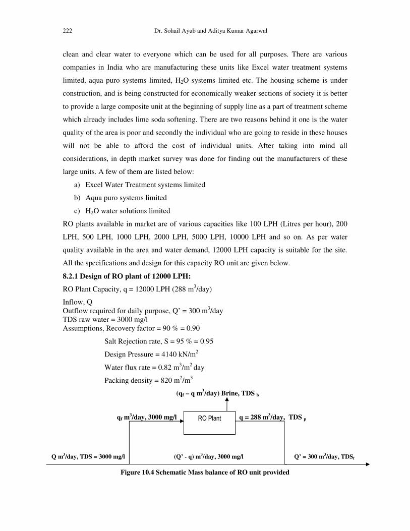
(qf – q m3/day) Brine, TDS b
qf m3/day, 3000 mg/l q = 288 m
3/day, TDS p
Q m
3/day, TDS = 3000 mg/l (Q’ - q) m
3/day, 3000 mg/l Q’ = 300 m
3/day, TDSf
Figure 10.4 Schematic Mass balance of RO unit provided
3 �4� #��
�����������������������������������������������������Design of Water Supply Scheme for …………. 223
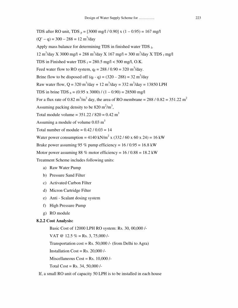
TDS after RO unit, TDS p = [3000 mg/l / 0.90] x (1 – 0.95) = 167 mg/l
(Q’ – q) = 300 – 288 = 12 m3/day
Apply mass balance for determining TDS in finished water TDS f,
12 m3/day X 3000 mg/l + 288 m3/day X 167 mg/l = 300 m3/day X TDS f mg/l
TDS in Finished water TDS f = 280.5 mg/l < 500 mg/l, O.K.
Feed water flow to RO system, qf = 288 / 0.90 = 320 m3/day.
Brine flow to be disposed off (qf - q) = (320 – 288) = 32 m3/day
Raw water flow, Q = 320 m3/day + 12 m3/day = 332 m3/day = 13850 LPH
TDS in brine TDS b = (0.95 x 3000) / (1 – 0.90) = 28500 mg/l
For a flux rate of 0.82 m3/m2 day, the area of RO membrane = 288 / 0.82 = 351.22 m2
Assuming packing density to be 820 m2/m3,
Total module volume = 351.22 / 820 = 0.42 m3
Assuming a module of volume 0.03 m3
Total number of module = 0.42 / 0.03 = 14
Water power consumption = 4140 kN/m2 x (332 / 60 x 60 x 24) = 16 kW
Brake power assuming 95 % pump efficiency = 16 / 0.95 = 16.8 kW
Motor power assuming 88 % motor efficiency = 16 / 0.88 = 18.2 kW
Treatment Scheme includes following units:
a) Raw Water Pump
b) Pressure Sand Filter
c) Activated Carbon Filter
d) Micron Cartridge Filter
e) Anti - Scalant dosing system
f) High Pressure Pump
g) RO module
8.2.2 Cost Analysis:
Basic Cost of 12000 LPH RO system: Rs. 30, 00,000 /-
VAT @ 12.5 % = Rs. 3, 75,000 /-
Transportation cost = Rs. 50,000 /- (from Delhi to Agra)
Installation Cost = Rs. 20,000 /-
Miscellaneous Cost = Rs. 10,000 /-
Total Cost = Rs. 34, 50,000 /-
If, a small RO unit of capacity 50 LPH is to be installed in each house
224 Dr. Sohail Ayub and Aditya Kumar Agarwal
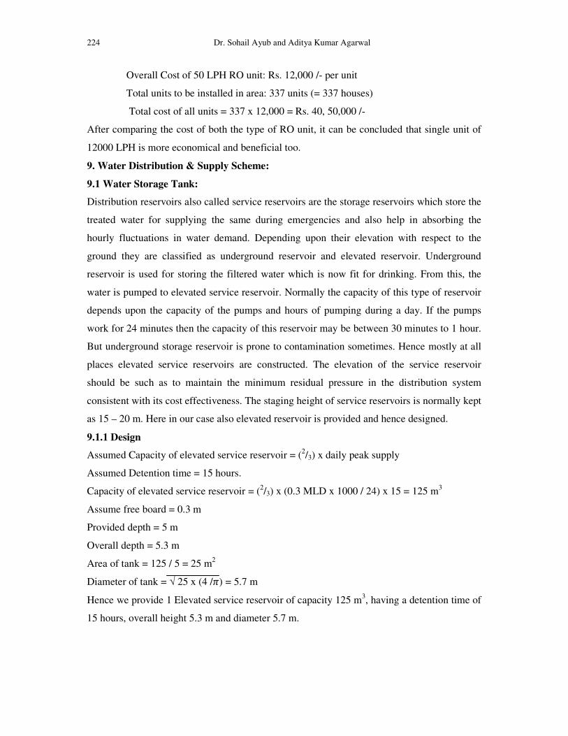
Overall Cost of 50 LPH RO unit: Rs. 12,000 /- per unit
Total units to be installed in area: 337 units (= 337 houses)
Total cost of all units = 337 x 12,000 = Rs. 40, 50,000 /-
After comparing the cost of both the type of RO unit, it can be concluded that single unit of
12000 LPH is more economical and beneficial too.
9. Water Distribution & Supply Scheme:
9.1 Water Storage Tank:
Distribution reservoirs also called service reservoirs are the storage reservoirs which store the
treated water for supplying the same during emergencies and also help in absorbing the
hourly fluctuations in water demand. Depending upon their elevation with respect to the
ground they are classified as underground reservoir and elevated reservoir. Underground
reservoir is used for storing the filtered water which is now fit for drinking. From this, the
water is pumped to elevated service reservoir. Normally the capacity of this type of reservoir
depends upon the capacity of the pumps and hours of pumping during a day. If the pumps
work for 24 minutes then the capacity of this reservoir may be between 30 minutes to 1 hour.
But underground storage reservoir is prone to contamination sometimes. Hence mostly at all
places elevated service reservoirs are constructed. The elevation of the service reservoir
should be such as to maintain the minimum residual pressure in the distribution system
consistent with its cost effectiveness. The staging height of service reservoirs is normally kept
as 15 – 20 m. Here in our case also elevated reservoir is provided and hence designed.
9.1.1 Design
Assumed Capacity of elevated service reservoir = (2/3) x daily peak supply
Assumed Detention time = 15 hours.
Capacity of elevated service reservoir = (2/3) x (0.3 MLD x 1000 / 24) x 15 = 125 m3
Assume free board = 0.3 m
Provided depth = 5 m
Overall depth = 5.3 m
Area of tank = 125 / 5 = 25 m2
Diameter of tank = � 25 x (4 /�) = 5.7 m
Hence we provide 1 Elevated service reservoir of capacity 125 m3, having a detention time of
15 hours, overall height 5.3 m and diameter 5.7 m.
�����������������������������������������������������Design of Water Supply Scheme for …………. 225
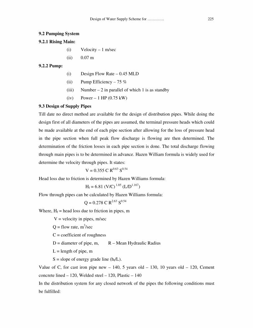
9.2 Pumping System
9.2.1 Rising Main:
(i) Velocity – 1 m/sec
(ii) 0.07 m
9.2.2 Pump:
(i) Design Flow Rate – 0.45 MLD
(ii) Pump Efficiency – 75 %
(iii) Number – 2 in parallel of which 1 is as standby
(iv) Power – 1 HP (0.75 kW)
9.3 Design of Supply Pipes
Till date no direct method are available for the design of distribution pipes. While doing the
design first of all diameters of the pipes are assumed, the terminal pressure heads which could
be made available at the end of each pipe section after allowing for the loss of pressure head
in the pipe section when full peak flow discharge is flowing are then determined. The
determination of the friction losses in each pipe section is done. The total discharge flowing
through main pipes is to be determined in advance. Hazen William formula is widely used for
determine the velocity through pipes. It states:
V = 0.355 C R0.63 S0.54
Head loss due to friction is determined by Hazen Williams formula:
Hf = 6.81 (V/C) 1.85 (L/D1.167)
Flow through pipes can be calculated by Hazen Williams formula:
Q = 0.278 C R2.63 S0.54
Where, Hf = head loss due to friction in pipes, m
V = velocity in pipes, m/sec
Q = flow rate, m3/sec
C = coefficient of roughness
D = diameter of pipe, m, R – Mean Hydraulic Radius
L = length of pipe, m
S = slope of energy grade line (hf/L).
Value of C, for cast iron pipe new – 140, 5 years old – 130, 10 years old – 120, Cement
concrete lined – 120, Welded steel – 120, Plastic – 140
In the distribution system for any closed network of the pipes the following conditions must
be fulfilled:
226 Dr. Sohail Ayub and Aditya Kumar Agarwal
(a) The quantity of water entering a junction must be equal to the quantity of water leaving
the same junction. In other words entering flow must be equal to the leaving flow i.e. law of
continuity is satisfied.
(b) The algebraic sum of the pressure drops around closed loop must be zero i.e. there shall
be continuity in the pressure.
Following are the various methods for the analysis of flow in pipe network
(1) Circle Method
(2) Equivalent Pipe Method
(3) Electrical Analogy Method
(4) Hardy Cross Method
Hardy cross method is most widely used here.
In this method the corrections are applied to the assumed flow in each successive trail. The
head loss in each pipe is determined by pipe flow formula. The successive corrections are
made in the flow in each pipe. The heads are balanced and principle of continuity is satisfied
at each junction.
As per the site plan provided by the Agra development authority, the houses are scattered in
three regions. First region has 255 houses, some single storey, some double storey. Second
region has 65 houses, mostly single storey. Third region has remaining 17 houses, all single
storey. Hence the supply scheme is also designed accordingly. The total flow rate is also
divided into three portions depending upon the ratio of number of houses (water demand is
calculated in these portions depending upon population forecasted similarly as in chapter 2)
in each regions. This also helps in efficient and effective design of pipes using hardy cross
method as loops gets minimized and simplified.
9.3.1 Assumed Flow Rate: a) Region 1 – 227 m3/day
b) Region 2 – 58 m3/day
c) Region 3 – 15 m3/day
Manual design of Supply Pipe by Hardy Cross Method:
a. Material – Cast Iron
b. Main Pipe – Line
i) First Region - Dia. – 150 mm, Length – 200 m, Velocity – 0.15 m/sec
ii) Second Region – Dia. – 150 mm, Length – 500 m, Velocity – 0.04 m/sec
iii) Third Region – Dia. – 100 mm, Length – 1000 m, Velocity – 0.022
m/sec
�����������������������������������������������������Design of Water Supply Scheme for …………. 227
c. Sub – Main Pipe – Line
i) Diameter – 100 mm
ii) Region 1 – Pipe Length – 7000 m, Average Velocity – 0.08 m/sec
iii) Region 2 – Pipe Length – 1450 m, Average Velocity – 0.04 m/sec
10. Conclusion
Water supply scheme for EWS houses in Agra has been designed for a period of 30 years. As
the housing scheme is under construction, the exact population residing in the area and other
data is not known, only data available is that 337 houses are being constructed and their plot
size. So population has been estimated at the rate of 3 persons per house, if the housing
scheme is completed this year itself estimated population in the area will be around 1011
persons. For a design period of 30 years population has been estimated up to the year 2042 by
geometric mean method taking into account population of Agra for the past 5 decades and it
comes out to be 1845. Water demand in the area is calculated as per standard of 135 lpcd
which comes out to be 0.25 MLD and 0.3 MLD after taking into account a peak factor for the
design period. Water available in the area is mostly ground water. Presently, most common
mode of water supply in the area is through bore – well. Water samples were collected from
four different locations around the whole area for laboratory analysis. After conducting
laboratory analysis for various parameters, it was found that water in the area is unsuitable for
drinking purpose and also for various other uses. The results of the analysis were found
unsatisfactory as discussed above. The high range of sulphate, chloride, TDS, alkalinity,
hardness can be attributed to the presence of Sharda Landfill in the vicinity of site. For piped
water supply scheme, this water needs to be treated first before being supplied to houses.
Method of treatment adopted includes softening of water by lime soda softening process and
removal of TDS, sulphate, chloride by reverse osmosis process.
Lime soda softening treatment units includes a chemical storage room of size 10 m by 8.5 m
for storing lime and soda ash, a rapid mixing tank of diameter 0.57 m and depth 1 m for
mixing the chemicals with the help of blades mechanically, circular sedimentation tank of
diameter 3.38 m and depth 3.48 m for settling of flocs formed and a rapid sand gravity filter
of diameter 1.83 m, depth 1.5 m constructed from sand of effective size 0.5 mm for filtering
the water. The total amount of lime and soda ash required for complete treatment of water is
39,456 kg/year lime and 23,020 kg/year soda ash which will cost approximately around Rs. 1,
91,776/- lime/year and Rs. 2, 79,693 soda ash/year. The sludge generated from sedimentation
tank and rapid sand filter is collected in drain pipes and collectively removed by treatment

228 Dr. Sohail Ayub and Aditya Kumar Agarwal
through sludge drying bed. Treated water is further pumped up to the Reverse Osmosis plant
for further treatment. Reverse Osmosis plant has a designed capacity of 12000 LPH (240
m3/day) and contains 14 modules each of individual volume 0.03 m3. Final treated water has
minimum hardness of 40 mg/l, TDS of 285 mg/l.
Treated water is pumped up to an elevated service reservoir (storage tank) for further storage
before final supply. Storage tank of capacity 125 m3, height 5.3 m, diameter 5.7 m is used for
this purpose. A pump of 1 HP is used for pumping treated water to elevated storage reservoir.
Required amount of water is supplied from storage tank with the help of control valves to the
supply pipes. As the houses are scattered in three different regions, so the supply scheme is
also designed accordingly. First region has 255 houses which are supplied with a total 227
m3/day of treated water from storage reservoir through a PVC pipe of diameter 150 mm. This
flow is further supplied accordingly to the houses in this region through the PVC sub main
pipes of diameter 100 mm. Second region has 65 houses which are supplied with 58 m3/day
of treated water from storage reservoir through a PVC pipe of 150 mm. This flow is further
supplied accordingly to the houses in this region through the PVC sub main pipes of
diameter 100 mm. Third region has 17 houses which are supplied with 15 m3/day of treated
water from storage reservoir through a PVC pipe of diameter 100 mm. Here there is no
requirement of sub – main pipe.
As these houses are being constructed for economically weaker sections of society, the water
can directly be supplied through with the help of bore – well pumps as is done by many
people in their houses in general and also those who are living in the vicinity there. This
mode will be less costly as compared to the one which has been discussed here. The initial
plan was same as just mentioned above, but after the results of analysis of water it became
necessary to treat the water before supply and hence a full water supply scheme was designed
for benefit of the people who are going to reside there. People will get safe, clean & clear
water. Coming to the added cost factor for constructing these houses due to the water
treatment & supply scheme, of course people who are going to reside in these houses cannot
afford the cost of it and they don’t need to do it too as they are being provided these houses as
a part of government residential scheme for weaker sections of society and thus the whole
cost should be borne by the government.
�����������������������������������������������������Design of Water Supply Scheme for …………. 229
11. Reference
[1] Central Public Health and Environmental Engineering Organisation (CPHEEO), Ministry
of urban development, Government of India, Manual on water supply and treatment, 1999,
New Delhi.
[2] American Public health Association, Standard methods for examination of water and
wastewater, Washington D.C.
[3] Central Pollution Control Board, Ministry of Environment and Forests, Government of
India, New Delhi, Status of Water Quality in India, 2009.
[4] Murekar N.R., G.H. Raisoni Engineering College, Nagpur, International Journal of
Advanced Engineering Sciences and Technologies, Vol. No. 7, Issue No. 2, 2011, Design of
distribution network of water supply for Kudwa and Katangi-Kala villages.
[5] Jain N.R., S.V.N.I.T, Surat, A project report, Design of water distribution system.
[6] Jain N.R., S.V.N.I.T, Surat, A project report, Design of water treatment plant.
[7] Rode S., Mumbai University, Management research and practice, Vol. 1, Issue 1, 2009,
Equitable Distribution of Drinking water in Municipal corporations in Thane district.
[8] Sinha A.K. and Doshi J., Centre for Technology Alternatives for Rural Areas, IIT
Bombay, 2010, Techno – Economic Feasibility Study Report: Piped Water Supply System
for North Karjat, Maharashtra, India.
[9] Central Pollution Control Board, Ministry of Environment and Forests, Government of
India, New Delhi, Status of Water Treatment Plants in India, 2009.
[10] Central Pollution Control Board, Ministry of Environment and Forests, Government of
India, New Delhi, Status of Water Supply, Wastewater Generation and Treatment in Class – I
Cities and Class – II Towns of India, 2009.
[11] Environmental Engineering: A Book by R.S. Peavy.
[12] Water Works Engineering: A Book by S.R. Qasim.
[13] www.cpcb.nic.in
[14] www.moef.nic.in
[15] www.google.com


![IN AGRA AGRA NAGAR NIGAM, AGRA 1 ekuuh; eq[;ea=h] m0iz0 ekuuh; ea=h] uxj fodkl] m0iz0](https://cdn.vdocuments.us/doc/165x107/55170343550346f5558b5073/in-agra-agra-nagar-nigam-agra-1-ekuuh-eqeah-m0iz0-ekuuh-eah-uxj-fodkl-m0iz0.jpg)


