
.
Control Systems: Classical, Neural, and Fuzzy
Oregon Graduate Institute
Lecture Notes - 1998
Eric A. Wan
1

.
Preface
This material corresponds to the consolidated lecture summaries and handouts for Control
Systems: Classical, Neural, and Fuzzy. The class was motivated from a desire to educate students
interested in neural and fuzzy control. Often students and practitioners studying these subjects
lack the fundamentals. This class attempts to provide both a foundation and appreciation for
traditional control theory, while at the same time, putting newer trends in neural and fuzzy control
into perspective. Yes, this really is only a one quarter class (though not everything was covered
each term). Clearly, the material could be better covered over two quarters and is also not meant
as a substitute for more formal courses in control theory.
The lecture summaries are just that. They are often terse on explanation and are not a substitute
for attending lectures or reading the supplemental material. Many of the summaries were initially
formatted in LaTeX by student1 \scribes" who would try to decipher my handwritten notes after a
lecture. Subsequent years I would try to make minor corrections. Included gures are often copied
directly from other sources (without permission). Thus, these notes are not for general distribution.
This is the rst draft of a working document - beware of typos!
Eric A. Wan
1B. John, M. Kumashikar, Y. Liao, A. Nelson, M. Saell, R. Sharma, T. Srinivasan, S. Tibrewala, X. Tu, S.
Vuuren
i

Contents
Preface i
Class Information Sheet ix
I Introduction 10.1 Basic Structure . . . . . . . . . . . . . . . . . . . . . . . . . . . . . . . . . . . . . . . 1
0.2 Classical Control . . . . . . . . . . . . . . . . . . . . . . . . . . . . . . . . . . . . . . 1
0.3 State-Space Control . . . . . . . . . . . . . . . . . . . . . . . . . . . . . . . . . . . . 2
0.4 Advanced Topics . . . . . . . . . . . . . . . . . . . . . . . . . . . . . . . . . . . . . . 3
0.4.1 Dynamic programming . . . . . . . . . . . . . . . . . . . . . . . . . . . . . . . 3
0.4.2 Adaptive Control . . . . . . . . . . . . . . . . . . . . . . . . . . . . . . . . . . 4
0.4.3 Robust Control / H1 . . . . . . . . . . . . . . . . . . . . . . . . . . . . . . . 4
0.5 History of Feedback Control . . . . . . . . . . . . . . . . . . . . . . . . . . . . . . . . 5
1 Neural Control 6
1.0.1 Reinforcement Learning . . . . . . . . . . . . . . . . . . . . . . . . . . . . . . 7
1.1 History of Neural Networks and Neural Control . . . . . . . . . . . . . . . . . . . . . 9
2 Fuzzy Logic 9
2.1 History . . . . . . . . . . . . . . . . . . . . . . . . . . . . . . . . . . . . . . . . . . . 9
2.2 Fuzzy Control . . . . . . . . . . . . . . . . . . . . . . . . . . . . . . . . . . . . . . . . 10
2.3 Summary Comments . . . . . . . . . . . . . . . . . . . . . . . . . . . . . . . . . . . . 11
II Basic Feedback Principles 12
1 Dynamic Systems - \Equations of Motion" 12
2 Linearization 19
2.1 Feedback Linearization . . . . . . . . . . . . . . . . . . . . . . . . . . . . . . . . . . . 19
2.2 Small Signal Linearization . . . . . . . . . . . . . . . . . . . . . . . . . . . . . . . . . 19
3 Basic Concepts 20
3.1 Laplace Transforms . . . . . . . . . . . . . . . . . . . . . . . . . . . . . . . . . . . . . 20
3.1.1 Basic Properties of Laplace Transforms . . . . . . . . . . . . . . . . . . . . . 20
3.2 Poles and Zeros . . . . . . . . . . . . . . . . . . . . . . . . . . . . . . . . . . . . . . 21
3.3 Second Order Systems . . . . . . . . . . . . . . . . . . . . . . . . . . . . . . . . . . . 22
3.3.1 Step Response . . . . . . . . . . . . . . . . . . . . . . . . . . . . . . . . . . . 23
3.4 Additional Poles and Zeros . . . . . . . . . . . . . . . . . . . . . . . . . . . . . . . . 25
3.5 Basic Feedback . . . . . . . . . . . . . . . . . . . . . . . . . . . . . . . . . . . . . . . 26
3.6 Sensitivity . . . . . . . . . . . . . . . . . . . . . . . . . . . . . . . . . . . . . . . . . . 28
3.7 Generic System Tradeos . . . . . . . . . . . . . . . . . . . . . . . . . . . . . . . . . 30
3.8 Types of Control - PID . . . . . . . . . . . . . . . . . . . . . . . . . . . . . . . . . . 31
3.9 Steady State Error and Tracking . . . . . . . . . . . . . . . . . . . . . . . . . . . . . 33
4 Appendix - Laplace Transform Tables 35
ii
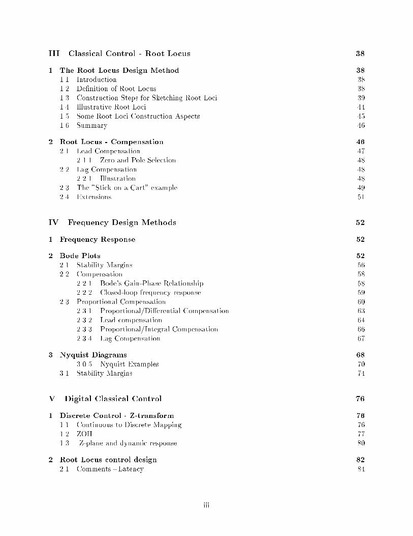
III Classical Control - Root Locus 38
1 The Root Locus Design Method 38
1.1 Introduction . . . . . . . . . . . . . . . . . . . . . . . . . . . . . . . . . . . . . . . . . 38
1.2 Denition of Root Locus . . . . . . . . . . . . . . . . . . . . . . . . . . . . . . . . . . 38
1.3 Construction Steps for Sketching Root Loci . . . . . . . . . . . . . . . . . . . . . . . 39
1.4 Illustrative Root Loci . . . . . . . . . . . . . . . . . . . . . . . . . . . . . . . . . . . 44
1.5 Some Root Loci Construction Aspects . . . . . . . . . . . . . . . . . . . . . . . . . . 45
1.6 Summary . . . . . . . . . . . . . . . . . . . . . . . . . . . . . . . . . . . . . . . . . . 46
2 Root Locus - Compensation 46
2.1 Lead Compensation . . . . . . . . . . . . . . . . . . . . . . . . . . . . . . . . . . . . 47
2.1.1 Zero and Pole Selection . . . . . . . . . . . . . . . . . . . . . . . . . . . . . . 48
2.2 Lag Compensation . . . . . . . . . . . . . . . . . . . . . . . . . . . . . . . . . . . . . 48
2.2.1 Illustration . . . . . . . . . . . . . . . . . . . . . . . . . . . . . . . . . . . . . 48
2.3 The "Stick on a Cart" example . . . . . . . . . . . . . . . . . . . . . . . . . . . . . . 49
2.4 Extensions . . . . . . . . . . . . . . . . . . . . . . . . . . . . . . . . . . . . . . . . . . 51
IV Frequency Design Methods 52
1 Frequency Response 52
2 Bode Plots 52
2.1 Stability Margins . . . . . . . . . . . . . . . . . . . . . . . . . . . . . . . . . . . . . . 56
2.2 Compensation . . . . . . . . . . . . . . . . . . . . . . . . . . . . . . . . . . . . . . . . 58
2.2.1 Bode's Gain-Phase Relationship . . . . . . . . . . . . . . . . . . . . . . . . . 58
2.2.2 Closed-loop frequency response . . . . . . . . . . . . . . . . . . . . . . . . . . 59
2.3 Proportional Compensation . . . . . . . . . . . . . . . . . . . . . . . . . . . . . . . . 60
2.3.1 Proportional/Dierential Compensation . . . . . . . . . . . . . . . . . . . . . 63
2.3.2 Lead compensation . . . . . . . . . . . . . . . . . . . . . . . . . . . . . . . . . 64
2.3.3 Proportional/Integral Compensation . . . . . . . . . . . . . . . . . . . . . . . 66
2.3.4 Lag Compensation . . . . . . . . . . . . . . . . . . . . . . . . . . . . . . . . . 67
3 Nyquist Diagrams 68
3.0.5 Nyquist Examples . . . . . . . . . . . . . . . . . . . . . . . . . . . . . . . . . 70
3.1 Stability Margins . . . . . . . . . . . . . . . . . . . . . . . . . . . . . . . . . . . . . . 74
V Digital Classical Control 76
1 Discrete Control - Z-transform 76
1.1 Continuous to Discrete Mapping . . . . . . . . . . . . . . . . . . . . . . . . . . . . . 76
1.2 ZOH . . . . . . . . . . . . . . . . . . . . . . . . . . . . . . . . . . . . . . . . . . . . . 77
1.3 Z-plane and dynamic response . . . . . . . . . . . . . . . . . . . . . . . . . . . . . . 80
2 Root Locus control design 82
2.1 Comments - Latency . . . . . . . . . . . . . . . . . . . . . . . . . . . . . . . . . . . . 84
iii

3 Frequency Design Methods 84
3.1 Compensator design . . . . . . . . . . . . . . . . . . . . . . . . . . . . . . . . . . . . 84
3.2 Direct Method (Ragazzini 1958) . . . . . . . . . . . . . . . . . . . . . . . . . . . . . 85
4 Z-Transfrom Tables 85
VI State-Space Control 87
1 State-Space Representation 87
1.1 Denition . . . . . . . . . . . . . . . . . . . . . . . . . . . . . . . . . . . . . . . . . . 87
1.2 Continuous-time . . . . . . . . . . . . . . . . . . . . . . . . . . . . . . . . . . . . . . 88
1.3 Linear Time Invariant Systems . . . . . . . . . . . . . . . . . . . . . . . . . . . . . . 88
1.4 "Units" of F in physical terms . . . . . . . . . . . . . . . . . . . . . . . . . . . . . . . 88
1.5 Discrete-Time . . . . . . . . . . . . . . . . . . . . . . . . . . . . . . . . . . . . . . . . 88
1.5.1 Example 2 - "analog computers" . . . . . . . . . . . . . . . . . . . . . . . . . 89
1.6 State Space Vs. Classical Approach . . . . . . . . . . . . . . . . . . . . . . . . . . . 89
1.7 Linear Systems we won't study . . . . . . . . . . . . . . . . . . . . . . . . . . . . . . 90
1.8 Linearization . . . . . . . . . . . . . . . . . . . . . . . . . . . . . . . . . . . . . . . . 91
1.9 State-transformation . . . . . . . . . . . . . . . . . . . . . . . . . . . . . . . . . . . . 92
1.10 Transfer Function . . . . . . . . . . . . . . . . . . . . . . . . . . . . . . . . . . . . . . 92
1.10.1 Continuous System . . . . . . . . . . . . . . . . . . . . . . . . . . . . . . . . . 92
1.10.2 Discrete System . . . . . . . . . . . . . . . . . . . . . . . . . . . . . . . . . . 93
1.11 Example - what transfer function don't tell us. . . . . . . . . . . . . . . . . . . . . . 94
1.12 Time-domain Solutions . . . . . . . . . . . . . . . . . . . . . . . . . . . . . . . . . . . 95
1.13 Poles and Zeros from the State-Space Description . . . . . . . . . . . . . . . . . . . . 98
1.14 Discrete-Systems . . . . . . . . . . . . . . . . . . . . . . . . . . . . . . . . . . . . . . 100
1.14.1 Transfer Function . . . . . . . . . . . . . . . . . . . . . . . . . . . . . . . . . 100
1.14.2 Relation between Continuous and Discrete . . . . . . . . . . . . . . . . . . . . 100
2 Controllability and Observability 101
2.1 Controller canonical form . . . . . . . . . . . . . . . . . . . . . . . . . . . . . . . . . 101
2.2 Duality of the controller and observer canonical forms . . . . . . . . . . . . . . . . . 102
2.3 Transformation of state space forms . . . . . . . . . . . . . . . . . . . . . . . . . . . 102
2.4 Discrete controllability or reachability . . . . . . . . . . . . . . . . . . . . . . . . . . 106
2.4.1 Controllability to the origin for discrete systems . . . . . . . . . . . . . . . . 107
2.5 Observability . . . . . . . . . . . . . . . . . . . . . . . . . . . . . . . . . . . . . . . . 107
2.6 Things we won't prove . . . . . . . . . . . . . . . . . . . . . . . . . . . . . . . . . . . 108
3 Feedback control 109
3.1 Zeros . . . . . . . . . . . . . . . . . . . . . . . . . . . . . . . . . . . . . . . . . . . . . 110
3.2 Reference Input . . . . . . . . . . . . . . . . . . . . . . . . . . . . . . . . . . . . . . . 112
3.3 Selection of Pole Locations . . . . . . . . . . . . . . . . . . . . . . . . . . . . . . . . 114
3.3.1 Method 1 : Dominant second-order poles . . . . . . . . . . . . . . . . . . . . 114
3.3.2 Step Response Using State Feedback . . . . . . . . . . . . . . . . . . . . . . . 115
3.3.3 Gain/Phase Margin . . . . . . . . . . . . . . . . . . . . . . . . . . . . . . . . 117
3.3.4 Method 2 : Prototype Design . . . . . . . . . . . . . . . . . . . . . . . . . . . 119
3.3.5 Method 3 : Optimal Control and Symmetric Root Locus . . . . . . . . . . . . 119
iv

3.4 Discrete Systems . . . . . . . . . . . . . . . . . . . . . . . . . . . . . . . . . . . . . . 127
4 Estimator and Compensator Design 134
4.1 Estimators . . . . . . . . . . . . . . . . . . . . . . . . . . . . . . . . . . . . . . . . . . 134
4.1.1 Selection of Estimator poles e . . . . . . . . . . . . . . . . . . . . . . . . . . 135
4.2 Compensators: Estimators plus Feedback Control . . . . . . . . . . . . . . . . . . . . 136
4.2.1 Equivalent feedback compensation . . . . . . . . . . . . . . . . . . . . . . . . 138
4.2.2 Bode/root locus . . . . . . . . . . . . . . . . . . . . . . . . . . . . . . . . . . 138
4.2.3 Alternate reference input methods . . . . . . . . . . . . . . . . . . . . . . . . 146
4.3 Discrete Estimators . . . . . . . . . . . . . . . . . . . . . . . . . . . . . . . . . . . . . 147
4.3.1 Predictive Estimator . . . . . . . . . . . . . . . . . . . . . . . . . . . . . . . . 147
4.3.2 Current estimator . . . . . . . . . . . . . . . . . . . . . . . . . . . . . . . . . 147
4.4 Miscellaneous Topics . . . . . . . . . . . . . . . . . . . . . . . . . . . . . . . . . . . . 148
4.4.1 Reduced order estimator . . . . . . . . . . . . . . . . . . . . . . . . . . . . . . 148
4.4.2 Integral control . . . . . . . . . . . . . . . . . . . . . . . . . . . . . . . . . . . 148
4.4.3 Internal model principle . . . . . . . . . . . . . . . . . . . . . . . . . . . . . . 149
4.4.4 Polynomial methods . . . . . . . . . . . . . . . . . . . . . . . . . . . . . . . . 149
5 Kalman 150
6 Appendix 1 - State-SpaceControl 151
7 Appendix - Canonical Forms 153
VII Advanced Topics in Control 157
1 Calculus of Variations - Optimal Control 157
1.1 Basic Optimization . . . . . . . . . . . . . . . . . . . . . . . . . . . . . . . . . . . . . 157
1.1.1 Optimization without constraints . . . . . . . . . . . . . . . . . . . . . . . . . 157
1.1.2 Optimization with equality constraints . . . . . . . . . . . . . . . . . . . . . . 157
1.1.3 Numerical Optimization . . . . . . . . . . . . . . . . . . . . . . . . . . . . . . 159
1.2 Euler-Lagrange and Optimal control . . . . . . . . . . . . . . . . . . . . . . . . . . . 159
1.2.1 Optimization over time . . . . . . . . . . . . . . . . . . . . . . . . . . . . . . 159
1.2.2 Miscellaneous items . . . . . . . . . . . . . . . . . . . . . . . . . . . . . . . . 161
1.3 Linear system / ARE . . . . . . . . . . . . . . . . . . . . . . . . . . . . . . . . . . . 161
1.3.1 Another Example . . . . . . . . . . . . . . . . . . . . . . . . . . . . . . . . . . 162
1.4 Symmetric root locus . . . . . . . . . . . . . . . . . . . . . . . . . . . . . . . . . . . . 162
1.4.1 Discrete case . . . . . . . . . . . . . . . . . . . . . . . . . . . . . . . . . . . . 163
1.4.2 Predictive control . . . . . . . . . . . . . . . . . . . . . . . . . . . . . . . . . . 164
1.4.3 Other applied problems . . . . . . . . . . . . . . . . . . . . . . . . . . . . . . 165
2 Dynamic Programming (DP) - Optimal Control 167
2.1 Bellman . . . . . . . . . . . . . . . . . . . . . . . . . . . . . . . . . . . . . . . . . . . 167
2.2 Examples: . . . . . . . . . . . . . . . . . . . . . . . . . . . . . . . . . . . . . . . . . . 168
2.2.1 Routing . . . . . . . . . . . . . . . . . . . . . . . . . . . . . . . . . . . . . . . 168
2.2.2 City Walk . . . . . . . . . . . . . . . . . . . . . . . . . . . . . . . . . . . . . . 168
2.3 General Formulation . . . . . . . . . . . . . . . . . . . . . . . . . . . . . . . . . . . . 168
2.4 LQ Cost . . . . . . . . . . . . . . . . . . . . . . . . . . . . . . . . . . . . . . . . . . . 169
v

2.5 Hamilton-Jacobi-Bellman (HJB) Equations . . . . . . . . . . . . . . . . . . . . . . . 170
2.5.1 Example: LQR . . . . . . . . . . . . . . . . . . . . . . . . . . . . . . . . . . . 171
2.5.2 Comments . . . . . . . . . . . . . . . . . . . . . . . . . . . . . . . . . . . . . . 172
3 Introduction to Stability Theory 173
3.1 Comments on Non-Linear Control . . . . . . . . . . . . . . . . . . . . . . . . . . . . 173
3.1.1 Design Methods . . . . . . . . . . . . . . . . . . . . . . . . . . . . . . . . . . 173
3.1.2 Analysis Methods . . . . . . . . . . . . . . . . . . . . . . . . . . . . . . . . . 173
3.2 Describing Functions . . . . . . . . . . . . . . . . . . . . . . . . . . . . . . . . . . . . 173
3.3 Equivalent gains and the Circle Theorem . . . . . . . . . . . . . . . . . . . . . . . . 175
3.4 Lyapunovs Direct Method . . . . . . . . . . . . . . . . . . . . . . . . . . . . . . . . . 178
3.4.1 Example . . . . . . . . . . . . . . . . . . . . . . . . . . . . . . . . . . . . . . . 180
3.4.2 Lyapunovs Direct Method for a Linear System . . . . . . . . . . . . . . . . . 181
3.4.3 Comments . . . . . . . . . . . . . . . . . . . . . . . . . . . . . . . . . . . . . . 181
3.5 Lyapunovs Indirect Method . . . . . . . . . . . . . . . . . . . . . . . . . . . . . . . . 182
3.5.1 Example: Pendulum . . . . . . . . . . . . . . . . . . . . . . . . . . . . . . . . 182
3.6 Other concepts worth mentioning . . . . . . . . . . . . . . . . . . . . . . . . . . . . . 183
4 Stable Adaptive Control 183
4.1 Direct Versus Indirect Control . . . . . . . . . . . . . . . . . . . . . . . . . . . . . . . 183
4.2 Self-Tuning Regulators . . . . . . . . . . . . . . . . . . . . . . . . . . . . . . . . . . . 184
4.3 Model Reference Adaptive Control (MRAC) . . . . . . . . . . . . . . . . . . . . . . . 185
4.3.1 A General MRAC . . . . . . . . . . . . . . . . . . . . . . . . . . . . . . . . . 187
5 Robust Control 189
5.1 MIMO systems . . . . . . . . . . . . . . . . . . . . . . . . . . . . . . . . . . . . . . . 190
5.2 Robust Stability . . . . . . . . . . . . . . . . . . . . . . . . . . . . . . . . . . . . . . 191
5.2.1 Small gain theorem (linear version) . . . . . . . . . . . . . . . . . . . . . . . . 191
5.2.2 Modeling Uncertainty . . . . . . . . . . . . . . . . . . . . . . . . . . . . . . . 192
5.2.3 Multiplicative Error . . . . . . . . . . . . . . . . . . . . . . . . . . . . . . . . 193
5.3 2-port formulation for control problems . . . . . . . . . . . . . . . . . . . . . . . . . 195
5.4 H1 control . . . . . . . . . . . . . . . . . . . . . . . . . . . . . . . . . . . . . . . . . 196
5.5 Other Terminology . . . . . . . . . . . . . . . . . . . . . . . . . . . . . . . . . . . . . 199
VIII Neural Control 200
1 Heuristic Neural Control 200
1.1 Expert emulator . . . . . . . . . . . . . . . . . . . . . . . . . . . . . . . . . . . . . . 200
1.2 Open loop / inverse control . . . . . . . . . . . . . . . . . . . . . . . . . . . . . . . . 201
1.3 Feedback control - ignoring the feedback . . . . . . . . . . . . . . . . . . . . . . . . . 205
1.4 Examples . . . . . . . . . . . . . . . . . . . . . . . . . . . . . . . . . . . . . . . . . . 205
1.4.1 Electric Arc furnace control . . . . . . . . . . . . . . . . . . . . . . . . . . . . 205
1.4.2 Steel rolling mill . . . . . . . . . . . . . . . . . . . . . . . . . . . . . . . . . . 209
2 Euler-Lagrange Formulation of Backpropagation 213
vi
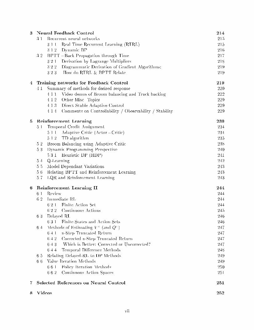
3 Neural Feedback Control 214
3.1 Recurrent neural networks . . . . . . . . . . . . . . . . . . . . . . . . . . . . . . . . . 215
3.1.1 Real Time Recurrent Learning (RTRL) . . . . . . . . . . . . . . . . . . . . . 215
3.1.2 Dynamic BP . . . . . . . . . . . . . . . . . . . . . . . . . . . . . . . . . . . . 216
3.2 BPTT - Back Propagation through Time . . . . . . . . . . . . . . . . . . . . . . . . 217
3.2.1 Derivation by Lagrange Multipliers . . . . . . . . . . . . . . . . . . . . . . . . 218
3.2.2 Diagrammatic Derivation of Gradient Algorithms: . . . . . . . . . . . . . . . 219
3.2.3 How do RTRL & BPTT Relate . . . . . . . . . . . . . . . . . . . . . . . . . 219
4 Training networks for Feedback Control 219
4.1 Summary of methods for desired response . . . . . . . . . . . . . . . . . . . . . . . . 220
4.1.1 Video demos of Broom balancing and Truck backing . . . . . . . . . . . . . . 222
4.1.2 Other Misc. Topics . . . . . . . . . . . . . . . . . . . . . . . . . . . . . . . . . 229
4.1.3 Direct Stable Adaptive Control . . . . . . . . . . . . . . . . . . . . . . . . . . 229
4.1.4 Comments on Controllability / Observability / Stability . . . . . . . . . . . . 229
5 Reinforcement Learning 230
5.1 Temporal Credit Assignment . . . . . . . . . . . . . . . . . . . . . . . . . . . . . . . 234
5.1.1 Adaptive Critic (Actor - Critic) . . . . . . . . . . . . . . . . . . . . . . . . . . 234
5.1.2 TD algorithm . . . . . . . . . . . . . . . . . . . . . . . . . . . . . . . . . . . . 235
5.2 Broom Balancing using Adaptive Critic . . . . . . . . . . . . . . . . . . . . . . . . . 238
5.3 Dynamic Programming Perspective . . . . . . . . . . . . . . . . . . . . . . . . . . . . 240
5.3.1 Heuristic DP (HDP) . . . . . . . . . . . . . . . . . . . . . . . . . . . . . . . . 241
5.4 Q-Learning . . . . . . . . . . . . . . . . . . . . . . . . . . . . . . . . . . . . . . . . . 242
5.5 Model Dependant Variations . . . . . . . . . . . . . . . . . . . . . . . . . . . . . . . 243
5.6 Relating BPTT and Reinforcement Learning . . . . . . . . . . . . . . . . . . . . . . 243
5.7 LQR and Reinforcement Learning . . . . . . . . . . . . . . . . . . . . . . . . . . . . 243
6 Reinforcement Learning II 244
6.1 Review . . . . . . . . . . . . . . . . . . . . . . . . . . . . . . . . . . . . . . . . . . . . 244
6.2 Immediate RL . . . . . . . . . . . . . . . . . . . . . . . . . . . . . . . . . . . . . . . 244
6.2.1 Finite Action Set . . . . . . . . . . . . . . . . . . . . . . . . . . . . . . . . . . 244
6.2.2 Continuous Actions . . . . . . . . . . . . . . . . . . . . . . . . . . . . . . . . 245
6.3 Delayed RL . . . . . . . . . . . . . . . . . . . . . . . . . . . . . . . . . . . . . . . . . 246
6.3.1 Finite States and Action Sets . . . . . . . . . . . . . . . . . . . . . . . . . . . 246
6.4 Methods of Estimating V (and Q) . . . . . . . . . . . . . . . . . . . . . . . . . . . 247
6.4.1 n-Step Truncated Return . . . . . . . . . . . . . . . . . . . . . . . . . . . . . 247
6.4.2 Corrected n-Step Truncated Return . . . . . . . . . . . . . . . . . . . . . . . 247
6.4.3 Which is Better: Corrected or Uncorrected? . . . . . . . . . . . . . . . . . . 247
6.4.4 Temporal Dierence Methods . . . . . . . . . . . . . . . . . . . . . . . . . . . 248
6.5 Relating Delayed-RL to DP Methods . . . . . . . . . . . . . . . . . . . . . . . . . . . 249
6.6 Value Iteration Methods . . . . . . . . . . . . . . . . . . . . . . . . . . . . . . . . . . 249
6.6.1 Policy Iteration Methods . . . . . . . . . . . . . . . . . . . . . . . . . . . . . 250
6.6.2 Continuous Action Spaces . . . . . . . . . . . . . . . . . . . . . . . . . . . . . 251
7 Selected References on Neural Control 251
8 Videos 252
vii

IX Fuzzy Logic & Control 253
1 Fuzzy Systems - Overview 253
2 Sample Commercial Applications 253
3 Regular Set Theory 254
4 Fuzzy Logic 255
4.1 Denitions . . . . . . . . . . . . . . . . . . . . . . . . . . . . . . . . . . . . . . . . . . 255
4.2 Properties . . . . . . . . . . . . . . . . . . . . . . . . . . . . . . . . . . . . . . . . . . 256
4.3 Fuzzy Relations . . . . . . . . . . . . . . . . . . . . . . . . . . . . . . . . . . . . . . . 257
4.4 Boolean Functions . . . . . . . . . . . . . . . . . . . . . . . . . . . . . . . . . . . . . 257
4.5 Other Denitions . . . . . . . . . . . . . . . . . . . . . . . . . . . . . . . . . . . . . . 258
4.6 Hedges . . . . . . . . . . . . . . . . . . . . . . . . . . . . . . . . . . . . . . . . . . . . 258
5 Fuzzy Systems 259
5.1 A simple example of process control. . . . . . . . . . . . . . . . . . . . . . . . . . . . 260
5.2 Some Strategies for Defuzzication . . . . . . . . . . . . . . . . . . . . . . . . . . . . 262
5.3 Variations on Inference . . . . . . . . . . . . . . . . . . . . . . . . . . . . . . . . . . . 262
5.4 7 Rules for the Broom Balancer . . . . . . . . . . . . . . . . . . . . . . . . . . . . . . 264
5.5 Summary Comments on Basic Fuzzy Systems . . . . . . . . . . . . . . . . . . . . . . 264
6 Adaptive Fuzzy Systems 265
6.1 Fuzzy Clustering . . . . . . . . . . . . . . . . . . . . . . . . . . . . . . . . . . . . . . 265
6.1.1 Fuzzy logic viewed as a mapping . . . . . . . . . . . . . . . . . . . . . . . . . 265
6.1.2 Adaptive Product Space Clustering . . . . . . . . . . . . . . . . . . . . . . . . 266
6.2 Additive Model with weights (Kosko) . . . . . . . . . . . . . . . . . . . . . . . . . . 266
6.3 Example Ad-Hoc Adaptive Fuzzy . . . . . . . . . . . . . . . . . . . . . . . . . . . . . 267
6.4 Neuro-Fuzzy Systems . . . . . . . . . . . . . . . . . . . . . . . . . . . . . . . . . . . . 267
6.4.1 Example: Sugene Fuzzy Model . . . . . . . . . . . . . . . . . . . . . . . . . . 268
6.4.2 Another Simple Example . . . . . . . . . . . . . . . . . . . . . . . . . . . . . 269
7 Neural & Fuzzy 269
7.1 NN as design Tool . . . . . . . . . . . . . . . . . . . . . . . . . . . . . . . . . . . . . 270
7.2 NN for pre-processing . . . . . . . . . . . . . . . . . . . . . . . . . . . . . . . . . . . 270
7.3 NN corrective type . . . . . . . . . . . . . . . . . . . . . . . . . . . . . . . . . . . . . 271
7.4 NN for post-processing . . . . . . . . . . . . . . . . . . . . . . . . . . . . . . . . . . . 271
7.5 Fuzzy Control and NN system ID . . . . . . . . . . . . . . . . . . . . . . . . . . . . . 271
8 Fuzzy Control Examples 272
8.1 Intelligent Cruise Control with Fuzzy Logic . . . . . . . . . . . . . . . . . . . . . . . 272
8.2 Fuzzy Logic Anti-Lock Brake System for a Limited Range Coecient of Friction
Surface . . . . . . . . . . . . . . . . . . . . . . . . . . . . . . . . . . . . . . . . . . . . 273
9 Appendix - Fuzziness vs Randomness 275
viii

X Exercises and Simulator 277
HW 1 - Continuous Classical Control 277
HW 2 - Digital Classical Control 277
HW 3 - State-Space 277
HW 4 - Double Pendulum Simulator - Linear SS Control 277
Midterm 277
Double Pendulum Simulator - Neural Control 277
Double Pendulum Simulator Documents 277
0.1 System description for double pendulum on a cart . . . . . . . . . . . . . . . . . . . 278
0.2 MATLAB les . . . . . . . . . . . . . . . . . . . . . . . . . . . . . . . . . . . . . . . 280
ix

ECE553 - Control Systems: Classical, Neural, and Fuzzy
Applications of modern control systems range from advanced aircraft, to processes control in in-
tegrated circuit manufacturing, to fuzzy washing machines. The aim of this class is to integrate
dierent trends in control theory.
Background and perspective is provided in the rst half of the class through review of basic classical
techniques in feedback control (root locus, bode, etc.) as well as state-space approaches (linear
quadratic regulators, Kalman estimators, and introduction to optimal control). We then turn to
more recent movements at the forefront control technology. Articial neural network control is
presented with emphasis on nonlinear dynamics, backpropagation-through-time, model reference
control, and reinforcement learning. Finally, we cover fuzzy logic and fuzzy systems as a simple
heuristic based, yet often eective, alternative for many control problems.
Instructor: Eric A. Wan
Room 581, Phone (503) 690-1164, Internet: [email protected].
Web Page: http://www.ece.ogi.edu/~ericwan/ECE553/
Grading: Homework-45%, Midterm-25%, Project-30%
Prerequisites: Digital signal processing, statistics, MATLAB programming.
Required Text:
1. E. Wan. Control Systems: Classical, Neural, and Fuzzy, OGI Lecture Notes.
Recommended Texts:
(General Control)
1. G. Franklin, J. Powell, M. Workman. Digital Control of Dynamic Systems, 2nd ed. Addison-
Wesley, 1990.
2. G. Franklin, J. Powell, A. Emami-Naeini. Feedback Control of Dynamic Systems, 3rd ed.
Addison-Wesley, 1994.
3. B. Friedland. Control Systems Design: An introduction to state-space methods, McGraw-Hill,
1986
4. C. Phillips, H. Nagle, Digital Control System analysis and design. Prentice-Hall, 1984.
5. B. Shahian, M. Hassul. Control Systems Design Using MATLAB. Prentice Hall, 1993.
6. T. Kailath. Linear Systems. Prentice Hall, 1980
(Optimal Control)
1. A. E. Bryson, Jr., Y. Ho. Applied optimal control : optimization, estimation, and control.
Hemisphere Pub. Corp, 1975.
x

2. M. Edorardo. Optimal, Predictive, and Adaptive Control. Englewood Clis, NJ, Prentice
Hall, 1995.
3. D. Kirk, Optimal Control Theory: An Introduction. Prentice Hall, 1970.
(Adaptive Control)
1. K. S. Narendra, A. M. Annaswamy. Stable adaptive systems. Prentice Hall, 1989.
2. G. Goodwin, K Sin, Adaptive Filtering, Prediction, and Control, Prentice-Hall, 1984.
3. S. Sastry, M. Bodson. Adaptive Control, Stability, Convergence, and Robustness. Prentice
Hall, 1989.
4. K. J. Astrhom, B. Wittenmark. Adaptive Control. Addison-Wesley, 1989.
(Robust / H1 Control)
1. J. C. Doyle, B. A. Francis, A. R. Feedback control theory, Macmillan Pub. Co., 1992.
2. M. Green, D. Limebeer, Linear Robust Control, Prentice Hall, 1995.
(Neural and Fuzzy Control)
1. Handbook of intelligent control : fuzzy, neural, and adaptive approaches, edited by David
A. White, Donald A. Sofge, Van Nostrand Reinhold, 1992. (Strongly recommended but not
required.)
2. Neural Networks for Control, edited by W.T Miller, R. Sutton, P. Werbos. MIT Press, 1991.
3. Reinforcement Learning, R. Sutton, A. Barto, MIT Press, 1998.
4. Neuro-dynamic programming, Dimitri P. Bertsekas and John N. Tsitsiklis, Athena Scientic,
Belmont, 1997.
5. Neurocontrol: Towards An Industry Control Methodology, Tomaas Hrycej, Wiley 1997.
6. B. Kosko, Neural Networks and Fuzzy Systems, Prentice Hall, 1992.
7. Essentials of Fuzzy Modeling and Control, R. Yager, D. Filev, John Wiley and Sons, 1994.
8. E. Cox, The Fuzzy Systems Handbook: A Practitioner's Guide to Building, Using, and Main-
taining Fuzzy Systems, Academic Press, 1994.
9. Fuzzy Logic Technology & Applications, edited by F.J. Marks II, IEEE Press, 1994.
10. F. M. McNeill and E. Thro. Fuzzy Logic: A practical approach, Academic Press, 1994.
11. Fuzzy Sets and Applications, edited by R.R. Yager, John Wiley and Sons, New York, 1987.
xi

Tentative Schedule
Week 1
Introduction, Basic Feedback Principles
Week 2
Bode Plots, Root Locus, Discrete Systems
Week 3
State Space Methods, Pole Placement, Controllability and Observability
Week 4
Optimal Control and LQR, Kalman lters and LQG
Week 5
Dynamic Programming, Adaptive Control or Intro to Robust Control
Week 6
Neural Networks, Neural Control Basics
Week 7
Backpropagation-through-time, Real-time-recurrent learning, Relations to optimal con-
trol
Week 8
Reinforcement Learning, Case studies
Week 9
Fuzzy Logic, Fuzzy Control
Week 10
Neural-Fuzzy, Other
Finals Week
Class Presentations
xii
Part I
Introduction
What is "control"? Make x do y.
Manual control: human-machine interface, e.g., driving a car.
Automatic control (our interest): machine-machine interface (thermostat, moon landing, satel-
lites, aircraft control, robotics control, disk drives, process control, bioreactors).
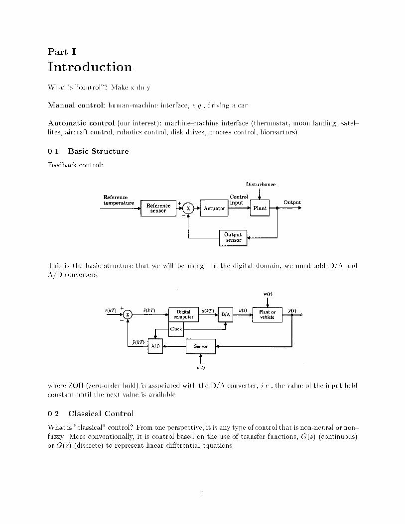
0.1 Basic Structure
Feedback control:
This is the basic structure that we will be using. In the digital domain, we must add D/A and
A/D converters:
where ZOH (zero-order hold) is associated with the D/A converter, i.e., the value of the input held
constant until the next value is available.
0.2 Classical Control
What is "classical" control? From one perspective, it is any type of control that is non-neural or non-
fuzzy. More conventionally, it is control based on the use of transfer functions, G(s) (continuous)
or G(z) (discrete) to represent linear dierential equations.
1

If G(z) = b(z)=a(z), then the roots of a(z) (referred to as poles) and the roots of b(z) (referred to
as zeros), determine the open-loop dynamics. The closed-loop dynamic response of the system is:
y
r=
DG
1 +DG(1)
What is the controller, D(z)? Examples:
k - (proportional control)
ks - (dierential control)
k/s - (integral control)
PID (combination of above)
lead/lag
Classical Techniques:
Root locus
Nyquist
Bode plots
0.3 State-Space Control
State-space, or "modern", control returns to the use of dierential equations:
_x = Ax+ bu (2)
y = Hx (3)
Any linear set of linear dierential equations can be put in this standard form were x is a state-vector.
Control law: given x, control u = kx + r
2

In large part, state-space control design involves nding the control law k. Common methods
include: 1) selecting a desired set of closed loop pole location or 2) optimal control, which involves
the solution of some cost function. For example, the solution of the LQR (linear quadratic regulator)
problem is expressed as the solution of k which minimizesZ1
1
(xTQx+ uTRudt
and addresses the optimal trade-o between tracking performance and control eort.
We can also address issues of:
controllability
observability
stability
MIMO
How to nd the state x? Build an estimator:
with noise (stochastic), we will look at Kalman estimators which yields the LQG (Linear Quadratic
Gaussian)
0.4 Advanced Topics
0.4.1 Dynamic programming
Used to solve for general control law u which minimizes some cost function. This may be used, for
example, to solve the LQR problem, or some nonlinear u = f(x) where the system to be controlled
is nonlinear. Also used for learning trajectory control (terminal control).
Type classes of control problems:
a) Regulators (xed point control) or tracking.
3

b) Terminal control is concerned with getting from point a to point b. Examples: a robotics ma-
nipulator, path-planning, etc.
Terminal control is often used in conjunction with regulator control, where we rst plan an optimal
path and then use other techniques to track that path.
Variations:
a) Model predictive control: This is similar to LQR (innite horizon) but you use a nite horizon
and resolve using dynamic programming at each time step:RN
t0(u2 + Qy2)dt. Also called receding
horizon problem. Popular in process control.
b) Time-optimal control: Getting from point a to point b in minimum time. e.g. solving the opti-
mal trajectory for an airplane to get to a desired location. It is not a steady ascent. The optimal
is to climb to a intermediary elevation, level o, and then swoop to the desired height.
c) Bang-bang control: With control constraints, time-optimal control may lead to bang-bang control
(hard on / hard o).
0.4.2 Adaptive Control
Adaptive control may be used when the system to be controlled is changing with time. May also
be used with nonlinear system when we still want to use linear controllers (for dierent regimes).
In it's basic form, adaptive control is simply gain scheduling: switch in pre-determined control
parameters.
Methods include: self-tuning regulators and model reference control
0.4.3 Robust Control / H1
Robust control deals with the ability of a system to work under uncertainty and encompasses ad-
vanced mathematical methods for dealing with the same. More formally, it minimizes the maximum
singular value of the discrepancies between the closed-loop transfer function matrix and the desired
4

loop shape subject to a closed-loop stability constraint. It is a return to transfer function methods
for MIMO systems while still utilizing state-space techniques.
0.5 History of Feedback Control
Antiquity - Water clocks, level control for wine making etc. (which have now become modern
ush toilets)
1624, Drebble - Incubator (The sensor consisted of a riser lled with alcohol and mercury. A
the re heats up the box, the alcohol expands and the riser oats up lowering the damper on
the ue.)
1728, Watt - Flyball governor
1868, Maxwell - Flyball stability analysis (dierential equations ! linearization ! roots of
\characteristic equation" need be negative). 2nd and 3rd order systems.
1877, Routh - General test for stability of higher order polynomials.
1890, Lyapunov - Stability of non-linear dierential equations (introduced to state-space
control in 1958)
1910, Sperry - Gyroscope and autopilot control
5

1927, Black - Feedback amplier, Bush - Dierential analyzer (necessary for long distance
telephone communications)
1932, Nyquist stability Criterion
1938, Bode - Frequency response methods.
1936 - PID control methods
1942, Wiener - Optimal lter design (control plus stochastic processes)
1947 - Sampled data systems
1948, Evans - Root locus (developed for guidance control of aircraft)
1957, Bellman - Dynamic Programming
1960, Kalman - Optimal Estimation
1960, State-space or \modern" control (this was motivated from work on satellite control,
and was a return to ODE's)
1960's - MIMO state-space control, adaptive control
1980's - Zames, Doyle - Robust Control
1 Neural Control
Neural control (as well as fuzzy control) was developed in part as a reaction by practitioners to the
perceived excessive mathematical intensity and formalism of "classical" control. Although neural
control techniques have been inappropriately used in the past, the eld of neural control is now
starting to mature.
Early systems: open loop: C P1
6

Feedback control with neural networks:
Train by back-propagation-through-time (BPTT) or real-time-recurrent-learning (RTRL).
May have similar objectives and cost functions (as in LQR, minimum-time, model-reference,
etc.) as classical control, but solution are iterative and approximate.
"Approximately optimal control" - optimal control techniques and strategies constrained to
be approximate by nature of training and network architectural constraints.
Often little regard for "dynamics" - few theoretical results regarding stability, controllability,
etc.
Some advantages:
MIMO = SISO
Can handle non-linear systems
Generates good results in many problems
1.0.1 Reinforcement Learning
A related area of neural network control is reinforcement learning ("approximate dynamic program-
ming")
Dynamic programming allows us to do a stepwise cost-minimization in order to solve a more
complicated trajectory optimization. Bellman Optimality Condition: An optimal policy has the
property that whatever the initial state and the initial decision are, the remaining decisions must
constitute an optimal policy with regard to the state resulting from the rst decision.
7

Short-term, or step-wise, maximization of J leads to long term maximization of u(k). (Unfortu-
nately, problems grows exponentially with number of variables).
To minimize some utility function along entire path (to nd control u(k)), need only minimize
individual segments:
J(xk1) = minuk
[r(xk; uk) + J(xk)]
In general, dynamic programming problems can be extremely dicult to solve. In reinforcement
learning, an adaptive critic is used to get an approximation of J.
(These methods are more complicated that other neural control strategies, are hard to train, have
many unresolved issues, but oer great promise for future performance.)
8

1.1 History of Neural Networks and Neural Control
1943, McCoulloch & Pitts - Model of articial neuron
1949, Hebb - simple learning rule
1957, Rosenblatt - Perceptron
1957, Bellman - Dynamic Programming (origins of reinforcement learning, 1960 - Samuel's
learning checker game)
1959, Widrow & Ho - LMS and Adalines (1960 - \Broom Balancer" control)
1967-1982 \Dark Ages"
1983 Barto, Anderson, Sutton - Adaptive Heuristic Critics
1986 Rumelhart, McClelland, et al. - Backpropagation (1974 - Werbos, 1982 - Parker)
1989 Nguyen, Werbos, Jordan, etc. - Backpropagation-Through-Time for control
1990's Increased sophistication, applications, some theory, relation to \classical" control rec-
ognized.
2 Fuzzy Logic
2.1 History
1965, L. Zadeh - Fuzzy Sets
1974, Mamdani & Assilan - Steam engine control using fuzzy logic, other examples.
1980's Explosion of applications from Japan (fuzzy washing machines).
1990's Adaptive Fuzzy Logic, Neural-Fuzzy, etc.
9

2.2 Fuzzy Control
1. No regard for dynamic, stability, mathematical modeling
2. Simple to design
3. Combines heuristic "linguistic" rule-based knowledge with smooth control
4. Elegant "gain scheduling" and interpolation
Fuzzy logic makes use of "membership functions" which introduce an element of ambiguity, e.g.,
the "degree" to which we may consider zero to be zero.
Because of its use of intuitive rules, fuzzy logic can be used appropriately in a wide range of control
problems where mathematical precision is not important, but it is also often misused. Newer
methods try to incorporate ideas from neural networks to adapt the fuzzy systems (neural-fuzzy).
10

2.3 Summary Comments
Classical (and state-space) control is a mature eld that utilizes rigorous mathematics and exact
modeling to exercise precise control over the dynamic response of a system.
Neural control overlaps much with classical control. It is less precise in its formulation yet may
yield better performance for certain applications.
Fuzzy control is less rigorous, but is a simple approach which generates adequate results for many
problems.
There is a place and appropriate use for all three methods.
11

Part II
Basic Feedback Principles
This handout brie y describes some fundamental concepts in Feedback Control.
1 Dynamic Systems - \Equations of Motion"
Where do system equations come from?
Mechanical Systems
12

Rotational Systems
T = I
(Torque) = = (moment of inertia) (angular acceleration)
Satellite
Pendulum
13

\Stick on cart" / Inverted Pendulum (linearized equations)
14

Boeing Aircraft
15

Electrical Circuits
16

Electro-mechanical
Heat Flow
17

Incompressible Fluid Flow
Bio-reactor
18

2 Linearization
Consider the pendulum system shown.
(mg)sinθ
θ
= ml2 +mgl sin (4)
Two methods are typically used in the linear approximation of non-linear systems.
2.1 Feedback Linearization
= mgl sin + u (5)
then,
ml2 = u Linear always! (6)
This method of linearization is used in Robotics for manipulator control.
2.2 Small Signal Linearization
= sin form = g = l = 1: (7)
is a function of and ; f(; ) . Using a Taylors Expansion,
f(; ) = f(0; 0)+@f
@
0;0 + @f
@
0;0
+ : : :higher order terms (8)
f(0; 0) = 0 at equilibrium point.
So, = 0 + ( cos )j0;0 + = +
and for an inverted pendulum
= 0 + ( cos )j0; + = +
These linearized system models should then be tested on the original system to check the accept-
ability of the approximation.
Linearization does not always work, as can be seen from systems below.
Consider the following function _y1 = y31 versus _y2 = y32 ,
19

t
y1
y1
y2
y2
Linearizing both systems yields _yi = 0. However, this is not correct since it would imply that both
systems have similar responses.
3 Basic Concepts
3.1 Laplace Transforms
F (s) =
Z1
0f(t) estdt (9)
The inverse is usually computed by factorization and transformation to the time domain.
f(t) L[ f(t) ]
1 (t)1s
1(t)1s2
t1
s+a eat
1(s+a)2
teat
a
s2+a2
sin ats
s2+a2cosat
s+a(s+a)2+b2
eat cosat
Table 1: Some Standard Laplace Transforms
3.1.1 Basic Properties of Laplace Transforms
Convolution
y(t) = h(t) ? u(t) =
Z1
1
h() u(t )dt (10)
Y (s) = H(s) U(s) (11)
20

Derivatives
_y $ sY (s) y(0) (12)
y(n) + an1y(n1) + : : :+ a1 _y + a0y = bmu
m + bm1um1 + : : :+ b0u (13)
Y (s) =bms
m + bm1sm1 + : : :+ b0
sn + an1sn1 + : : :+ a0U(s) (14)
for y(0) = 0.
Y (s)
U(s)= H(s) =
b(s)
a(s)(15)
H(s) - Transfer Function
Example:
A two mass system represented by two second order coupled equations:
x+b
m1
( _x _y) +k
m1
(x y) = U
m1
y +b
m2
( _y _x) +k
m2
(y x) = 0
s2X(s) +b
m1
(s X(s) s Y (s)) + k
m1
(X(s) Y (s)) = U(s)
m1
s2Y (s) +b
m2
(s Y (s)X(s)) +k
m2
(Y (s)X(s)) = 0
After some algebra we nd that, Y (s)
U(s)= b+ k
(m1s2+b s+ k)(m2s
2+b s+ k) (b+ k)2
3.2 Poles and Zeros
Consider the system,
H(s) =2s+ 1
s2 + 3s+ 2
b(s) = 2 (s+1
2) ! zero :
12
a(s) = (s+ 1) (s+ 2) ! poles : 1;2
21

x x o
H(s) =1s + 1
+3
s + 2; h(t) = et + e2t
The response can be empirically estimated by an inspection of the pole-zero locations. For
stability, poles have to be in the Left half of the s-Plane (LHP). Control is achieved by manipulating
the pole-zero locations.
3.3 Second Order Systems
H(s) =!2n
s2 + 2!ns+ !2n
= damping ratio
!n = natural frequency
s = j!d; = !n; !d = !n
q1 2 (16)
damping = 0 ! oscillation
= 1 ! smooth damping to nal level
1 ! some oscillation; can realize faster response
22

3.3.1 Step Response
Step Response =H(s)
s(17)
y(t) = 1 et(cos!dt+
!dsin!dt) (18)
Rise time : tr 1:8
!n(19)
Overshoot : Mp 1
0:6; 0 0:6 (20)
ts =4:6
(21)
Typical values are :
M = 0:16 for = 0:5
M = 0:4 for = 0:707
23

24

Design Specications
For specied tr , Mp and ts
!n 1:8
tr(22)
0:6 (1Mp) (23)
4:6
ts(24)
for a givenσ for a given
damping ξfor a givenfrequencyω
Pole Locations
3.4 Additional Poles and Zeros
H1(s) =2
(s+ 1)(s+ 2)=
2
s+ 1 2
s+ 2
H2(s) =2(s+ 1:1)
1:1(s+ 1)(s+ 2)=
0:18
s+ 1+
1:64
s+ 2
Here, a zero has been added near one of the poles. The 1.1 factor in the denominator adjusts the
DC gain, as can be seen from the Final Value Theorem :
limt!1
y(t) = lims!0
sY (s) (25)
Note, the zero at -1.1 almost cancels the in uence of the Pole at -1. As s ! 0, the DC gain is
higher by a factor of 1.1, hence the factor in the denominator above.
As Zero approaches origin ! increased overshoot.
Zero in RHP results in non-minimum phase system and a direction reversal in the time
response.
Poles dominated by those nearest the origin.
Poles / Zeros can "cancel" in LHP relative to step response, but may still aect initial
conditions.
25

0 2 4 6 8 10 12 14−0.5
0
0.5
1
1.5
2
2.5
3
3.5
Time (secs)
Am
plitu
de
(zs+1)/(s^2+s+1)
0 5 10 150
0.2
0.4
0.6
0.8
1
1.2
Time (secs)
Am
plitu
de
1/(ps+1)(s^2+s+1)
3.5 Basic Feedback
+r
-
ek H(s)
y
E(s) = R(s) Y (s) (26)
Y (s) = k H(s)E(s) (27)
Y (s) = k H(s) (R(s) Y (s)) (28)
(1 + kH(s))Y (s) = kH(s)R(s) (29)
Y (s)
R(s)=
kH(s)
1 + kH(s);E(s)
R(s)=
1
1 + kH(s)(30)
26

With k large,kH(s)
1 + kH(s)! ;
kH(s)
kH(s)! 1 (31)
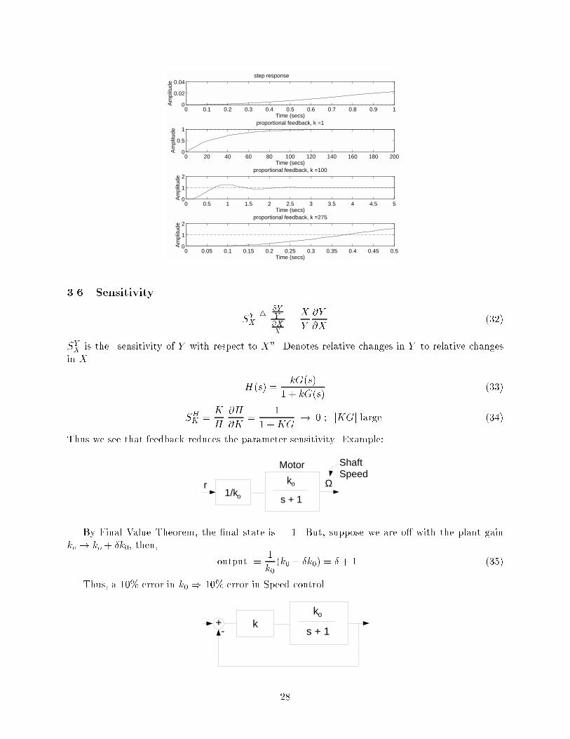
We need to consider the system dynamics. Large k may make the system unstable. Example:
1
s(s+ 2)
The closed loop characteristic equation:
s2 + 2s+ k = 0
x x
0 0.2 0.4 0.6 0.8 1 1.2 1.4 1.6 1.8 20
0.5
1
Time (secs)
Am
plitu
de
step response
0 2 4 6 8 10 12 140
0.5
1
Time (secs)
Am
plitu
de
proportional feedback, k =1
0 0.5 1 1.5 2 2.5 3 3.5 4 4.5 50
1
2
Time (secs)
Am
plitu
de
proportional feedback, k =10
0 0.5 1 1.5 2 2.5 3 3.5 4 4.5 50
1
2
Time (secs)
Am
plitu
de
proportional feedback, k =100
Example 2:
H(s) =1
s [ (s+ 4)2 + 16 ]
The closed loop characteristic equation:
s [ (s+ 4)2 + 16 ] + k = 0
x
.
x
x
27
0 0.1 0.2 0.3 0.4 0.5 0.6 0.7 0.8 0.9 10
0.02
0.04
Time (secs)
Am
plitu
de
step response
0 20 40 60 80 100 120 140 160 180 2000
0.5
1
Time (secs)
Am
plitu
de
proportional feedback, k =1
0 0.5 1 1.5 2 2.5 3 3.5 4 4.5 50
1
2
Time (secs)
Am
plitu
deproportional feedback, k =100
0 0.05 0.1 0.15 0.2 0.25 0.3 0.35 0.4 0.45 0.50
1
2
Time (secs)
Am
plitu
de
proportional feedback, k =275
3.6 Sensitivity
SYX
4
=@Y
Y
@X
X
=X
Y
@Y
@X(32)
SYXis the \sensitivity of Y with respect to X". Denotes relative changes in Y to relative changes
in X
H(s) =kG(s)
1 + kG(s)(33)
SHK=K
H
@H
@K=
1
1 +KG! 0 ; jKGj large (34)
Thus we see that feedback reduces the parameter sensitivity. Example:
r1/k
Ωko
s + 1
Motor ShaftSpeed
o
By Final Value Theorem, the nal state is = 1. But, suppose we are o with the plant gain
ko ! ko + k0, then,
output =1
k0(k0 + k0) = + 1 (35)
Thus, a 10% error in k0 ) 10% error in Speed control.
kko
s + 1+-
28

k k0
s+1
1 + kk0
s+1
=kk0
s + 1 + kk0(36)
Final values =kk0
1 + kk0(37)
Set k2 =1 + kk0
kk0
kko
s + 1+-
rk2
Sensitivity for k0 ! k0 + k0
Final value = k2
k (k0 + k0)
1 + k (k0 + k0)
(38)
k2
24 1
1 + 1k(k0+k0)
35 (39)
1
1 + x 1 x (40)
k2
1 1
k(k0 + k0)
=
1 + kk0
kk0k2
k(k0 + k0) 1
k(k0 + k0)
(41)
= 1 +1
1 + kk0 (42)
for k large ! reduced sensitivity.
Example:
Integral Control
k/sko
s + 1+-
r
kk0
s (s+1)
k
s
k0
s+1+ 1
=k k0
s (s+ 1) + k k0(43)
Final value
29

lim
s! 0 s1
s
kk0
s(s + 1) + kk0
= 1 (44)
0 Steady State Error - Always !
Proportional Control
xfaster
proportional
Increasing k, increases speed of response.
Integral Control
x x
slower responseovershoot
Slower response, but more oscillations.
3.7 Generic System Tradeos
+r
-
e y+
+
D G
γ
ω
µ
For example:
D(s) = +k ; Proportional Control
Y (s) =DG
1 +DGR(s) +
G
1 +DG(s) +
DG1 +DG
(s) (45)
Error
E(s) =1
1 +DGR(s) +
G1 +DG
(s) +1
1 +DG(s) (46)
Disturbance rejectionjDGj 1
30

Good tracking ; E small
jDGj 1
Noise Immunity
jDGj small
3.8 Types of Control - PID
Proportional
D(s) = k ; u(k) = ke(t): (47)
Integral
D(s) =1
Ti
k
s; u(t) =
k
Ti
Zt
0e(t)dt (48)
) Zero steady state error ( may slow down dynamics)
Derivative
D(s) = k TDs (49)
! increases damping and improves stability. Example:
M
damping
G(s) =1
s2 + as
=1
s (s+ a)
x x
31

With derivative
x x
Pole-ZeroCancellation
Closed loop poletrapped here
But what about initial conditions ?
(y) + a ( _y) = u(t)
s2 Y (s) + s y(0) + a s Y (s) + a y(0) = U(s)
Y (s) =s+ a
s(s + a)y(0) +
U(s)
s (s+ a)
+r
-
e yk s
1____s(s+a)+ +
(s+a)Yo Yo/sor
Relative to initial value,
Y (s) =
y(0)
s
1 + k
s+a
limt!1
y(t) = lims!0
s
y(0)
s
1 + k
s+a
! y(0)
1 + k
a
6= 0
Thus, the eect due to initial conditions is not negligible.
PID - Proportional - Integral - Derivative Control
kP + kDs+kI
s
Parameters are often tuned using " Ziegler - Nichols PID tuning"
32

D Ger +
-
y
Figure 1:
3.9 Steady State Error and Tracking
The reference input to a control system is often of the form:
r(t) =tk
k!1(t) (50)
R(s) =1
sk+1(51)
In most cases, the reference input will not be a constant but can be approximated as a linear
function of time for a time span long enough for the system to reach steady state. The error at
this point of time is called the steady-state error.
The type of input to the system depends on the value of k, as follows:
k=0 implies a step input (position)
k=1 implies a ramp input (velocity)
k=2 implies a parabolic input (acceleration)
The steady state error of a feedback control system is dened as:
e14
= limt!1
e(t) (52)
e1 = lims!0
sE(s) (53)
where E(s) is the Laplace transform of the error signal and is dened as:
E(s) =1
1 +D(s)G(s)R(s) (54)
E(s) =1
1 +D(s)G(s)
1
sk+1(55)
e1 = lims!0
1
sk
1
1 +D(s)G(s)
= 0;1; or a constant (56)
Thus, the steady state error depends on the reference input and the loop transfer function.
System Type
The system type is dened as the order k for which e1 is a constant. This also equals number of
open loop poles at the origin. Example:
33

D(s)G(s) =k(1 + 0:5s)
s(1 + s)(1 + 2s)is of type 1 (57)
D(s)G(s) =k
s3is of type 3 (58)
Steady-state error of system with a step-function input (k=0)
Type 0 system:
e1 =1
1+DG(0)==
1
1 +Kp
(59)
where Kp is called the closed loop DC gain or the step-error constant and is dened as:
Kp = lims!0
D(s)G(s) (60)
Type 1 or higher system:
e1 = 0 (61)
(i.e., DG(0) =1, due to pole at origin)
Steady-state error of system with a ramp-function input (k=1)
Type 0 system:
e1 =1 (62)
Type 1 system:
e1 = lims!0
1
s[1 +DG(s)]= lim
s!0
1
sDG(0)==
1
Kv
(63)
where, Kv is called the velocity constant.
Type 2 or higher system:
e1 = 0 (64)
34

4 Appendix - Laplace Transform Tables
35

36

37

Part III
Classical Control - Root Locus
1 The Root Locus Design Method
1.1 Introduction
The poles of the closed-loop transfer function are the roots of the characteristic equation,
which determine the stability of the system.
Studying the behavior of the roots of the characteristic equation will reveal stability and
dynamics of the system, keeping in mind that the transient behavior of the system is also
governed by the zeros of the closed-loop transfer function.
An important study in linear control systems is the investigation of the trajectories of the
roots of the characteristic equation-or, simply, the root loci -when a certain system parameter
varies.
The root locus is a plot of the closed-loop pole locations in the s-plane (or z-plane).
It provides an insightful method for understanding how changes in the gain of the system
feedback in uence the closed loop pole locations.
r e+
-
KD(s) G(s)y
Figure 2:
1.2 Denition of Root Locus
The root locus is dened as a plot of the solution of:
1 + kD(s)G(s) = 0 (65)
We can think of D(s)G(s) as having the following form:
D(s)G(s) =b(s)
a(s)(66)
Then with feedback,kD(s)G(s)
1 + kD(s)G(s)=
kb(s)
a(s) + kb(s)(67)
The zeros of the open loop system do not move.
38

The poles move as a function of k.
The root locus of D(s)G(s) may also be dened as the locus of points in the s-plane where the phase
of D(s)G(s) is 180o. This is seen by noting that 1 + kD(s)G(s) = 0 if kD(s)G(s) = 1, whichimplies that the phase of D(s)G(s) = 180o.
At any point on the s-plane,
6 G = 6 due to zeros 6 due to poles (68)
Example:
For example, consider the open-loop transfer function:
s + 1
s[((s+ 2)2 + 4)(s+ 5)]
The pole-zero plot is shown below:
Assign a test point so = 1 + 2j.
Draw vectors directing from the poles and zeros to the point so.
If so is indeed a point on the root locus, then equation 68 must equal 180o.
6 G = 1 (1 + 2 + 3 + 4)
1.3 Construction Steps for Sketching Root Loci
Step #1: Mark the poles and zeros of the open-loop transfer function.
Step #2: Plot the root locus due to poles on the real axis.
The root locus lies to the left of the odd number of real poles and real zeros.
A single pole or a single zero on the real axis introduces a phase shift of 180o and since
the left half of the s-plane is taken, the phase shift becomes negative.
39

Further, a second pole or a second zero on the real axis will introduce an additional
phase shift of 180o, making the overall phase-shift equal to 360o. Hence, the region is
chosen accordingly.
Here are a few illustrations:
XO
XXO
X
180o
Step #3: Plot the asymptotes of the root loci.
Asymptotes give the behavior of the root loci as k !1.
For 1kG(s) = 0, as k !1, G(s) must approach 0. Typically, this should happen at the
zeros of G(s), but, it could also take place if there are more poles than zeros. We know
that b(s) has order m and a(s) has order n; i.e., let:
b(s)
a(s)=sm + b1s
m1 + :::::
sn + a1sn1 + :::::(69)
So, if n > m then as s!1, G(s)! 0. That is, as s becomes large, the poles and zeros
approx. cancel each other. Thus
1 + kG(s) 1 + k1
(s )nm (70)
=pi zi
n m (71)
where, pi = poles, zi = zeros, and is the centroid.
There are n m asymptotes, where n is the number of zeros and m is the number of
poles, and since 6 G(s) = 180o, we have:
(nm)l = 180o + (l)360o (72)
For instance, nm = 3) l = 60o; 180o; 300o.
The s give the angle where the asymptotes actually go to. Note that the angle of
departure may be dierent and will be looked into shortly.
40

The asymptotes of the root loci intersect on the real axis at and this point of inter-
section is called the centroid. Hence, in other words, the asymptotes are centered at
.
The following gures a few typical cases involving asymptotes (which have the same
appearance as multiple roots):
Step #4: Compute the angles of departure and the angles of arrival of the root
loci. (optional-just use MATLAB)
The angle of departure or arrival of a root locus at a pole or zero denotes the angle of
the tangent to the locus near the point.
The root locus begins at poles and goes either to zeros or to1, along the radial asymp-
totic lines.
To compute the angle of departure, take a test point so very near the pole and compute
the angle of G(so), using equation 72. This gives the angle of departure dep of the
asymptote.
Also, dep = i i 180o 360ol (73)
where, i = sum of the angles to the remaining poles and
i = sum of the angles to all the zeros.
For a multiple pole of order q:
qdep = i i 180o 360ol (74)
In this case, there will be q branches of the locus, that depart from that multiple pole.
41

The same process is used for the angle of arrival arr:
q arr = i i + 180o + 360ol (75)
where, i = sum of angles to all poles, i = sum of all angles to remaining zeros, and
q is the order of the zero at the point of arrival.
Step #5: Determine the intersection of the root loci with the imaginary axis.
(optional)
The points where the root loci intersect the imaginary axis of the s-plane (s = jw),
and the corresponding values of k, may be determined by means of the Routh-Hurwitz
criterion.
A root of the characteristic equation in the RHP implies that the closed-loop system is
unstable, as tested by the R-H criterion.
Using the R-H criterion, we can locate those values of K, for which an incremental
change will cause the number of roots in the RHP to change. Such values correspond to
a root locus crossing the imaginary axis.
Step #6: Determine the breakaway points or the saddle points on the root loci.
(optional)
Breakaway points or saddle points on the root loci of an equation correspond to multiple-
order roots of the equation.
Figure 3: Figure 3(a) illustrates a case in which two branches of the root loci meet at the breakaway
point on the real axis and then depart from the axis in opposite directions. In this case,
the breakaway point represents a double root of the equation, when the value of K is
assigned the value corresponding to the point.
42

Figure 3(b) shows another common situation when two complex-conjugate root loci ap-
proach the real axis, meet at the breakaway point and then depart in opposite directions
along the real axis.
In general, a breakaway point may involve more than two root loci.
Figure 3(c) illustrates such a situation when the breakaway point represents a fourth-
order root.
A root locus diagram can have more than one saddle point. They need not always be
on the real axis and due to conjugate symmetry of root loci, the saddle points not on
the real axis must be in complex-conjugate pairs.
All breakaway points must satisfy the following equations:
dG(s)D(s)
ds= 0 (76)
1 +KG(s)D(s) = 0 (77)
The angles at which the root loci arrive or depart from a saddle point depends on the
number of loci that are involved at the point. For example, the root loci shown in Figures
3(a) and 3(b) all arrive and break away at 180o apart, whereas in Figure 3(c), the four
root loci arrive and depart with angles 90o apart.
In general, n root loci arrive or leave a breakaway point at 180=n degrees apart.
The following gure shows some typical situations involving saddle points.
43

1.4 Illustrative Root Loci
More examples:
X
X
O
O
X
XOX
order 2
XO
X
X
X
XO
order 2
Figure 4:
A MATLAB example:
G(s) =(s+ 3)(s+ 1 j3)
s(s + 1)(s+ 2)3(s+ 4)(s+ 5 2j)(78)
44

Figure 5:
1.5 Some Root Loci Construction Aspects
From the standpoint of designing a control system, it is often useful to learn the eects on the root
loci when poles and zeros of D(s)G(s) are added or moved around in the s-plane. Mentioned below
are a few brief properties pertaining to the above.
Eects of Adding Poles and Zeros to D(s)G(s)
Addition of Poles: In general, adding a pole to the function D(s)G(s) in the left half of the
s-plane has the eect of pushing the root loci toward the right-half plane.
Addition of Zeros: Adding left-half plane zeros to the function D(s)G(s) generally has the
eect of moving and bending the root loci toward the left-half s-plane.
Calculation of gain k from the root locus
Once the root loci have been constructed, the values of k at any point on the loci can be determined.
We know that 1 + kG(s) = 0
kG(s) = 1 (79)
45

k = 1
G(s)(80)
k =1
jG(s)j (81)
Graphically, k =distance from so to zeros
distance from so to poles(82)
1.6 Summary
The Root Locus technique presents a graphical method of investigating the roots of the
characteristic equation of a linear time-invariant system when one or more parameters vary.
The steps of construction listed above should be adequate for making a reasonably adequate
plot of the root-locus diagram.
The characteristic-equation roots give exact indication on the absolute stability of the system.
The zeros of the closed-loop transfer function also govern the dynamic performance of the
system.
2 Root Locus - Compensation
If the process dynamics are of such a nature that a satisfactory design cannot be obtained by a gain
adjustment alone, then some modication of compensation of the process dynamics is indicated.
Two common methods for dynamic compensation are lead and lag compensation.
Compensation with a transfer function of the form
D(s) =s+ zi
s+ pi(83)
is called lead compensation if zi < pi and lag compensation if zi > pi.
Compensation is typically placed in series with the plant in the feedforward path as shown
in the following gure:
Figure 6:
It can also be placed in the feedback path and in that location, has the same eect on the
overall system poles.
46

2.1 Lead Compensation
Lead compensation approximates PD control.
It acts mainly to lower the rise time.
It decreases the transient overshoot, hence improving the system damping.
It raises the bandwidth.
It has the eect of moving the locus to the left.
Illustration: consider a second-order system with transfer function
KG(s) =K
s(s + 1)(84)
G(s) has the root locus shown by the solid line in gure 7. Let D(s) = s+ 2. The root locus
produced by D(s)G(s) is shown by the dashed line. This adds a zero at s = 2. The modied
locus is hence the circle.
Figure 7:
The eect of the zero is to move the root locus to the left, improving stability.
Also, by adding the zero, we can move the locus to a position having closed-loop roots and
damping ratio 0:5
We have "compensated" then dynamics by using D(s) = s+ 2.
The trouble with choosing D(s) based on only a zero is that the physical realization would
contain a dierentiator that would greatly amplify the high-frequency noise present from the
sensor signal. Furthermore, it is impossible to build a pure dierentiator.
Try adding a pole at a high frequency, say at s = 20, to give:
D(s) =s + 2
s+ 20(85)
The following gure shows the resulting root loci when p = 10 and p = 20.
47

Figure 8:
2.1.1 Zero and Pole Selection
Selecting exact values of zi and pi is done by trial and error.
In general, the zero is placed in the neighborhood of the closed-loop control frequency !n.
The pole is located at 3 to 20 times the value of the zero location.
If the pole is too close to the zero, then the root locus moves back too far towards its
uncompensated shape and the zero is not successful in doing its job.
If the pole were too far to the left, then high-frequency noise amplication would result.
2.2 Lag Compensation
After obtaining satisfactory dynamic performance, perhaps by using one or more lead compensators,
the low-frequency gain of the system may be found to be low. This indicates an integration at near-
zero frequencies, and is achieved by lag compensation.
Lag compensation approximates PI control.
A pole is placed near s = 0 (low frequency). But, usually a zero is included near the pole,
so that the pole-zero pair, called a dipole does not signicantly interfere with the dynamic
response of the overall system.
Choose D(s) = s+zs+p
; z > p, where the values of z and p are small (e.g., z = 0:1 and p = 0:01).
Since z > p, the phase is negative, corresponding to a phase lag.
It improves the steady-state error by increasing the low-frequency gain.
Lag compensation however decreases the stability.
2.2.1 Illustration
Again, consider the transfer function, as in equation 84.
Include the lead compensation D1(s) = (s+2)=(s+20) that produced the locus as in gure .
Raise the gain until the closed-loop roots correspond to a damping ratio of = 0:707. At this
point, the root-locus gain is found to be 31.
48

The velocity constant is thus Kv = lims!0 sKDG = (31=10) = 3:1
Now, add a lag compensation of:
D2(s) =s+ 0:1
s + 0:01(86)
This increases the velocity constant by about 10 (since z=p = 10) and keeps the values of
both z and p very small so that D2(s) would have very little eect on the dynamics of the
system. The resulting root locus is as shown in Figure 9.
Figure 9:
The very small circle near the origin is a result of the lag compensation.
A closed-loop root remains very near the lag compensation zero at :1, which will correspondto a very slow decaying transient, which has a small magnitude because the zero will almost
cancel the pole in the transfer function. However, the decay is so slow that this term may
seriously in uence the settling time.
It is thus important to place the lag pole-zero combination at as high a frequency as possible
without causing major shifts in the dominant root locations.
The transfer function from a plant noise to the system error will not have the zero, and thus,
disturbance transients can be very long in duration in a system with lag compensation.
2.3 The "Stick on a Cart" example
mu
O
After normalization, we have: = u (87)
49

) s2(s) (s) = U(s) (88)
(s)
U(s)=
1
s2 1(89)
This results in the following model of the system: The root locus diagram is shown below. The
u θ1/(s^2 - 1)
Figure 10:
X X1-1
Figure 11:
above gure indicates an unstable system, irrespective of the gain.
With lead compensation.
u θe+
-
s + αs + β s -12
1
X XOX
50

The root loci of the lead-compensated system are now in the LHP, which indicates a stable
system.
A slight variation may result in a system as shown below, which may be more satisfactory.
This system may tend to be slower than the one considered above, but may have better
damping.
XXX O
2.4 Extensions
Extensions to Root Locus include time-delays, zero-degree loci, nonlinear functions, etc...
51

Part IV
Frequency Design Methods
1 Frequency Response
Most of this information is covered in the Chapter 5 of the Franklin text.
Frequency domain methods remain popular in spite of other design methods such as root locus,
state space, and optimal control. They can also provide a good design in the face of plant uncer-
tainty in the model.
We start with an open-loop transfer function
Y (s)
U(s)= G(s)! G(jw) (90)
Assume
u(t) = sin(wt) (91)
For a liner system,
y(t) = A sin(wt+ ) (92)
The magnitude is given by
A = jG(jw)j= jG(s)js=jw (93)
And the phase by
= arctanImG(jw)
ReG(jw)= 6 G(jw) (94)
2 Bode Plots
We refer to two plots when we talk about Bode plots
Magnitude plot - log10 magnitude vs. log10w
Phase plot - phase vs. log10w
Given a transfer function in s
KG(s) = K(s+ z1)(s+ z2)(: : :)
(s+ p1)(s+ p2)(: : :)(95)
then there is a corresponding frequency response in jw
KG(jw) = K0(jw1+ 1)(jw2+ 1)(: : :)
(jw)n(jwa + 1)(: : :)(96)
The magnitude plot then shows
log10KG(jw) = log10K0 + log10 jjw1+ 1j+ : : : n log10 jjwj log10 jjwa + 1j : : : (97)
The phase plot shows
6 KG(jw) = 6 K + 6 (jw1+ 1) + : : : n90o 6 (jwa+ 1) : : : (98)
There are three dierent terms to deal with in the previous equations:
52

K(jw)n
(jw + 1)1
(( jwwn)2 + 2 jw
wn+ 1)2
1. K(jw)n
log10Kj(jw)nj = log10K + n log10 jjwj (99)
This term adds a line with slope n through (1,1) on the magnitude plot, and adds a phase of n90to the phase plot. (see gure)
2. (jw + 1)1
When w 1 then the term looks like 1. When w 1 the term looks like jw . This term adds
a line with slope 0 for w < 1and a line with slope 1 for w < 1
to the magnitude plot, and adds
90o of phase when w > 1to the phase plot. (see gures)
3. (( jwwn)2 + 2 jw
wn+ 1)2
This term adds overshoot in the plots. (see gures)
53

54

See gures for sample Bode plots for the transfer function
G(s) =2000(s+ 0:5)
s(s + 10)(s+ 50)(100)
Note that the command BODE in Matlab will create Bode plots given a transfer function.
55

Frequency (rad/sec)
Pha
se (
deg)
; Mag
nitu
de (
dB)
Bode Diagrams
−60
−40
−20
0
20
10−2
10−1
100
101
102
103
−150
−100
−50
2.1 Stability Margins
We can look at the open-loop frequency response to determine the closed-loop stability character-
istics. The root locus plots jKG(s)j = 1 and 6 G(s) = 180o. There are two measures that are used
to denote the stability characteristics of a system. They are the gain margin (GM) and the phase
margin (PM).
The gain margin is dened to be the distance between jKG(jw)j and the magnitude = 1 line
on the Bode magnitude plot at the frequency that satises 6 KG(jw) = 180o. See gures for
examples showing how to determine the GM from the Bode plots. The GM can also be determined
from a root locus plot as
GM =jKj at s = jw
jKj at current design point(101)
The phase margin is dened as the amount by which the phase of G(jw) exceeds 180o at thefrequency that satises jKG(jw)j= 1.
The damping ratio can be approximated from the PM as
PM
100(102)
See gures for examples showing how to determine the PM from the Bode plots. Also, there is a
graph showing the relationship between the PM and the overshoot fraction, Mp. Note that if both
the GM and the PM are positive, then the system is stable. The command MARGIN in Matlab
will display and calculate the gain and phase margins given a transfer function.
56

57

2.2 Compensation
2.2.1 Bode's Gain-Phase Relationship
When designing controllers using Bode plots we should be aware of the Bode gain-phase rela-
tionship. That is, for any stable, minimum phase system, the phase of G(jw) is uniquely determined
by the magnitude of G(jw) (see above). A fair approximation is
6 G(jw) n 90o (103)
where n is the slope of the curve of the magnitude plot. As previously noted, we desire 6 G(jw) >
80o at jKG(jw)j= 1 so a rule of thumb is to adjust the magnitude response so that the slope at
crossover (jKG(jw)j= 1) is approximately -1, which should give a nice phase margin.
Consider the system
G(s) =1
s2(104)
Clearly the slope at crossover = -2. We can use a PD controller
D(s) = K(TDs + 1) (105)
and pick a suitable KandTD = 1w1
to cause the slope at crossover to be -1. Figures below contain
plots of the open-loop and the compensated open-loop Bode plots.
58

2.2.2 Closed-loop frequency response
For the open-loop system, we will typically have
jG(jw)j 1 for w wc , (106)
jG(jw)j 1 for w wc (107)
where wc is the crossover frequency. We can then approximate the closed-loop frequency response
by
jF j = G(jw)
1 +G(jw)
(
1 for w wc
jGj for w wc
(108)
For w = wc, jF j depends on the phase margin. Figure 5.44 shows the relationship of jF j on the
PM for several dierent values for the PM. For a PM of 90o, jF (jwc)j = :7071. Also, if the PM =
90o then bandwidth is equal to wc. There is a tradeo between PM and bandwidth.
59

2.3 Proportional Compensation
60

61

Frequency (rad/sec)
Pha
se (
deg)
; Mag
nitu
de (
dB)
Bode Diagrams
−60
−40
−20
0
20
40
Gm=6.0206 dB (at 1 rad/sec), Pm=21.386 deg. (at 0.68233 rad/sec)
10−1
100
−250
−200
−150
−100
62

2.3.1 Proportional/Dierential Compensation
A PD controller has the form
D(s) = K(TDs + 1) (109)
and can be used to add phase lead at all frequencies above the breakpoint. If no change in gain of
low-frequency asymptote, PD compensation will increase crossover frequency and speed of response.
Increasing frequency-response magnitude at the higher frequencies will increase sensitivity to noise.
The gures below show the eect of a PD controller on the frequency response.
D(s) = K(TDs + 1)
63

2.3.2 Lead compensation
A lead controller has the form
D(s) = KTs+ 1
Ts + 1(110)
where is less than 1. The maximum phase lead then occurs at
w =1pT
(111)
Lead compensation adds phase lead at a frequency band between the two breakpoints, which
are usually selected to bracket the crossover frequency. If no change in gain of low-frequency
asymptote, lead compensation will increase the crossover frequency and speed of response over the
uncompensated system. If gain of low-frequency asymptote is reduced in order not to increase
crossover frequency, the steady-state errors of the system will increase. Lead compensation acts
approximately like a PD compensator, but with less high frequency amplication.
64

An example of lead control is given in the gures. Given an open-loop transfer function
G(s) =1
s(s + 1)(112)
design a lead controller that has a steady-state error of less than 10% to a ramp input. Also the
system is to have and overshoot (Mp) of less than 25%. The steady-state error is given by
e(1) = lims!0
s
1
1 +D(s)G(s)
R(s) (113)
where R(s) = 1s2
for a unit ramp, which reduces to
e(1) = lims!0
8<: 1
s+D(s)[ 1(s+1)
]
9=; =1
D(0)(114)
so we can pick a K = 10. Also, using the relationship between PM and Mp we can see that we
need a PM of 45o to meet the overshoot requirement. We then experiment to nd T and and it
turns out that the desired compensation is
D(s) = 10( s2) + 1
( s
10) + 1
(115)
65

2.3.3 Proportional/Integral Compensation
A PI controller has the form
D(s) =K
s
s +
1
TI
(116)
PI control increases frequency-response magnitude at frequencies below the breakpoint thereby
decreasing steady-state errors. It also contributes phase lag below the breakpoint, which must be
kept at a low enough frequency so that it does not degrade stability excessively. Figures shows how
PI compensation will eect the frequency response.
66

2.3.4 Lag Compensation
A lag controller has the form
D(s) = KTs+ 1
Ts + 1(117)
where is greater than 1. Lag compensation increases frequency-response magnitude at frequencies
below the two breakpoints thereby decreasing steady-state errors. With suitable adjustments in
loop gain, it can alternatively be used to decrease the frequency-response magnitude at frequencies
above the two breakpoints so that the crossover occurs at a frequency that yields an acceptable
phase margin. It also contributes phase lag between the two breakpoints, which must be kept at
low enough frequencies so that the phase decrease does not degrade stability excessively. Figures
show the eect of lag compensation on frequency response.
67

Question: Does increasing gain > 1 or < 1 at 180o cause stability or instability?
Answer: Usually instability, but in some cases the opposite holds. Use root locus or Nyquist
methods to see.
3 Nyquist Diagrams
A Nyquist plot refers to a plot of the magnitude vs. phase, and can be useful when Bode plots are
ambiguous with regard to stability. A Nyquist plot results from evaluating some transfer function
H(s) for values of s dened by some contour (see gures). If there are any poles or zeros inside the
contour then the Nyquist plot will encircle the origin one or more times. The closed-loop transfer
function has the formY
R=
KG(s)
1 +KG(S)(118)
The closed-loop response is evaluated by looking at
1 +KG(S) = 0 (119)
which is simply the open-loop response, KG(s), shifted to the right by 1. Thus 1+KG(S) encircles
the origin i KG(s) encircles 1. We can dene the contour to be the entire RHP (see gures).
If there are any encirclements while evaluating our transfer function, we know that the system is
unstable.
68

A clockwise encirclement of -1 indicates the presence of a zero in the RHP while a counter-
clockwise encirclement of -1 indicate a pole in the RHP. The net # of clockwise encirclements
is
N = Z P (120)
Alternatively, in order to determine whether an encirclement is due to a pole or zero we can
write
1 +KG(s) = 1 +Kb(s)
a(s)=a(s) +Kb(s)
a(s)(121)
So the poles of 1 + KG(s) are also the poles of G(s). Since the number of RHP poles of G(s)
are known, we will assume that an encirclement of -1 indicates an unstable root of the closed-loop
system. Thus we have the number of closed-loop RHP roots
Z = N + P (122)
69

3.0.5 Nyquist Examples
Several examples are given. The rst example has the transfer function
G(s) =1
(s+ 1)2(123)
The root locus shows that the system is stable for all values of K. The Nyquist plot is shown for
K = 1 and it does not encircle 1. Plots could be made for other values of K, but it should be
noted that an encirclement of -1 by KG(s) is equivalent to an encirclement of 1K
by G(s). Since
G(s) only crosses the negative real axis at G(s) = 0, it will never encircle 1K
for positive K.
70

71

The second example has the transfer function
G(s) =1
s(s+ 1)2(124)
and is stable for small values of K. As can be seen from the Nyquist plot, larger values of K will
cause two encirclements. The large arc at innity in the Nyquist plot is due to the pole at 0. Two
poles at s = 0 would have resulted in a full 360o arc at innity.
72

The third example given has the transfer function
G(s) =s+ 1
s( s
10 1)2(125)
For large values of K, there is one counterclockwise encirclement (see gures), so N = 1. But
since P = 1 from the RHP pole of G(s), Z = 0 and there are no unstable system roots. When K
is small, N = 1 which indicates that Z = 2, that there are two unstable roots in the closed-loop
system.
73

3.1 Stability Margins
Now we are interested in dening the gain and phase margins in terms of how far the system is
from encircling the -1 point. The gain margin is dened as the inverse of jKG(jw)j when the plot
crosses the negative real axis. The phase margin is dened to be the dierence between the phase
of G(jw) and 180o when the plot crosses the unit circle. Their determination is shown graphicallyin the gures below. A problem with these denitions is that there may be several GM's and PM's
indicated by a Nyquist plot. A proposed solution is the vector margin which is dened to be the
distance to the -1 point from the closest approach of the Nyquist plot. The vector margin can be
dicult to calculate though.
Recall the denition of sensitivity
S =1
1 +GD(126)
The sensitivity minimized over w is equal to the inverse of the vector margin. A similar result holds
for a MIMO system, where
min1
(S(jw))=
1
kS(jw)k1(127)
where is the maximum singular value of the matrix and k k1 is the innity norm.
74

75

Part V
Digital Classical Control
1 Discrete Control - Z-transform
X(z) =1X
k=1
x(k)zk
Examples
O O O OX XX
X
Step response exponential decay sinusoid
Step response
1(k)! 1
1 z1 Exponential decay
rk ! z
z r sinusoid
[rk cos k]1(k)! z(z r cos )z2 2r(cos )z + r2
For stability ! kpolesk < 1
Final value theorem
limk!1
x(k) = limz!1
(1 z1)X(z)
1.1 Continuous to Discrete Mapping
G(s) G(z)
1. Integration Methods
s z 1
Tforward method
s z 1
Tzbackward method
s 2
T
z 1
z + 1trapezoidal/bilinear transformation method
76

2. Pole-zero mapping
3. ZOH equivalent
D/A G(s) A/Du y
ZOH
sampler (linear & time varying)
(with ant-alias filter)
sample
Gives exact representation between u(k), y(k) (does not necessarily tell you what happens
between samples)
1.2 ZOH
o
o
o
o
o
1
TImpulse- responsesampler - linear, time-variant
Input = 1(t) 1(t T )
Y (s) = (1 eTs)G(s)s
Y (z) = z-transform of samples of y(t)
G(z) = Z fy(kT )g = ZnL1 fY (s)g
o4
= Z fY (s)g for shorthand
= Z
(1 eTs)G(s)
s
= (1 z1)Z
G(s)
s
Example 1:
G(s) =a
s+ a
G(s)
s=
a
s(s+ a)=
1
s 1
s + a
L1G(s)
s
= 1(t) eaT 1(t)
after sampling = 1(kT ) eakT 1(kT )
Z-transform =1
1 z1 1
1 eaT z1 =z(1 eaT )
(z 1)(z eaT )
G(z) =1 eaTz eaT
77

pole at a! pole at eaT , no zero! no zero
Example 2:
G(s) =1
s2
G(z) = (1 z1)Z1
s3
G(z) =
T 2(z + 1)
2(z 1)2Using Table lookup
pole at 0 ! pole at e0T = 1
zero at 1 ! zero at 1
In general,
z = esT for poles
zeros cannot be mapped by the same relationship.
For 2nd order systems - given parameters (Mp; tr; ts; )
The poles s1; s2 = a jb
map to z = rej ; r = eaT ; = bT
smaller the value of T ! closer to the unit circle, i.e. closer to z = 1
Additional comments on ZOH
U(k)! Y (k)
What we really want to control is the continuous output y(t).
Consider sinusoid ! sampled ! ZOH
78

As seen in the gure,
fundamental frequency is still the same
but introduction of phase delay - reduced phase margin (bad for control)
adds higher harmonics.
1 esTs
! s = j! ) ej!T
2 Tsinc(!T
2)
79

As seen in the gure, extra harmonics excite G(s), this may cause aliasing and other eects.
Therefore we need to add an anti-aliasing lter as shown
ZOH G(s)
D/A A/D
anti-alias filter here
1.3 Z-plane and dynamic response
Plot of z = esT for various s:
80

Typically in digital control we can place poles anywhere in the left-half plane, but because of
oscillation, it is preferred to work with positive real part only.
z-plane grid is given by "zgrid" in MATLAB
81

Higher order systems
as pole comes closer to z=1, the system slows down
as zero comes closer to z=1, causes overshoot
as pole and zero come close to each other, they tend to cancel each other
Dead-beat control. In digital domain we can do several things not possible in continuous domain,
e.g. pole-zero cancellation, or suppose we set all closed loop poles to z = 0.
Consider closed loop response
b1z3 + b2z
2 + b3z + b4
z4= b1z
1 + b2z2 + b3z
3 + b4z4
All poles are at 0. This is called dead-beat control.
2 Root Locus control design
2 methods:
1. Emulation
Transform D(s)! D(z)
This is generally considered an older approach.
2. Direct design in the z-domain - The following steps can be followed:
(a)
ZOH + G(s)! G(z)
(b) design specications
Mp; tr; ts ! pole locations in z-domain
(c) Compensator design : Root locus or Bode analysis or Nyquist analysis in Z-domain
82
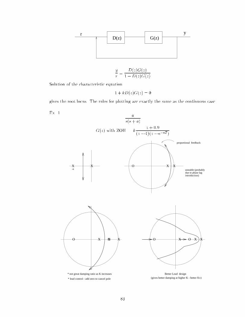
D(z) G(z)r y
y
r=
D(z)G(z)
1 +D(z)G(z)
Solution of the characteristic equation
1 + kD(z)G(z) = 0
gives the root locus. The rules for plotting are exactly the same as the continuous case.
Ex. 1.a
s(s+ a)
G(z) with ZOH = kz + 0:9
(z 1)(z eaT )
XX-a
X XOunstable (probablydue to phase lagintroduction)
proportional feedback
OXO XX
* lead control - add zero to cancel pole
* not great damping ratio as K increases
(gives better damping at higher K - better Kv)
Better Lead design
O X XXO
83

2.1 Comments - Latency
u(k) is a function of y(k) (e.g. lead dierence equation).
computation time (in computer) introduces delay.
Worst case latency - to see the eect of a full 1 clock delay (z1), add a pole at the origin i.e
1/z D(z) G(z)
To overcome this problem we may try to sample faster than required.
sample faster ! complex control
sample slower ! more latency
3 Frequency Design Methods
z = ej!
Rules for construction of Bode plot and Nyquist plots are the same as in continuous domain.
Denitions for GM and PM are the same. However, plotting by \hand" is not practical. (Use
dbode in MATLAB.)
3.1 Compensator design
Proportional k ! k
Derivative ks! k1 z1T
= kz 1
z
PD ! kz z
Integralk
s! k
1 z1
PID D(z) = kp(1 +kdz
z 1+kp(z 1)
z)
84

3.2 Direct Method (Ragazzini 1958)
Closed Loop Response
H(z) =DG
1 +DG
D =1
G(z)
H(z)
1H(z)
Sometimes if H(z) is not chosen properly, D(z) may be non-causal, non-minimal phase or
unstable.
Causal D(z) (cannot have a pole at innity) implies that H(z) must have zero at innity of
the same order as zero of G(z) at innity.
For stability of D(z),
1 - H(z) must contain as zeros, all poles of G(z) that are outside the unit circle
H(z) must contain as zeros all zeros of G(z) that are outside the unit circle
Adding all these constraints to H(z), gives rise to simultaneous equations which are tedious
to solve.
This method is somewhat similar to a method called Pole Placement, though it is not as easy
as one might think. It does not necessarily yield good phase-margin, gain-margin etc. There
are more eective method is State-Space Control.
4 Z-Transfrom Tables
85

86

Part VI
State-Space Control
1 State-Space Representation
Algebraic based method of doing control.
Developed in the 1960's.
Often called \Modern" Control Theory.
Example
f
x
M
f = ma
= mdx2
dt= mx
Let x1 = x (position)
x2 = _x (velocity)
_x1_x2
!=
0 1
0 0
! x1x2
!+
01m
!u
_x = Fx +Gu| z linear in x,u
! state equation
x =
x1x2
!! State
Any linear, nite state, dynamic equation can be expressed in this form.
1.1 Denition
The state of a system at time t0 is the minimum amount of information at t0 that (together with
u(t); t t0) uniquely determines behavior of the system for all t t0.
87

1.2 Continuous-time
First order ODE
_x = f(x; u; t)
y = h(x; u; t)
1.3 Linear Time Invariant Systems
_x = Fx +Gu
y = Hx+ Ju
x(t) Rn (state)
u(t) R (input)
y(t) R (output)
F Rnn
G R1n
H Rn1
J R
Sometimes we will use A;B;C;D instead of the variables F;G;H:J . Note that dimensions change
for MIMO systems.
1.4 "Units" of F in physical terms
1
time= freq
relates derivative of a term to the term
_x = ax, large a ) faster the response.
1.5 Discrete-Time
xk+1 = Fxk +Guk
yk = Hxk + Juk
Sometimes we make use of the following variables,
F ! ;A
G ! ; B
H ! C
J ! D
88

1.5.1 Example 2 - "analog computers"
y + 3 _y y = u
Y (s)
U(s=
1
s2 + 3s 1
Never use dierentiation for implementation.
Instead, use integral model.
-3
1
u y y y
x x x x
..
.. .
1 1 22. .
_x1_x2
!=
3 1
1 0
! x1x2
!+
1
0
!u
y =0 1
x1x2
!
Later we will show standard (canonical) forms for implementing ODE's or TF's.
1.6 State Space Vs. Classical Approach
SS is an internal description of the system whereas Classical approach is an external descrip-
tion.
SS gives additional insight into the control problem and may tell us things about a system
that a TF approach misses (e.g. controllability, observability, internal stability).
Generalizes well to MIMO.
Helps in optimal control design / estimation.
Design
Classical - given specications are natural frequency, damping, rise time, GM, PM
Design a compensator (Lead/Lag PID)
R.L /Bode
find closed loop poleswhich hopefully meet specifications
89

SS - given specications are pole/zero locations or other constraints.
S.S description Exact closed loop poles
iterate on specs to get good GM, PM, etc..
math (place poles)
1.7 Linear Systems we won't study
1.
y(t) = u(t 1)
This simple continuous system of a 1 second delay is innite dimensional.
x(t) = [u(t)]tt1 ( state [0; 1]! R)
t-1 t
u
2. Cantilever beam
y = deflection
u
o
o
u
y
current
voltagetransmission line
Innite dimensional, distributed system, PDE
90
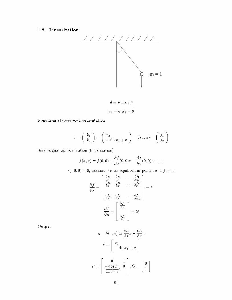
1.8 Linearization
O m = 1
= sin
x1 = ; x2 = _
Non-linear state-space representation.
_x =
_x1_x2
!=
x2 sin x1 + u
!= f(x; u) =
f1f2
!
Small-signal approximation (linearization)
f(x; u) = f(0; 0)+@f
@x(0; 0)x+
@f
@u(0; 0)u+ : : :
(f(0; 0) = 0; assume 0 is an equilibrium point i.e. _x(t) = 0
@f
@x=
2666664@f1
@x1
@f1
@x2: : : @f1
@xn@f2
@x1
@f2
@x2: : : @f2
@xn
......
......
@fn
@x1
@fn
@x2: : :
@fn
@xn
3777775 = F
@f
@u=
2664@f1
@u
...@fn
@u
3775 = G
Output
y = h(x; u) ' @h
@xx +
@h
@uu
_x =
"x2 sin x1 + u
#
F =
264 0 1
cosx1| z 1 or 1
0
375 ; G =
"0
1
#
91

Equilibrium at
x =
0
0
!or
0
!
1.9 State-transformation
ODE ! F;G;H; J
Is x(t) Unique ? NO
Consider,
z = T1x
x = Tz
Given x ! z , z ! x
x, z contain the same amount of information, thus z is a valid state
_x = Fx +Gu
y = Hx+ Ju
_x = T _z = FTz + Gu
_z = T1FT| z A
z + T1G| z B
u
y = HT|zC
z + J|zD
u
There are an innite number of equivalent state-space realizations for a given system
state need not represent physical quantities
T1 =
"1 11 1
#
z =
"1 11 1
# "x1x2
#=
"x1 x2x1 + x2
#
A transformation T may yield an A, B, C, D which may have a "nice" structure even though
z has no physical intuition. We'll see how to nd transformation T later.
1.10 Transfer Function
1.10.1 Continuous System
_X = AX +BU
Y = CX +DU :
Take Laplace-transform:
92
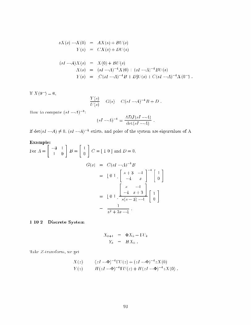
sX(s)X(0) = AX(s) +BU(s)
Y (s) = CX(s) +DU(s)
(sI A)X(s) = X(0)+ BU(s)
X(s) = (sI A)1X(0)+ (sI A)1BU(s)Y (s) = [C(sI A)1B +D]U(s) + C(sI A)1X(0) :
If X(0) = 0,Y (s)
U(s)= G(s) = C(sI A)1B +D :
How to compute (sI A)1:
(sI A)1 = ADJ(sI A)det(sI A) :
If det(sI A) 6= 0, (sI A)1 exists, and poles of the system are eigenvalues of A.
Example:
For A =
"3 1
1 0
#B =
"1
0
#C = [ 1 0 ] and D = 0,
G(s) = C(sI A)1B
= [ 0 1 ]
"s + 3 11 s
#1 "1
0
#
= [ 0 1 ]
"s 11 s + 3
#s(s+ 3) 1
"1
0
#
=1
s2 + 3s 1:
1.10.2 Discrete System
Xk+1 = Xk + Uk
Yk = HXk :
Take Z-transform, we get
X(z) = (zI )1U(z) + (zI )1zX(0)
Y (z) = H(zI )1U(z) +H(zI )1zX(0) :
93

1.11 Example - what transfer function don't tell us.
The purpose of this exercise is to show what transfer functions do not tell us. For the system in
Figures below,
s - 1
s + 11
s - 1
u y
U
s
1 1
s-2
-1 +
X1 X1 X2 X2. .
The state-space equations of the system are as follows:"_x1_x2
#=
"1 0
1 1
# "x1x2
#+
"21
#U
y =h0 1
i " x1x2
#:
Then we have"sx1(s) x1(0)sx2(s) x2(0)
#=
"1 0
1 1
# "x1(s)
x2(s)
#+
"21
#u(s)
x1(s) =1
s+ 1x1(0)
2
s+ 1u(s)
x2(s) =1
s 1[x2(0)
1
2x1(0)] +
1
2(s+ 1)x1(0) +
1
s + 1u(s) :
Take L1-transform,
x1(t) = etx1(0) 2et u(t)y(t) = x2(t)
= et[x2(0)1
2x1(0)] +
1
2etx1(0) + et u(t) :
When t!1, the term et[x2(0) 12x1(0)] goes to 1 unless x2(0) =
12x1(0). The system is uncon-
trollable.
Now consider the system below:
s - 1
s + 1
1
s - 1
u y
94

U YX1 X1 X2 X21
s
1
s+
-2
. .
we have "_x1_x2
#=
"1 0
2 1
# "x1x2
#+
"1
0
#u
y =h1 1
i " x1x2
#
Take L1-transform,
x1(t) = etx1(0) + et u(t)x2(t) = et[x2(0) + x1(0)] etx1(0) + et u(t) et u(t)y(t) = x1(t) + x2(t)
= et(x1(0) + x2(0))+ et u(t)
The system state blows up, but the system output y(t) is stable. The system is unobservable. As
we will see, a simple inspection of A;B;C;D tells us observability or controllability.
1.12 Time-domain Solutions
For a system
_X = AX + BU
Y = CX ;
X(s) = (sI A)1X(0)+ (sI A)1BU(s)Y (s) = CX(s) :
The term (sIA)1X(0) corresponds to the \homogeneous solution", and the term (sIA)1BU(s)is called \particular solution".
Dene the \resolvent matrix" (s) = (sI A)1, then (t) = L1f(sI A)1g, and
X(t) = (t)X(0) +
Zt
0()BU(t )d :
Because
(s) = (sI A)1
=1
s(I A
s)1
=I
s+A
s2+A2
s3+ ;
95

we have
(t) = I + At+(At)2
2!+(At)3
3!+
=1Xk=0
(At)k
k!
= eAt :
Compare the solution of _X = AX with the solution of _x = ax,
X(t) = eAtX(0)
x = eatx(0)
we observed that they have similar format.
To check whether X(t) = eAtX(0) is correct, we calculate deAt=dt
deAt
dt=d(P1
k=0(At)k
k!)
dt= A
1X1
(At)k1
(k 1)!= AeAt :
From above equation and X(t) = eAtX(0), we have
_X =dX
dt= AeAtX(0) = AX :
The matrix exponential eAt has the following properties:
eA(t1+t2) = eAt1 eAt2
e(A+B)t = eAt eBt; only if (AB = BA) :
The conclusion of this section:
X(t) = eAtX(0)+
Zt
0eABU(t )d
Y (t) = CX(t) :
If the matrix A is diagonal, that is
A =
26666641
2
3777775 ;
then
eAt =
2666664e1t
e2t
3777775 ;
If A is not diagonal, we use the following Eqn. to transform A to a diagonal matrix,
= T1AT ;
96

where the columns of T are eigenvectors of A.
Then
eAt = TetT1 :
Example:
For matrix A =
"0 1
0 0
#, (sI A)1 =
"1=s 1=s2
0 1=s
#, we have
eAt = L1f(sI A)1g ="1 t
0 1
#:
Calculating eAt using power series
eAt = I + At+(At)2
2+
=
"1 0
0 1
#+
"0 t
0 0
#+
"0 0
0 0
#+
=
"1 t
0 1
#:
Note: there is no best way to calculate a matrix exponential. A reference is \19 Dubious method
of calculating eAt" by Cleve and Moller.
Consider e100 = 1 100 + 1002
2! 1003
3! + .
State-transition matrices
eFteF (t) = eF (tt) = I
(eFt)1 = eFt :
Thus,
X(t0) = eFt0X(0)
X(0) = eFt0X(to)
X(t) = eFteFt0X(t0)
= eF (tt0)X(t0) :
The eF (tt0) is the state-transition matrix (t ). The last equation relates state at time t0 to
state at time t.
For a time variant system,_X(t) = A(t)X(t) ;
X(t) = (t; t0)X(t0)
@X(t)
@t=
@(t; t0)
@tX(t0)
@(t; t0)
@t= A(t)(t; ) :
97

Because
(t; t) = I
(t3; t1) = (t3; t2)(t2; t1)
I = (t; )(; t) ;
we have
[(t; )]1 = (; t) :
1.13 Poles and Zeros from the State-Space Description
For a transfer function
G(s) =Y (s)
U(s)=b(s)
a(s);
a pole of the transfer function is the \natural frequency", that is the motion of aY for input U 0.
In the state form we have,_X = AX and X(0) = Vi :
Assume X(t) = esitVi, then we have
_X(t) = siesitVi
= AX(t)
= AesitVi :
So,
siVi = AVi ;
that is si is an eigenvalue of A and Vi is an eigenvector of A. We conclude poles = eig(A).
A zero of the system is a value s = si, such that if input u = esitUi, then y 0. For a system in
state form
_X = FX +GU
Y = HX ;
a zero is a value s = si, such that
U(t) = esitU(0)
X(t) = esitX(0)
Y (t) 0 :
Then we have
_X = siesitX(0)
= Fesi tX(0) +GesitU(0) ; orhsi F G
i " X(0)
U(0)
#= 0 :
98

We also have
Y = HX + JU = 0 ; orhH J
i " X(0)
U(0)
#= 0 :
Combine them together, we have"sI F GH J
# "X(0)
U(0)
#=
"0
0
#:
Non-trivial solution exists for det
"sI F GH J
#6= 0. (For mimo systems, look to where this
matrix loses rank.)
The transfer function
G(s) = H(sI F )1G =
det
"sI F GH J
#det[sI F ] :
Example:
For a transfer function
G(s) =s+ 1
(s+ 2)(s+ 3)=
s+ 1
s2 + 5s+ 6:
In state form, the system is
F =
"5 61 0
#
G =
"1
0
#H =
h1 1
i:
The poles of the system are found by solving det[sI F ] = 0, that is
det[sI F ] = det
"s+ 5 6
1 s
#= 0 or
s(s + 5) + 6 = s2 + 5s+ 6 = 0
The zeros of the system are found by solving det
"sI F GH J
#= 0, that is
det
"sI F GH J
#= det
264 s+ 5 6 11 s 0
1 1 0
375= 1(1 s)= s+ 1
99

1.14 Discrete-Systems
1.14.1 Transfer Function
Xk+1 = Xk + Uk
Yk = HXk :
Then
Y (z)
U(z)= H(zI )1 =
det
"zI H 0
#det[zI ]
:
Example: Calculating Xn from X0.
X1 = X0 + U0
X2 = (X0 + U0) + U1
X3 = ((X0 + U0) + U1) + U2
Xn = nX0 +nXi=1
i1Uni
1.14.2 Relation between Continuous and Discrete
ZOH equivalent:
Y(kT)U(kT)ZOH G(s)
G(z)
Figure 12: ZOH
_X = FX + GU
Y = HX + JU
X(t) = eF (tt0)X(t0) +
Zt
t0
eF (t)GU()d :
Let's solve over one sampling period: t = nT + T and t0 = nT , we have
X(nT + T ) = eFTX(nT ) +
ZnT+T
nT
eF (nT+T)GU()d :
100

Because U() = U(nT ) = const for nT nt + T ,
X(nT + T ) = eFTX(nT ) + fZ
nT+T
nT
eF (nT+T)dgGU(nT ) :
Let 2 = nT T , we have
Xn+1 = eFTXn + fZ
T
0eFdgGUn :
So we have
= eFT
= fZ
T
0eFdgG
H $ H
J $ J :
2 Controllability and Observability
2.1 Controller canonical form
Y (s)
U(s)=
b(s)
a(s)=
b1s2 + b2s+ b3
s3 + a1s2 + a2s+ a3
Y (s) = b(s)
U(s)
a(s)
= b(s)(s)
U(s) = a =s3 + a1s
2 + a2s+ a3
(s)
u = (3) + a1 + a2 _ + a3
y = b1 + b2 _ + b3
+
u 1s s
1 1s b3
b2
b1
-a1
-a2
-a3
x1 x2 x3x2 x3
y+
ξ...
ξ ξ ξ.. .
x1. ..
Figure 13:
101

264 _x1_x2_x3
375 =
264 a1 a2 a31 0 0
0 1 0
375| z
Ac
264 x1x2x3
375+264 1
0
0
375| z Bc
u
C =hb1 b2 b3
iD = 0
2.2 Duality of the controller and observer canonical forms
Ac = AT
o
Bc = CT
o
G(s) = Cc(sI Ac)1Bc
G(s) = [Cc(sI Ac)1Bc]
T
BT
c(sI AT
c)1CT
c= Co(sI Ao)
1Bo
Question: Can a canonical form be transformed to another arbitrary form?
A, B, C
A ,B ,C A ,B ,Cc c c o o o
? ?
?
Figure 14:
2.3 Transformation of state space forms
Given F, G, H, J, nd transformation matrix T, such that
A =
264 a1 a2 a31 0 0
0 1 0
375B =
264 1
0
0
375Let
T1 =
264 t1t2t3
375102
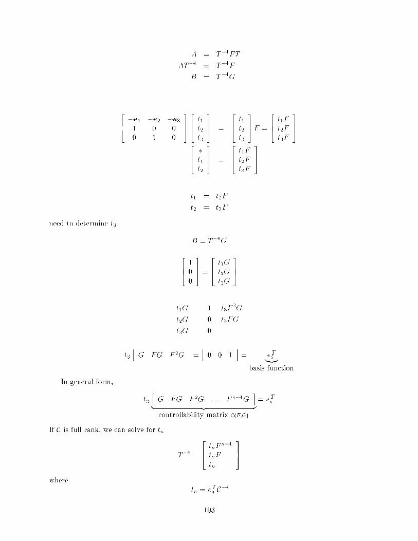
A = T1FT
AT1 = T1F
B = T1G
264 a1 a2 a31 0 0
0 1 0
375264 t1t2t3
375 =
264 t1t2t3
375F =
264 t1F
t2F
t3F
375264 t1t2
375 =
264 t1F
t2F
t3F
375
t1 = t2F
t2 = t3F
need to determine t3
B = T1G
264 1
0
0
375 =
264 t1G
t2G
t3G
375
t1G = 1 = t3F2G
t2G = 0 = t3FG
t3G = 0
t3
hG FG F 2G
i=h0 0 1
i= eT
3|zbasis function
In general form,
tn
hG FG F 2G : : : Fn1G
i| z controllability matrix C(F;G)
= eTn
If C is full rank, we can solve for tn
T1 =
264 tnFn1
tnF
tn
375where
tn = eTn C1
103

Denition: A realization fF;Gg can be converted to controller canonical form i C1(F;G) exists() system is controllable.
corollary: C is full rank () system is controllable
Exercise: Show existence of C1 is unaected by an invertible transformation T, x = Tz.
Bonus question: What's the condition for a system observable?
Given F, G, H, J, solve for Ao; Bo; Co; Do. By duality
Ac = AT
o
Bc = CT
o
i C1(FT ; HT) exists,
hHT FTHT : : : Fn1HT
iT
=
264 H
HF
HFn1
375 = O(F;H)| z observability matrix
Exercise
s - 1
s + 11
s - 1
u y
Figure 15:
F =
"1 0
1 1
#
G =
"21
#
H =h0 1
i
C ="2 2
1 1
#
det(C) = 2 2 = 0 =) not controllable
O =
"0 1
1 1
#
104

det(O) = 1 =) observable
Exercise:
s - 1
s + 1
1
s - 1
u y
Answer: You will get the reverse conclusion to the above exercise.
Conclusion: A pole zero cancellation implies the system is either uncontrollable or unobserv-
able, or both.
Exercise: Show controllability canonical form has C = I =) controllable
Comments
Controllability does not imply observability, observability does not imply controllability.
Given a transfer function,
G(s) =b(s)
a(s)
We can choose any canonical form w like. For example, either controller form or observer
form. But once chosen, we can not necessarily transform between the two.
Redundant states
_x = Fx+ Gu
y = Hx
let xn+1 = Lx
x =
"x
xn+1
#=) unobservability
Denition: A system ( F, G ) is "controllable" if 9 a control signal u to take the states x, from
arbitrary initial conditions to some desired nal state xF , in nite time, () C1exists.
Proof: Find u to set initial conditions
Suppose x(0) = 0 and u(t) = (t)
X(s) = (sI A)1bU(s) = (sI A)1b
I:V:T:= x(0+) = lims!1
sX(s) = lims!1
s(sI A)1b = lims!1
(I A
s)1b = b
Thus an impulse brings the state to b (from 0)
105

Now suppose u(t) = (k)(t)
U(s) = sk
X(s) =1
s(I A
s)1bsk =
1
s(I +
A
s+A2
s2+ : : :)bsk
= bsk1 +Absk2 + : : :+ Ak1b+Akb
s+Ak+1b
s2+ : : :
x(t) = b(k1) +Ab(k2) +Ak1b due to impulse at t=0;
x(0+) = lims!1
sfAkb
s+Ak+1b
s2+ : : :g = Akb
if u(t) = (k)(t)) x(0+) = Akb
Now let
u(t) = g1(t) + g2 _(t) + : : :+ gn(n1)(t), by linearity,
x(0+) = g1b+ g2Ab+ : : :+ gnAn1b =
hb Ab A2b : : : An1b
i264 g1...
gn
375
xdesired = x(0+)
264 g1...
gn
375 = C1x(0+) if C1existsand we can solve for gi to take x(0
+) to any desired vector
Conclusion: We have proven that if a system is controllable, we can instantly move the states
from any given state to any other state, using impulsive inputs. (only if proof is harder )
2.4 Discrete controllability or reachability
A discrete system is reachable i 9 a control signal u that can take the states from arbitrary initial
conditions to some desired state xF , in nite time steps.
xk = Akx0 +kXi=0
Ai1buk1
xN = ANx0 +hb Ab A2b : : : AN1b
i266664u(N 1)
u(N 2)...
u(0)
377775264 u(N 1)
...
u(0)
375 = C1(xd ANx(0))
106
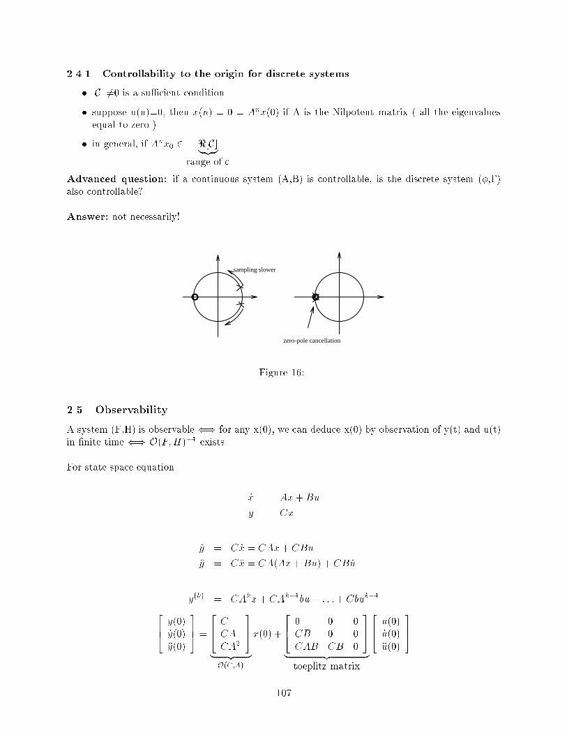
2.4.1 Controllability to the origin for discrete systems
jCj 6=0 is a sucient condition
suppose u(n)=0, then x(n) = 0 = Anx(0) if A is the Nilpotent matrix ( all the eigenvalues
equal to zero ).
in general, if Anx0 2 <[C]|zrange of C
Advanced question: if a continuous system (A,B) is controllable, is the discrete system (,)
also controllable?
Answer: not necessarily!
zero-pole cancellation
sampling slower
Figure 16:
2.5 Observability
A system (F,H) is observable () for any x(0), we can deduce x(0) by observation of y(t) and u(t)
in nite time () O(F;H)1 exists
For state space equation
_x = Ax+ Bu
y = Cx
_y = C _x = CAx+ CBu
y = Cx = CA(Ax+ Bu) + CB _u
...
y(k) = CAkx+ CAk1bu+ : : :+ Cbuk1264 y(0)
_y(0)
y(0)
375 =264 C
CA
CA2
375| z O(C;A)
x(0) +
264 0 0 0
CB 0 0
CAB CB 0
375| z toeplitz matrix
264 u(0)
_u(0)
u(0)
375
107

x(0) = O1(A;C)
8><>:264 y(0)
...
yn1
375 T264 u(0)
...
un1(0)
3759>=>;
if O1exists, we can deduce x(0)
Exercise: solve for discrete system
x(k) = O1264 y(k)
...
y(k+ n 1)
375+ T
264 u(k)...
u(k + n 1)
3752.6 Things we won't prove
If A;B;C is observable and controllable, then it is minimal, i.e, no other realization has a
smaller dimension). This implies a(s) and b(s) are co-prime.
The unobservable space
N (O) = fx 2 RnjOx = 0g is the null space of O
solutions of _x = Ax which start in unobservable space cannot be seen by looking at output
(i.e. we stay in unobservable space).
If x(0) 2 N (O), then y = Cx = 0 for all t.
The controllable space,
<(C) = fx = Cvjv 2 Rng is the range space of C
If x(0) 2 <(C) and _x = Ax + Bu , then, x(t) 2 <(C)8 t for any u(t) )the control can only
move the state in <(C)
PBH(Popov-Belevitch-Hautus ) Rank Tests
1. A system f A, B g is controllable i rank [sI-A b]=N for all s.
2. A system f A, C g is observable i
rank
"C
sI A
#= N for all s.
3. These tests tell us which modes are uncontrollable or unobservable.
Grammian Tests
P (T; t) =
ZT
t
(T; )B()B0
()0
(T; )d, where is the state transition matrix.
A system is controllable i P(T,t) is non singular for some T>t. For time invariant system,
P (T ) =
ZT
0eAtBBT eAtdt
108
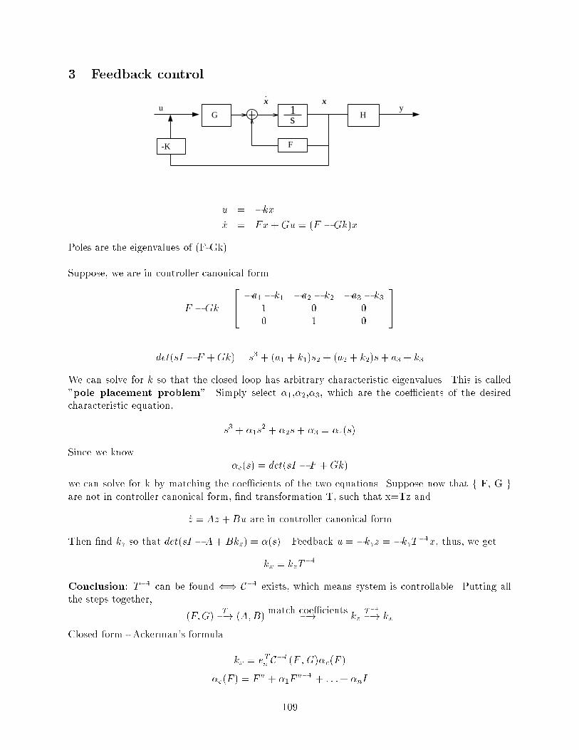
3 Feedback control
uG H
F-K
y1s
x x.
u = kx_x = Fx+ Gu = (F Gk)x
Poles are the eigenvalues of (F-Gk).
Suppose, we are in controller canonical form
F Gk =
264 a1 k1 a2 k2 a3 k31 0 0
0 1 0
375
det(sI F +Gk) = s3 + (a1 + k1)s2 + (a2 + k2)s+ a3 + k3
We can solve for k so that the closed loop has arbitrary characteristic eigenvalues. This is called
"pole placement problem". Simply select 1,2,3, which are the coecients of the desired
characteristic equation,
s3 + 1s2 + 2s+ 3 = c(s)
Since we know
c(s) = det(sI F + Gk)
we can solve for k by matching the coecients of the two equations. Suppose now that f F, G gare not in controller canonical form, nd transformation T, such that x=Tz and
_z = Az +Bu are in controller canonical form
Then nd kz so that det(sI A+ Bkz) = (s) . Feedback u = kzz = kzT1x, thus, we get
kx = kzT1
Conclusion: T1 can be found () C1 exists, which means system is controllable. Putting all
the steps together,
(F;G)T! (A;B)
match coecients! kzT1
! kx
Closed form - Ackerman's formula
kx = eTnC1 (F ;G)c(F )
c(F ) = Fn + 1Fn1 + : : :+ nI
109
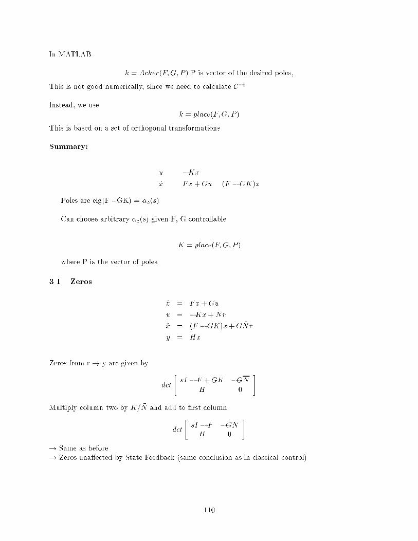
In MATLAB
k = Acker(F;G; P ) P is vector of the desired poles,
This is not good numerically, since we need to calculate C1.
Instead, we use
k = place(F;G; P )
This is based on a set of orthogonal transformations.
Summary:
u = Kx_x = Fx + Gu = (F GK)x
Poles are eig(F - GK) = c(s).
Can choose arbitrary c(s) given F, G controllable.
K = place(F;G; P )
where P is the vector of poles.
3.1 Zeros
_x = Fx +Gu
u = Kx+ Nr
_x = (F GK)x+G Nr
y = Hx
Zeros from r ! y are given by
det
"sI F +GK GN
H 0
#
Multiply column two by K= N and add to rst column.
det
"sI F G N
H 0
#! Same as before
! Zeros unaected by State Feedback (same conclusion as in classical control)
110

Example :
G(s) =(s+ 2)(s 3)
s3 + s 10
Set c(s) = (s+ 1)(s+ 2)(s 3)
C(sI A+ GK)1B =1
s+ 1
! unobservable
Does it aect controllability ? No
F GK ! still in Controller Canonical Form.
Example
_x =
"1 1
0 2
#x+
"1
0
#u
det(sI A+ BK) =
s 1 + k1 1 + k20 s 2
= (s 1 + k1) (s 2)| z uncontrollable mode
= +2 check with PBH
Example
X
_x = x+ u
u = Kx_x = (1 +K)x
x(t) = e(1+K)t; x(0) = 1
u = ke(1+K)t; x(0) = 1
111

larger K
As K ! 1 (large gain), u looks more and more like (t) which instantaneously moves x to
0. (recall proof for controllability)
3.2 Reference Input
_x = Fx+ Gu
y = Hx
r = ref
1. Assume r ! constant as t !1 (e.g. step)
2. Want y ! r as t ! 1
Let,
u = K(x xss) + uss
xss = Nxr
uss = Nur
-K
Nx
Nur
x
-
+
+
r+N
-K
F,G,H
x
u
112

N = (KNx +Nu)
At steady state,
x ! xss
_x ! 0
u ! uss
0 = Fxss + Guss
yss = Hxss = r
FNxr +GNur = 0
HNxr = r
Divide by r. "F G
H 0
#"Nx
Nu
#=
"0
1
#
"Nx
Nu
#=
"F G
H 0
#1 "
0
1
#
Example: Two mass system
M1 M2
X1 X2
We know, that in steady state 26664x1_x1x2_x2
37775!266641
0
1
0
37775
Hence,
Nx =
266641
0
1
0
37775 ; and Nu = 0
113

Nx; Nu more robust - Independent of M1;M2 In contrast, N = (KNx +Nu)! changes with K.
For SISO systems
y
r= H(sI F + GK)1GN
G(s) js=0= 1 =) N =1
H(F + GK)1G
3.3 Selection of Pole Locations
Suppose F, G are controllable, where should the poles be placed? There are three common methods
for placing the poles.
3.3.1 Method 1 : Dominant second-order poles
y
r=
!2n
s2 + 2!ns + !2n
Example
1 .1
slinky
XXXX
X
X
-.014 + 1.0003
Choose 2nd order dominant pole locations:
!n = 1
= 0:5
c = s2 + s+ 1
pd =12p3
2i
114

Take other 2 poles to be
!n = 4; = 0:5; (4 pd)
p =
0BBB@1=2 +
p3i=2
1=2p3i=2
2 + 2p3i
2 2p3i
1CCCAMATLAB:
K = place(F;G; P )
K = [19:23 4:96 1:6504 16:321]
eort is the price of moving poles.
3.3.2 Step Response Using State Feedback
N G H
-F
-K
r u + 1/s
y
_x = Fx +Gu
u = Kx+ Nr
y = Hx
_x = (F GK)x+ NGr
where N is a scale factor.
MATLAB:
y = step(F GK;NG;H; 0; 1; t)
Example
% MATLAB .m file for Two Mass System. State Feedback, E. Wan
% Parameters
M = 1
m = .1
115

k = 0.091
b = 0.0036
% State-Space Description
F = [0 1 0 0; -k/M -b/M k/M b/M ;0 0 0 1; k/m b/m -k/m -b/m]
G = [0 1/M 0 0]'
H = [0 0 1 0]
J = 0
% Desired pole locations
Pd = roots([1 1 1])
P = [Pd 4*Pd]
K = place(F,G,P)
% Closed loop pole locations
pc = eig(F-G*K)
% Reference Design
Nx = [1 0 1 0]';
Nb = K*Nx
% Step Response
t = 0:.004:15;
subplot(211)
[Y,X] = step(F-G*K,G*Nb,H,0,1,t);
plot(t,H*X','--');
subplot(212)
plot(t,-K*X'+Nb,'--');
title('2-Mass control ref. step')
% Standard Root Locus vs Plant Gain
%axis('square');
%rlocus(F,G,K,0)
%title('Plant/State-Feedback Root Locus')
%rcl = rlocus(F,G,K,0,1)
%hold
%plot(rcl,'*')
%axis([-4 4 -4 4]);
% Bode plot of loop transfer function
%margin(F,G,K,0)
116
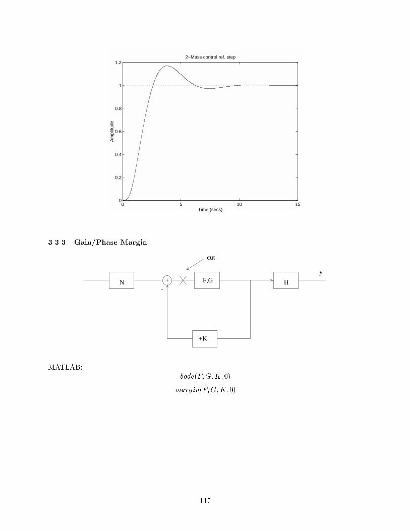
0 5 10 150
0.2
0.4
0.6
0.8
1
1.2
Time (secs)
Am
plitu
de
2−Mass control ref. step
3.3.3 Gain/Phase Margin
N H+ F,G
+K
cut
-
y
MATLAB:
bode(F;G;K; 0)
margin(F;G;K; 0)
117

10−1
100
101
−100
0
100
Frequency (rad/sec)
Gai
n dB
Gm=−51.45 dB, (w= 1.006) Pm=52.22 deg. (w=5.705)
10−1
100
101
0
−90
−180
−270
−360
Frequency (rad/sec)
Pha
se d
eg
Root Locus
MATLAB:
rlocus(F;G;K; 0)
−4 −3 −2 −1 0 1 2 3 4−4
−3
−2
−1
0
1
2
3
4
Real Axis
Imag
Axi
s
Plant/State−Feedback Root Locus
Open loop (F;G;H)
Closed loop (F GK;NG;H)
118

Open loop for stability check
(F;G;K)
T:F: = K(sI F )1G
3.3.4 Method 2 : Prototype Design
Select prototype responses with desirable dynamics. There are several sets of these -
Butterworth1
1 + (!=!o)2n
Bessel
ITAE: Minimizes the Integral of the Time multiplied by the Absolute value of Error,
J =
Zt
0t j e j dt
e
(35 years ago - by twiddling and trial and error)
All these methods set pole locations and ignore the in uence of plant zeros.
3.3.5 Method 3 : Optimal Control and Symmetric Root Locus
Suppose we want to minimize
J =
Z1
0e2dt
Optimal Control Law for this is a bunch of 's and its derivatives. But the 's are not practical.
Linear Quadratic Constraints
J =
Ztf
0
hxT (t)Qx(t) + uT (t)Ru(t)
idt + xT (tf )Sx(tf)
where Q, R and S are positive denite weighting matrices. x ! 0 is equivalent to e ! 0.
It turns out that
u(t) = K(t)x(t)
which is time varying state control.
119

The linear feedback K(t) may be solved through Dynamic Programming (next chapter).
A general \optimal" control has the form.
J =
Ztf
0[L(x; u; t)]dt+ L2(x(tf); u(tf))
which may be dicult to solve. For the special case
J =
Z1
0
hxTQx+ uTRu
idt
we have the Linear Quadratic Regulator.
and
u = kx =) xed feedback control.
SRL
Q = 2HTH
R = I
=) J =
Z1
0
h2y2 + u2
idt
Solution of u = Kx leads to the optimal value of K, which places the closed loop poles at the
stable roots of the equation,
1 + 2GT (s)G(s) = 0 where G(s) =Y (s)
U(s)(open loop)
This is called the Symmetric Root Locus. The locus in the LHP has a mirror image in the RHP.
The locus is symmetric with respect to the imaginary axis.
= 0 : expensive control, since control eort has to be minimized
= 1 : cheap control, since y2 has to be minimized, hence actuators may approach delta
functions.
Examples
G(s) =1
s2
G(s) =1
(s)2 =1
s2
120

X4
Example: Two Mass system
X
X
X
X
O OXXXX
MATLAB :
K = LQR(F;G;Q;R)
where
Q = 2HTH
R = I
% MATLAB .m file for Two Mass System. LQR State Feedback, E. Wan
% Parameters
M = 1
m = .1
k = 0.091
b = 0.0036
% State-Space Description
F = [0 1 0 0; -k/M -b/M k/M b/M ;0 0 0 1; k/m b/m -k/m -b/m]
G = [0 1/M 0 0]'
H = [0 0 1 0]
J = 0
% LQR Control Law for p^2 = 4
K = lqr(F,G,H'*H*4,1)
% Closed loop pole locations
pc = eig(F-G*K)
121

% Check natural frequency
a_pc = abs(eig(F-G*K))
% Symmetric Root Locus for LQR design
%subplot(211)
%A = [F zeros(4); -H'*H -F'];
%B = [G ;0;0;0;0];
%C = [0 0 0 0 G'];
%rlocus(A,B,C,0)
%title('SRL for LQR')
%axis('square');
%subplot(212)
%rlocus(A,B,C,0)
%hold
%plot(pc,'*')
%axis([-3 3 -3 3]);
%axis('square');
% The poles pc are on the stable locus for p^2 = 4
% Standard Root Locus vs Plant Gain
%rlocus(-num,den)
%rlocus(F,G,K,0)
%title('Plant/State-Feedback Root Locus')
%rcl = rlocus(F,G,K,0,1)
%hold
%plot(rcl,'*')
%axis('square');
% Bode plot of loop transfer function
margin(F,G,K,0)
% Reference Design
Nx = [1 0 1 0]';
Nb = K*Nx
% Step Response
%t = 0:.004:15;
%[Y,X] = step(F-G*K,G*Nb,H,0,1,t);
%subplot(211);
%step(F-G*K,G*Nb,H,0,1,t);
%title('2-Mass control ref. step')
%subplot(212)
%plot(t,-K*X'+Nb)
%title('2-Mass Control effort ')
122

−50 0 50−50
0
50
Real Axis
Imag
Axi
s
SRL for LQR
−2 0 2−3
−2
−1
0
1
2
Real Axis
Imag
Axi
s
123

−2 −1.5 −1 −0.5 0 0.5 1 1.5 2−2
−1.5
−1
−0.5
0
0.5
1
1.5
2
Real Axis
Imag
Axi
s
Plant/State−Feedback Root Locus
10−2
10−1
100
101
−100
0
100
Frequency (rad/sec)
Gai
n dB
Gm=−30.03 dB, (w= 1.02) Pm=60.1 deg. (w=2.512)
10−2
10−1
100
101
0
−90
−180
−270
−360
Frequency (rad/sec)
Pha
se d
eg
124

0 5 10 150
0.5
1
1.5
Time (secs)
Am
plitu
de
2−Mass control ref. step
0 5 10 15−10
0
10
202−Mass control ref. step
Example
G(s) =1
(s+ 1)(s 1 j)
X
X
X
X
X
X
X
X X
choose these for p = 0
Choose these poles to stabilize and minimize the control eort.
125

Fact about LQR : Nyquist plot does not penetrate disk at -1.
60
P.M > 60
=) PM 60
Example
H(s) =s
s2 1
XX XX
But,
1 + 2GT (s)G(s) = 1 + 2s
s2 1
(s)s2 1
= 1 2 s2
(s2 1)2
126

Instead we should plot the Zero Degree Root Locus
XX XXO o
Rule : To determine the type of Root Locus (0 or 180) choose the one that dose not cross the
Imaginary axis.
3.4 Discrete Systems
1 + 2GT (z1)G(z) = 0
z = esT =) esT =1
z
J =1Xk=0
u2(k) + 2y2(k)
Example
1
s2! z + 1
(z 1)2
XXXXOOo
from zero at infinity
G(z1) =z1 + 1
(z1 1)2=
(z + 1)z
(z 1)2
Example Two mass system.
127

% MATLAB .m file for Two Mass System. Discrete control
% Eric A. Wan
% Parameters
M = 1;
m = .1;
k = 0.091;
b = 0.0036;
% State-Space Description
F = [0 1 0 0; -k/M -b/M k/M b/M ;0 0 0 1; k/m b/m -k/m -b/m];
G = [0 1/M 0 0]';
H = [0 0 1 0];
J = 0;
% LQR Control Law for p^2 = 4
K = lqr(F,G,H'*H*4,1);
% Closed loop pole locations
pc = eig(F-G*K);
% Reference Design
Nx = [1 0 1 0]';
Nb = K*Nx;
% Step Response
%t = 0:.004:20;
%[Y,X] = step(F-G*K,G*Nb,H,0,1,t);
%subplot(211);
%u = -K*X';
%step(F-G*K,G*Nb,H,0,1,t);
%title('2-Mass reference step')
%plot(t,u+Nb)
%title('2-Mass control effort ')
%ZOH discrete equivalent
T = 1/2;
[PHI,GAM] = c2d(F,G,T);
pz = exp(pc*T);
Kz = acker(PHI,GAM,pz);
Nxz = Nx;
Nbz = Kz*Nx;
% Step Response
%axis([0 20 0 1.5])
%t = 0:.004:20;
%[Y,X] = step(F-G*K,G*Nb,H,0,1,t);
128

%subplot(211);
%step(F-G*K,G*Nb,H,0,1,t);
%hold
%title('Discrete: 2-Mass reference step, T = 1/2 sec')
%[Y,X] = dstep(PHI-GAM*Kz,GAM*Nbz,H,0,1,20/T);
%td = 0:T:20-T;
%plot(td,Y,'*')
%hold
%dstep(PHI-GAM*Kz,GAM*Nbz,-Kz,Nbz,1,20/T)
%title('ZOH control effort ')
% pole locations in s and z plane
%axis('square')
%axis([-2 2 -2 2]);
%%subplot(211)
%plot(pc,'*')
%title('s-plane pole locations')
%sgrid
%axis([-1 1 -1 1]);
%pz = exp(pc/4);
%plot(pz,'*')
%title('z-plane pole locations')
%zgrid
%hold
%T = 1/4:.01:5;
%pz = exp(pc*T);
%plot(pz,'.')
% Discrete Step Response with intersample response
%axis([0 20 0 1.5])
%subplot(211);
%[Y,X] = dstep(PHI-GAM*Kz,GAM*Nbz,H,0,1,20/T);
%td = 0:T:20-T;
%plot(td,Y,'*')
%title('Dead beat control');
%[u,X] = dstep(PHI-GAM*Kz,GAM*Nbz,-Kz,Nbz,1,20/T);
%uc = ones(20,1)*u';
%uc = uc(:);
%hold
%[PHI2,GAM2] = c2d(F,G,T/20);
%[y2,x2] = dlsim(PHI2,GAM2,H,0,uc);
%t2d = linspace(0,20,20*20/T);
%plot(t2d,y2)
%hold
%dstep(PHI-GAM*Kz,GAM*Nbz,-Kz,Nbz,1,20/T);
%title('control effort');
% Standard Root Locus vs Plant Gain
%axis([-1 1 -1 1]);
%axis('square');
%rlocus(PHI,GAM,Kz,0)
129

%title('Plant/State-Feedback Root Locus, T = 1/2')
%rcl = rlocus(PHI,GAM,Kz,0,1)
%zgrid
%hold
%plot(rcl,'*')
% Standard Root Locus vs Plant Gain
%axis([-3 3 -3 3]);
%axis('square');
%rlocus(F,G,K,0)
%title('Plant/State-Feedback Root Locus')
%rcl = rlocus(F,G,K,0,1)
%sgrid
%hold
%plot(rcl,'*')
% Bode plot of loop transfer function
%w = logspace(-1,1,200);
%bode(F,G,K,0,1,w);
%[mag,phase] = bode(F,G,K,0,1,w);
%title('Continuous Bode Plot')
%[gm,pm,wg,wc] = margin(mag,phase,w)
% Bode plot of loop transfer function
rad = logspace(-2,log10(pi),300);
dbode(PHI,GAM,Kz,0,T,1,rad/T);
[mag,phase] = dbode(PHI,GAM,Kz,0,T,1,rad/T);
title('Discrete Bode Plot, T = 1/2')
[gmd,pmd,wg,wc] = margin(mag,phase,rad/T)
130

−1 −0.5 0 0.5 1−1
−0.8
−0.6
−0.4
−0.2
0
0.2
0.4
0.6
0.8
1
Real Axis
Imag
Axi
s
Discrete SRL
−1 −0.5 0 0.5 1−1
−0.8
−0.6
−0.4
−0.2
0
0.2
0.4
0.6
0.8
1
Real Axis
Imag
Axi
s
Plant/State−Feedback Root Locus, T = 1/2
131

0 2 4 6 8 10 12 14 16 18 200
0.5
1
1.5LQR step response, T = 1/2
0 5 10 15 20 25 30 35 40−0.5
0
0.5
1
1.5
No. of Samples
Am
plitu
de
control effort
0 2 4 6 8 10 12 14 16 18 200
0.5
1
1.5LQR step response, T = 1
0 2 4 6 8 10 12 14 16 18 20−1
−0.5
0
0.5
1
No. of Samples
Am
plitu
de
control effort
132

0 2 4 6 8 10 12 14 16 18 200
0.5
1
1.5LQR step response, T = 2
0 1 2 3 4 5 6 7 8 9−0.4
−0.2
0
0.2
0.4
No. of Samples
Am
plitu
de
control effort
0 2 4 6 8 10 12 14 16 18 200
0.5
1
1.5Deadbeat step response, T = 1/2
0 5 10 15 20 25 30 35 40−50
0
50
No. of Samples
Am
plitu
de
control effort
133

4 Estimator and Compensator Design
4.1 Estimators
x(t) = O1
8><>:264 y
_y
y
375 T264 u
_u
u
3759>=>;
Not very practical for real systems
_x = Fx +Gu+ G1w
y = Hx+ v
where w is the process noise and v is the sensor noise. Want an estimate x such that (xx) is "small"
if w = v = 0 x x ! 0
F,G,Hu
model
plant
F,G,H
x = Fx+ Gu
error x x ~x
_~x = _x _x = Fx+ Gu+ G1w (Fx+Gu)
= F ~x+ G1w
(open loop dynamics - usually not good)
X
X
u
v
y = y - y
+
+-+^
y
~ ^
_x = Fx+ Gu| z model
+ L(y Hx)| z correction term
How to choose L ?
134

Pole placement
1. Luenberger (observer)
Dual of pole-placement for K
2. Kalman
Choose L such that the estimates is Maximum Likelihood assuming Gaussian noise
statistics. to minimize
Error Dynamics
The error dynamics are given by,
_~x = Fx +Gu+ G1w [Fx +Gu+ L(y Hx)]= F ~x +G1w + LH ~x Lv= (F LH)~x+ G1w Lv
Characteristic Equation :
det(sI F + LH) = e(s)
det(sI F + GK) = c(s)
e(s) = Te
= det(sI FT +HTLT )
Need (FT ; HT) controllable =) (F;H) observable.
LT = place(FT ; HT ; Pe)
4.1.1 Selection of Estimator poles e
1. Dominant 2nd Order
2. Prototype
3. SRL_~x = (F LH)~x+ G1w Lv
want L large to compensate for w (fast dynamics)
L provides lowpass lter from v. want L small to do smoothing in v.
SRL - optimal tradeo
135

X +uy
vw
G1(s) =y
w
1 + q2GT
1 (s)G1(s) = 0
q =process noise energy
sensor noise energy
=) steady state solution to Kalman lter
4.2 Compensators: Estimators plus Feedback Control
Try the control law u = kbxWith this state estimator in feedback loop the system is as shown below.
u(t) x(t) y(t)
u(t)
x(t)
Process Sensor
Control law Estimator^
H
-K
x=Fx + Gu.
.x=Fx+Gu+L(y-Hx)^ ^ ^
What is the transfer function of this system?
The system is described by the following equations.
_x = Fx + Gu+ G1w
y = Hx+ v
Estimation
_bx = F bx + Gu+ L(y Hbx)Control
u = Kbx _x_bx!=
F GKLH F GK LH
! xbx!+
G1
0
!w +
0
L
!v
136

~x = x bxApply linear transformation
x
~x
!=
I 0
I I
! xbx!
With this transformation the state equations are :
_x_~x
!=
F GK GK
0 F LH
! x
~x
!+
G1
G1
!w +
0
L
!v
The characteristic equation is
C.E = det
sI F +GK GK
0 sI F + LH
!| z
no cross terms
=
= c(s)e(s)!!
This is the Separation Theorem. In other words the closed loop poles of the system is equivalent
to the compensator poles plus the estimator poles as if they were designed independently.
Now add reference input
u = K(xNxr) +Nur = Kx+ Nr
What is the eect on ~x due to r ?
_~x = _x _bx = (F LH)~x+ G1w Lv
~x is independent of r, i.e. ~x is uncontrollable from r. This implies that estimator poles do not
appear in r!x or r!y transfer function.
y
r=
Ne(s)b(s)
e(s)c(s)=
Nb(s)
c(s)
This transfer function is exactly same as without estimator.
137

4.2.1 Equivalent feedback compensation
With a reference input the equivalent system is :
PD2(s)
D1(s)
r u y
D2(s) is transfer function introduced by adding reference input.
We have
_bx = F bx + Gu+ L(y Hbx)u = Kbx + Nr
) _bx = (F GK LH)bx+G Nr+ Ly
From the above equations (considering y as input and u as output for D1(s)),
D1(s) = K(sI F + GK + LH)1L
(Considering r as an input and u as an output for D2(s)),
D2(s) = K(sI F +GK + LH)1G N + N
4.2.2 Bode/root locus
The root locus and Bode plots are found by looking at open loop transfer functions. The reference
is set to zero and feedback loop is broken as shown below.
D2(s)
D1(s)
r yuin
uout
kG(s)= 0
138

D1(s) = K(sI F +GK + LH)1L
G(s) = H(sI F )1G
i.e. _x_bx!=
F 0
LH F GK LH
!| z
A
xbx!+
G
0
!| z
B
uin
uout =0 K
| z
C
xbx!
Rootlocus can be obtained by rlocus(A,B,C,0) and Bode plot by bode(A,B,C,0).
Estimator and controller pole locations are given by rlocus(A,B,C,0,1).
As an exercise, nd the state-space representation for input
0B@ r
w
v
1CA and output
u
y
!.
% MATLAB .m file for Two Mass System. Feedback Control / Estimator
% Parameters
M = 1
m = .1
k = 0.091
b = 0.0036
% State-Space Description
F = [0 1 0 0; -k/M -b/M k/M b/M ;0 0 0 1; k/m b/m -k/m -b/m]
G = [0 1/M 0 0]'
H = [0 0 1 0]
J = 0
% LQR Control Law for p^2 = 4
K = lqr(F,G,H'*H*4,1)
K =
2.8730 2.4190 -0.8730 1.7076
% Closed loop pole locations
pc = eig(F-G*K)
pc =
-0.3480 + 1.2817i
-0.3480 - 1.2817i
139

-0.8813 + 0.5051i
-0.8813 - 0.5051i
% Symmetric Root Locus for LQR design
%axis([-3 3 -3 3]);
%axis('square');
%A = [F zeros(4); -H'*H -F'];
%B = [G ;0;0;0;0];
%C = [0 0 0 0 G'];
%rlocus(A,B,C,0)
%hold
%plot(pc,'*')
%title('SRL for LQR')
% The poles pc are on the stable locus for p^2 = 4
% Standard Root Locus vs Plant Gain
%axis([-3 3 -3 3]);
%axis('square');
%%rlocus(-num,den)
%rlocus(F,G,K,0)
%title('Plant/State-Feedback Root Locus')
%rcl = rlocus(F,G,K,0,1)
%hold
%plot(rcl,'*')
% Bode plot of loop transfer function
%w = logspace(-1,1,200);
%bode(F,G,K,0,1,w);
%[mag,phase] = bode(F,G,K,0,1,w);
%title('Bode Plot')
%[gm,pm,wg,wc] = margin(mag,phase,w)
% Reference Design
Nx = [1 0 1 0]';
Nb = K*Nx
Nb =
2.0000
% Step Response
%t = 0:.004:15;
%subplot(211);
%step(F-G*K,G*Nb,H,0,1,t);
%title('2-Mass control ref. step')
%subplot(212);
%step(F-G*K,G,H,0,1,t);
%title('2-Mass process noise step ')
% Now Lets design an Estimator
% Estimator Design for p^2 = 10000
L = lqe(F,G,H,10000,1)
140

L =
79.1232
96.9383
7.8252
30.6172
% Closed loop estimator poles
pe = eig(F-L*H)
pe =
-1.1554 + 2.9310i
-1.1554 - 2.9310i
-2.7770 + 1.2067i
-2.7770 - 1.2067i
% Check natural frequency
a_pe = abs(eig(F-L*H))
% Symmetric Root Locus for LQE design
%A = [F zeros(4); -H'*H -F'];
%B = [G ;0;0;0;0];
%C = [0 0 0 0 G'];
%rlocus(A,B,C,0)
%hold
%plot(pe,'*')
%title('SRL for LQE')
%axis([-3 3 -3 3]);
%axis('square');
% Compensator state description for r,y to u. D1(s) D2(s)
A = [F-G*K-L*H];
B = [G*Nb L];
C = -K;
D = [Nb 0];
% Check poles and zeros of compensator
[Zr,Pr,Kr] = ss2zp(A,B,C,D,1);
[Zy,Py,Ky] = ss2zp(A,B,C,D,2);
[Zp,Pp,Kp] = ss2zp(F,G,H,0,1);
Zr =
-1.1554 + 2.9310i
-1.1554 - 2.9310i
-2.7770 + 1.2067i
-2.7770 - 1.2067i
Pr =
141

-0.9163 + 3.9245i
-0.9163 - 3.9245i
-4.2256 + 2.0723i
-4.2256 - 2.0723i
Zy =
-0.1677 + 0.9384i
-0.1677 - 0.9384i
-0.3948
Py =
-0.9163 + 3.9245i
-0.9163 - 3.9245i
-4.2256 + 2.0723i
-4.2256 - 2.0723i
Zp =
-25.2778
Pp =
0
-0.0198 + 1.0003i
-0.0198 - 1.0003i
0
% Combined Plant and Compensator state description (Open Loop) D(s)*G(s)
Fol = [F zeros(4) ; L*H F-L*H-G*K];
Gol = [G ; [0 0 0 0]'];
Hol = [0 0 0 0 K];
% An alternate derivation for D(s)*G(s)
[num1,den1] = ss2tf(A,B,C,D,2);
[num2,den2] = ss2tf(F,G,H,0,1);
num = conv(num1,num2);
den = conv(den1,den2);
% Plant/Compensator Root Locus
%rlocus(-num,den)
%rlocus(Fol,Gol,Hol,0)
%title('Plant/Compensator Root Locus')
%rcl = rlocus(num,den,-1)
%hold
%plot(rcl,'*')
%axis([-5 5 -5 5]);
%axis('square');
142
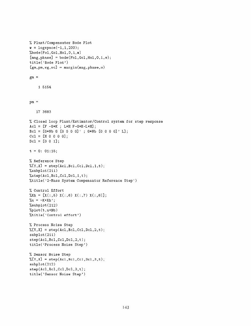
% Plant/Compensator Bode Plot
w = logspace(-1,1,200);
%bode(Fol,Gol,Hol,0,1,w)
[mag,phase] = bode(Fol,Gol,Hol,0,1,w);
title('Bode Plot')
[gm,pm,wg,wc] = margin(mag,phase,w)
gm =
1.5154
pm =
17.3683
% Closed loop Plant/Estimator/Control system for step response
Acl = [F -G*K ; L*H F-G*K-L*H];
Bcl = [G*Nb G [0 0 0 0]' ; G*Nb [0 0 0 0]' L];
Ccl = [H 0 0 0 0];
Dcl = [0 0 1];
t = 0:.01:15;
% Reference Step
%[Y,X] = step(Acl,Bcl,Ccl,Dcl,1,t);
%subplot(211)
%step(Acl,Bcl,Ccl,Dcl,1,t);
%title('2-Mass System Compensator Reference Step')
% Control Effort
%Xh = [X(:,5) X(:,6) X(:,7) X(:,8)];
%u = -K*Xh';
%subplot(212)
%plot(t,u+Nb)
%title('Control effort')
% Process Noise Step
%[Y,X] = step(Acl,Bcl,Ccl,Dcl,2,t);
subplot(211)
step(Acl,Bcl,Ccl,Dcl,2,t);
title('Process Noise Step')
% Sensor Noise Step
%[Y,X] = step(Acl,Bcl,Ccl,Dcl,3,t);
subplot(212)
step(Acl,Bcl,Ccl,Dcl,3,t);
title('Sensor Noise Step')
143

−3 −2 −1 0 1 2 3−3
−2
−1
0
1
2
3
Real Axis
Imag
Axi
s
SRL for LQE
−5 0 5−5
−4
−3
−2
−1
0
1
2
3
4
5
Real Axis
Imag
Axi
s
Plant/Compensator Root Locus
144
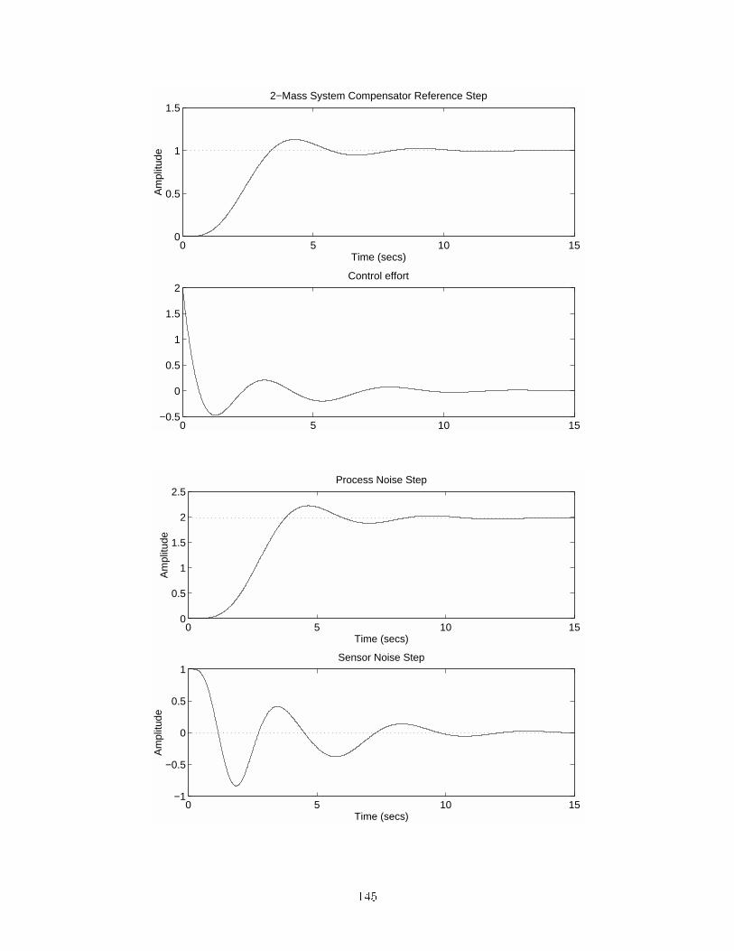
0 5 10 150
0.5
1
1.5
Time (secs)
Am
plitu
de
2−Mass System Compensator Reference Step
0 5 10 15−0.5
0
0.5
1
1.5
2Control effort
0 5 10 150
0.5
1
1.5
2
2.5
Time (secs)
Am
plitu
de
Process Noise Step
0 5 10 15−1
−0.5
0
0.5
1
Time (secs)
Am
plitu
de
Sensor Noise Step
145

4.2.3 Alternate reference input methods
_bx = F bx + Gu+ L(y Hbx)u = Kbx
With additional reference the equations are :
_bx = (F LH GK)bx+ Ly +Mr
u = kbx+Nr
Case 1 :
M = G N
N = N
This is same as adding normal reference input.
Case 2 :
N = 0
M = L
) _bx = (F GK LH)bx+ L(y r)
This is same as classical error feedback term.
Case 3:
M and N are used to place zeros.
Transfer function
) y
r=N (s)b(s)
e(s)c(s)
where
(s) = det(sI A+ MK)
M =M
N
N for unity gain.
Now estimator poles are not cancelled by zeros. The zeros are placed so as to get good tracking
performance.
146

4.3 Discrete Estimators
4.3.1 Predictive Estimator
xk+1 = xk + uk + 1w
y = Hx+ v
Estimator equation
) xk+1 = xk + uk + Lp(yk yk)
This is a predictive estimator as xk+1 is obtained based on measurement at k.
~xk+1 = xk+1 xk+1 = ( LpH)~xk + 1w Lpv
e(z) = det(zI + LpH)
Need O(,H) to build estimator.
4.3.2 Current estimator
Measurement update: bxk = xk + Lc(yk H xk)
Time update:
xk+1 = bxk + uk (128)
These are the equations for a discrete Kalman Filter (in steady state).
Γ Σ z1-
+
+
x_
H− +
y
L c
++
Φ Σ
Σ
x
u
Estimator block diagram
Substitute bx into measurement update equation:
) xk+1 = [xk + Lc(y H x)] + uk
= xk +Lc(y H xk) + u
147

Comparing with predictive estimator
Lp = Lc
~xk+1 = ( LcH)~xk
Now
O[; H]
should be full rank for this estimator.
Oc =
0BBBB@H
H2
...
Hn
1CCCCA = Op
detOc = detOpdet
) Cannot have poles at origin of open loop system.
Lc = 1Lp
4.4 Miscellaneous Topics
4.4.1 Reduced order estimator
If one of the states xi = y, the output, then there is no need to estimate that state.
Results in more complicated equations.
4.4.2 Integral control
Σ Σ+
+
+
−
r xi.
1−s
xi
-Ki
uF,G,H
-K
y
_x = Fx+ Gu
y = Hx
_xi = y + r = Hx+ r
148

)
_xi_x
!=
0 H0 F
! xix
!+
0
G
!u
u =Ki K
xix
!Gains can be calculated by place command.
Ki K
= place(
0 H0 F
!;
0
G
!; P )
n+1 poles can be placed.
Controllable if F;G are controllable and F;G;H has no zeros at s = 0.
4.4.3 Internal model principle
The output y(t) is made to track arbitrary reference r(t) (e.g. sinusoidal tracking for a spinning
disk-drive).
Augment state with r dynamics.
Ex 1 :
_x = Fx+ Gu
y = Hx
_r = 0! constant step
Or
r w20r = 0! Sinusoid
Dene
e = y ras new state which is driven to zero.
4.4.4 Polynomial methods
b(s)
a(s)F,G,H,J K Nb(s)
α c(s)
Direct transformation between input/output transfer function.
Often advantageous for adaptive control.
149

5 Kalman
(Lecture)
150

6 Appendix 1 - State-Space Control
Why a Space? The denition of a vector or linear space is learned in the rst weeks of a linear
algebra class and then conveniently forgotten. For your amusement (i.e. you-will-not-be-held-
responsible-for-this-on-any-homework-midterm-or-nal) I will refresh your memory.
A linear vector space is a set V, together with two operations:
+ , called addition, such that for any two vectors x,y in V the sum x+y is also a vector in V
, called scalar multiplication, such that for a scalar c 2 < and a vector x 2 V the product c Vis in V . 2
Also, the following axioms must hold:
(A1) x+ y = y + x; 8x; y 2 V (commutativity of addition)
(A2) x+ (y + z) = (x+ y) + z; 8x; y; z 2 V (associativity of addition)
(A3) There is an element in V, denoted by 0v (or 0 if clear from the context), such that
(x+ 0v = 0v + x = x); 8x 2 V (existence of additive identity)
(A4) For each x 2 V , there exists an element, denoted by x, such that
x+ (x) = 0v (existence of additive inverse)
(A5) For each r1; r2 in < and each x 2 V ,r1 (r2 x) = (r1r2) x
(A6) For each r in < and each x; y 2 V ,r (x+ y) = r x+ r y
(A7) For each r1; r2 in < and each x 2 V ,(r1 + r2) x = r1 x + r2 x
(A8) For each x 2 V ,1 x = x
Example 1: n-tuples of scalars. (We will not prove any of the examples.)
<n 4
=
8>>>>><>>>>>:
2666664x1x2:
:
xn
3777775 j xi 2 <9>>>>>=>>>>>;
Example 2: The set of all continuous functions on a nite interval
C[a; b] 4= ff : [a; b]! < j f is continuousg
2< is used to denote the eld of real numbers. A vector space may also be dened over an arbitrary eld.
151

A subspace of a vector space is a subset which is itself a vector space.
Example 1
N (A)4
=x 2 <q jAx = 0;A 2 <pq
is a subspace of <q called the nullspace or A.
Example 2
R(A)4
=x 2 <p j 9u 2 Rq Au = x;A 2 <pq
is a subspace of <p called the range of A.
And nally a very important example for this class.
Example 3
fx 2 Cn[<+] j _x = Ax for t 0g
is a subspace of Cn[<+] (continuous functions: <+ ! <n). This is the set of all possible trajectoriesthat a linear system can follow.
152

7 Appendix - Canonical Forms
Controller
Ac =
264 a1 a2 a31 0 0
0 1 0
375
Bc =
264 1
0
0
375Cc =
hb1 b2 b3
iAc is top companion
153

Observer
Ao =
264 a1 1 0
a2 0 1
a3 0 0
375
Bo =
264 b1b2b3
375Co =
h1 0 0
iAo is left companion
154

Controllability
Aco =
264 0 0 a31 0 a20 1 a1
375
Bco =
264 1
0
0
375Cco =
h1 2 3
iAco is right companion
155

Observability
Aob =
264 0 1 0
0 0 1
a3 a2 a1
375
Bob =
264 123
375Cob =
h1 0 0
iAob is bottom companion
G(s) =b1s
2 + b2s + b3
s3 + a1s2 + a2s+ a3=
1X1
isi
156

Part VII
Advanced Topics in Control
1 Calculus of Variations - Optimal Control
1.1 Basic Optimization
1.1.1 Optimization without constraints
minuL(u) without constraints.
Necessary condition@L
@u= 0
@2L
@u2 0
1.1.2 Optimization with equality constraints
minu
L(x; u) subject to f(x; u) = 0
Dene
H = L(x; u) + Tf(x; u)| z \adjoin" constraints
Since u determines x
H = L
Dierential changes on H due to x and u
dH =@H
@xdx+
@H
@udu
We want this to be 0, so start by selecting such that
@H
@x= 0
@H
@x=@L
@x+ T
@f
@x= 0 (129)
) T = @L@x
@f
@x
1
) dL = dH =@H
@udu
157

For a minimum we need
dL
du= 0
)
@H
@u= 0 =
@L
@u+ T
@f
@u= 0 (130)
Summary
minu
L(x; u) such that f(x; u) = 0
@H
@x= 0;
@H
@u= 0
where
H = L(x; u) + Tf(x; u)
Example
minuL(u) =
1
2
x2
a2+u2
b2
!such that
f(x; u) = x+mu c = 0
H =1
2
x2
a2+u2
b2
!+ (x+mu c)
@H
@x=
x
a2+ = 0
@H
@u=u
b2+ m = 0
x+mu c = 0
There are 3 equations and three unknowns x,u,
) x =a2c
a2 +m2b2; u =
b2mc
a2 +m2b2; =
c
a2 +m2b2
158

1.1.3 Numerical Optimization
Non-linear case
minuL(x; u) + Tf(x; u) = min
uH
wheref(x; u) = 0
Setting @H
@x= 0 and @H
@u= 0 leads to an algorithm for computing u:
1. Guess u, for f(x; u) = 0 solve for x.
2. T = @L
@x
@f
@x
1:
3. @H
@u= @L
@u+ T @f
@u; test for @H
@u= 0.
4. u u @H@u
Therefore one does a gradient search.
Related optimization
Inequality constraints L(x; u) subject to f(x; u) 0, requires Kuhn-Tucker conditions.
If L and f linear in x; u then use Linear Programming.
Constrained optimization + calculus of variations ! Euler-Lagrange Equations.
1.2 Euler-Lagrange and Optimal control
1.2.1 Optimization over time
Constraint
_x = f(x; u; t); x(t0)
with cost
minu(t)
J = '(x(tf); tf) +
Ztf
t0
L(x((t); u(t); t) dt
Adjoin the constraints
J = '(x(tf); tf) +
Ztf
t0
L(x(t); u(t); t) + t(t) ff(x; u; t) _xg dt
where the Hamiltonian is dened as
H = L(x(t); u(t); t) + T (t)f(x; u; t):
Using integration by parts on the T _x term
J = '(x(tf); tf) T (tf )x(tf) + T (t0)x(t0) +
Ztf
t0
H + _Tx dt:
159

To minimize variation in J due to variations in the control vector u(t) for xed times t0 and tfminimize
J =
@'
@x T
xjt=tf +
hTx
ijt=t0 +
Ztf
t0
@H(x; u; t)
@x+ _T
x+
@H(x; u; t)
@uu
dt
Choose (t) such that the x coecients vanish
_T = @H@x
= @L@x T @f
@x(131)
T (tf) =@'
@x(tf): (132)
Then
J = T (t0)x(t0) +
Ztf
t0
@H
@uu dt
But we still want to minimize J for variations u at the optimal u yielding the optimal J (i.e., we
need @ J@u
= 0). Then@H
@u= 0 =
@L
@u+ T
@f
@u(133)
is called an `in uence function' on J .
Equations 131, 132 and 133 dene the Euler Lagrange Equations for a two-point boundary problem.
Solution of these equations leads to Pontryagin's minimum principle (w/o proof)
H(x; u; ; t) H(x; u; ; t)
Summary: given the cost
minu(t)
J = '(x(tf ); tf) +
Ztf
t0
L(x((t); u(t); t)dt;
and constraint
_x = f(x; u; t);
_ = @f
@x
T
@L
@x
T= @H
@x
T
where u is determined by@H
@u= 0 or
@f
@u
T+
@L
@u
T= 0:
x(t0)
is given;
(tf) =
@'
@x
Ttf
is the boundary condition. In general this leads to some optimal solution for u(t), which is deter-
mined by initial value x(t0) and nal constraint '(x(tf); tf), resulting in open-loop control since
the control is xed without feedback.
160

1.2.2 Miscellaneous items
The family of optimal paths for all initial conditions x(t0), 0 < t0 < tf is called a `eld of
extremals'.
If we solve for all states such that u = function(x; t) then this is the `optimal feedback control
law'.
J = J(x; t) gives the optimal return function.
1.3 Linear system / ARE
Consider the time-varying linear system
_x = F (t)x +G(t)u; x(tf )! 0
with cost function
J =1
2(xTSfx)t=tf +
1
2
Ztf
t0
xTQx+ uTRudt
with Q and R positive denite.
Then using the Euler-Lagrange equations from Equation 133
@H
@u= 0 = Ru+GT
so that the control law is
u = R1GT
and from Equation 131_ = Qx FT
with boundary condition
(tf) = Sfx(tf )
from Equation 132. Assimilating into a linear dierential equation"_x_
#=
"F GR1GT
Q FT
# "x
#;
x(t0)
(tf ) = Sfx(tf )
Try a solution that will convert the two-point boundary problem to a one-point problem. As a
possible solution try (t) = S(t)x(t)
_Sx+ S _x = Qx FTSx
so that
( _S + SF + FTS SGR1GTS + Q)x = 0
resulting in the matrix Ricatti equation
_S = SF FTS + SGR1GTS Q; with S(tf) = Sf
Note that
u = R1GTS(t)x(t) = K(t)x(t)
161

where K(t) is a time-varying feedback.
_S = 0 gives the steady state solution of the Algebraic Ricatti Equation (A.R.E) where tf ! 1.
Then K(t) = K ie state feedback.
The A.R.E may be solved
1. by integrating the dierential Ricatti equation to a xed point
2. symbolically
3. by eigen value decomposition
4. with the schur method
5. with a generalized eigen formulation.
6. MATLAB
1.3.1 Another Example
_x = ax+ u
J =
Z1
0u2 + 2x2
with open loop pole at s = a. Steady state A.R.E gives
sF + FT s sGR1GT s+ Q = 0
as+ as s:1:1:1:s+ 2 = 0
Therefore
s2 2as 2 = 0
and
s =2a
p4a2 + 42
2= a
qa2 + 2
K = R1GTs = s = a+qa2 + 2
with the closed loop poles at s = a k. See gure 17.
1.4 Symmetric root locus
Take the Laplace transform of the Euler Lagrange equations for the linear time invariant case of
example 1.3.
sx(s) = Fx(s) + Gu(s)
s(s) = Qx(s) FT(s)
u(s) = R1GT(s)
Q = HTH2 and R = 1:
162

-a a
u=-kx
ρ=0ρ= large
Figure 17: Closed loop poles
Then
u(s) = GT (sI + FT )1HTH2(sI F )1Gu(s)where
GT (s) = GT (sI + FT )1HT
and
G(s) = H(sI F )1G;the open loop transfer function. Thenh
1 + 2GT (s)G(s)iu(s) = 0
giving the symmetric root locus (SRL).
Has 2N roots for the coupled system of x; of order N .
as t! 1 u(t) = K1x(t) it becomes an Nth order system with N stable poles.
1.4.1 Discrete case
Given the discrete plant
x(k + 1) = x(k) + u(k);
u = Kxthe task is to minimize the cost function
J =1
2
NXk=0
hxT (k)Qx(k) + uT (k)Ru(k)
i:
Using a Lagrange multiplier
J =1
2
NXk=0
hxT (k)Qx(k) + uT (k)Ru(k) + T (k + 1)(x(k+ 1) + x(k) + u(k))
ileads to the Euler Lagrange equations
@H
@u(k)= uT (k)R+ T (k+ 1) = 0 (134)
@H
@(k+ 1)= x(k + 1) + x(k) + u(k) = 0 (135)
@H
@x(k)= T (k + 1)+ xT (k)Q T (k) = 0 (136)
(137)
163

From the cost function clearly u(N) = 0 and from Equation 134 (N + 1) = 0 so that from
Equation 136
(N) = Qx(N):
Again choosing
(k) = S(k)x(k)
it follows that
u(k) = R1T(k+ 1)
with the Discrete Ricatti Equation (non-linear in S)
S(k) = T
hS(k + 1) S(k + 1)N1TS(k + 1)
i+Q;
with the end condition
S(N) = Q
and where
N = R+ TS(k+ 1):
The feedback gain then is
K(k) =hR+ TS(k + 1)
i1
TS(k+ 1):
Note that the minimum cost is
J =1
2xT (0)S(0)x(0):
1.4.2 Predictive control
Here the cost is taken as
J(x; ut!t+N) =t+N1Xk=t
L(K; x; u)
giving u(t); : : :u(t +N). Only u(t) = K(t)x(t) is used, and the RHC problem re-solved for time
t + 1 to get u(t + 1). u(t) provides a stable control if N the order of the plant, and the plant is
reachable and observable.
Guaranteed stabilizing if prediction horizon length exceeds order of plant.
(SIORHC) = stabilizing input-output receding horizon control.
This is popular for slow linear and non-linear systems such as chemical batch processes.
See `Optimal predictive and adaptive control' Mosca.
164

1.4.3 Other applied problems
Terminal constraint of x
Here x(tf ) = xf or
(x(tf )) = 0:
Adjoin vT(x(tf )) to J . Then
T (tf ) =
@'
@x+ vT
@
@x
t=tf
:
Examples include 1) robotics for a xed endpoint at xed time, 2) transfer of orbit radius in given
time.
Thrust
r(0), t(0)
t(F), r(F)
Unspecied time
Want to move an arm from A to B, but do not know how long it will take. A 4'th condition is
required together with the prior Euler Lagrange equations to minimize time as well@'
@t+ Tf + L
t=tf
= 0:
Some minimum time problems.
Missile trajectory.
_x = f(x; u; t) = f(t)x+ g(t)u
J(u) =
Ztf
t0
1 dt = tf t0 ) L = 1
such that ju(t)j 1 is a nite control. Solving,
H = L+ T [f(t) + g(t)u] ; L = 1
165

Clearly to minimize H the resulting optimal u is `bang-bang control'
u =
(1 Tg < 0
1 Tg > 0
)
To solve for
@H@x
= _T = @L@x T @f
@x
so that is obtained as the solution to
_T = T f(t)
and
T [fx+ gu] = 1:
Double integrator. Consider the system
_x1 = x2
_x2 = ax2 + u
x 2
x 1
u=-1
u=+1
x(0)
µ
µ
=-1
=+1
Start
path
Figure 18: Double integrator
Other minimum-time problems.
robotics (2 and 3 link arms)
min-time orbits
brachistochron problem (solutions are cycloids).
minimum control (ex. fuel) problems st 1 ui 1 ) bang-o-bang control.
166

shifting bead
B
A
A -> B in minimum time:
shape of string?
θ
Figure 19: Brachistochron problem
2 Dynamic Programming (DP) - Optimal Control
2.1 Bellman
Dynamic Programming represents an alternative approach for optimization.
ca
b
J Jab bc
Suppose that we need to determine an optimal cost to go from point a to point c.
If the optimal path from a to c includes the path from a to b, then the path from b to c is
the optimal path from b to c.
i.e., Jac= Jab + J
bc
Bellman: An optimal policy has the property that whatever the initial state and the initial
decision are, the remaining decisions must constitute an optimal policy with regard to the
state resulting from the rst decision.
167

2.2 Examples:
2.2.1 Routing
bf
c
d
e
J
J
J
J
bd
cf
df
efJ be
J bc
*
*
*
Start out with paths bc or bd or be.
The optimal path from b to f is hence the minimum of Jbc + Jcf, Jbd + J
df, Jbe + J
ef
Jcf, J
dfand J
efare determined by back-tracking.
The viterbi algorithm for processing of speech is based on dynamic programming.
2.2.2 City Walk
Final Pointa d e h
b c f g
5 5 2 2
8 3
3
8
39
N
EW
S
Want to 'walk' from c to h. Which is the optimal path?
We have two choices; proceed along path from either c to d or c to f .
So, Ccdh
= Jcd + Jdh
= 15
Ccfh
= Jcf + Jfh
= 8
Jch
= minfCcdh; C
cfhg
= minf15; 8g= 8
As with the routing example, we need to know Jdh
and Jfh
initially, which implies a back-
tracking problem.
2.3 General Formulation
JkN
(x(k)) = minU(k)
[Jk;k+1(X(k); U(k))+ Jk+1;N (X(k+ 1))]
168

) We are minimizing only with respect to U(k), instead of U's over the entire path. Let
k! N k. So,
JNk;N (X(Nk)) = min
U(Nk)[JNk;Nk+1(X(Nk); U(N k))+J
N(k1);N(X(Nk+1))]
) JN(k1) ! JNk;N
This implies a backward recurrence.
Start at the last time step and dene JNN
4
= JNN .
Then solve for JN1;N and work backwards.
Curse of Dimensionality: For all possible X , suppose that X 2 <3 and Xi can take-on
100 values. Thus we need to have already found and stored 102 102 102 = 106 values for
JN(k1);N
to solve for JNk;N
.
Dynamic programming is not practical unless we can intelligently restrict the search space.
2.4 LQ Cost
Given
Xn+1 = AXn + bUn
Yn = HXn
we have the following:
J0;N =1
2
N1Xk=0
(XT (k)QX(k) + UT (k)RU(k)) +1
2XT(N)QX(N)
Need to minimize J0;N over time. We saw before that the solution to the above involves a Ricatti
equation. By denition,
J0;N (X0) = minU0;U1;U2;:::;UN
J0;N(X0)
Let's write this as follows:
J0;N =1
2XT (0)Q(0)X(0)+ UT (0)RU(0)| z
cost at k = 0 due to U0
+1
2
N1Xk=1
(XT(k)QX(k) + UT (k)RU(k))| z cost to go from k = 1
+XT (N)QX(N)
= minU2<
f XT
0 QX0 + UTRU| z initial cost to go from X0 to AX0+bU
+ J1;N(AX0 + bU)| z min. cost starting at AX0+bU0
g
Next, express the cost at the nal state as the following.
JNN
=1
2XT (N)QX(N)
Let S(N)=Q,
JN1;N =1
2XT (N 1)QX(N 1) +
1
2UT (N 1)RU(N 1) +
1
2XT(N)S(N)X(N) (138)
169

where, X(N) = (AX(N 1) +BU(N 1))
JN1;N
4
= minu(N1)
JN1;N
Take@JN1;N
@U(N 1)= 0 = RU(N 1) +BTS(N)[AX(N 1) +BU(N 1)]
(Exercise: Show that @2J
@U2 is P.D.)
) U(N 1) = [R+BTS(N)B]1S(N)A| z K(N1)
X(N 1)
Substitute U(N 1) back in equation 138. ) JN1;N = 1
2XT(N 1)S(N 1)X(N 1)
where S(N 1) is the same as we derived using the Euler-Lagrange approach.
S(N 1) is given by a Ricatti Equation.
Continue by induction.
Comments
J is always quadratic in X . This makes it easy to solve.
As N !1, this becomes the LQR. S(k) = S, and Jk= XT
kSXk
2.5 Hamilton-Jacobi-Bellman (HJB) Equations
This is the generalization of DP to continuous systems.
J = '(X(tf); tf) +
Ztf
t
L(X(); U(); )d
such that, F (X;U; t) = _X. Need to minimize J using DP.
J(X(t); t) = minU();t<<t+4t
[
Zt+4t
t
Ld + J(X(t+4t); t+4t)]
by the principle of optimality.
Expand J(X(t+4t; t+4t)) using Taylors series about (X(t); t). So,
J(X(t); t) = minu();t<t+4t
[
Zt+4t
t
L(X;U; )d + J(X(t); t) + [@J
@t(X(t); t)]4t
+[@J
@X(X(t); t)]T [ (X(t+4t)| z
F (X;U;t)4t+ higher order terms
X(t)]]
= minU(t)
[L(X;U; t)4t+ J(X(t); t) +@J
@t(X(t); t)4t| z
does not depend on U
+@J
@X(X(t); t)[F (X;U; t)]4t]
170

Divide by 4t and take limit as 4t! 0
0 =@J
@t(X(t); t) = min
u[L(X;U; t) +
@J
@X(X(t); t)F (X;U; t)]
Boundary Condition: J(X(tf ; tf) = '(X(tf ; tf)
Dene Hamiltonian as:
H(X;U;@J
@X; t)
4
= L(X;U; t) +@J
@X(X(t); t)[F (X;U; t)]
(recall H from Euler-Lagrange equation ) T (t) = @J
@X(X(t); t) in uence function)
The optimal Hamiltonian is given by:
H(X;U;@J
@X; t) = min
U(t)H(X(t); U(t);
@J
@X; t) (139)
Thus, 0 =@J
@t+H(X;U;
@J
@X; t) (140)
Equations 139 and 140 are the HJB equations.
Exercise: Derive the E-L equations from the H-J-B Equation.
2.5.1 Example: LQR
_X = A(t)X + B(t)U
J =1
2XT (tf)SfX(tf) +
1
2
Ztf
t0
XTQX + UTRUdt
H =1
2XTQX +
1
2UTRU +
@J
@X[AX +BU ]
So, to minimize H,
@H
@U= RU + BT
@J
@X= 0
(note that @2H
@U2 = R is P.D. ! global min.)
) U = R1BT@J
@X
Thus,
H =1
2XTQX +
1
2
@J
@X
T
BR1BT@J
@X+@J
@X
T
AX @J
@X
T
BR1BT@J
@X
=1
2XTQX 1
2
@J
@X
T
BR1BT@J
@X+@J
@XAX
Thus, the H-J-B equation is:
0 =@J
@t+1
2XTQX 1
2
@J
@XBR1BT
@J
@X+@J
@X
T
AX
171

With boundary conditions,
@J
@X(X(tf); tf) =
1
2XT (tf )SfX(tf)
Let's guess J =1
2XTS(t)X(t)| z
quadraticThen we get,
0 =1
2XT _SX +
1
2XTQX 1
2XTSBR1BTSX +XTSAX
let SA =1
2[SA+ (SA)T ]| z symmetric
+1
2[SA (SA)T ]| z un-symmetric
Also, XT (1
2[SA (SA)T ])X = 0
Thus,
0 =1
2XT _SX +
1
2XTQX 1
2XTSBR1BSX +
1
2XTSAX +
1
2XTATSX
Now, this must hold for all X
) 0 = _S + Q SBR1BS + SA+ ATS
which is the Ricatti equation we saw before. With boundary conditions,
S(tf) = Sf
2.5.2 Comments
Equation 140 is another form of Pontryagin's minimal principle.
Involves solving partial dierential equations which may not lead to closed form solution.
For global optimality, we need:
@2H
@U2 0) Legendre-Clehsch condition
J is a necessary condition to satisfy the H-J-B equations. It can also be proved that J is a
sucient condition.
Solution often requires numerical techniques or the method of characteristics.
The H-J-B equations relate dynamic programming to variational methods.
172

3 Introduction to Stability Theory
3.1 Comments on Non-Linear Control
3.1.1 Design Methods
Linearization of the plant followed by techniques like adaptive control.
Lots of "rules of thumb", which are not well-dened.
Not as easy as Bode, root-locus (i.e., classical linear control).
Methods include: DP, E-L, neural and fuzzy.
3.1.2 Analysis Methods
Many analysis methods for non-linear systems.
Equivalent concepts of controllability and observability for non-linear systems, but very hard
to prove.
Some common ones in control: describing functions, circle theorems, Lyapunov methods,
small-gain theorem, passivity (the latter two are very advanced methods).
Most of the analysis methods are concerned with stability issues of a given system _X =
F (X;U).
3.2 Describing Functions
This is an old method which is not always rigorous.
Consider systems of the following conguration.
NL G(Z)
where, NL stands for simple non-linearities like any of the following:
173

Consider the following.
NLInput Output
Let input=A sin !t. Then, output=A0 +P1
n=1 Yn sin(n!t+ n) (sum of harmonics).
Describing function D(A) =Y1
A6 1
=fundamental of output
input
Example: Consider X to be a saturation function of the following form:
X4=
8><>:+m X > 1
kX jX j < 1
m X < 1
9>=>;
xk
-m
m
So,
D(A) =
(2karcsin m
Ak+ 2m
A
q1 m
Ak
2 Ak
m> 1
k Ak
m 1
)
174

m
Ak
D(A)
k
Note:
For certain regions below saturation, there is no distortion.
As the gain is increased, Y1 decreases.
Describing functions give us information regarding stability and limit cycles.
Steps:
1. Plot the Nyquist of G(Z).
2. Plot 1D(A)
on the same graph.
Re
Im
gives amplitude and frequencyof possible limit cycle
-1/D(A)
G(w)
If the 2 plots intersect, then there may exist instabilities.
3.3 Equivalent gains and the Circle Theorem
This is a rigorous way of formalizing the describing functions D(A) (developed in the '60s).
175

Consider the following non-linearity:
x
φ (x)slope k2
slope k1
The N-L is bounded with two lines of slope k1 and k2, such that:
k1 (X)
X k2
Hence,
(X) 2 sector[k1; k2]
Example: quantizer
x
Azermans Conjecture, 1949Consider the following system:
176
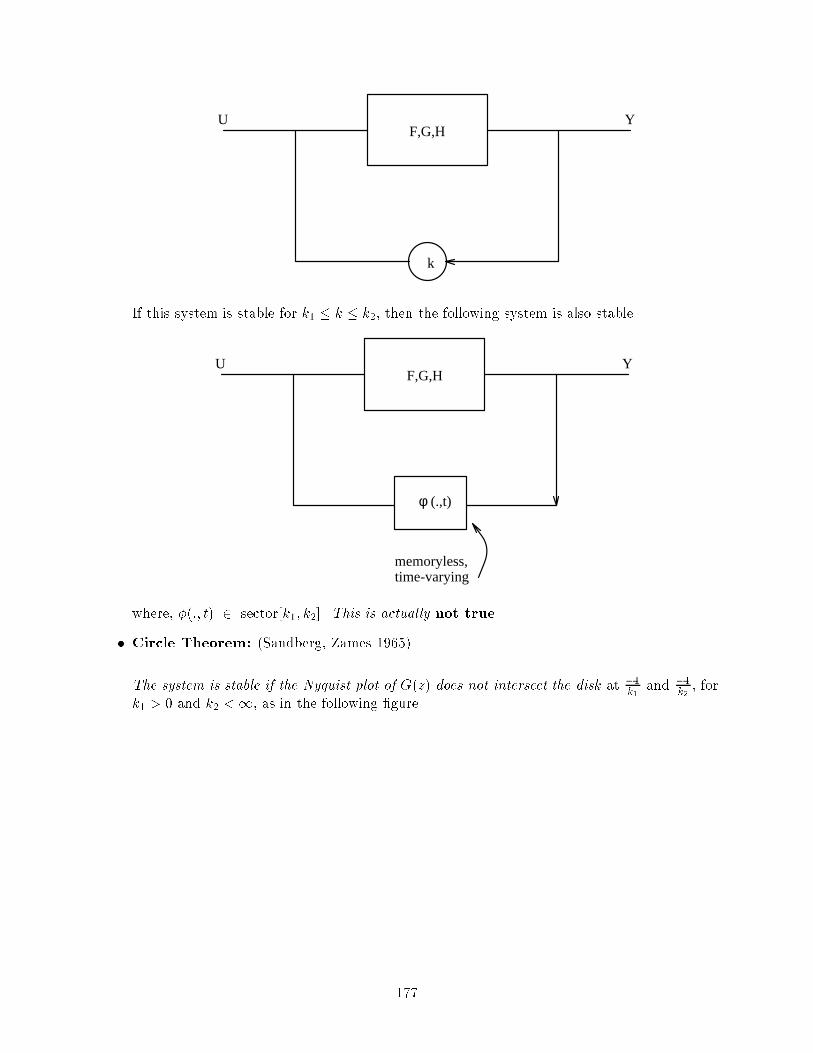
F,G,H
k
YU
If this system is stable for k1 k k2, then the following system is also stable.
F,G,HYU
(.,t)φ
memoryless,time-varying
where, (:; t) 2 sector[k1; k2]. This is actually not true.
Circle Theorem: (Sandberg, Zames 1965)
The system is stable if the Nyquist plot of G(z) does not intersect the disk at 1k1
and 1k2, for
k1 > 0 and k2 <1, as in the following gure.
177

-1
k2
Nyquist
-1
k1
disk
Now, if k1 = 0) 1k1
=1, then the following case would result.
-1
k2
make sure the quantizers Nyquistdoes not cross this boundary
A related theorem is Popovs theorem, for time-independent (t).
3.4 Lyapunovs Direct Method
If _X = F (X; t)
where, F (0; t) = 0, then, is X = 0 stable at 0?
We proceed to dene stability in a Lyapunov sense.
178
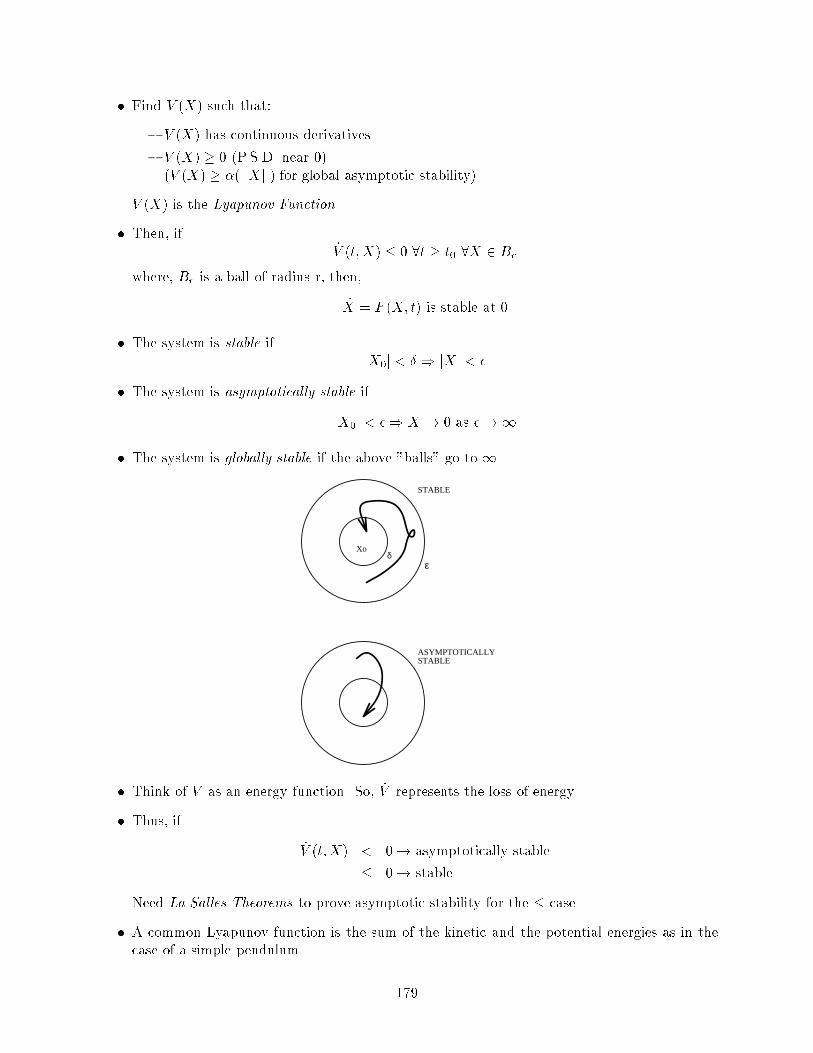
Find V (X) such that:
V (X) has continuous derivatives.
V (X) 0 (P.S.D. near 0)
(V (X) (jjX jj) for global asymptotic stability).
V (X) is the Lyapunov Function.
Then, if_V (t; X) 0 8t t0 8X 2 Br
where, Br is a ball of radius r, then,
_X = F (X; t) is stable at 0
The system is stable if
jX0j < ) jX j <
The system is asymptotically stable if
jX0j < ) X ! 0 as !1
The system is globally stable if the above "balls" go to 1.
ASYMPTOTICALLYSTABLE
STABLE
Xoδ
ε
Think of V as an energy function. So, _V represents the loss of energy.
Thus, if
_V (t; X) < 0! asymptotically stable
0! stable
Need La Salles Theorems to prove asymptotic stability for the case.
A common Lyapunov function is the sum of the kinetic and the potential energies as in the
case of a simple pendulum.
179

3.4.1 Example
Let_X = sinX
Here, X = 0 is an equilibrium point. So, let
V (X) = X2
) _V = 2X _X = 2X sinX
Note that the above V (X) is not a valid Lyapunov function for unlimited X . So, we need to nd
a "ball" such that it is a Lyapunov function. But, sinX 12X for 0 < X < C (C is a constant)
sin x 0.5x
xπ
−π
Thus,_V X2 for jX j C
So,_V 0 within the "ball"
) 0 is an asymptotically stable equilibrium point.
t
x(t)
unstable
asymptotically stable
0
near 0, x(t) 0 as t 0
180

3.4.2 Lyapunovs Direct Method for a Linear System
Let_X = AX
Therefore, postulate
V (X) = XTPX
where, P = PT 0
J(X0) =
Z1
0XTQXdt
= XT
0
Z1
0eA
TtQeAtdt| z P
X0
= V (X0)
) _V = XTQX < 0
where, Q = ATP + PA) Lyapunov Equation
If A is asymptotically stable, then for Q = QT 0, there is a unique P = PT 0, such that,
ATP + PA +Q = 0
Exercise: Plug-in u = kX and show we get the algebraic Ricatti equation.
This approach is much harder for time-varying systems.
3.4.3 Comments
Lyapunovs theorem(s) provide lots of variations as far as some of the following parameters
are concerned.
Stability
Global stability
Asymptotic global stability, etc.
What about adaptive systems? An adaptive system can be written as a non-linear system
of higher order.
YUW
So,
Wk+1 = Wk + F (U; Y; C)
) use Lyapunov function to determine stability.
Y = WU or Y = F (X;U;W )
181
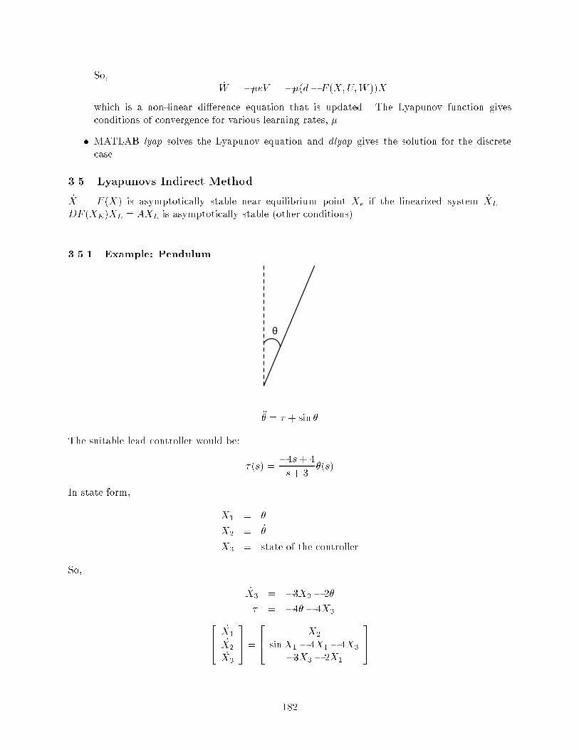
So,_W = eV = (d F (X;U;W ))X
which is a non-linear dierence equation that is updated. The Lyapunov function gives
conditions of convergence for various learning rates, .
MATLAB lyap solves the Lyapunov equation and dlyap gives the solution for the discrete
case.
3.5 Lyapunovs Indirect Method
_X = F (X) is asymptotically stable near equilibrium point Xe if the linearized system _XL =
DF (XE)XL = AXL is asymptotically stable (other conditions).
3.5.1 Example: Pendulum
θ
= + sin
The suitable lead controller would be:
(s) =4s+ 4
s+ 3(s)
In state form,
X1 =
X2 = _
X3 = state of the controller
So,
_X3 = 3X3 2
= 4 4X3264 _X1
_X2
_X3
375 =264 X2
sinX1 4X1 4X3
3X3 2X1
375
182

Linearize this at X=0.
) A =
264 0 1 0
3 0 42 0 3
375So,
eig A = -1, -1, -1) stable
Hence, we have designed a lead-lag circuit which will give asymptotic stability for some region
around zero. The non-linear structure is stable as long as we start near enough 0.
3.6 Other concepts worth mentioning
Small gain theorem.
H 1
H 2 +
+
U
Y1e1
e2
2Y2
1U
A system with inputs U1 and U2 and outputs Y1 and Y2 is BIBO stable, provided H1 and H2
are BIBO stable and the product of the gains of H1 and H2 is less than unity. This is often
useful for proving stability in adaptive control.
Passivity.
These are more advanced and abstract topics used for proving other stability theorems. They are
also useful in adaptive systems.
4 Stable Adaptive Control
4.1 Direct Versus Indirect Control
Direct control
Adjust control parameters directly.
Model reference adaptive control is a direct control method.
Indirect control
Plant parameters are estimated on-line and control parameters are adjusted.
183

Gain scheduling is an open loop indirect control method where predetermined control is
switched based on current plant location.
Gain Scheduling
4.2 Self-Tuning Regulators
Self-Tuning Regulator
A Control Structure
184

System identication is carried out by RLS, LMS etc.
Issues: The inputs should persistently excite the plant so that system identication is properly
done.
Control Design
Time varying parameters
PID
LQR
Kalman (If the system is linearized at each time point then it is called Extended Kalman)
Pole-placement
Predictive control
The design is often done directly in polynomial form rather than state space. This is
because system ID (e.g. using RLS) provides transfer functions directly.
Issues:
Stability
Robustness
Nonlinear issues
4.3 Model Reference Adaptive Control (MRAC)
+
++
M
P
Km
s+am
Co
do
s+ap
Kpu
r
e
ym
yp
Model Reference Adaptive Control - An example
_yp(t) = ap yp(t) +Kpu(t) (141)
_ym(t) = am ym(t) +Kmr(t)
185

Let
u(t) = co(t)r(t) + do(t)yp(t)
Substitute this u(t).
Note that if
co=Km
Kp
do=ap amKp
Then
_yp(t) = am yp(t) +Kmr(t)
Consider Gradient descent
@
@t= @e
2o()
@= 2eo
@eo()
@
= 2eo@yp
@
++
P
Co
do
s+ap
Kpur yp
yp =
Kp
s + ap
!(doyp + rco)
@yp
@co= P r
@yp
@do= P yp
where
P =
Kp
s ap
!
If we don't know plant.
Just use proper sign of Kp and ignore P i.e. set P = 1 or
Use current estimates of Kp and ap (MIT Rule)
With P = 1
) _c = e r
_d = e yp
186

Is the system stable with this adaptation?
Dene
r = co co
y = do do
Then eo = yp ym
After some algebraic manipulations
_eo = am eo +Kp(r r + y eo + y ym)
_r = eo r_y = eo yp = e2
o eo ym
Dene Lyapunov function
V (eo; r; y) =e2o
2+Kp
2(2
r+ 2
y)
_V = ame2o +Kpreor+Kpye2o+Kpoeoym Kpreor Krye
2oKpyeoym
= am e2o<= 0
) This is a stable system since V is decreasing monotonically and bounded below.
lim V (t) as t!1 exist. Thus eo ! 0 as t! 1.
Indirect method can also be used
Estimate cKp; bap and design co and do.
4.3.1 A General MRAC
Plant bp(s) = Kp
bnp(s)bdp(s) = yp(s)
u(s)
Model
M(s) = Km
nm(s)
dm(s)=bym(s)br(s)
187

Model Reference Adaptive Control
Controller Structure
A Control Structure
Existence of solution
Adaptation Rules
Many variations
"Heuristic" Gradient descent
Try to prove stability and convergence
Start with Lyapunov function
Find adaptation rule.
Issues
Relative order of systems
Partial knowledge of some parameters.
188

5 Robust Control
Suppose plant P belongs to some family P ; Robust Control provides stability for every plant
in P . (Worst case design)
Nominal performance specications
y(s) =g(s)k(s)
1 + g(s)k(s)r(s) +
1
1 + g(s)k(s)d(s) g(s)k(s)
1 + g(s)k(s)n(s)
L = gk = open loop gain
J = 1 + gk = return dierence
S =1
1 + gk= sensitivity transfer function
T =gk
1 + gk= complementary transfer function
S + T = 1
(142)
Command tracking
Want gk large
S has to be small (low frequency)
Disturbance rejection
S has to be small (low frequency)
Noise suppression
T has to be small (high frequency)
189

Desired Open Loop Response
5.1 MIMO systems
A = GK(I +GK)1
where A is Transfer -Function Matrix
190

i(A) = (i(AA))
12 ! Singular values
S = (I + GK)1 T = GK(I + GK)1
Singular plots
Plots of i(A) Vs frequency, which are generalization of Bode plots.
5.2 Robust Stability
Suppose we design for G(s)
The design is robust if the closed loop system remains stable for true plant ~G(s)
5.2.1 Small gain theorem (linear version)
jG(s)K(s)j < 1) stability
jG(s)K(s)j jG(s)jjK(s)j
) Stability guaranteed if jG(s)jjK(s)j < 1
G(s)K(s)
-1
Instability according to Nyquist
191

5.2.2 Modeling Uncertainty
We use G(s) for design whereas the actual plant will be ~G(s).
~G(s) = G(s) + a(s)! Additive
~G(s) = (1 + m(s))G(s)! Multiplicative
192

5.2.3 Multiplicative Error
M(s) =G(s)K(s)
1 +G(s)(K(s)
Closed system is stable if
jmj <1
jGK(1 +GK)1j
) jmj <1
jT j
Bound the uncertainty
Suppose jmj <
This is stable if
jT j < 1
Smallest destabilizing uncertainty
(Multiplicative Stability Margin)
193

MSM =1
Mr
Mr = supw
jT (jw)j = jjT jj1 ! innity norm
This represents distance to -1 point on Nyquist plot.
For MIMO = sup
w
(T (jw)) = jjT jj1
For additive uncertainty
jaj <1
jKSjAdditive Stability Margin is given by
ASM =1
jjKSjj1
recall jT + Sj = 1
If we want MSM large then T has to be small. This is good for noise suppression but con icts
with tracking and disturbance.
Trade o
jjT jj1 < 1
jjKSjj1 1
T + S = 1
194
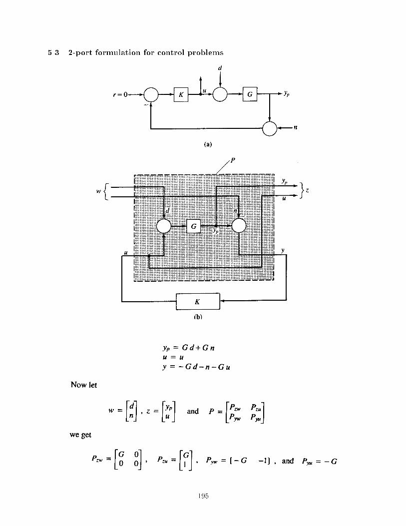
5.3 2-port formulation for control problems
195

closed loop transfer function from w to z is:
5.4 H1 control
Standard problem:
Find K(s) stabilizing so that jjTzwjj1
Optimal control
Find K(s) stabilizing to minimize jjTzwjj1Typically solve standard problem for , then reduce until no solution possible to get the
optimal control.
(LQG results from minjjTzw jj2)
Many assumptions like stabilizable, detectable for solution to exist.
Two port block diagram
Transfer function:
State-space:
Packed-matrix notation
196

H1 Controller
Controller
Estimator
Packed-Matrix Form
Controller/Estimator gains
H1 constants:
197

Closed loop system:
Necessary conditions for the above solutions are existence of Ricatti equations, and,
H1 Controller
198

5.5 Other Terminology
Generalization to nite horizon problems
jjTzwjj1 ! jjTzwjj[O;T ]
where [O,T] is induced norm i.e. L2[O; T ]
This is a much harder problem to solve as it is a 2-point boundary value problem
Loop Shaping: Design for characteristics of S and T.
Adjust open loop gains for desired characteristics (possibly by some pre-compensators)
Determine opt using H1 design and repeat if necessary.
May iterate (for example to reduce model order).
199

Part VIII
Neural Control
Neural control often provides an eective solution to hard control problems. This does not imply
that more traditional methods are necessarily incapable of providing as good or even better solu-
tions. The popularity of neural control can in part be attributed to the reaction by practitioners
to the perceived excessive mathematical intensity and formalism of recent development in modern
control theory. Although neural control techniques have been inappropriately used in the past, the
eld of neural control is now reaching a level of maturity where it is becoming more widely accepted
in the controls community.
Certain aspects of neural control are especially attractive, e.g., the ability to systematically deal with
non-linear systems, and simple generalizations to multi-input-multi-output problems. However, we
must caution students that this eld is still at its infancy. Little progress has been made to
understand such issues as as controllability, observability, stability, and robustness.
1 Heuristic Neural Control
We start with some \heuristic" methods of control which utilize neural networks in conjunction
with classical controllers. 1) Control by emulation, in which we simply attempt to learn an existing
controller. 2) Inverse and open-loop control. 3) Feedback control, where the feedback is ignored
during designing the controller. These methods, while rather ad-hoc, can be quite eective and are
common in industrial applications today.
1.1 Expert emulator
If a controller exists we can try to emulate it as illustrated below
r,x
controller
G
e
y
y
+
There is no feedback and we train with standard BP. This is useful if the controller is a human and
we want to automate the process.
An example of a network trained in this manner is ALVINN at CMU. The input to the controller
was a 30 by 32 video input retina and the output was the steering direction. The neural controller
was trained by \watching" a human drive. Fifteen shifted images per actual input were used
during training to avoid learning to just drive straight. Two hundred road scenes from the past
200

are stored and trained on to avoid \forgetting". Fifteen of the two hundred are replaced for each
new input image. Two networks were trained, one for single lane roads, and another for double
lane roads. Each network was also trained as an auto associator. The network with the best L.S.
reconstruction of the input image gave a condence level to determine which network got to drive
(*SHOW VIDEO).
1.2 Open loop / inverse control
Early systems were designed open loop making the neural controller approximately the inverse
of the plant: C P1.
Not all systems have inverses, such as the robotic arm illustrated below. (To resolve this problem,
it is necessary to incorporate trajectory constraints.)
Direct inverse modeling: as illustrated in the gure below, one could reverse the order of plant
and controller and use standard BP to train the net before copying the weights back to the actual
controller. This is a standard approach for linear systems. However this is a bit dubious for non-
linear systems since the plant and controller do not necessarily commute.
201

N
N
P
P
r
r y
y
d
d
e
e
Back-popagate
Indirect learning.: It often makes more sense to train the direct system. Consider the uncom-
muted plant and controller in the previous gure. Taking the gradient of the error with respect to
the weights in the neural controller:
@e2
@w= 2eT
@y
@w
= 2eT@y
@u
@u
@w
= 2eTGpGw
where Gp and Gw are the jacobians.
We could calculate Gp directly if we had the system equations.
We can also calculate the Jacobian by a perturbation method 4Y
4U. If U is dimension N , Step
0: forward pass nominal U. Step 1 through N: forward pass [U1; U2 : : :Ui+4; : : :UN ].
If P is a neural net, eTGp is found directly by backpropagation. To see this, we observe that
@eTe
@x= 2eT
@y
@x= 2eTGxy = 0
where 0 are found by backpropagating the error directly through the network, as can be
argued from the following gure:
202

sl
f
δ l
x=s o ao
linear funct f(s)=s
input layer
From Backprop
Thus we see backpropagation gives the product of the Jacobian and the error directly. The
complexity: O(N H1+H1H2+H2M) is less than calculating the terms separately and
then multiplying. Note, we could get the full Jacobian estimate by successively backpropa-
gating basis vectors through model.
The conclusion is that it is useful to build a plant emulator system ID.
We then train the controller as illustrated below:
This model is appropriate when we have a state representation of our plant. The state vector
x with the reference are the inputs to a static network. If we do not have full state information,
203

then we might use a non-linear ARMA model (NARMA).
yk = P [u(k); u(k 1); : : : ; u(km1); y(k 1); : : : ; y(km2)]
This may also be viewed as a simple generalization of linear zero/pole systems. With the
recursion, gradient descent training is more complicated. We will explore adaptation methods later
(Elman Nets just ignore the consequence of feedback).
We would then need to \backprop" through a dynamic system illustrated below. We will develop
methods to do this later.
Often, it makes more sense to train to some \model reference" rather than a direct inverse:
204

1.3 Feedback control - ignoring the feedback
These methods use neural nets heuristically to improve dynamics in conjunction with \classical"
methods. See Figure below. We will illustrate the approach through several examples.
1.4 Examples
1.4.1 Electric Arc furnace control
Figures 20 to 22 show the plant. Figure 23 shows icker removal and the need for predictive
control. Figure 25 shows the regulator emulator, furnace emulator and combined furnace/regulator.
Figure 24 shows the plant savings. (SHOW VIDEO)
Figure 20: Electric arc furnace
205

Figure 21: Furnace system
Figure 22: Three phase system
206

Figure 23: Flicker remover and predictive control
Figure 24: Plant saving
207

Figure 25: Regulator emulator, furnace emulator and combined furnace/regulator
208

1.4.2 Steel rolling mill
The steel rolling mill is characterized by the following parameters (see Figure 26)
Figure 26: Steel rolling mill
fw rolling force
he strip thickness at input
ha strip thickness at output
le; la sensor locations
sr roll dimension
v1 input velocity
vw output velocity
he, ha, v1, vw, fw are measured values. Goal: keep ha at haref (step command).
J =
Zt=tmax
t=0(haref ha(t))2 dt
A linear PI controller is shown in Figure 27 and the system's closed-loop response in Figure 28.
Figure 29 shows the open-loop controller with a neural-net model of the plant's system inverse.
The neural net implements a RBF (radial basis function) network
y =NXi=1
wiG(x; xi;):
The inverse plant model is reasonable since it is a smooth static SISO mapping. Figure 30 shows
the system response with this neural inverse open-loop controller. Note the poor steady-state error.
Figure ?? shows the closed-loop PI controller with a neural-net model of the plant's system inverse.
The PI controller sees an approximately linear system. Figure 31 shows the system response with
209

Figure 27: Feedforward and feedback linear controller
Figure 28: Closed-loop response of feedforward and feedback linear PI controller
Figure 29: Open-loop controller with neural model of the plant's system inverse
210

Figure 30: Response of the system with neural inverse as open-loop controller
Figure 31: Closed-loop PI controller with neural model of the plant's system inverse
Figure 32: Response of the system with PI controller and inverse neural net model
211

this neural inverse closed-loop PI controller. Note the improved steady-state error.
Internal model control (IMC): A control structure, popular for non-linear control. See Fig-
ure 33.
Feeding back error rather than output.
Given plant and controller which are input/output stable, and perfect model of plant then
closed loop is stable.
Advantage: uncertainty of model is fed back to system.
G(s) =G1Gp
1 +G1Gp G1Gm
if G1Gm = 1 ) G(s) = 1, and zero s.s. for non-linear system. Conclusion: need inverse of model
to be perfect (not of plant). (Filtering may be done additionally for high frequency removal.)
Figure 34 shows the response of the system with IMC. Since G1 6= 1=Gm exactly there is some s.s.
error.
Figure 33: Internal model control structure
212

Figure 34: Response of system with IMC
2 Euler-Lagrange Formulation of Backpropagation
It is possible to derive backpropagation under the framework of optimal control using the Euler-
Lagrange method. Referring back to the feed-forward neural network model as presented in class,
we have the following formulation for the activation values
A(l) = f(w(l)A(l 1)) (143)
where f is the sigmoid function and w(l) is the weight matrix for layer l. We dene A(0) to be
the vector of inputs, x, and A(L) to be the vector of outputs, Y . (Think of the weights w as the
control u, the activation A as the state, and the layer l as the time index k.)
Recall that we desire
minwJ =
nXk=1
kDk Ak(L)k2 (144)
subject to certain constraints which in this case are given in equation 143. So adjoining equation
143 to equation 144 results in the following energy function
J =nX
k=1
(kDk Ak(L)k2 +
LXl=1
k(l)T(Ak(l) f(w(l)Ak(l 1)))
)
What is desired then is
@J
@Ak(l)= 0 and
@J
@w(l)= 0
Note that w is not a function of k. We will consider the rst condition in two cases
@J
@Ak(L)) k(L) = 2(Dk Ak(L))
@J
@Ak(l)) k(l) = wT (l + 1)rf(w(l+ 1)Ak(l))k(l+ 1)
and we will make the denition
k(l) rf(w(l)Ak(l 1))k(l) = f 0k(l)k(l)
213

So we have
k(L) = 2f 0k(L)(Dk Ak(L)) and
k(l) = f 0k(l)wT(l + 1) k(l+ 1)
which we recognize from before as backpropagation. Now we need an update rule for the weights
@J
@w(l)= 0 =
nXk=1
f 0k(l)k(l)A
T
k(l 1)
=nX
k=1
k(l)AT
k(l 1)
which can be minimized using stochastic gradient descent. The update rule is then
wk(l) wk(l) k(l)AT
k(l 1)
3 Neural Feedback Control
Incorporating feedback, neural system can be trained with similar objectives and cost functions
(LQR, minimum-time, model-reference, etc.) as classical control but solution are iterative and ap-
proximate. \Optimal control" techniques can be applied which are constrained to be approximate
by nature of training and network architectural constraints.
A typical controller implementation for a model reference approach is shown below.
214
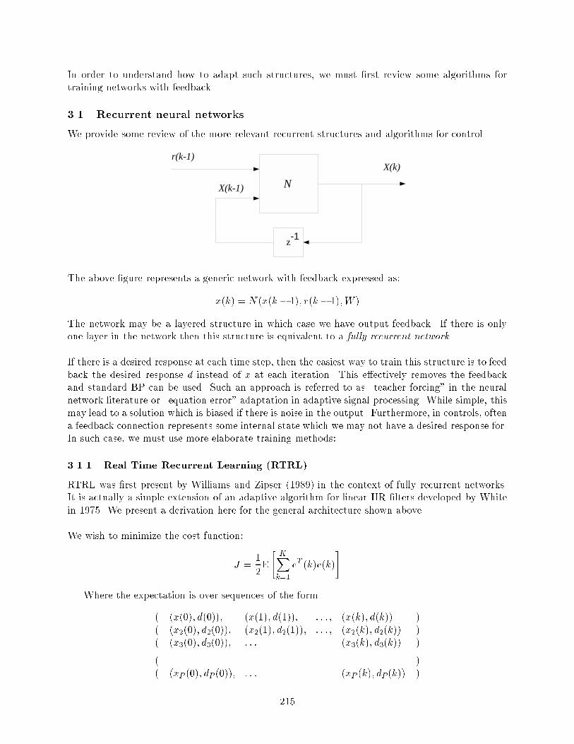
In order to understand how to adapt such structures, we must rst review some algorithms for
training networks with feedback.
3.1 Recurrent neural networks
We provide some review of the more relevant recurrent structures and algorithms for control.
N
r(k-1)X(k)
X(k-1)
z-1
The above gure represents a generic network with feedback expressed as:
x(k) = N(x(k 1); r(k 1);W )
The network may be a layered structure in which case we have output feedback. If there is only
one layer in the network then this structure is equivalent to a fully recurrent network.
If there is a desired response at each time step, then the easiest way to train this structure is to feed
back the desired response d instead of x at each iteration. This eectively removes the feedback
and standard BP can be used. Such an approach is referred to as \teacher forcing" in the neural
network literature or \equation error" adaptation in adaptive signal processing. While simple, this
may lead to a solution which is biased if there is noise in the output. Furthermore, in controls, often
a feedback connection represents some internal state which we may not have a desired response for.
In such case, we must use more elaborate training methods:
3.1.1 Real Time Recurrent Learning (RTRL)
RTRL was rst present by Williams and Zipser (1989) in the context of fully recurrent networks.
It is actually a simple extension of an adaptive algorithm for linear IIR lters developed by White
in 1975. We present a derivation here for the general architecture shown above.
We wish to minimize the cost function:
J =1
2E
"KXk=1
eT (k)e(k)
#
Where the expectation is over sequences of the form
( (x(0); d(0)); (x(1); d(1)); : : : ; (x(k); d(k)) )
( (x2(0); d2(0)); (x2(1); d2(1)); : : : ; (x2(k); d2(k)) )
( (x3(0); d3(0)); : : : (x3(k); d3(k)) )
(...
... )
( (xP (0); dP(0)); : : : (xP (k); dP(k)) )
215

Dene
e(k) =
(d(k) x(k) if 9d(k)0 else
(some outputs may have desired responses; others governed by internal states.) The update rule is
W = deT (k)e(k)
dW= 2eT (k)
dx(k)
dW
Then
dx(k)
dW| z rec(k)
=@N(k)
@x(k 1)| z Gx(k)
dx(k 1)
dW+
@N(k)
@r(k 1)
=0z | dr(k 1)
dW+@N(k)
@W| z (k)
=Iz|dW
dW
so that
rec(k) = Gx(k)rec(k 1) + (k)
with
Gx =@N(k)
@x(k 1)2 RNxNx
and
=@N(k)
@W2 RNxNW :
Then the update rule becomes
W = 2eT (k)rec(k):
Note that this is O(N2M) for M weights and N outputs. For a fully recurrent network this is
O(N4), which is not very ecient.
To calculate the necessary Jacobian terms, we observe that,
dJ(k)
dW=@JT (k)
@N(k)
dN(k)
dW= eT dN(k)
dW
dJ(k)
dx=@JT (k)
@N(k)
dN(k)
dx(k)= eT dN(k)
dx
These are found by a single backpropagation of the error. To get dN(k)dW
and dN(k)
dx(k), backprop unit
vectors e = [0 : : :010 : : :0]T .
3.1.2 Dynamic BP
This method by Narendra is an extension of RTRL.
N
r(k-1)X(k)
X(k-1)
W(z)
216

X(k 1) = W (z)X(k) (145)
where W (z) is a Linear Operator (we should really use the notation W (q)).
Example 1: Full Feedback:
)
26664(z1) 0 0 0
0 (z1) 0 0
0 0 (z1) 0
0 0 0 (z1)
3777526664X1
X2
X3
X4
37775
Example2: Tap delay line on X1.
)
26664(z1) + (z2) + (z3) + (z4) 0 : : : : : :
0 0 : : : : : :
0 0 : : : : : :
0 0 : : : : : :
3777526664X1
X2
X3
X4
37775The equation for DBP is the following modication of RTRL:
rec =dx(k + 1)
dW(146)
rec(k) = Gx(k)W (z)rec(k) + (k) (147)
(Note the mix of time-domain and \frequency" domain operators)
3.2 BPTT - Back Propagation through Time
(Werbos, Rumelhart et al, Jordan, Nguyen,...)
N(X,r,W)
r(k-1)X(k)
X(k-1)
q-1
r(0) r(1) r(2) r(N-1)
X(N)
X(0) X(1) X(2) X(3)
N N N N
Just unravel in time to get one large network.
Backprop through the entire structure.
217

Error may be introduced at nal time step or at intermediate time steps
Store 4w for each stage ! average all of them together to get a single 4w for the entire
training trajectory.
3.2.1 Derivation by Lagrange Multipliers
We present a derivation of BPTT by Lagrange Multipliers, which is a common tool for solving
N-stage optimal control problems.
We want to
minW
1
2
NXk=1
(dk Xk)T (dk Xk)
Subject to
X(k+ 1) = N(X(k); r(k);W)
Note that W acts like the control input. Next, simply adjoin the constraint to get the modied
cost function:
J =NXk=1
1
2(dk Xk)
T (dk Xk) +N1Xk=0
Tk+1[N(k)Xk+1]
=N1Xk=1
(1
2jdk Xkj2 + k+1N(k) kXk) +
1
2jdN XN j2 + T1N(0) + T
NXN
The rst constraint is that@J
@X(k)= 0
For k = N , we get
N = (dN XN)T (Terminal Condition);
For k 6= N , we get
k = (dk Xk)T + T
k+1
@N(k)
@X(k)
which is the BPTT equation that species to combine the current error with the error propagated
through the network at time k + 1.
The second optimality condition:
@J
@W=
N1Xk=0
Tk+1
@N(k)
@W= 0;
which gives the weight update formula, and explicitly says to change 4W by averaging over all
time as we argued before.
Variations
N-Stage BPTT. Just backprop a xed N stages back. This allows for an on-line algorithm.
(If N is large enough, then gradient estimate will be sucient for convergence).
1-Stage BPTT. In other words, just ignore the feedback as we saw last lecture.
218
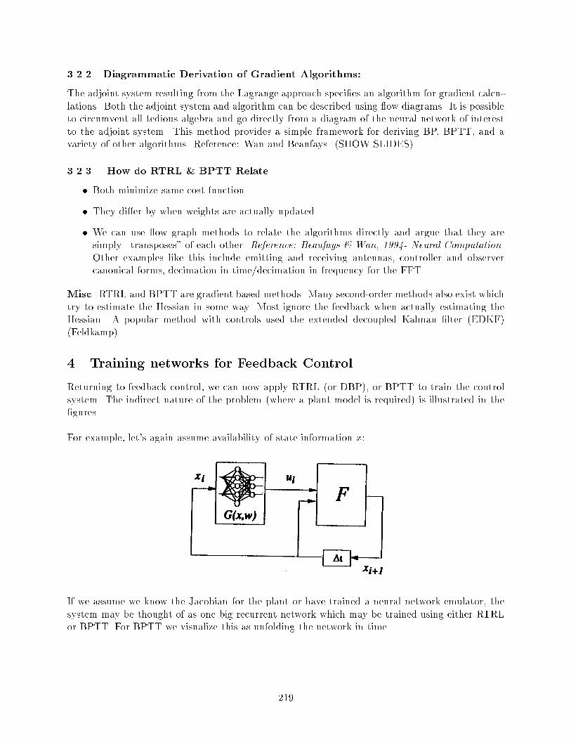
3.2.2 Diagrammatic Derivation of Gradient Algorithms:
The adjoint system resulting from the Lagrange approach species an algorithm for gradient calcu-
lations. Both the adjoint system and algorithm can be described using ow diagrams. It is possible
to circumvent all tedious algebra and go directly from a diagram of the neural network of interest
to the adjoint system. This method provides a simple framework for deriving BP, BPTT, and a
variety of other algorithms. Reference: Wan and Beaufays. (SHOW SLIDES)
3.2.3 How do RTRL & BPTT Relate
Both minimize same cost function.
They dier by when weights are actually updated.
We can use ow graph methods to relate the algorithms directly and argue that they are
simply \transposes" of each other. Reference: Beaufays & Wan, 1994- Neural Computation.
Other examples like this include emitting and receiving antennas, controller and observer
canonical forms, decimation in time/decimation in frequency for the FFT.
Misc. RTRL and BPTT are gradient based methods. Many second-order methods also exist which
try to estimate the Hessian in some way. Most ignore the feedback when actually estimating the
Hessian. A popular method with controls used the extended decoupled Kalman lter (EDKF)
(Feldkamp).
4 Training networks for Feedback Control
Returning to feedback control, we can now apply RTRL (or DBP), or BPTT to train the control
system. The indirect nature of the problem (where a plant model is required) is illustrated in the
gures.
For example, let's again assume availability of state information x:
If we assume we know the Jacobian for the plant or have trained a neural network emulator, the
system may be thought of as one big recurrent network which may be trained using either RTRL
or BPTT. For BPTT we visualize this as unfolding the network in time.
219

we simply treat every block as a Neural Network and backprop all the errors.
If we have a model with the output as a function of the states, y = h(X):
r(k-1)
X(k-1)X(k)
G F . . .
h
e(k)
y(k)
d(k)
For more complicated structures such NARMA models we still apply either BPTT or RTRL. For
example, Feldkamp's control structure uses a feedforward network with a tap delay line feed back
from the output along with locally recurrent connections at each layer.
4.1 Summary of methods for desired response
Regulators (steady-state controllers):
220

1. Model Reference (as seen before)
J = minXjjdk Xkjj2
Where dk come from some plausible model that we would like the system to emulate (e.g., a
2nd order linear model).
2. \Linear" Quadratic Regulator
J = minX
(XT
kQkXk| z
Weighting function
+ UTRkUk)| z Constraint on control effort
Eectively dk = 0 or some constant, and we weight in control eort. To modify either RTRL
or BPTT, simply view U and X as outputs:
r(k-1)
X(k-1)
X(k)
N P
q-1
u(k)
@J
@Uk= 2(Uk)
TR ! (error for U)
@J
@Xk
= 2(Xk)TQ ! (error for X)
X(k-1)
2X(k) Q
G G
q+1
2u(k) R
N P
TT
221

Final Time Problems (Terminal Control)
1. Constraint is only at nal time. Examples: Robotic arm, Truck backing.
J = min jjdN XN jj2
although one could add additional trajectory constraints (e.g. smoothness).
4.1.1 Video demos of Broom balancing and Truck backing
Comments:
Network Dimensions
Single broom 4-1
Double broom 6-10-1
Single Trailer 4-25-1
Double Trailer 5-25-1
222
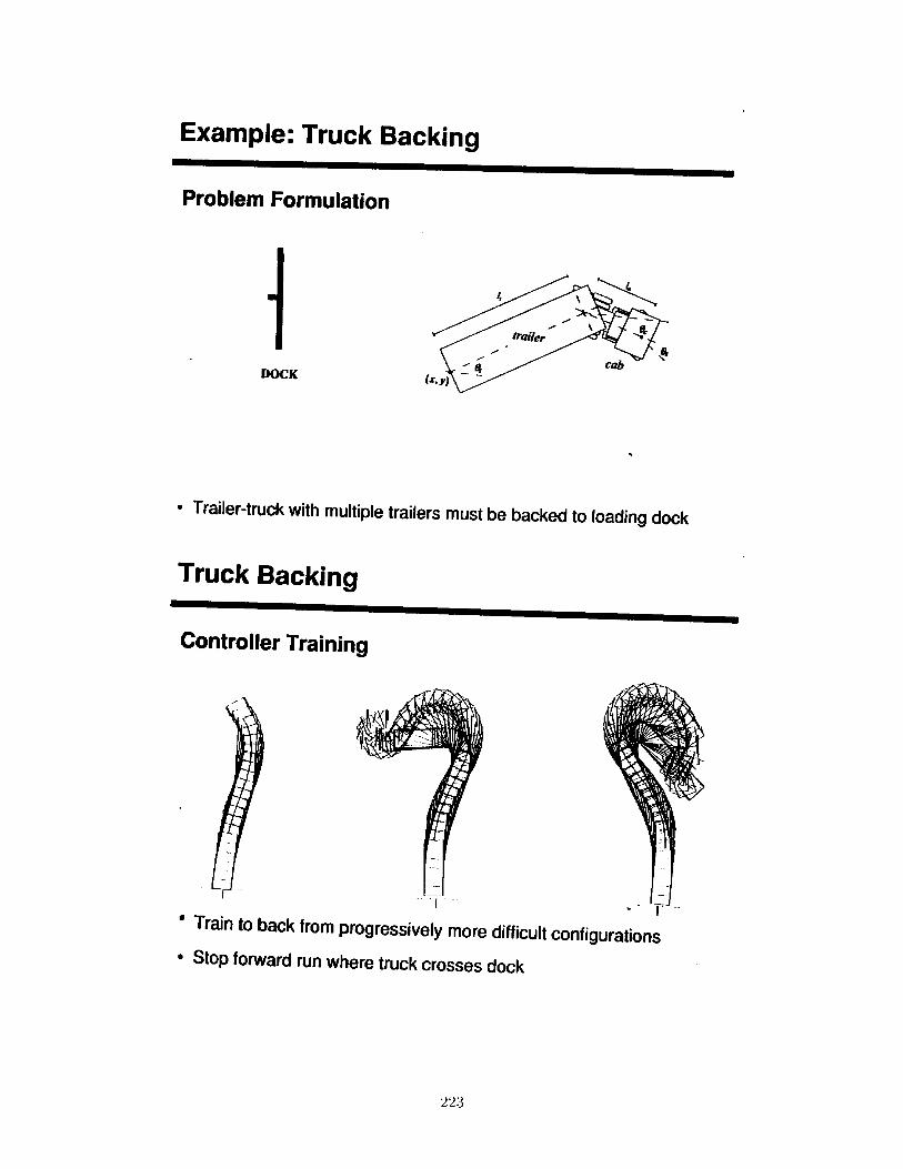
223

224

225

226

227

228

4.1.2 Other Misc. Topics
Obstacle avoidance and navigation. See slides and video.
TOBPTT (time optimal): In above problems, the nal time N is unknown (or hand picked).
We can also try to optimize over N.
J = minW;N(Xo)
E[(X;N)+
N(Xo)Xk=0
L(X(k); U(k)]
where (X;N) is the cost of nal time. The basic idea is to iteratively forward sweep,
followed by a backward error sweep, up to time a time N, which minimizes above cost for
current (Plumer, 1993).
Model Predictive control with neural networks also possible. (Pavillion uses this for process
control, also Mozer's energy control.)
4.1.3 Direct Stable Adaptive Control
Uses Radial Basis functions and Lyapunov method to adapt controller network without need for
plant model (Sanner and Slotine, 1992). This is very good work, and should be expanded on in
future notes.
4.1.4 Comments on Controllability / Observability / Stability
Controllability refers to the ability to drive the states of the systems from arbitrary initial condi-
tions to arbitrary nal states using the control input. In linear systems, this implies state feedback
is capable of arbitrarily modifying the dynamics.
Observability refers to the ability to determine the internal states of the system given only mea-
surements of the control signal and the measures plant output. For a linear system, this implies
we can estimate the states necessary for feedback control.
For a nonlinear systems:
The System X(k+1) = f(X(k); U(k)) is controllable in some region of an equilibrium point,
if the linearized system is controllable.
The same holds for observability .
Global controllability and observability for nonlinear systems are extremely dicult prove. Proofs
do not currently exist that neural networks are capable of learning an optimal control scheme,
assuming controllability, or are capable of implementing global observers.
General proofs of stability, robustness, etc. are still lacking for neural control schemes.
229

5 Reinforcement Learning
The name \Reinforcement learning" comes from animal learning theory and refers to \occurrence
of an event in proper relation to a response, that tends to increase the probability that the response
will occur again in the same situation".
We will take two dierent cracks at presenting this material. The rst takes an historical
approach and then arrives at the dynamic programming perspective. Second, we will come back
for a more detailed coverage taking \approximate" dynamic programming as a starting place.
Learning can be classied as:
Supervised Learning:
output evaluation provided
desired response encoded in cost function.
Unsupervised Learning:
no desired response given
no evaluation of output provided.
Reinforcement Learning:
no explicit desired response is given
output coarsely evaluated (reward / punish).
Examples requiring reinforcement:
Playing checkers (win/lose)
Broom balancing (crashed/balanced)
Vehicle Navigation (ok/collision/docked).
Note we already showed how to solve some of these problems using BPTT based on the Euler-
Lagrange approach. Reinforcement Learning is just another approach (based on DP).
Exploration and Reinforcement
In reinforcement learning, system must discover which outputs are best by trying dierent
actions and observing resulting sequence of rewards.
Exploration vs Exploitation dilemma:
Exploitation use current knowledge about environment and perform best action cur-
rently known
Exploration explore possible actions hoping to nd a new, more optimal strategy.
Exploration requires randomness in chosen action.
230

Σ f y
noise
Figure 35: Add randomness to a system - method 1
f Random flipBernoulli 0/1 yi=+/- 1
equivalent
Σ
Σ
noise
y
Figure 36: Add randomness to a system - method 2
Adding randomness to a system (see Figure 35 and 36). For those gures: Prfyi = 1jwi; xig = Pi.
Method 3 - Ising model
yi = 1 ;si =
Xwijxj ;
Prfyi = 1g =1
1 + exp(2si);
E[yi] = tanh(si) ;
where is the temperature parameter.
We will see that the current view of reinforcement relates to approximate dynamic programming.
While true DP explicitly explores all possible states of the system, RL must use randomness to
\explore" some region around current location in state space. Sometimes strict adhesion to this
principle makes the job more dicult than it really is.
231

Basic reinforcement structure
Classes of Reinforcement Problems:
1. Unique credit assignment
one action output
reinforcement given at every step
reinforcement independent of earlier actions and states
state independent of earlier states and actions
2. Structural credit assignment
like (I) but involves multiple action units
how to distribute credit between multiple actions
3. Temporal credit assignment (game playing, control)
reinforcement not given on every step
state dependent on earlier states and actions
how to distribute credit across sequence of actions
Class (I), (II) are easy. Class (III) is more challenging, and is what current research deals with.
Class(I) - Simple credit assignment Example:
1. Example: Adaptive Equalizers (see Figure below)
Z-1 Z-1 Z-1yks
w
\reward" every decision
w = kx(k i) ;and k = sign(sk) sk
232

\reinforces" response for next time
if we start out fair response, this method continues to get better.
Reward-Penalty:
\psuedo" desired di(t) =
(yi(t) if r(t) = +1
yi(t) if r(t) = 1dene error = yi(t) < yi(t) >
Here < yi(t) > is the expectation for stochastic units and Pi for Bernoulli units. This says to
make the current output more like the average output. Then we have
w = r(yi < yi(t) >)X :
2. Black Jack - Early example of ARP (1973 Widrow, Gupta, Maitra IEEE SMC-3(5):455-465)
Temporal problem but temporal credit problem ignored
Also called \selective boot strap"
Particular encoding makes optimal strategy linearly separable
Punish or reward all decisions equally
Weak punish / strong reward -> better convergence
Works because wins tend to result from many good decisions.
Class(II) - Structural Credit Assignment.
233

Train a model to predict E[r] for given (x,a)
Backprop through environment model to get action errors
Like plant model in control
Class(III) - Temporal Credit Assignment.
Adaptive Heuristic Critic
Critic synthesizes past reinforcements to provide current heuristic reinforcement signal to actor.
Samuel's checker programs:
Used a method to improve a heuristic evaluation function of the game of checkers during play
Best evaluation for a given move -> win/lose sequence used to determine next move
Updated board evaluations by comparing an evaluation of the current board position with
an evaluation of a board position likely to arise later in the game (make current evaluation
look like nal outcome - basic temporal credit assignment)
Improved to evaluate long term consequences of moves (tries to become optimal evaluation
function)
In one version, evaluation was a weighted sum of numerical features, update based on error
between current evaluation and predicted board position.
5.1 Temporal Credit Assignment
5.1.1 Adaptive Critic (Actor - Critic)
Adaptive critic seeks to estimate a measure of discounted, cumulative future reinforcement.
Many problems only involve reinforcement after many decisions are made.
Critic provides a step by step heuristic reinforcement signal to action network at each time
step.
The actor is just the RL terminology for the controller.
234

5.1.2 TD algorithm
Re-popularized reinforcement learning. (1983 - Sutton, Barto, Anderson)
ACE (Adaptive Critic Element) or called ASE (Associative Search Element), which is the controller.
V (t0) = E
8<:1Xt=t0
tr(t) j w; x(t)
9=;This gives the overall utility of state x(t) given current actor W with action a = N(x;W ), where
N may be a Neural Network actor). (Notation: V = J in Chapter on DP)
Critic
1. V (t) is unknown. The critic builds an estimate V (t) by interaction with the environment.
2. The critic also provide an immediate heuristic reinforcement to the actor.
(t+ 1) = r(t+ 1) + V (t+ 1) V (t)| z temporal difference
This is immediate reinforcement with temporal credit assignment.
Discounted immediate return by taking action a.
if our action takes us to a better utility then reward.
otherwise punish.
(along optimal (t+ 1) = 0, assuming no randomness).
Actor Weight Update (controller)
Dene a \weight eligibility" trace.
e(t) (not error) - analogous to (d - y)x in LMS (y is the actor a).
But don't have d, use error as before.
e(t) = (a(t) < a(t) >)x
Averaged eligibility trace
e(t) = e(t) + (1 )e(t)
Wa(t+ 1) = a(t+ 1)eij(t)
(Similar form to immediate reinforcement seen before).
235

Comment
If using Net, we need to Backprop terms through network to maintain eligibility traces for each
weight vector.
Where to get V - train critic
TD method
V = ACE(x(t);Wc(t))
where the ACE may be a Neural Net or table lookup (box-representation). Tries to predict V
based on only the current state.
Consider nding Wc to minimize (V V )2
Wc = c(V Vt) rwV| z BP term
where V is the actual future utility.
But we still need the true V.
Total weight update is
W =mXt=1
Wt =mXt=1
(V Vt)rwVt
But,
V Vt =mXk=t
(Vk+1 Vk)
Assuming Vm+1 = V
(sum of individual dierences).
W =Xt
(Xk
Vk+1 Vk)rwVt
=mXk=1
mXt=1
(Vk+1 Vk)rwVt
Rearranging terms and changing indices (k $ t),
W =mXt=0
(Vt+1 Vt)tX
k=1
rwVk| z sum of all previous
. gradient vectors.
236

But this can be done incrementally.
Wt = (Vt+1 Vt)tX
k=1
rwVk
Variations -
Discount previous gradient estimates (like RLS).
XrwVk !
tXk=1
tk rwVk| z x for single neuron
implemented as
"t = rwVt + "t1 "0 = 0
(TD())
Here's a second (easier) argument for TD():
Assume discounted future sum
V ! V (t) =1Xk=0
tr(t+ k + 1)
V (t) V (t) = rt+1 + V (t+ 1) V (t)
Assume V = V (t+ 1)
= rt+1 + V (t+ 1) V (t) = (t+ 1)
Summarizing, the TD algorithm is expressed as :
Wt critic = c(t+ 1)tX
k=1
tkrwVk ! ACE
Wt actor = a(t+ 1)e(t) ! ASE
Alternative argument: by Bellman's optimality condition,
V (t) = maxa(t)fr(t+ 1) + V (t+ 1)g
Let V ! V and ignore probability.
Error for critic with output V is
r(t+ 1) + V (t+ 1) V (t) = (t+ 1)
237

5.2 Broom Balancing using Adaptive Critic
1983 Barto, Sutton, Anderson.
Figures from: C.Anderson "Learning to Control an Inverted Pendulum using neural networks",
IEEE Control System Mag., April 1989.
Using an ML net to produce non-linear critic.
Quantizing input space and - use 0/1 representation for each bin. Binary inputs combined using
single layer.
238
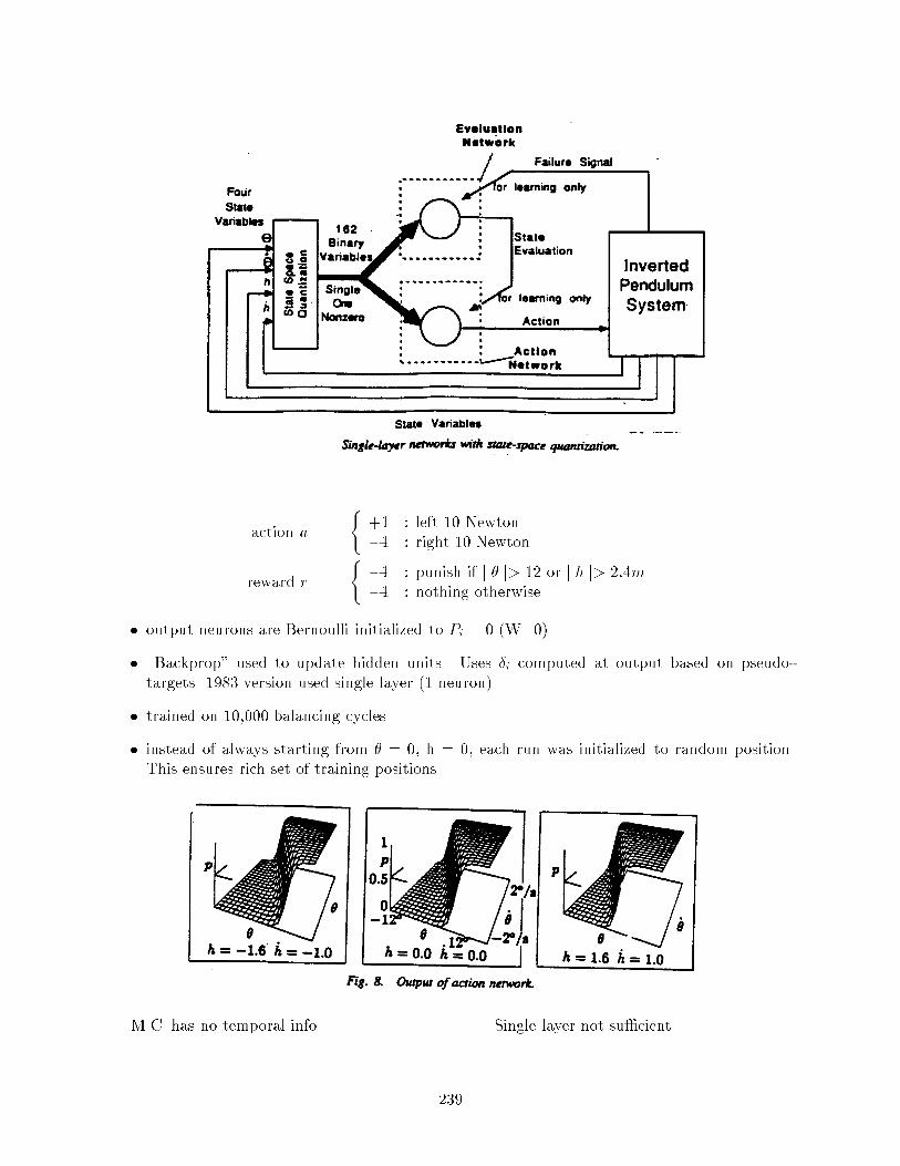
action a =
(+1 : left 10 Newton
1 : right 10 Newton
reward r =
(1 : punish if j j> 12 or j h j> 2:4m
1 : nothing otherwise
output neurons are Bernoulli initialized to Pi = 0 (W=0)
\Backprop" used to update hidden units. Uses i computed at output based on pseudo-
targets. 1983 version used single layer (1 neuron).
trained on 10,000 balancing cycles.
instead of always starting from = 0, h = 0, each run was initialized to random position.
This ensures rich set of training positions.
M.C. has no temporal info. Single layer not sucient.
239

5.3 Dynamic Programming Perspective
V (t) = E
(1Xt=0
tr(x(t); a(t)) j x0 = x(t);W
)
where W represents the current actor parameters.
Bellman's Optimality Equation from Dynamic Programming.
V (x) = maxa(t)
24r(x(t); a(t)) + X
x(t+1)
Prob(x(t+ 1) j x(t); a(t))V (x(t+ 1))
35Note
V (x) = maxW
V (x;W )
only if the model we choose to parameterize V by is powerful enough.
Aside :
V ! V , ignore probability, assume actor chooses a \good" action -
r(t+ 1) + V (t+ 1) V (t) = (t+ 1)
which is the immediate reinforcement signal for the controller, Alternatively, we can solve directly
for the control action by:
a = argmaxa(t)
hr(xt; at) +
XP (xt+1 j xt; at)V (xt+1)
iDiculty is that P as well as V must be known (need some model to do this correctly).
We thus see that we don't really need a network for the controller. However, the role of actor
to do exploration. Also, it may be advantageous during training for helping \smooth" the search,
240

and for providing \reasonable" control constrained by the parameterization of the controller.
Policy Iteration - a parameterized controller is maintained.
Value Iteration - Only the \value" function (critic) is learned, and the control is inferred from it.
5.3.1 Heuristic DP (HDP)
(Werbos and others)
X k
V
Critic
Action
Model
Plant Critic ^V
r
kX
k
kk
kX
a r
V k+1
V^
^
desired
environment
should be V*
BP this direction
also
first term in TD algorithm (just top branch)
error
X k+1
+
+
k+1V^
γ
z+1
Note that we only use critic to get dV
dxkto actually update networks.
Dual Heuristic Programming (DHP) -
Updates an estimate
(x; w) =dV
dxk
directly.
241

5.4 Q-Learning
(Watkins)
Notation: V W or QW ! where W is the current critics parameters.
We showed,
V = maxat
24r(xt; at) + Xxt+1
Prob(x(t+ 1) j xt; at)V (x(t+ 1))
35Dene
QW (xt; at) = r(xt; at) + Xxt+1
P (xt+1 j xt; at)VW (xt+1)
V = maxa
[Q(x; a)]
Bellman's Equation in Q alone
Q(xt; at) = r(xt; at) + Xat+1
P (x(t + 1) j xt; at)maxat+1
Q(xt+1; at+1
Note - max is only on the last term, thus given
a = argmaxa
[Q(x; a)]
without the need for a model !
Q-Learning Algorithm :
Q(xt; at) Q(xt; at)(1 t) + t
rt + max
at+1
Q(xt+1; at+1)
where
0 < t < 1;1Xt=1
t =1; 2t<1
Q ! Q with probability 1 if all pairs are tried innitely often.
Look up table - grows exponentially in size.
1. choose action a (with some exploration) and xt+1 is resulting state.
2. update Q
3. repeat
nal controller action is maxa Q(x; a) or an approximation.
A Neural Network may also be used to approximate the controller:
x
NN Q
a
^
242

Qdes = rt + maxat+1
Q(xt+1; at+1)
No proof for convergence.
A related algorithm is Action Dependent HDP (ADHDP) - Werbos. Uses action network output
as best at+1 - just like HDP but critic also has at as input.
5.5 Model Dependant Variations
TD, Q-Learning are model free, i.e. they don't use Prob(xt+1 j xt; at).
Several methods exist which explicitly use knowledge of a model. These are referred to as \Real
Time DP".
Example : Backgammon - Sutton's \Dyna" architecture (could also apply it to Broom Balanc-
ing).
Methods are based on approximation :
V t+1 = max
a
24r(xt; at) + Xxt+1
Prob(x(t+ 1) j xt; at)V t (xt+1)
35(with some reasonable restrictions based on current states).
V tis iteratively updated in this manner.
(TD and Q-Learning can be shown to be approximations to the RTDP methods).
5.6 Relating BPTT and Reinforcement Learning
We have seen two approaches to neural control problems which optimize a cost function over time,
BPTT and RL. How are these related? BPTT is based on the calculus of variations or Euler-
Lagrange approach, while RL is based on DP. EL and DP were our two main frameworks for
solving optimal control problems. Recall also the relation-ship derived using the HJB equations.
The in uence function (k) = @J=@u(k), or equivalently (k) = @V =@u(k). In words, the delta
terms found with backpropagation-through-time can be equated to the partial derivative of the
value function.
5.7 LQR and Reinforcement Learning
RL has the reputation of often being excruciatingly slow. However, for some problems we can help
the approach out by knowing something about the structure of the value function V . For example,
in LQR we have shown a number of times that the optimal LQ cost is quadratic in the states. In
243

fact the V function is simply the solution of a Ricatti equation. However, rather than algebraically
solving for the Ricatti equation we can use RL approaches to learn the quadratic function. A nice
illustration of this is given by Stefan Schaal at Georgia Tech., where learning pendulum balancing
is achieved after a single demonstration (SHOW TAPE on Anthropomorphic Robot Experiments).
6 Reinforcement Learning II
(Alex T. Nelson)
6.1 Review
Immediate RL: r(xt; at) is an evaluation (or reinforcement) of action at and state xt, and is
available at time t.
Delayed RL: a single value of r is available for an entire sequence of actions and states f(xt; at)g
Typical Delayed RL methods maintain an approximation, V of the optimal value function V , and
use Immediate RL methods as follows: If a : x 7! y, then the dierence, V (y) V (x) provides animmediate evaluation of the pair (x; a).
6.2 Immediate RL
We want to nd parameters w such that:
r(x; (x;w)) = r(x) 8x 2 X ;
where r(x) = maxa r(x; a) is the reinforcement for the optimal action at state x, and where (x;w)
represents the action policy parameterized by w. In other words, we want to nd a policy which
will maximize the reinforcement.
Unlike supervised learning, we don't have directed error information:
= (x;w) (x)
So . . .
1. Have to obtain weight change some other way.
2. Also, we don't know when we've converged to the correct mapping.
6.2.1 Finite Action Set
A = fa1; a2; a3; : : : ; amgDevise two functions, g(:) : X 7! <m, and M(:) : <m 7! A.
g(:) produces a merit vector for the possible actions.
M(:) selects the action with the highest merit:
(x;w) =M(g(x;w))
Since M(:) is predened, we only need to learn g(:)
244

Approximate the optimal reinforcement with r(x; v) r(x), where we write the training rule
for the parameters v in shorthand:
r(x; v) := r(x; v) + (r(x; a) r(x; v))
Notice that r(x) will approximate E[r(x; a)jx], but that this value will converge to r(x) if a is
chosen with the max selector, M(:).
The update for the merit function (kth action) is:
gk(x;w) := gk(x;w) + (r(x; ak) r(x; v)):
Problems:
1. at each x, need to evaluate all members of A2. maximum selector M(.) doesn't allow for exploration
So:
1. use stochastic action policy
2. decrease stochasticity with time (simulated annealing)
Also:
1. decrease as r ! r
2. randomize initial conditions over many trials.
6.2.2 Continuous Actions
A <Merit vectors are no longer suitable, so we need to adapt the action policy directly. There are
two basic approaches.
Stochastic: A perturbation is added for exploration.
(:) = h(:;w) + ;
where N(0; 2) The learning rule for the function approximator is:
h(x;w) := h(x;w) + [r(x; a) r(x; v)]
Which increases the probability of choosing actions with optimal reinforcement.
Deterministic: If r is dierentiable,
(x;w) := (x;w) + @r(x; a)
a
If r is unknown, use r.
The stochastic method does not suer from local maxima problems, whereas the deterministic
method is expected to be much faster because it searches systematically.
245

6.3 Delayed RL
6.3.1 Finite States and Action Sets
Assume Markovian and stationary stochastic dynamic systems; i.e.,
P (xT+1 = yjf(xt; at)gT0 ) = P (xT+1 = yjxT ; aT );
which is just Pxy(a), the probability of moving to state y from state x via action a.
Value Functions: We begin by dening the value of a policy at state x:
V (x) = E
"1Xt=0
tr(xt; (xt))
x0 = x
#;
which can be interpreted as:
V (x) = limN!1
E
"N1Xt=0
tr(xt; (xt))
x0 = x
#:
2 [0; 1) is a discount factor on future rewards. We can now dene the optimal value function
in terms of V (x):
V (x) = maxV (x) 8x
Optimal Policy: Dene optimal policy, as:
(x) = argmax
V (x) 8x 2 X ;
which is to say,
V (x) = V
(x) 8x 2 X :
Using Bellman's optimality equation,
V (x) = maxa2A(x)
24r(x; a) + Xy2X
Pxy(a)V(y)
35 ;and provided that V is known, we have a mechanism for nding the optimal policy:
(x) = arg maxa2A(x)
24r(x; a) + Xy2X
Pxy(a)V(y)
35Unfortunately, this requires the system model, Pxy(a) in addition to our approximation of
V .
Q Functions: The idea is to incorporate Pxy(a) into the approximation. Dene
Q(x; a) = r(x; a) + X
Pxy(a)V(y)
so Q = Q
=) V (x) = maxa[Q(x; a)], and
(x) = argmaxa[Q(x; a)]
246

6.4 Methods of Estimating V (and Q)
6.4.1 n-Step Truncated Return
This is a simple approximation of the value function
V [n](x) =n1X=0
r V (x; v) = E[V [n](x)]
V (x; v)! V (x) uniformly as n!1, but note that the variance of V [n](x) increases with n.
Problem: computing E[].
Solutions:
1. use V (x; v) = V [n](x) (high variance for high n)
2. use V (x; v) := V (x; v) + [V [n](x) V (x; v)] and iterate over many trials.
6.4.2 Corrected n-Step Truncated Return
We can take advantage of having an approximation of V on hand by adding a second term to the
n-step truncated return:
V (n)(x) =n1X=0
r + nV (xn; vold) V (x; vnew) = E[V (n)(x)]
Approximating E[.]:
1. use V (x; v) := V (x; v) + [V (n)(x) V (x; v)]
6.4.3 Which is Better: Corrected or Uncorrected?
Known Model Case, Using Expectation
1. Uncorrected convergence:
max jV (x; v) V (x)j nrmax
1
2. Corrected convergence:
max jV (x; vnew) V (x)j nmaxxjV (x; vold) V (x)j
This is a tighter bound.
Model Unavailable, or Expectation Too Expensive
1. If V is good, use Corrected and small n. Using Uncorrected would require large n,
resulting in higher variance.
2. If V is poor, both require large n, and the dierence is negligible.
V (n) is better
We need a way of choosing truncation length n dynamically, depending on the goodness of
V .
247

6.4.4 Temporal Dierence Methods
Consider a geometric average of V (n)'s, over all n.
V (x) = (1 )1Xn=1
n1V (n)(x)
= (1 )(V (1) + V (2) + 2V (3) + )
Using our denition of V (n) and expanding gives:
V (x) = r0 + (1 )V (x1; v) + [r1+ (1 )V (x2; v) + [r2+ (1 )V (x3; v) +
which (using r0 = r(x; (x)) ) can be computed recursively as(V (xt) = r(xt; (xt)) + (1 )V (xt+1; v) + V (xt+1)
xt := xt+1
Note that:
= 0 =) V 0(x) = r0 + V (x; v) = V (1)(x)
= 1 =) V 1(x) = r0 + V 1(x1)
=) V 1(x) = r0 + (r1+ V 1(x2)) = V (1)(x)
=) V 1(x) = V (x)
Idea: vary approximate truncation length, n, from 0 to 1 by starting with = 1 and letting
! 0 as V improves.
Problem: V takes forever to compute because of the innite sum over n.
Solution: approximate V on-line. Replace the corrected n-step estimate with:
V (x; v) := V (x; v) + [V (x) V (x; v)]: (148)
Now dene the temporal dierence as the dierence between the new prediction of the value
and the old prediction:
(x) =
new pred.z | r(x; (x)) + V (x1; v)
old pred.z | V (x; v) :
The second term in equation 148 now can be written as:
[V (x) V (x; v)] = (x) + ( )(x1) + ( )2(x2) + ;
and we can approximate equation 148 with the online update:
V (x; v) := V (x; v) + ( )(x ) (149)
if is small.
248
Note that equation 148 and 149 update V for only a single state. We can update several
states by introducing the notion of eligibility.
e(x; t) =
8><>:0 if x never visited
e(x; t 1) if x 6= xt (not currently visited)
1 + e(x; t 1) if x = xt (currently visited)
This results in an update equation for all states:
V (x; v) := V (x; v) + e(x; t)(xt) 8x 2 X (150)
Notes:
1. Reset e's before each trial.
2. Decrease during training
3. Basically the same for Q function
6.5 Relating Delayed-RL to DP Methods
Delayed Reinf. Learning Dynamic Programming
works on-line works o-line
uses subset of X uses entire state-space Xcan be model-free requires a model
time-varying stationary
There are two popular DP methods: value iteration and policy iteration. Both of these have
spawned various dRL counterparts. There are two categories of delayed RL methods: model-based
and model-free. Model-based methods have direct links to DP methods. Model-free methods are
essentially modications of the model-based methods.
6.6 Value Iteration Methods
Original DP Method: The basic idea is to compute the optimal value function as the limit of
nite-horizon optimal value functions:
V (x) = limn!1
V n(x):
To this end, we can use the recursion
V n+1(x) = max
a2A
"r(x; a) +
Xy
Pxy(a)V
n(y)
#8x
to compute V Nfor a large number N . The policy associated with any given value function
(say, V nafter an arbitrary number of iterations) is:
(x) = argmaxa2A
"r(x; a) +
Xy
Pxy(a)V
n(y)
#8x
Problem: X can be very large, making value iteration prohibitively expensive.
249

Solution: We can update V n(x) on a subset Bn X of the state-space.
Real Time Dynamic Programming: RTDP is a model-based dRL method that does this on-
line (n is system time) and Bn includes the temporal neighbors of xn.
Q-Learning: this is a model-free dRL approach to value-iteration. As described in section 3, the
idea is to incorporate the system model into the approximation. Again the update rule for
the Q-function is:
Q(x; a; v) := r(x; a) + Xy
Pxy maxb2A(y)
Q(y; b; v): (151)
However, this update relies on a system model. We can avoid this by looking only at the
Q-function of the state that the system actually transitions to (say, x1):
Q(x; a; v) := r(x; a) + maxb2A(x1)
Q(x1; b; v): (152)
To approximate the averaging eect found in equation 151, we can use an averaging update
rule:
Q(x; a; v) := (1 )Q(x; a; v) +
"r(x; a) + max
b2A(x1)Q(x1; b; v)
#: (153)
The Q-learning algorithm consists of repeatedly (1) choosing an action a 2 A, (2) applyingequation 153, and (3) updating the state x := x1.
The choice of action in step(1) can be greedy with respect to Q, or can be made according
to some stochastic policy in uenced by Q, to allow for better exploration.
6.6.1 Policy Iteration Methods
Whereas value iteration methods maintain an explicit representation of the value function, and
implements a policy only in association with the value function, policy iteration methods maintain
an explicit representation of the policy.
Original DP Method: The idea is that if the Q-function for a policy is known, than we can
improve on it in the following way:
(x) = arg maxa2A(x)
Q(x; a) 8x; (154)
so that the new policy is at least as good as the old policy . This is because the Q(x; a)
gives the value of rst choosing action a, and then following policy . The steps of policy
iteration are:
1. Start with a random policy and compute V .
2. Compute Q.
3. Find using equation 154.
4. Compute V .
5. Set := and V := V .
6. Go to step 2 until V = V in step 4.
Problem: It is very expensive to recompute V at each iteration. The following method
gives an inexpensive approximation.
250

Actor-Critic: This is a model-free dRL method (there isn't a model-based dRL counterpart to
policy iteration). The \actor" is a stochastic policy generator, and the \critic" is a value-
function estimator. The algorithm is as follows:
1. Select action a stochastically according to the current policy, a = (x).
2. (x) = r(x; a) + V (x1; v) V (x; v) serves as the immediate reinforcement.3. Update the value estimator, V (x; v) := V (x; v) + (x).
4. Update the deterministic part of the policy generator, gk(x;w) := gk(x;w) + (x)
where k 3 a = ak is the index of the action selected.
5. Repeat.
6.6.2 Continuous Action Spaces
So far the assumption has been that there are only a nite number of actions for the policy generator
to choose from. If we now consider the case of continuous action spaces, the problem becomes much
more dicult. For example, even value-iteration methods must maintain a policy generator because
the max operation becomes nontrivial. The general approach is to update the policy generator by
taking the partial derivative of the Q-function (or Q) with respect to action a. This is a gradient
ascent approach, which adjusts the policy in the direction of increasing utility; it is comparable to
the immediate RL methods for continuous action spaces.
7 Selected References on Neural Control
(Books)
1. Reinforcement Learning, R. Sutton, A. Barto, MIT Press, 1998.
2. Neural Networks for Control, edited by W.T Miller, R. Sutton, P. Werbos. MIT Press, 1991.
3. Handbook of intelligent control : fuzzy, neural, and adaptive approaches, edited by David A.
White, Donald A. Sofge, Van Nostrand Reinhold, 1992.
4. Neuro-dynamic programming, Dimitri P. Bertsekas and John N. Tsitsiklis, Athena Scientic,
Belmont, 1997.
(Articles)
1. A. Barto, R. Sutton, A. Anderson., Neuronlike elements that can solve dicult learning
control problems. IEEE Transactions Systems, Man, and Cybernetics, 40:201-211, 1981.
2. S. Keerthi, B. Ravindran. A tutorial Survey of Reinforcement Learning. Available by request
3. Narendra, K, and Parthasarathy, K. 1990. Identication and control of dynamic systems
using neural networks. IEEE Trans. on Neural Networks, vol. 1, no. 1, pages 4-27.
4. Narendra, K, and Mukhopadhyay, S. Adaptive Control of Nonlinear Multivariable Systems
Using Neural Networks. Neural Networks, Vol. 7, No. 5., 1994.
251

5. Nguyen, D., and Widrow, B. 1989. The truck backer-upper: an example of self-learning in
neural networks, In Proceedings of the International Joint Conference on Neural Networks,
II, Washington, DC, pages 357-363.
6. Plumer, E. 1993. Optimal Terminal Control Using Feedforward Neural Networks. Ph.D.
dissertation. Stanford University.
7. G. Puskorius and L. Feldkamp. Neural control of Nonlinear Dynamic Systems with the
Kalman Filter Trained Recurrent Networks. IEEE Transactions on Neural Networks, Vol. 5.,
No. 2, 1994.
8. R. Sanner, J. Slotine. Gaussian Networks for Direct Adaptive Control. IEEE Transaction on
Neural Networks, Vol. 3., No. 6., Nov. 1992.
9. Williams, R., and Zipser D. 1989. A learning algorithm for continually running fully recurrent
neural networks. Neural Computations, vol. 1, pages 270-280.
10. Wan, E., and Beaufays, F. 1994. Network Reciprocity: A Simple Approach to Derive Gra-
dient Algorithms for Arbitrary Neural Network Structures. WCNN'94, San Diego, CA., vol
III, June 6-9, pages 87-93.
8 Videos
(List of Videos shown in class)
1. ALVINN - Dean Pomerleau, CMU
2. Intelligent Arc Furnace - Neural Applications corp,
3. Trucks and Brooms - Bernard Widrow, Stanford University,
4. Artical Fishes - Demitri Terzopolous, Toronto.
5. Anthropomorphic Robot Experiments - Stefan Schaal, Georgia Tech.
6. Catching - Slotine.
252
Part IX
Fuzzy Logic & Control
1 Fuzzy Systems - Overview
Fuzzy Methods are rmly grounded in the mathematics of Fuzzy Logic developed by Lofti
Zadeh (1965).
Very popular in Japan (great buzz-word). Used in many products as decision making elements
and controllers.
Allows engineer to quickly develop a smooth controller from an intuitive understanding of
problem and engineering heuristics.
Are dierent from and complementary to neural networks.
Possible over-zealous application to unsuitable problems.
Typically the intuitive understanding is in the form of inference rules based on linguistic variables.
Rule based
An example might be a temperature controller: If the break temperature is HOT and the
speed is NOT VERY FAST, then break SLIGHTLY DECREASED.
A mathematical way to represent vagueness.
Dierent from Probability Theory.
An easy method to design adequate control system.
When to use Fuzzy Logic:
When one or more of the control variables are continuous.
When an adequate mathematical model of the system does not exist or is to expensive
to use.
When the goal cannot be expressed easily in terms of equations.
When a good, but not necessarily optimal, solution is needed.
When the public is still fascinated with it!
2 Sample Commercial Applications
Fujitec / Toshiba - Elevator : Evaluates passenger trac, reduces wait time.
Maruman Golf - Diagnoses golf swing to choose best clubs.
Sanyo Fisher / Canon - Camcorder focus control: Chooses best lighting and focus with many
subjects.
253

Matsushita - Washing Machine : Senses quality / quantity of dirt, load size, fabric to adjust
cycle. Vacuum Cleaner : Senses oor condition and dust quantity to adjust motor. Hot water
heater : Adjusts heating element by sensing water temperature and usage rate.
Mitsubishi - Air conditioner : Determines optimum operating level to avoid on/ o cycles.
Sony - Television : Adjusts screen brightness, color, contrast. Computer : Handwritten OCR
of 3000 Japanese characters.
Subaru - Auto Transmission: Senses driving style and engine load to select best gear ratio. (
Continuum of possible gears!)
Saturn - Fuzzy Transmission.
Yamaichi Securities - Stocks: Manage stock portfolios (manages $350 million).
3 Regular Set Theory
We dene a `set' as a collection of elements. Example:
A = fx1; x2; x3g
B = fx3; x4; x5g
We can thus say that a certain thing is an element of a set, or is a member of a set.
x1 2 A ; x3 2 B
We can also speak of `intersection' and `union' of sets.
A [B = fx1; x2; x3; x4; x5g
A \ B = fx3g
\Fuzzy people" call the set of all possible \things" (all X) the universe of discourse.
The complement is A = fxi j xi =2 Ag
\Membership" is a binary operation. either x 2 A or x =2 A.
X
A AA
B
254

4 Fuzzy Logic
In Fuzzy Logic we allow membership to occur in varying degrees.
Instead of listing elements, we must also dene their degree of membership .
A membership function is specied for each set.
fA(x) : X ! [0; 1] degree of membership
Example:
X
f A
X ! range of possible members or input values, typically subset of R.
If fA(x) = f0; 1g then we have regular set theory.
Typically we describe a set simply by drawing the activation function (membership function).
A B
1
fA(1:0) = 0:4; fB(1:0) = 0:1
1.0 `belongs' to sets A and B in diering amounts.
4.1 Denitions
Fuzzy Logic developed by Zadeh shows that all the normal set operations can be given precise
denitions such that normal properties of set theory still hold.
Empty set
A = if fA(x) = 0 8 x X
Equality
A = B if fA(x) = fB(x) 8 x X
255

Complement
Ac has f cA= 1 fA(x)
Containment or Subset
A B if fA(x) fB(x) 8 x X
Union
fA[B(x) = max [fA(x); fB(x)] 8 x X
= fA [ fB
This is equivalent to the `Smallest set containing both A and B'.
Intersection
fA\B(x) = min [fA(x); fB(x)] 8 X
= fA \ fB
This is the `Largest set contained in both A and B'.
4.2 Properties
A number of properties (set theoretical and algebraic) have been shown for Fuzzy Sets. A
few are :
Associative
(A\ B) \ C = A \ (B \ C)
(A[ B) [ C = A [ (B [ C)
Distributive
C \ (A [B) = (C \A) [ (C \B)
C [ (A \B) = (C [A) \ (C [B)
De Morgan
(A [ B)c = Ac \Bc
(A \ B)c = Ac [Bc
256

4.3 Fuzzy Relations
We can also have Fuzzy relations of multiple variables.
In regular Set theory, a `relation' is a set of ordered pairs i.e,
A = x y = f(5; 4); (2; 1); (3; 0); : : :etcg
We can have Fuzzy relations by assigning a `degree of correctness" to the Logical statement
and dene membership functions in terms of two variables.
fA(10; 9) = 0; fA(100; 10) = 0:7; fA(100; 1) = 1:0
4.4 Boolean Functions
In a real problem, x would represent a real variable (temperature) and each set a Linguistic Premise
(room is cold).
Example, let t and P be variables representing actual temperature and pressure.
Let A be the premise \temperature is hot"
Let B be \pressure is normal".
Assume the following membership functions.
A
1
0 t
B
1
0 p
"temperature hot AND pressure normal" is a fuzzy relation given by the set
fAAND Bg = C1 = fA \Bg
fC1(t; P ) = min [fA(t); fB(P )] 8 t, P
For OR,
fAORBg = C2 = fA [Bg
fC2(t; P ) = max [fA(t); fB(P )] 8 t,P
For NOT,
fNOT Ag = C3 = Ac
fC3(t; P ) = 1 fA(t) 8 t
Note, the resulting fuzzy relation is also a fuzzy set dened by a membership function.
257

4.5 Other Denitions
Support and cross over.
support
.5cross-overpoint.
Singleton
x
4.6 Hedges
Modiers: not, very, extremely, about, generally, somewhat..
4 5.5 6
Tallvery tall
U ← U [X] n >1A A
n
4 5.5 6
somewhat tall
4 5.5 6
definitely tall
258

5 Fuzzy Systems
Fuzzier
Each Sensor input is compared to a set of possible linguistic variables to determine
membership.
Provides \Crisp" values
Warm
22 degrees
22 degrees
Cool
.25
.67
Process Rules (Fuzzy Logic)
Each rule has an antecedent statement with an associated fuzzy relation. Degree of
membership for antecedent is computed. - Fuzzy Logic.
IF (ANTECEDENT) THEN (CONSEQUENCE).
259

Defuzzier
Each rule has an associated action (consequence) which is also a fuzzy set or linguistic
variable such as 'turn right slightly'.
Defuzzication creates a combined action fuzzy set which is the intersection of output
sets for each rule, weighted by the degree of membership for antecedent of the rule.
Converts output fuzzy set to a single control value.
This defuzzication is not part of the 'mathematical fuzzy logic' and various strategies
are possible.
We introduce several Defuzzication possibilities later.
Design Process - Control designer must do three things:
1. Decide on appropriate linguistic quantities for inputs and outputs.
2. Dene a membership function (fuzzy sets) for each linguistic quantity.
3. Dene the inference rules.
5.1 A simple example of process control.
Sensor Inputs : 1. Temperature, 2. Pressure.
Actuator Outputs: 1. Value setting.
We must rst decide on linguistic variables and membership functions for fuzzy sets.
Next, we choose some rules of inference
if P = H and t = C then V = G (1)
260

if P = H and t = W then V = L (2)
if P = N then V = Z (3).
This is the same as
if P = N and "1" then V = Z
\Karnaugh Map"
Fuzzify - Infer - Defuzzify
261

5.2 Some Strategies for Defuzzication
Center of Mass
If B? is the composite output Fuzzy set,
y0 =
RyfB?(y) dyRfB?(y) dy
This is probably the best solution, and best motivated from fuzzy logic, but is hard to
compute.
Peak Value
y0 = argmaxyfB?(y)
This may not be unique.
Weighted Maximums
For each rule there is a Bi and an activation degree for antecedent wi.
y0 =wimaxy fBi
(y)
wi
functions of inputs.
Can also have outputs be dierent functions of the original inputs.
y0 = wi i(1 : : :n)
wi
5.3 Variations on Inference
Inference
Mamdani - minimum
Larson - product
Composition
Maximum (traditional method)
Sum (weighted and/or normalized)
262
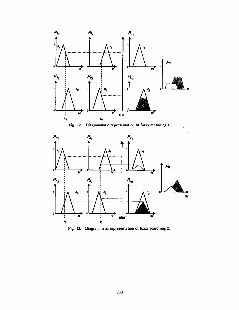
263

5.4 7 Rules for the Broom Balancer
5.5 Summary Comments on Basic Fuzzy Systems
Easy to implement (if number of inputs are small).
Based on rules which may relate directly to understanding of problem.
Produces smooth mapping automatically.
May not be optimal.
Based on designer's heuristic understanding of the solution.
Designer may have no idea what inference rules may be.
Extremely tedious for large inputs.
Often a conventional controller will work better.
Cautions: There is a lot of over-zealousness about Fuzzy Logic (buzz - word hype). There is
nothing magical about these systems. If conventional controller works well, don't toss it out.
264

6 Adaptive Fuzzy Systems
Adaptive fuzzy systems use various ad hoc techniques which attempt to:
Modify shape and location of fuzzy sets.
Combine or delete unnecessary sets and rules.
Use unsupervised clustering techniques.
Use \neural" techniques to adapt various parameters of the fuzzy system.
6.1 Fuzzy Clustering
6.1.1 Fuzzy logic viewed as a mapping
Y
X
Y
X
Example: If X is NS then Y is PS.
265
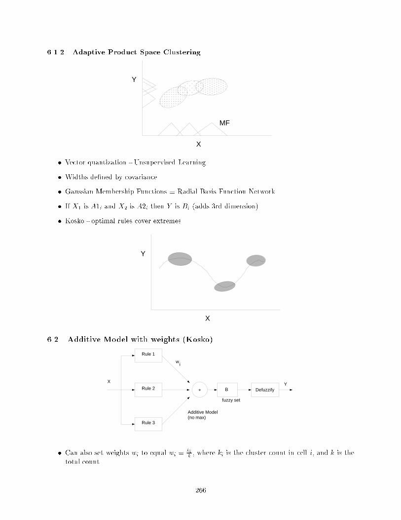
6.1.2 Adaptive Product Space Clustering
Y
X
MF
Vector quantization - Unsupervised Learning.
Widths dened by covariance.
Gaussian Membership Functions Radial Basis Function Network.
If X1 is A1i and X2 is A2i then Y is Bi (adds 3rd dimension).
Kosko - optimal rules cover extremes
Y
X
6.2 Additive Model with weights (Kosko)
Rule 1
Rule 2
Rule 3
+ B Defuzzify
X
fuzzy set
Additive Model (no max)
Y
wi
Can also set weights wi to equal wi =ki
k, where ki is the cluster count in cell i, and k is the
total count.
266

If we threshold this to wi = 0=1 which implies adding or removing rule.
Additive Fuzzy Models are \universal approximators".
6.3 Example Ad-Hoc Adaptive Fuzzy
Adaptive Weights
Weights initially set to 1 and then adapted. Truth of premise (0 to 1) reduced as w ! 0.
Adaptation can be supervised (like BP) or some reinforcement method (punish/reward weights
based on frequency of rules that re).
Adaptive Membership function support
Example:
If e = y d is positive the the system is over-reacting thus narrow regions of rules that red.
If e is negative Widen regions.
(Restrict amount of overlap to avoid instabilities)
6.4 Neuro-Fuzzy Systems
Make Fuzzy systems look like Neural Net and then apply any of the learning algorithms.(BP, RTBP,
etc).
267

6.4.1 Example: Sugene Fuzzy Model
if X is A and Y is B then Z = f(x; y).
Layer 1 - MFs
MFAi(x) =1
1 + [(xciai
)2]bi
) bell shape function parameterized by a; b; c.
Layer 2 - AND - product or soft min
soft min(x; y) = xekx + yeky
ekx + eky
Layer 3 - Weight Normalization
Layer 4 = wi(pix+ qiy + ri)
Layer 5 = wifi
Network is parameterized by ai; bi; ci; pi; qi; ri. Train using gradient descent.
In general replace hard max/min by soft max/ min and use BP,RTRL, BPTT, etc.
268

6.4.2 Another Simple Example
a11 a12 a1(m-1)
Membership functions:
U1i =
8>><>>:x1a1(i1)
a1ia1(i1)a1(i1) < x1 < a1i
a1(i+1)x1a1(i+1)ai1
a1i x1 a1(i+1)
0 otherwise
(155)
if U1i AND U2j then ....
Constraint a11 < a12 < a1m
AND - Product Rule
Defuzzication - Weighted Average
Y =Xij
(U1iU2j)wij
Gradient descent on error:
Error =1
2(Yk dk)2
@E
@wij
=Xk
(Yk dk)(U1iU2j)
@E
@a1i=Xj
Xk
(Yk dk)(i+1Xl=i1
U1iwij)
7 Neural & Fuzzy
In 1991 Matsushita Electronics claimed to have 14 consumer products using both neural networks
and fuzzy logic.
269

7.1 NN as design Tool
Neural Net outputs center locations and width of membership functions.
7.2 NN for pre-processing
Output of Neural Net is "Predicted Mean Vote" - PMV, and is meant to be an index of
comfort.
This output is fed as control input to a fuzzy controller.
Example: Input to NNet is image. Output of net in classication of stop sign / no stop sign
which goes as input to Fuzzy logic.
270

7.3 NN corrective type
Example: Hitachi Washing Machine, Sanyo Microwave.
Fuzzy designed on original inputs.
NN added later to handle additional inputs and avoid redesigning with too many inputs and
membership functions.
7.4 NN for post-processing
FuzzyLogic
NN control
NN Control
Input Low Level Control
Fuzzy for higher level logic and NN for low level control.
Example: Fuzzy determines ight high-level commands, neural implements them.
Example: Sanyo fan - Points to holder of controller. Fuzzy - 3 infrared sensors used to
compute distance. Neural - given distance & ratio of sensor outputs are used to command
direction.
7.5 Fuzzy Control and NN system ID
FuzzyLogic
InputPlant
NN IDerror
Use NNet for system ID which provides error (through BP) to adapt Fuzzy controller.
271

8 Fuzzy Control Examples
8.1 Intelligent Cruise Control with Fuzzy Logic
R. Muller, G. Nocker, Daimler-Benz AG.
272

8.2 Fuzzy Logic Anti-Lock Brake System for a Limited Range Coecient of
Friction Surface
D. Madau, F. Yuan, L. Davis, L. Feldkamp, Research Laboratory, Ford Motor Company.
273

274

9 Appendix - Fuzziness vs Randomness
(E. Plumer)
Fuzzy logic seems to have the same \ avor" as probability theory. Both attempt to describe
uncertainty in certain events. Fundamentally, however, they are very dierent. For an excellent
discussion on the dierences and implications thereof, read (B. Kosko, Neural networks and fuzzy
systems: A dynamical systems approach to machine learning, Prentice-Hall, 1992, chapter 7). It
would seem that we can make the following identications and use probability theory to describe
fuzzy logic:
Fuzzy Logic ? Probability Theory
fuzzy set () random variable
membership function, fA(x) () probability density, pA(x)
element of fuzzy set () value of random variable
As we shall see, this won't work. Before waxing philosophical on the dierences, we note a few
problems with using probability theory. Recalling basics of probability theory (see M. Gray and
L. Davisson, Random processes: A mathematical approach for engineers, Prentice-Hall, 1986) we
dene a probability space (;F; P ) as having three parts:
1. Sample Space, | collection of points or members. Also called \elementary outcomes."
2. Event Space, F | Nonempty collection of subsets of . Also called a sigma algebra of .
This set must obey the following properties: (1) if F 2 F, then F c 2 F, where F c = f! : ! 2; ! 62 Fg is the compliment of F ; (2) for nite (or countably innite) number of sets Fi, we
haveSiFi 2 F.
3. Probability Measure, P | assignment of a real number , P (F ) to every member of the sigma
algebra such that P obeys the following axioms of probability: (1) for all F 2 F, P (F ) 0;
(2) for disjoint sets Fi ( i.e. i 6= j implies Fi \ Fj = ;), we have P (SiFi) =
PiP (Fi).
A random variable is simply a mapping from the event space to the real numbers X : F! <. Theseproperties must hold in order to have a probability space and to be able to apply probability theory.
Thus, a probability space has at its root a set which obeys regular set theory. Built upon this
set is the probability measure describing the \randomness." On the other hand, in fuzzy logic, the
basic notion of a set and of all set operations and set properties is redened. Furthermore, fuzzy sets
and membership functions do not satisfy the axioms of probability theory. As an example, recall
that for a probability density function pX(x), we must have 0 pX(x) 1 andRxpX(x) dx = 1.
However, for membership functions, although 0 fA(x) 1, the value ofRxfA(x) dx can be
anything! Also, consider this very profound statement: A \ Ac = ; which states that a set and
its compliment are mutually exclusive. This certainly holds true for the event space underlying a
probability space. However, in fuzzy logic this is no longer true! A \ Ac has membership function
fA\Ac(x) = min [fA(x); 1 fA(x)] which is clearly not identically zero. Moral: probability theory
is not adequate to describe fuzzy logic.
We can also provide a few intuitive reasons why \randomness" and \fuzziness" are not the same
thing. To quote Kosko:
275

Fuzziness describes event ambiguity. It measures the degree to which an event occurs,
not whether it occurs. Randomness describes the uncertainty of event occurrence. An
event occurs or not, . . . The issue concerns the occurring event: Is it uncertain in any
way? Can we unambiguously distinguish the event from its opposite? [pp. 265].
Basically probability theory accounts for an event occurring or not occurring but doesn't permit
an event to partially occur.
Underlying probability theory is the abstract idea of some type of \coin toss experiment" which
chooses one of the elements of F as the event. The measure P describes the likelihood of any
particular event occurring and the random variable X maps the event to some output number x.
In fuzzy logic, there is no randomness, no notion of an underlying experimental coin toss, and no
uncertainty of the outcome.
A further contrasting can be made as follows: In fuzzy logic, each real value (such as T = 50C)
is associated, in varying degrees, with one or more possible fuzzy sets or linguistic variables (such
as \T is hot" or \T is very hot"). The membership function measures the degree to which each
fuzzy set is an \attribute" of the real value. In probability theory, on the other hand, the roles are
reversed. A real value does not take on a random variable, rather, a random variable takes on one
of a number of possible real values depending on the outcome of the underlying experiment.
Beyond simply describing and approach to designing control systems, \fuzziness" proposes a
completely dierent way of explaining uncertainty in the world. As Kosko points out in his book,
for example:
Does quantum mechanics deal with the probability that an unambiguous electron
occupies spacetime points? Or does it deal with the degree to which an electron, or an
electron smear, occurs at spacetime points? [pp. 266].
More fun philosophical examples are given in the rest of chapter 7 of Kosko's book.
276

Part X
Exercises and Simulator
Home work 1 - Continuous Classical Control
Home work 2 - Digital Classical Control
Home work 3 - State-Space
Home work 4 - Double Pendulum Simulator - Linear SS Control
Midterm
Double Pendulum Simulator - Neural Control/BPTT
Double Pendulum Simulator Documents
277

0.1 System description for double pendulum on a cart
u
θ1
θ2
0 x
System parameters
l1 = length of rst stick (156)
l2 = length of second stick (157)
m1 = mass of rst stick (158)
m2 = mass of second stick (159)
M = mass cart (160)
States
x = position of the cart (161)
_x = velocity of cart (162)
1 = angle of rst stick (163)
_1 = angular velocity of rst stick (164)
2 = angle of second stick (165)
_2 = angular velocity of second stick (166)
Control force
u = force (167)
278

Dynamics
Using a Lagrange approach, the dynamic equations can be written as:
(M +m1 +m2)x (m1 + 2m2)l1 1 cos 1 m2l2 2 cos 2 (168)
= u+ (m1 + 2m2)l1 _12sin 1 +m2l2 _2
2sin 2 (169)
(m1 + 2m2)l1x cos 1 + 4(m1
3+m2)l1
2 1 + 2m2l1l2 2 cos(2 1) (170)
= (m1 + 2m2)gl1 sin 1 + 2m2l1l2 _22sin(2 1) (171)
m2xl2 cos 2 + 2m2l1l2 1 cos(2 1) +4
3m2l2
2 2 (172)
= m2gl2 sin 2 2m2l1l2 _12sin(2 1) (173)
The above equations can be solved for x, 1 and 2, to form a state-space representation.
279

0.2 MATLAB les
MATLAB scripts for the simulation of the double inverted pendulum
dbroom.m:
Main scripts that designs and graphically implements linear control of
the double pendulum. Just type "dbroom" from MATLAB to run it. The
script can be edited to change initial conditions and model
specifications. The script designs the control law for the current
model specifications. Functions from the controls toolbox are
necessary.
Functions called by dbroom.m
dbroom_figs.m - Plots responses of simulation
dbroom_init.m - Initializes graphics windows
dbroom_lin.m - Linearizes the nonlinear model for given parameters
dbroom_plot.m - Graphic plot of system for current state
dbroom_sim.m - Nonlinear state-space simulation of double pendulum
dbroom_view.m - Graphic prompt for viewing figures
broom.ps : system definitions and dynamics.
Eric A. Wan
Oregon Graduate Institute
Snapshot of MATLAB window:
−3.75 3.75
280

% Double Inverted Pendulum with Linear Controller
%
% Eric Wan, Mahesh Kumashikar, Ravi Sharma
% PENDULUM MODEL SPECIFICATIONS
Length_bottom_pendulum = .5;
Length_top_pendulum = 0.75;
Mass_of_cart = 1.5;
Mass_of_bottom_pendulum = 0.5;
Mass__top_pendulum = 0.75;
pmodel = [Length_bottom_pendulum Length_top_pendulum Mass_of_cart
Mass_of_bottom_pendulum Mass__top_pendulum] ;
% INITIAL STATE
Cart_position = 0;
Cart_velocity = 0;
Bottom_pendulum_angle = 20; % degrees % +- 9 max
Bottom_pendulum_velocity = 0;
Top_pendulum_angle = 20; % degrees
Top_pendulum_velocity = 0;
% Random starting angles for fun
%Bottom_pendulum_angle = 15*(2*(rand(1)-.5));
%Top_pendulum_angle = 15*(2*(rand(1)-.5));
u = 0; % initial control force
deg = pi/180;
x0 = [Cart_position Cart_velocity Bottom_pendulum_angle*deg
Bottom_pendulum_velocity*deg Top_pendulum_angle*deg Top_pendulum_velocity*deg];
% TIME SPECIFICATIONS
final_time = 10; % seconds
dt= 0.01; % Time for simulation step
DSample = 2; % update control every Sample*dt seconds
T = dt:dt:final_time;
steps = length(T);
plotstep = 4; % update graphics every plotstep time steps
%To record positions and control force.
X = zeros(6,steps);
U = zeros(1,steps);
% setup beginning of demo
281

dbroom_init
%%%%%%%%%%%%%%%%%%%%%%%%%%%%%%%%%%%%%%%%%%%%%%%%%%%%%%%%%%%%%%%%%%%%%%%%%%
% DESIGN LINEAR CONTROLLER
% Obtain a linear state model
[A,B,C,D] = dbroom_lin(pmodel,0.001);
% form discrete model
[Phi,Gam] = c2d(A,B,DSample*dt);
%Design LQR
Q = diag([50 1 100 20 120 20]);
K = dlqr(Phi,Gam,Q,1);
% Closed loop poles
% p = eig(Phi - Gam*K)
%%%%%%%%%%%%%%%%%%%%%%%%%%%%%%%%%%%%%%%%%%%%%%%%%%%%%%%%%%%%%%%%%%%%%%%%%%
% Simulate controlled pendulum
% Plots initial pendulum state
fall = dbroom_plot(x0,u,0,f1,1,pmodel);
drawnow;
fprintf('\n Hit Return to begin simulation \n')
pause
x = x0'; i = 1;
while (i<steps) & (fall ~= 1),
i = i+1;
% Update Control force
if rem(i,DSample) <= eps, % Apply control once in DSample time steps.
u = -K*x; % Linear control law
end
% UPDATE STATE
% state simulation based on Lagrange method
x = dbroom_sim(x,u,pmodel,dt);
% PLOT EVERY plotstep TIMESTEPS
if rem(i,plotstep) <= eps
fall = dbroom_plot(x,u,i*dt,f1,0,pmodel);
end
282

% SAVE VALUES
X(:,i) = x;
U(:,i) = u;
end
% graph responses
dbroom_view
283


