COMINVEST · PM High Alpha · Folie 1
Consistent Return Estimates-
The Black-Litterman Approach
Frankfurt MathFinance Workshop 2005
Dr. Werner Koch, CEFACOMINVEST
PM High Alpha / Portfolio Construction- April 2005 -
COMINVEST · PM High Alpha · Folie 2 / 2 / PMα
The Black-Litterman ApproachConsistent asset return estimates - saving classical mean/variance...
Abstract
In asset management, the forecast of asset returns is essential within the investment process. Inthis context, the Black-Litterman approach (1992) yields consistent asset return forecasts as aweighted combination of (strategic) market equilibrium returns and (tactical) subjective forecasts(”views”). The Black-Litterman formalism allows to implement both absolute views (return levels)and relative views (outperforming vs. underperforming assets) for selected assets investigatedunder „core competence“. For any particular view, individual confidence levels for the returnestimates have to be specified. The formalism spreads these informations consistently across allassets in the portfolio. The BL-revised returns then serve as a consistent input for mean-varianceportfolio optimisation procedures, thus allowing for the implementation of additional constraints.It turns out that BL-optimized portfolios overcome some well-known Markowitz insufficiencies asunrealistic sensitivity to input factors or extreme portfolio weights. The BL process will beintroduced both from its theoretical background and its implementation in practice.
Dr. Werner Koch Frankfurt, March 2005COMINVEST Asset Management
[email protected] Last update: March 2005
Data source: DataStream

COMINVEST · PM High Alpha · Folie 3 / 3 / PMα
- The c.p. world ofcore competences -
Opinion Opinion
Opinion
Opinion
Opinion
Opinion
Opinion
Opinion Committee
Quant tool
RESEARCH PORTFOLIO CONSTRUCTION
- The portfolio context:Thinking in terms of correlations -
or
Investment Process: Opinions & Portfolio Context
c.p. = ceteribus paribus
Opinion
COMINVEST · PM High Alpha · Folie 4 / 4 / PMα
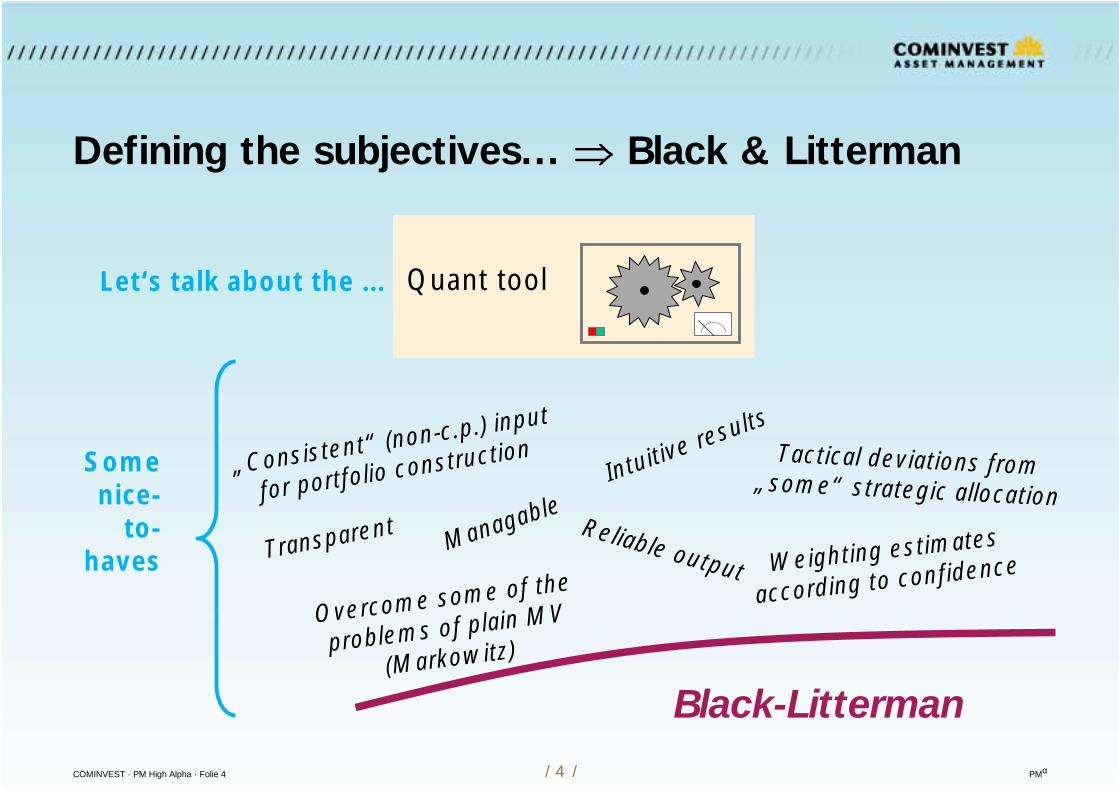
Defining the subjectives... Black & Litterman
Let‘s talk about the ... Quant tool
„Consistent“ (non-c.p.) input
for portfolio construction
Overcome some of the
problems of plain MV
(Markowitz)
Tactical deviations from„some“ strategic allocation
TransparentWeighting estimates
according to confidence
Black-Litterman
ManagableReliable output
Intuitive results
Somenice-
to-haves

COMINVEST · PM High Alpha · Folie 5 / 5 / PMα
Topics to be discussed...
Markowitz - Efficient Portfolios
Classical Markowitz - the straight way
MV-optimized portfolios
BL - the role within the investment process
BL - implementation
BL - example
COMINVEST · PM High Alpha · Folie 6 / 6 / PMα
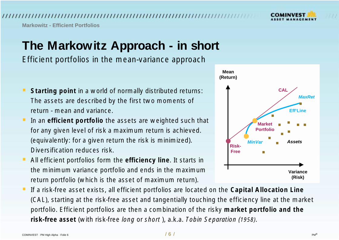
Starting point in a world of normally distributed returns:The assets are described by the first two moments ofreturn - mean and variance.
In an efficient portfolio the assets are weighted such thatfor any given level of risk a maximum return is achieved.(equivalently: for a given return the risk is minimized).Diversification reduces risk.
All efficient portfolios form the efficiency line. It starts inthe minimum variance portfolio and ends in the maximumreturn portfolio (which is the asset of maximum return).
If a risk-free asset exists, all efficient portfolios are located on the Capital Allocation Line(CAL), starting at the risk-free asset and tangentially touching the efficiency line at the marketportfolio. Efficient portfolios are then a combination of the risky market portfolio and therisk-free asset (with risk-free long or short ), a.k.a. Tobin Separation (1958).
The Markowitz Approach - in short
Markowitz - Efficient Portfolios
Efficient portfolios in the mean-variance approachMean
(Return)
Variance(Risk)
MinVar
MaxRet
MarketPortfolio
CAL
Eff‘Line
Risk-Free
Assets
COMINVEST · PM High Alpha · Folie 7 / 7 / PMα
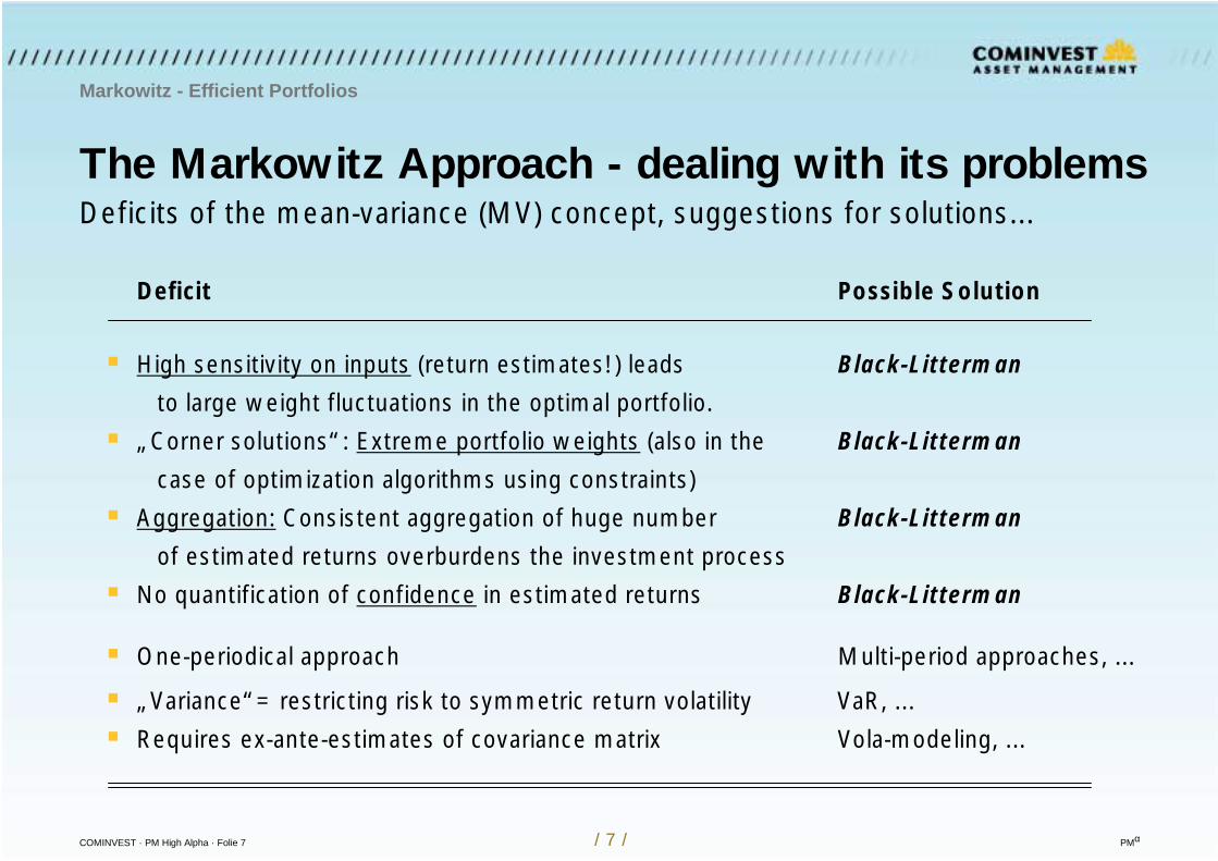
The Markowitz Approach - dealing with its problems
Deficit Possible Solution
High sensitivity on inputs (return estimates!) leads Black-Litterman
to large weight fluctuations in the optimal portfolio.
„Corner solutions“: Extreme portfolio weights (also in the Black-Litterman
case of optimization algorithms using constraints)
Aggregation: Consistent aggregation of huge number Black-Litterman
of estimated returns overburdens the investment process
No quantification of confidence in estimated returns Black-Litterman
One-periodical approach Multi-period approaches, ...
„Variance“= restricting risk to symmetric return volatility VaR, ...
Requires ex-ante-estimates of covariance matrix Vola-modeling, ...
Markowitz - Efficient Portfolios
Deficits of the mean-variance (MV) concept, suggestions for solutions...
COMINVEST · PM High Alpha · Folie 8 / 8 / PMα
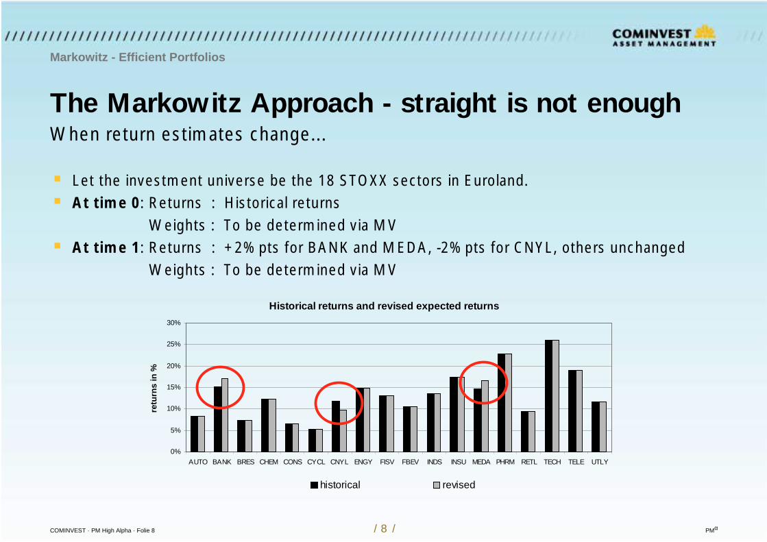
The Markowitz Approach - straight is not enough
Let the investment universe be the 18 STOXX sectors in Euroland. At time 0: Returns : Historical returns
Weights : To be determined via MV At time 1: Returns : +2%pts for BANK and MEDA, -2%pts for CNYL, others unchanged
Weights : To be determined via MV
Markowitz - Efficient Portfolios
When return estimates change...
Historical returns and revised expected returns
0%
5%
10%
15%
20%
25%
30%
AUTO BANK BRES CHEM CONS CYCL CNYL ENGY FISV FBEV INDS INSU MEDA PHRM RETL TECH TELE UTLY
retu
rns
in %
historical revised
COMINVEST · PM High Alpha · Folie 9 / 9 / PMα
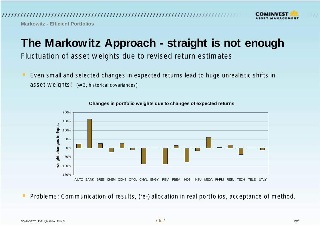
The Markowitz Approach - straight is not enough
Even small and selected changes in expected returns lead to huge unrealistic shifts inasset weights! (γ=3, historical covariances)
Problems: Communication of results, (re-) allocation in real portfolios, acceptance of method.
Markowitz - Efficient Portfolios
Fluctuation of asset weights due to revised return estimates
Changes in portfolio weights due to changes of expected returns
-150%
-100%
-50%
0%
50%
100%
150%
200%
AUTO BANK BRES CHEM CONS CYCL CNYL ENGY FISV FBEV INDS INSU MEDA PHRM RETL TECH TELE UTLY
wei
ght c
hang
es in
%pt
s.
COMINVEST · PM High Alpha · Folie 10 / 10 / PMα
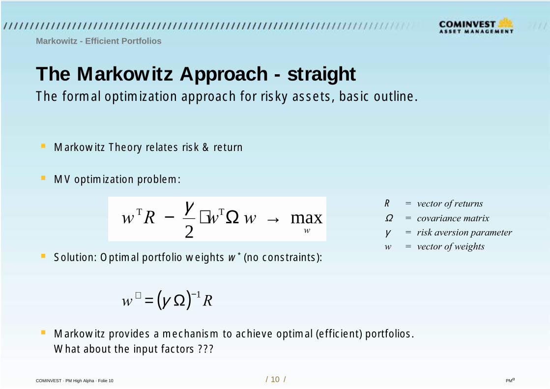
Markowitz Theory relates risk & return
MV optimization problem:
Solution: Optimal portfolio weights w* (no constraints):
Markowitz provides a mechanism to achieve optimal (efficient) portfolios.What about the input factors ???
The Markowitz Approach - straight
Markowitz - Efficient Portfolios
The formal optimization approach for risky assets, basic outline.
max 2
TT
wwwRw →Ω⋅− γ
( ) Rw 1 −∗ Ω= γ
R = vector of returnsΩ = covariance matrixγ = risk aversion parameterw = vector of weights
COMINVEST · PM High Alpha · Folie 11 / 11 / PMα
Extending the Markowitz Approach
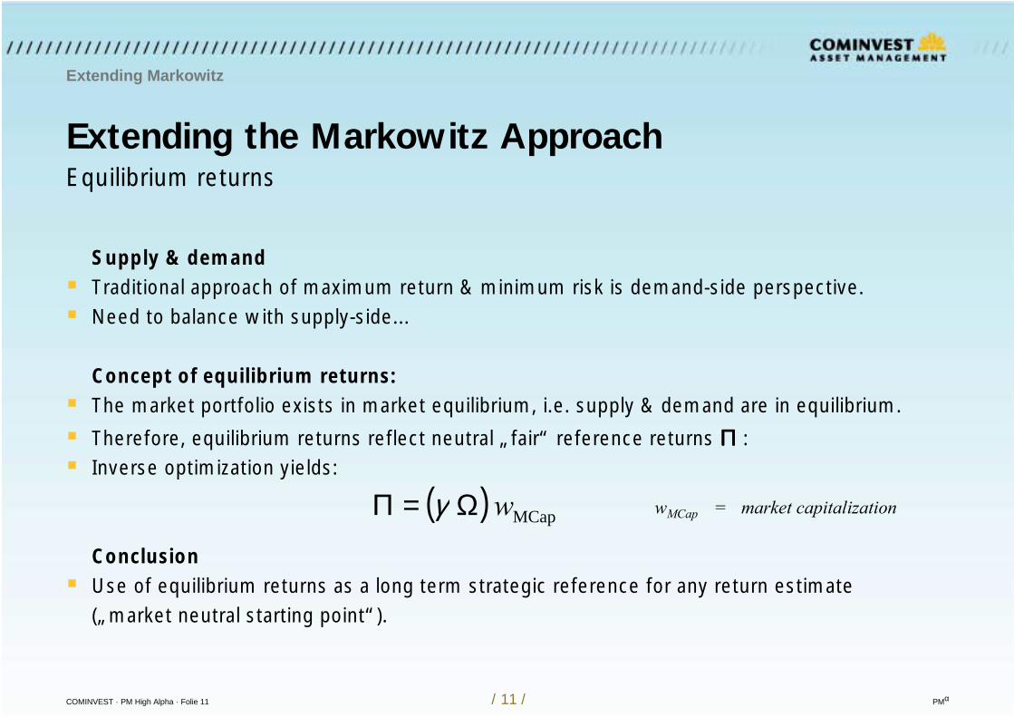
Supply & demand Traditional approach of maximum return & minimum risk is demand-side perspective. Need to balance with supply-side...
Concept of equilibrium returns: The market portfolio exists in market equilibrium, i.e. supply & demand are in equilibrium.
Therefore, equilibrium returns reflect neutral „fair“ reference returns Π Π Π Π : Inverse optimization yields:
Conclusion Use of equilibrium returns as a long term strategic reference for any return estimate
(„market neutral starting point“).
Extending Markowitz
Equilibrium returns
( ) MCap wΩ=Π γ wMCap = market capitalization
COMINVEST · PM High Alpha · Folie 12 / 12 / PMα
Extending the Markowitz Approach
Extending Markowitz
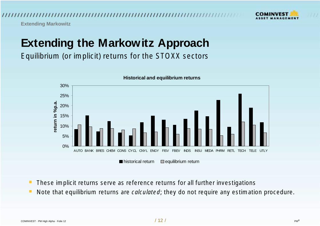
Equilibrium (or implicit) returns for the STOXX sectors
These implicit returns serve as reference returns for all further investigations Note that equilibrium returns are calculated; they do not require any estimation procedure.
Historical and equilibrium returns
0%
5%
10%
15%
20%
25%
30%
AUTO BANK BRES CHEM CONS CYCL CNYL ENGY FISV FBEV INDS INSU MEDA PHRM RETL TECH TELE UTLY
retu
rn in
%p.
a.
historical return equilibrium return
COMINVEST · PM High Alpha · Folie 13 / 13 / PMα
Research
Black-Litterman Approach - basic outline
Black-Litterman Process
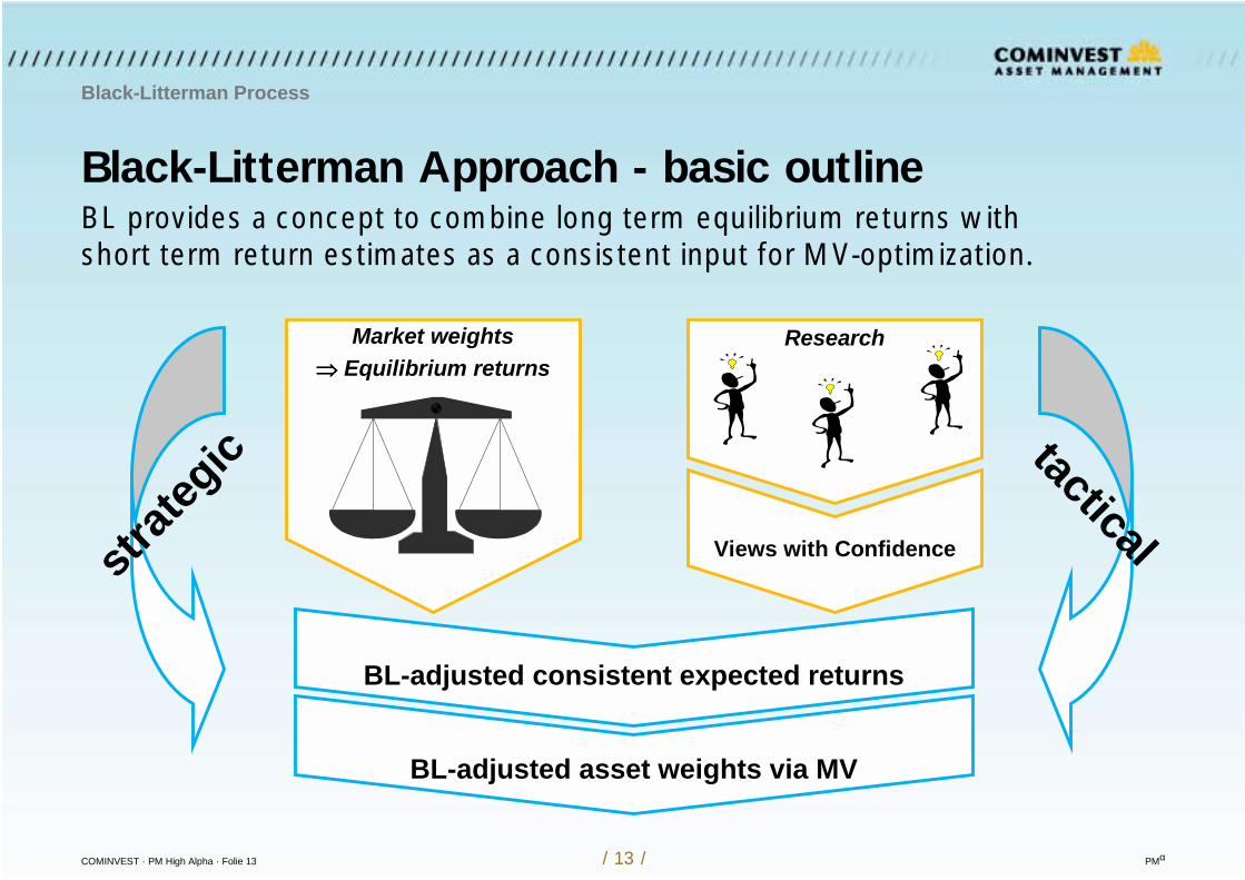
BL provides a concept to combine long term equilibrium returns with short term return estimates as a consistent input for MV-optimization.
Views with Confidencestrate
gic tactical
Market weights Equilibrium returns
BL-adjusted consistent expected returns
BL-adjusted asset weights via MV
COMINVEST · PM High Alpha · Folie 14 / 14 / PMα
Black-Litterman Approach - going math
BL Optimization Problem
Optimization s.t. contraints
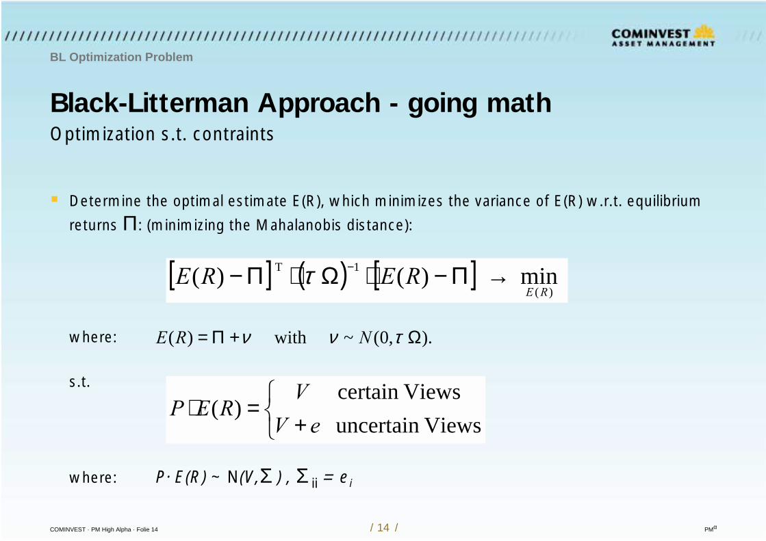
Determine the optimal estimate E(R), which minimizes the variance of E(R) w.r.t. equilibrium
returns Π: (minimizing the Mahalanobis distance):
where:
s.t.
where: P· E(R) ~ N(V,Σ ) , Σ ii = ei
+=⋅
Viewsuncertain Viewscertain
)(eV
VREP
[ ] ( ) [ ] min )( )()(
1T
RERERE →Π−⋅Ω⋅Π− −τ
). ,0(~ with )( Ω+Π= τνν NRE
COMINVEST · PM High Alpha · Folie 15 / 15 / PMα
Black-Litterman Approach - the formulas
BL Optimization Problem
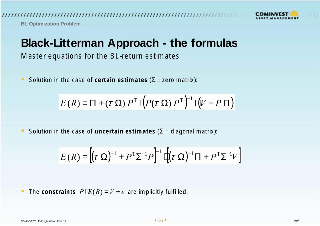
Master equations for the BL-return estimates
Solution in the case of certain estimates (Σ ≡ zero matrix):
Solution in the case of uncertain estimates (Σ = diagonal matrix):
The constraints are implicitly fulfilled.
( ) ( )Π−⋅Ω⋅Ω+Π= − ) ( ) ()( 1TT PVPPPRE ττ
( )[ ] ( )[ ]VPPPRE 1T111T1 )( −−−−− Σ+ΠΩ⋅Σ+Ω= ττ
eVREP +=⋅ )(
COMINVEST · PM High Alpha · Folie 16 / 16 / PMα
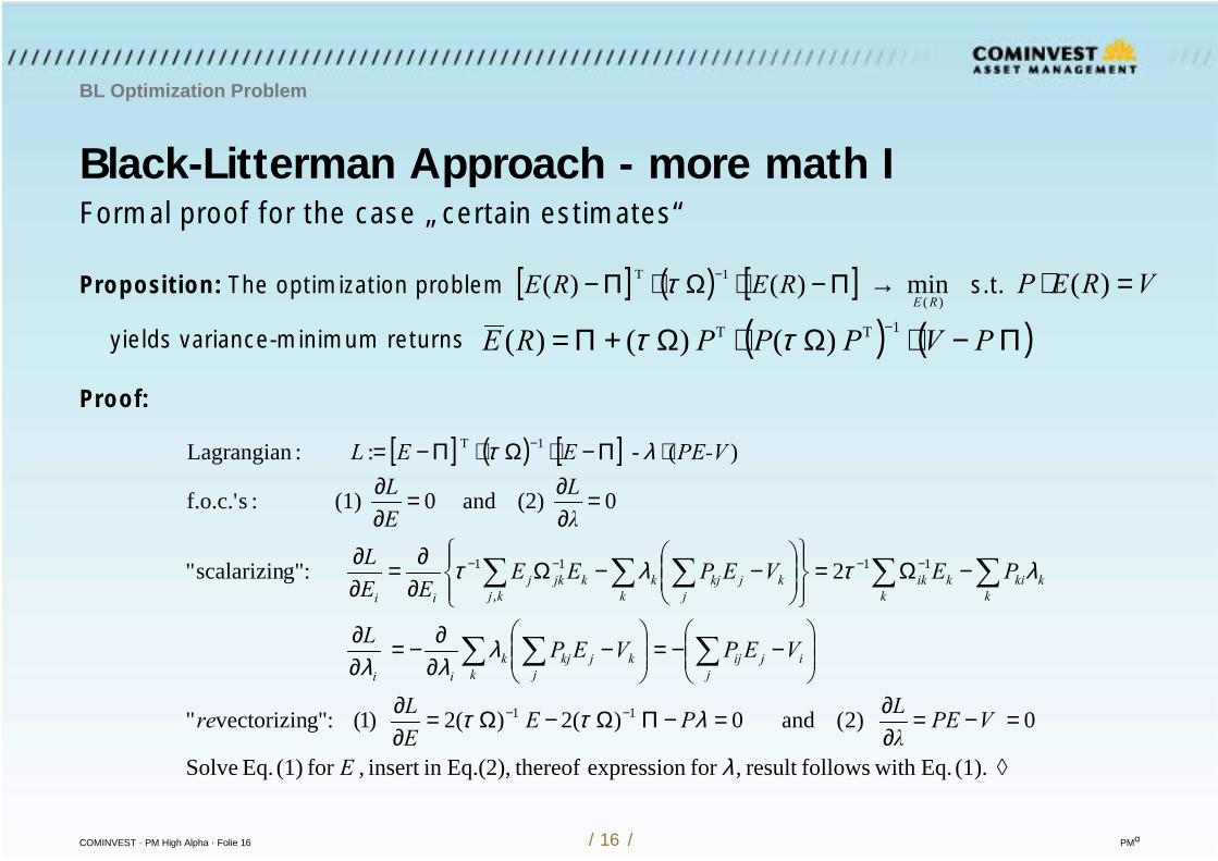
Black-Litterman Approach - more math I
BL Optimization Problem
Formal proof for the case „certain estimates“
Proposition: The optimization problem s.t.
yields variance-minimum returns
Proof:
[ ] ( ) [ ] min )( )()(
1T
RERERE →Π−⋅Ω⋅Π− −τ VREP =⋅ )(
[ ] ( ) [ ]
=−=∂∂=−ΠΩ−Ω=
∂∂
−−=
−
∂∂−=
∂∂
−Ω=
−−Ω
∂∂=
∂∂
=∂∂=
∂∂
⋅Π−⋅Ω⋅Π−=
−−
−−−−
−
(1). Eq. with followsresult ,for expression thereofEq.(2),in insert , for (1) Eq. Solve
0 )2( and 0 ) (2 ) (2 )1( :"gvectorizin"
2 :g"scalarizin"
0 (2) and 0 (1) :sf.o.c.'
)( - : :Lagrangian
11
11
,
11
1T
λ
λττ
λλλ
λτλτ
λτ
E
VPEλLPE
EL re
VEPVEPL
PEVEPEEEE
LλL
EL
PE-VEEL
jijij
jkjkj
kk
ii
kkkik
kik
k jkjkjk
kjkjkj
ii
( ) ( )Π−⋅Ω⋅Ω+Π= − ) ( ) ()( 1TT PVPPPRE ττ
COMINVEST · PM High Alpha · Folie 17 / 17 / PMα
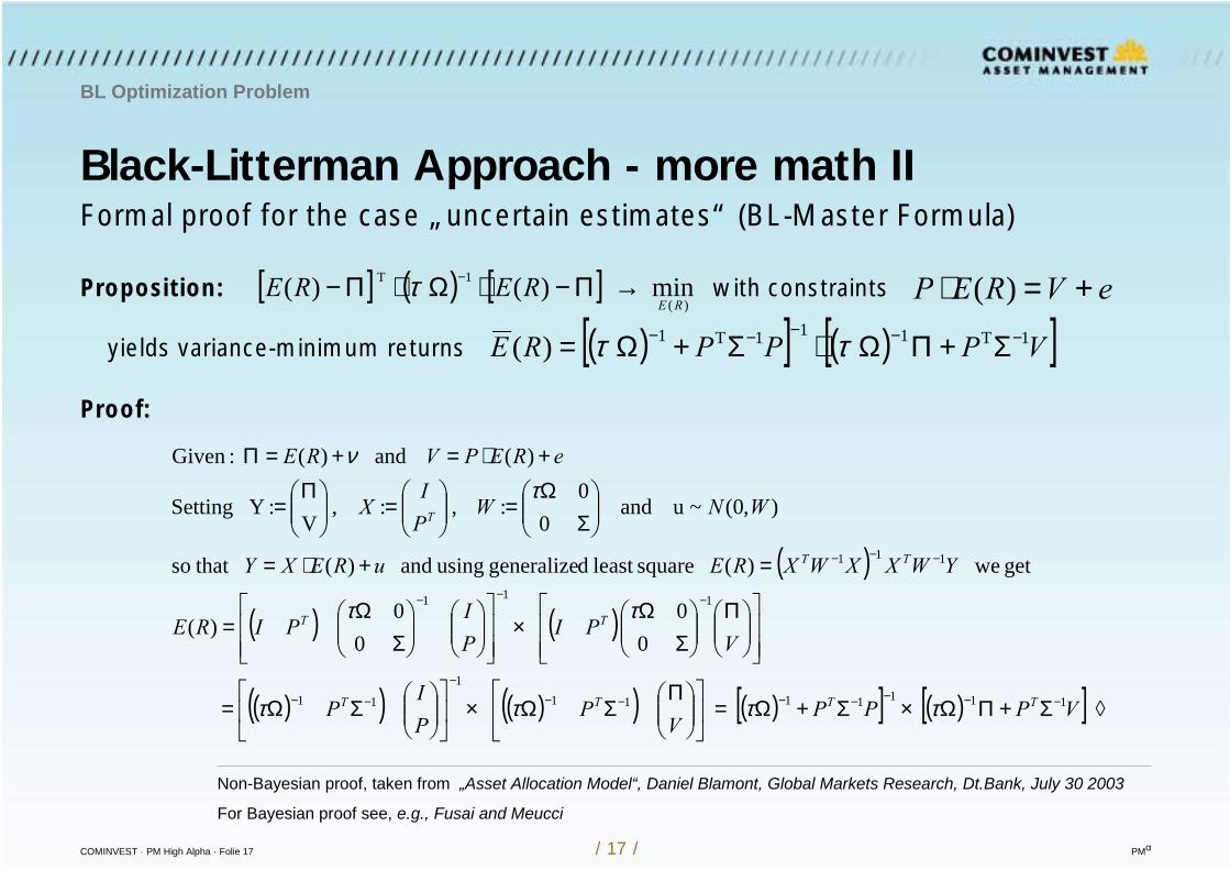
Black-Litterman Approach - more math II
BL Optimization Problem
Formal proof for the case „uncertain estimates“ (BL-Master Formula)
Proposition: with constraints
yields variance-minimum returns
Proof:
[ ] ( ) [ ] min )( )()(
1T
RERERE →Π−⋅Ω⋅Π− −τ eVREP +=⋅ )(
( )
( ) ( )
( )( ) ( )( ) ( )[ ] ( )[ ] Σ+ΠΩ×Σ+Ω=
ΠΣΩ×
ΣΩ=
Π
ΣΩ
×
ΣΩ
=
=+⋅=
ΣΩ
=
=
Π=
+⋅=+=Π
−−−−−−−−
−−
−−−
−−−
00
0
0)(
get we)( squareleast dgeneralize using and )( that so
),0(~u and 0
0: , : ,
V:Y Setting
)( and )( :Given
11111111
11
111
111
VPPPV
PPI
P
VPI
PI
PIRE
YWXXWXREuREXY
WNWPI
X
eREPVRE
TTTT
TT
TT
T
ττττ
ττ
τν
( )[ ] ( )[ ]VPPPRE 1T111T1 )( −−−−− Σ+ΠΩ⋅Σ+Ω= ττ
Non-Bayesian proof, taken from „Asset Allocation Model“, Daniel Blamont, Global Markets Research, Dt.Bank, July 30 2003
For Bayesian proof see, e.g., Fusai and Meucci
COMINVEST · PM High Alpha · Folie 18 / 18 / PMα
1I_
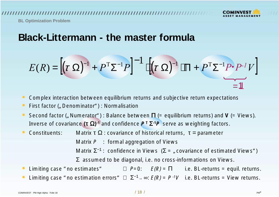
Black-Littermann - the master formula
BL Optimization Problem
Complex interaction between equilibrium returns and subjective return expectations First factor („Denominator“) : Normalisation
Second factor („Numerator“) : Balance between ΠΠΠΠ (= equilibrium returns) and V (= Views). Inverse of covariance (τ Ωτ Ωτ Ωτ Ω)-1 and confidence P T ΣΣΣΣ-1P serve as weighting factors.
Constituents: Matrix τ Ω : covariance of historical returns, τ = parameter
Matrix P : formal aggregation of Views
Matrix Σ−1 : confidence in Views (Σ = „covariance of estimated Views“)
Σ assumed to be diagonal, i.e. no cross-informations on Views.
Limiting case “no estimates“ ⇔ P=0: E(R) = Π i.e. BL-returns = equil. returns.
Limiting case “no estimation errors“ ⇔ Σ−1→ ∞: E(R) = P -1V i.e. BL-returns = View returns.
( )[ ] ( )[ ]VPPPRE 1
)( 1T1 1T1 −−−− Σ+Π⋅Ω⋅−
Σ+Ω= ττ
=
P·P-1
COMINVEST · PM High Alpha · Folie 19 / 19 / PMα
Black-Litterman Approach - remarks
BL Optimization Problem
Use of CAPM to determine equilibrium returns
Alternative to inverse optimization: Equilibrium returns ΠΕq from CAPM Additional input for CAPM: Risk-free rate rf , risk premium vs market (M), Beta coefficients Evaluation:
(fair return for asset i ) with
BL returns as a Bayesian a-posteriori estimator
Bayes Theorem (or “Law“ or “Rule“) states how to determine conditional expectations. Given an a-priori known distribution of a random variable. Adding new information leads to a revised conditional distribution, the so-called a-posteriori distribution (result of „learning“). BL-return estimates are a-posteriori (multivariate) normally distributed return expectations.
( ) 2, M
iMifMifEqi rrr
σσββ =−⋅+=Π
COMINVEST · PM High Alpha · Folie 20 / 20 / PMα
Black-Litterman Approach - γγγγ
Parameters in BL
Remark: Risk aversion parameter γ
How does risk change for an additional bp of return?
Suggestions:
Satchell & Scowcroft and Best & Grauer:
Let γ = (rM-rf) / σM2
where σM2 = wT Ω w , w = market cap.
Zimmermann et al.: σM=16.9% p.a. for STOXX-data (own calculation) Chose γ = 3, which corresponds to a risk premium of 8.6%.
Idzorek: (DJIA, USA): Risk premium=7.5%: γ = 2.25.
COMINVEST · PM High Alpha · Folie 21 / 21 / PMα
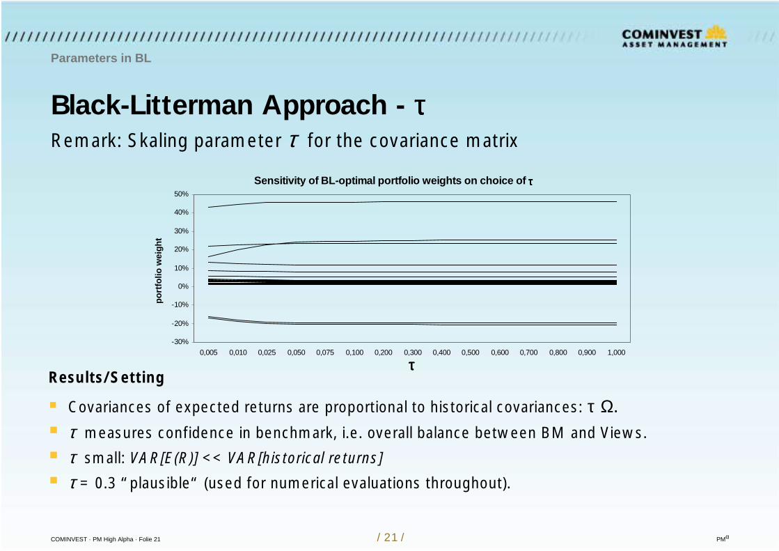
Black-Litterman Approach - ττττ
Parameters in BL
Remark: Skaling parameter τ for the covariance matrix
Results/Setting
Covariances of expected returns are proportional to historical covariances: τ Ω. τ measures confidence in benchmark, i.e. overall balance between BM and Views.
τ small: VAR[E(R)] << VAR[historical returns]
τ = 0.3 “plausible“ (used for numerical evaluations throughout).
Sensitivity of BL-optimal portfolio weights on choice of ττττ
-30%
-20%
-10%
0%
10%
20%
30%
40%
50%
0,005 0,010 0,025 0,050 0,075 0,100 0,200 0,300 0,400 0,500 0,600 0,700 0,800 0,900 1,000
ττττ
port
folio
wei
ght
COMINVEST · PM High Alpha · Folie 22 / 22 / PMα
Black-Litterman Approach - some real problems
Parameters in BL
Additional remarks on the recent remarks
Calibration problems with parameter τ (“plausible“, “adjusted to IR=1“, ... )
Calibration problems with parameter γ (“world wide risk aversion“, ... )
Calibration problems with expressing the degree of confidence (“1..3“, “0..100%“)
COMINVEST · PM High Alpha · Folie 23 / 23 / PMα
Black-Litterman Approach - Views
BL-Views
Implementing Views on expected returns deviating from equilibrium figures
Views Return estimates differing from the (strategic) equilibrium returns are
the essential input to the BL estimation process.
Specification of Views ... as absolute return expectations for individual assets
and / or ... as relative return expectations relating assets or aggregates of assets.
Formal constraint: #Views ≤ #Assets.
Confidence Each View has to be assigned the level of confidence for an interval of uncertainty.
Selective Views Views can be restricted to selected assets for which in-depth analysis is available.
COMINVEST · PM High Alpha · Folie 24 / 24 / PMα
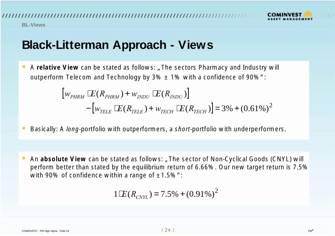
Black-Litterman Approach - Views
BL-Views
A relative View can be stated as follows: „The sectors Pharmacy and Industry willoutperform Telecom and Technology by 3% ± 1% with a confidence of 90%“:
Basically: A long-portfolio with outperformers, a short-portfolio with underperformers.
An absolute View can be stated as follows: „The sector of Non-Cyclical Goods (CNYL) willperform better than stated by the equilibrium return of 6.66%. Our new target return is 7.5%with 90% of confidence within a range of ±1.5%“:
[ ][ ] 2%)61.0(%3)()(
)()(
+=⋅+⋅−
⋅+⋅
TECHTECHTELETELE
INDUINDUPHRMPHRM
REwREw
REwREw
2%)91.0(%5.7)(1 +=⋅ CNYLRE
COMINVEST · PM High Alpha · Folie 25 / 25 / PMα
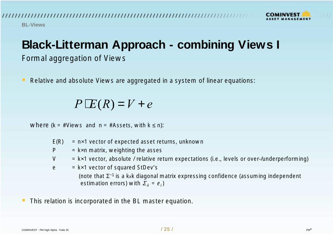
Black-Litterman Approach - combining Views I
BL-Views
Formal aggregation of Views
Relative and absolute Views are aggregated in a system of linear equations:
where (k = #Views and n = #Assets, with k ≤ n):
E(R) = n×1 vector of expected asset returns, unknownP = k×n matrix, weighting the assesV = k×1 vector, absolute / relative return expectations (i.e., levels or over-/underperforming)e = k×1 vector of squared StDev‘s
(note that Σ−1 is a kxk diagonal matrix expressing confidence (assuming independent estimation errors) with Σ ii = ei )
This relation is incorporated in the BL master equation.
eVREP +=⋅ )(
COMINVEST · PM High Alpha · Folie 26 / 26 / PMα
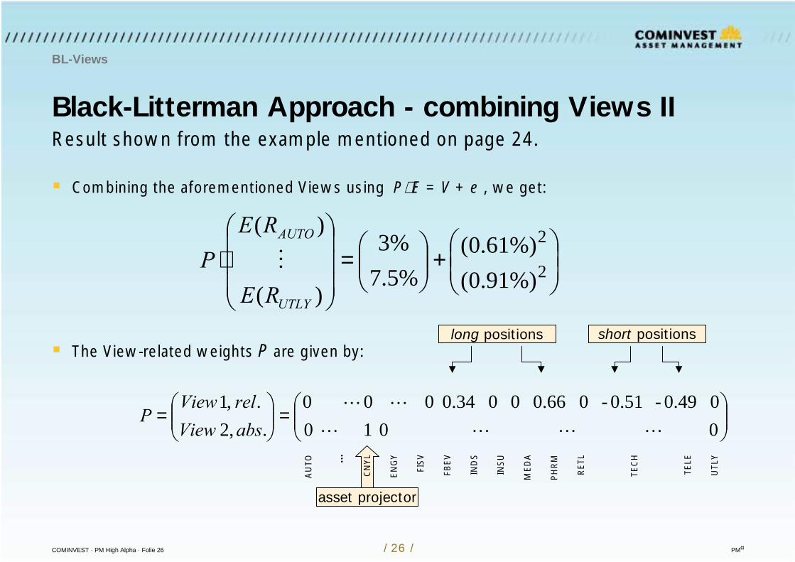
Black-Litterman Approach - combining Views II
BL-Views
Combining the aforementioned Views using P⋅ E = V + e , we get:
The View-related weights P are given by:
+
=
⋅ 2
2
%)91.0(%)61.0(
%5.7%3
)(
)(
UTLY
AUTO
RE
REP
=
=
0 0 1 00 0.49- 0.51- 0 0.66 0 0 0.34 0 0 0
.,2 . ,1
absViewrelView
P
long positions short positions
asset projector
AU
TO ...
CN
YL
EN
GY
FIS
V
FBE
V
IND
S
INS
U
ME
DA
PH
RM
RE
TL
TEC
H
TELE
UTL
Y
Result shown from the example mentioned on page 24.
COMINVEST · PM High Alpha · Folie 27 / 27 / PMα
Black-Litterman Approach - confidence
BL-Views
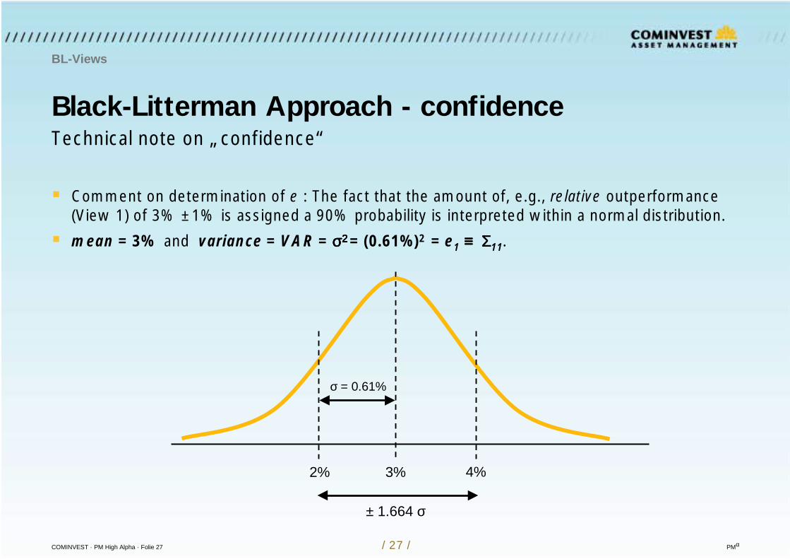
Technical note on „confidence“
Comment on determination of e : The fact that the amount of, e.g., relative outperformance(View 1) of 3% ±1% is assigned a 90% probability is interpreted within a normal distribution.
mean = 3% and variance = VAR = σσσσ2 2 2 2 = (0.61%)2 = e1 ≡≡≡≡ ΣΣΣΣ11.
σ = 0.61%
2% 3% 4%
± 1.664 σ
COMINVEST · PM High Alpha · Folie 28 / 28 / PMα
Black-Litterman Approach - example in detail
Example: DJ STOXX
„Sector allocation, Dow Jones STOXX“
Example follows the lines of „Einsatz des Black-Litterman-Verfahrens in der Asset Allocation“, H.Zimmermann et al. publ. in „Handbuch Asset Allocation“ (Editors: Dichtl, Schlenger u. Kleeberg, publ. by Uhlenbruch-Verlag, 2002).
Notation, scenarios and data therein have been used, some data were missing.
Missing data - volatilities and covariances - had to be calculated from scratch, thus causingsome deviations in the numerical results between this presentation and cited literature.Nevertheless, all relevant results are reproduced.
All calculations can be (have been) implemented and performed in Excel (TM).
COMINVEST · PM High Alpha · Folie 29 / 29 / PMα
Black-Litterman Approach - the data
Example: DJ STOXX
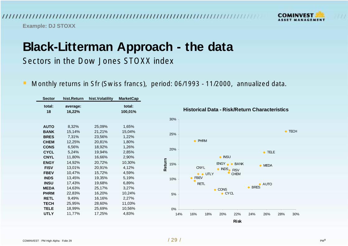
Sectors in the Dow Jones STOXX index
Monthly returns in Sfr (Swiss francs), period: 06/1993 - 11/2000, annualized data.
Historical Data - Risk/Return Characteristics
UTLY
TELE
RETL
PHRM
MEDA
INSU
INDS
FBEV
FISV
ENGYCNYL
CYCLCONS
CHEM
BRES
BANK
AUTO
TECH
0%
5%
10%
15%
20%
25%
30%
14% 16% 18% 20% 22% 24% 26% 28% 30%
Risk
Ret
urn
Sector hist.Return hist.Volatility MarketCap
total: average: total:18 16,22% 100,01%
AUTO 8,32% 25,09% 1,65%BANK 15,14% 21,21% 15,04%BRES 7,31% 23,56% 1,22%CHEM 12,25% 20,81% 1,80%CONS 6,56% 18,92% 1,26%CYCL 5,24% 19,94% 2,85%CNYL 11,80% 16,66% 2,90%ENGY 14,92% 20,72% 10,30%FISV 13,01% 20,91% 4,12%FBEV 10,47% 15,72% 4,59%INDS 13,45% 19,35% 5,19%INSU 17,43% 19,68% 6,89%MEDA 14,63% 25,17% 3,27%PHRM 22,83% 16,20% 10,24%RETL 9,49% 16,16% 2,27%TECH 25,95% 28,60% 11,03%TELE 18,99% 25,69% 10,56%UTLY 11,77% 17,25% 4,83%
COMINVEST · PM High Alpha · Folie 30 / 30 / PMα
Black-Litterman Approach - the correlations
Example: DJ STOXX
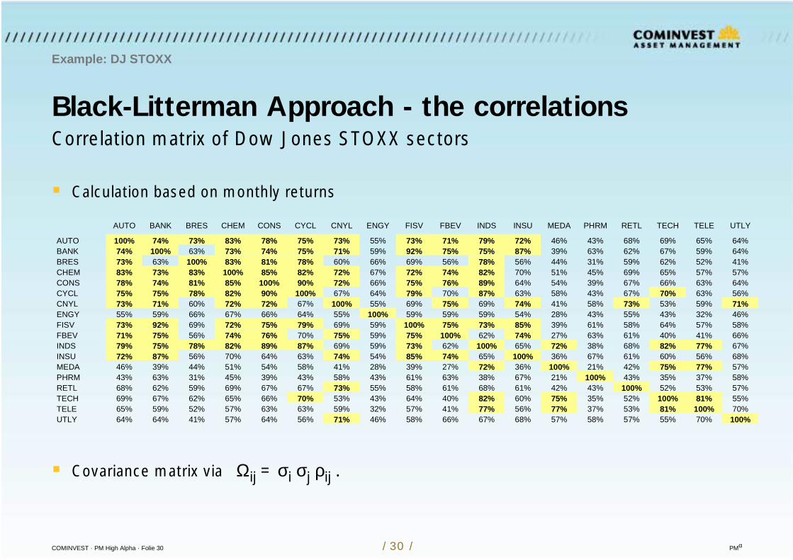
Correlation matrix of Dow Jones STOXX sectors
AUTO BANK BRES CHEM CONS CYCL CNYL ENGY FISV FBEV INDS INSU MEDA PHRM RETL TECH TELE UTLY
AUTO 100% 74% 73% 83% 78% 75% 73% 55% 73% 71% 79% 72% 46% 43% 68% 69% 65% 64%BANK 74% 100% 63% 73% 74% 75% 71% 59% 92% 75% 75% 87% 39% 63% 62% 67% 59% 64%BRES 73% 63% 100% 83% 81% 78% 60% 66% 69% 56% 78% 56% 44% 31% 59% 62% 52% 41%CHEM 83% 73% 83% 100% 85% 82% 72% 67% 72% 74% 82% 70% 51% 45% 69% 65% 57% 57%CONS 78% 74% 81% 85% 100% 90% 72% 66% 75% 76% 89% 64% 54% 39% 67% 66% 63% 64%CYCL 75% 75% 78% 82% 90% 100% 67% 64% 79% 70% 87% 63% 58% 43% 67% 70% 63% 56%CNYL 73% 71% 60% 72% 72% 67% 100% 55% 69% 75% 69% 74% 41% 58% 73% 53% 59% 71%ENGY 55% 59% 66% 67% 66% 64% 55% 100% 59% 59% 59% 54% 28% 43% 55% 43% 32% 46%FISV 73% 92% 69% 72% 75% 79% 69% 59% 100% 75% 73% 85% 39% 61% 58% 64% 57% 58%FBEV 71% 75% 56% 74% 76% 70% 75% 59% 75% 100% 62% 74% 27% 63% 61% 40% 41% 66%INDS 79% 75% 78% 82% 89% 87% 69% 59% 73% 62% 100% 65% 72% 38% 68% 82% 77% 67%INSU 72% 87% 56% 70% 64% 63% 74% 54% 85% 74% 65% 100% 36% 67% 61% 60% 56% 68%MEDA 46% 39% 44% 51% 54% 58% 41% 28% 39% 27% 72% 36% 100% 21% 42% 75% 77% 57%PHRM 43% 63% 31% 45% 39% 43% 58% 43% 61% 63% 38% 67% 21% 100% 43% 35% 37% 58%RETL 68% 62% 59% 69% 67% 67% 73% 55% 58% 61% 68% 61% 42% 43% 100% 52% 53% 57%TECH 69% 67% 62% 65% 66% 70% 53% 43% 64% 40% 82% 60% 75% 35% 52% 100% 81% 55%TELE 65% 59% 52% 57% 63% 63% 59% 32% 57% 41% 77% 56% 77% 37% 53% 81% 100% 70%UTLY 64% 64% 41% 57% 64% 56% 71% 46% 58% 66% 67% 68% 57% 58% 57% 55% 70% 100%
Calculation based on monthly returns
Covariance matrix via Ωij = σi σj ρij .
COMINVEST · PM High Alpha · Folie 31 / 31 / PMα
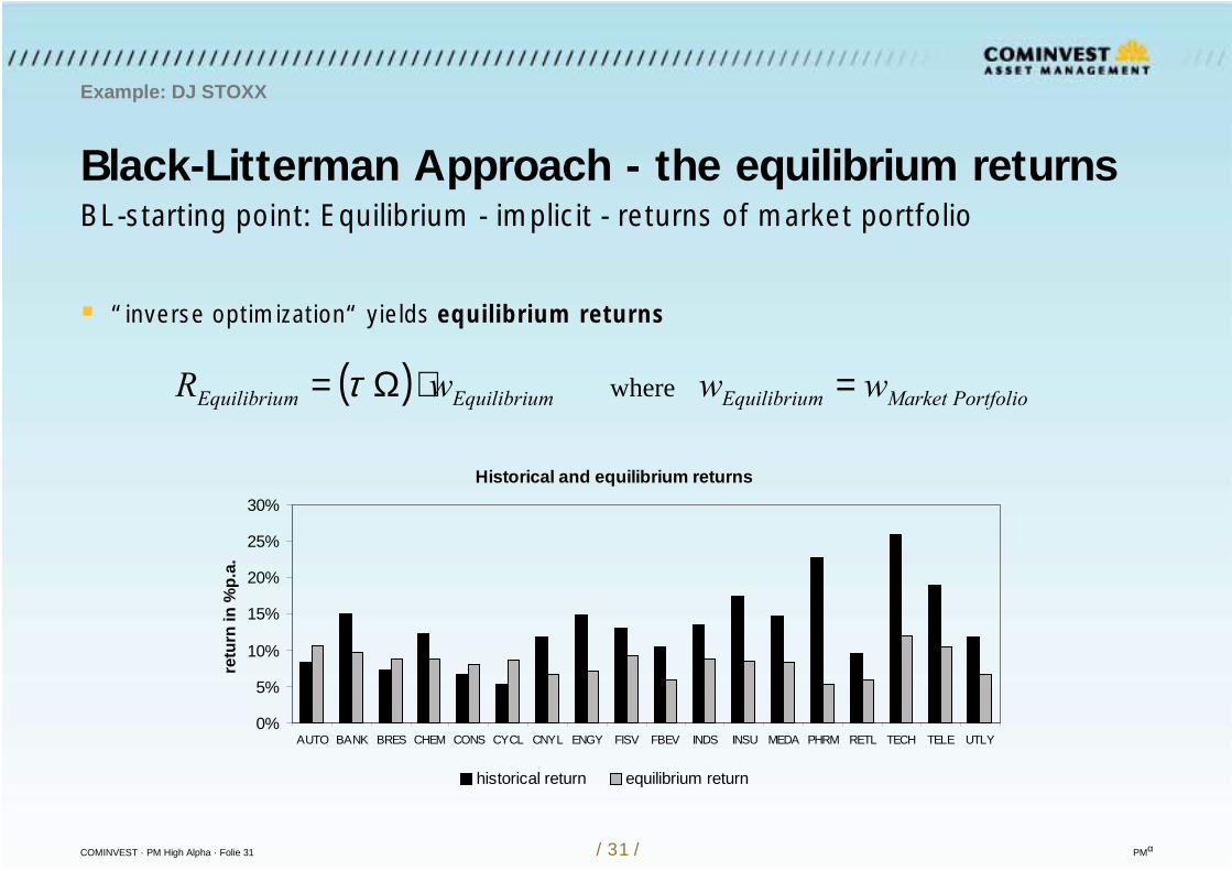
Black-Litterman Approach - the equilibrium returns
Example: DJ STOXX
BL-starting point: Equilibrium - implicit - returns of market portfolio
“inverse optimization“ yields equilibrium returns
( ) PortfolioMarketmEquilibriumEquilibriumEquilibriu wwwR where =⋅Ω= τ
Historical and equilibrium returns
0%
5%
10%
15%
20%
25%
30%
AUTO BANK BRES CHEM CONS CYCL CNYL ENGY FISV FBEV INDS INSU MEDA PHRM RETL TECH TELE UTLY
retu
rn in
%p.
a.
historical return equilibrium return
COMINVEST · PM High Alpha · Folie 32 / 32 / PMα
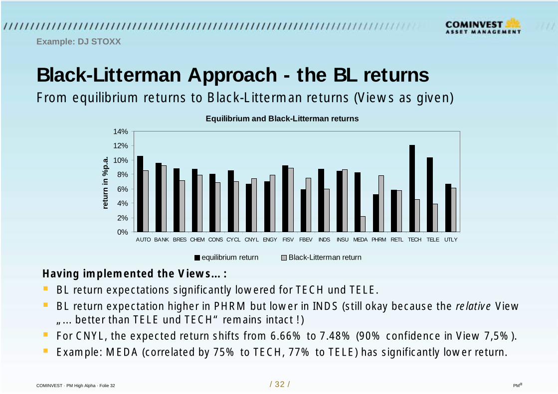
Black-Litterman Approach - the BL returns
Example: DJ STOXX
From equilibrium returns to Black-Litterman returns (Views as given)
Having implemented the Views... : BL return expectations significantly lowered for TECH und TELE. BL return expectation higher in PHRM but lower in INDS (still okay because the relative View
„... better than TELE und TECH“ remains intact !) For CNYL, the expected return shifts from 6.66% to 7.48% (90% confidence in View 7,5%). Example: MEDA (correlated by 75% to TECH, 77% to TELE) has significantly lower return.
Equilibrium and Black-Litterman returns
0%
2%
4%
6%
8%
10%
12%
14%
AUTO BANK BRES CHEM CONS CYCL CNYL ENGY FISV FBEV INDS INSU MEDA PHRM RETL TECH TELE UTLY
retu
rn in
%p.
a.
equilibrium return Black-Litterman return
COMINVEST · PM High Alpha · Folie 33 / 33 / PMα
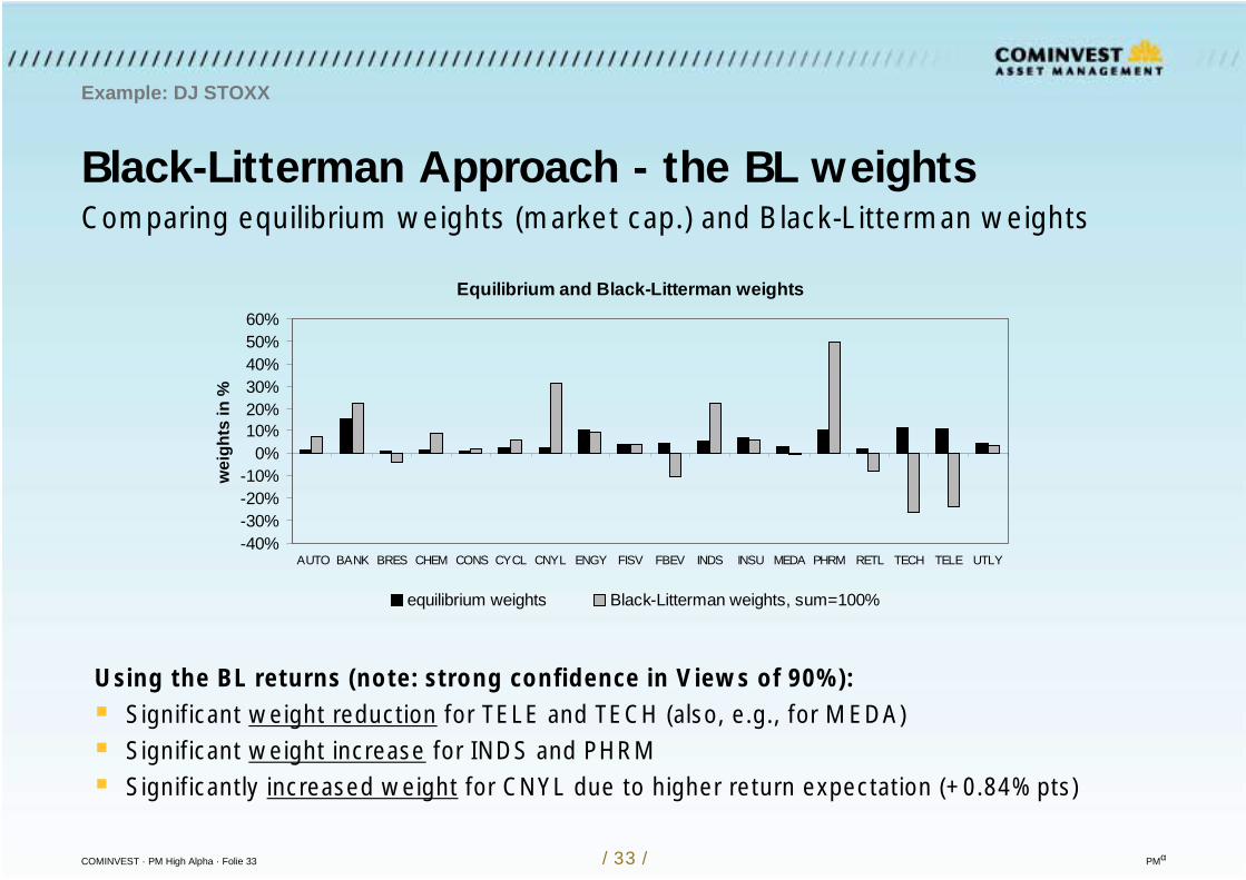
Black-Litterman Approach - the BL weights
Example: DJ STOXX
Comparing equilibrium weights (market cap.) and Black-Litterman weights
Using the BL returns (note: strong confidence in Views of 90%): Significant weight reduction for TELE and TECH (also, e.g., for MEDA) Significant weight increase for INDS and PHRM Significantly increased weight for CNYL due to higher return expectation (+0.84%pts)
Equilibrium and Black-Litterman weights
-40%-30%-20%-10%
0%10%20%30%40%50%60%
AUTO BANK BRES CHEM CONS CYCL CNYL ENGY FISV FBEV INDS INSU MEDA PHRM RETL TECH TELE UTLY
wei
ghts
in %
equilibrium weights Black-Litterman weights, sum=100%
COMINVEST · PM High Alpha · Folie 34 / 34 / PMα
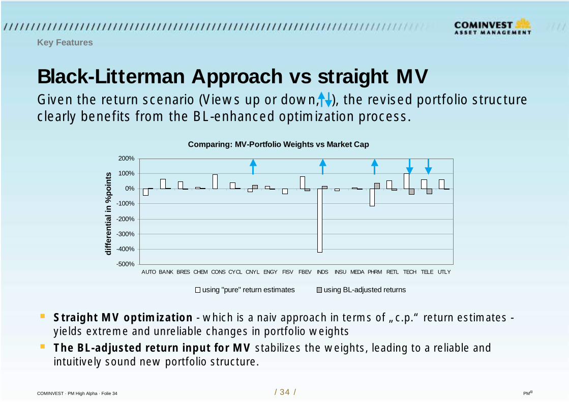
Comparing: MV-Portfolio Weights vs Market Cap
-500%
-400%
-300%
-200%
-100%
0%
100%
200%
AUTO BANK BRES CHEM CONS CYCL CNYL ENGY FISV FBEV INDS INSU MEDA PHRM RETL TECH TELE UTLY
diffe
rent
ial i
n %
poin
ts
using "pure" return estimates using BL-adjusted returns
Black-Litterman Approach vs straight MV
Key Features
Given the return scenario (Views up or down, ), the revised portfolio structureclearly benefits from the BL-enhanced optimization process.
Straight MV optimization - which is a naiv approach in terms of „c.p.“ return estimates -yields extreme and unreliable changes in portfolio weights
The BL-adjusted return input for MV stabilizes the weights, leading to a reliable andintuitively sound new portfolio structure.
COMINVEST · PM High Alpha · Folie 35 / 35 / PMα
Black-Litterman Approach - constraints I
Example: DJ STOXX
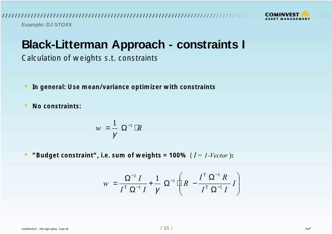
Calculation of weights s.t. constraints
In general: Use mean/variance optimizer with constraints
No constraints:
“Budget constraint“, i.e. sum of weights = 100% ( I = 1-Vector ):
Rw ⋅Ω= −1 1γ
ΩΩ
−⋅Ω+Ω
Ω= −
−−
−
−
IIIRI
RII
Iw
1
1T
1T1
1T
1
γ
COMINVEST · PM High Alpha · Folie 36 / 36 / PMα
Black-Litterman Approach - constraints II
Example: DJ STOXX
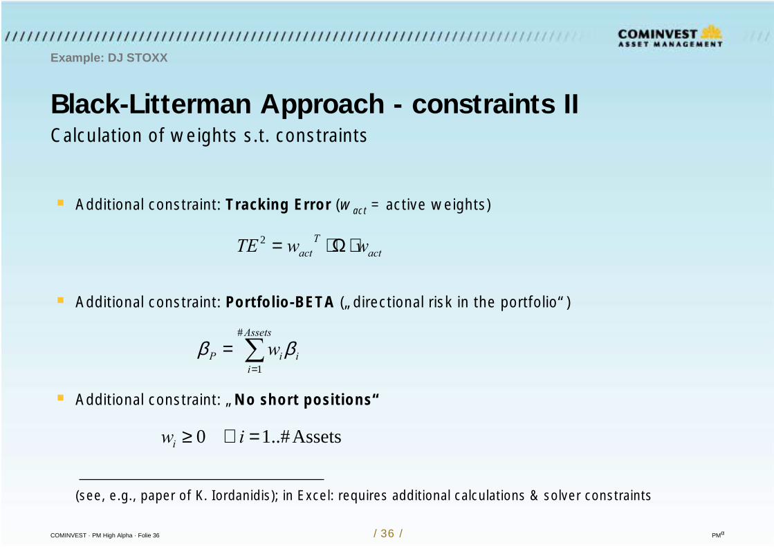
Calculation of weights s.t. constraints
Additional constraint: Tracking Error (wact = active weights)
Additional constraint: Portfolio-BETA („directional risk in the portfolio“)
Additional constraint: „No short positions“
(see, e.g., paper of K. Iordanidis); in Excel: requires additional calculations & solver constraints
actT
act wwTE ⋅Ω⋅=2
=
=Assets
iiiP w
#
1ββ
Assets..#1 0 =∀≥ iwi
COMINVEST · PM High Alpha · Folie 37 / 37 / PMα
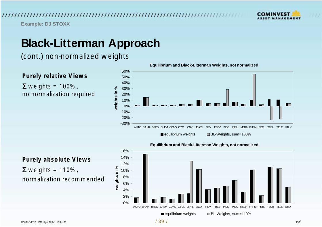
The sum of portfolio weights has to add up to 100%.
Purely absolute Views are translated into independent long and short portfolios, thus causingportfolio weights to deviate from 100%. Therefore, normalization of weights is recommended.
Purely relative Views are translated into weight-balanced long and short portfolios, so thatportfolio weights still sum up to 100%.
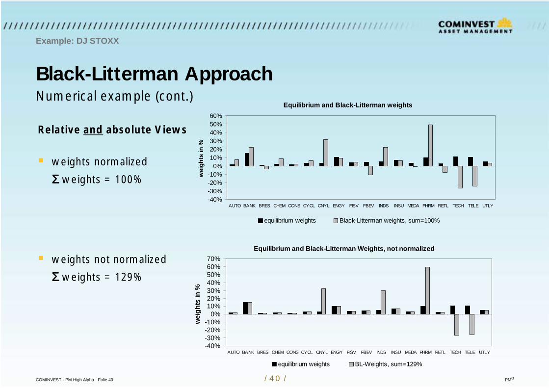
The use of absolute and relative Views again leads to portfolio weights deviating from 100%Therefore, again, normalization of weights is recommended.
The normalization to 100% has to be included in the optimization process as a constraint.
Note that - unfortunately - the use of constraints is contra-intuitive for BL-adjusted allocations.
Black-Litterman Approach - weights
Example: DJ STOXX
Remark on treating weights w.r.t. absolute / relative Views
COMINVEST · PM High Alpha · Folie 38 / 38 / PMα
Black-Litterman Approach
Example: DJ STOXX
Numerical example on treating weights w.r.t. absolute / relative Views
The example is based on the View scenario given on slide 24.
Purely absolute View: Weights add up to 110%, with all weights unchanged except for theasset (sector) CNYL under view (weight increases by 10%pts.).Normalization to 100% leads to weight changes in all positions - as it should be!(Note: Lowering the expected return of CNYL to, e.g., 5,5% yields a total portfolio weight of only 86%.Again, weight normalization is recommended, spreading for the -14%pts across all weights.)
Purely relative Views: Weights add up to 100%, with the weights of the viewed assets justoffsetting the long and short positions.
Absolute and relative Views: Weights add up to 129%, with long and short positions for theviewed assets as intuitively expected and the unviewed assets‘ weights remaining unchanged.Normalization to 100% consequently leads to weight changes in all positions - as it should be!
COMINVEST · PM High Alpha · Folie 39 / 39 / PMα
Black-Litterman Approach
Example: DJ STOXX
(cont.) non-normalized weightsEquilibrium and Black-Litterman Weights, not normalized
-30%-20%-10%
0%10%20%30%40%50%60%
AUTO BANK BRES CHEM CONS CYCL CNYL ENGY FISV FBEV INDS INSU MEDA PHRM RETL TECH TELE UTLY
wei
ghts
in %
equilibrium weights BL-Weights, sum=100%
Purely relative Views
ΣΣΣΣ weights = 100%, no normalization required
Purely absolute Views
ΣΣΣΣ weights = 110%, normalization recommended
Equilibrium and Black-Litterman Weights, not normalized
0%2%4%6%8%
10%12%14%16%
AUTO BANK BRES CHEM CONS CYCL CNYL ENGY FISV FBEV INDS INSU MEDA PHRM RETL TECH TELE UTLY
wei
ghts
in %
equilibrium weights BL-Weights, sum=110%
COMINVEST · PM High Alpha · Folie 40 / 40 / PMα
Black-Litterman Approach
Example: DJ STOXX
Numerical example (cont.)
Relative and absolute Views
weights normalized
ΣΣΣΣ weights = 100%
weights not normalized
ΣΣΣΣ weights = 129%
Equilibrium and Black-Litterman Weights, not normalized
-40%-30%-20%-10%
0%10%20%30%40%50%60%70%
AUTO BANK BRES CHEM CONS CYCL CNYL ENGY FISV FBEV INDS INSU MEDA PHRM RETL TECH TELE UTLY
wei
ghts
in %
equilibrium weights BL-Weights, sum=129%
Equilibrium and Black-Litterman weights
-40%-30%-20%-10%
0%10%20%30%40%50%60%
AUTO BANK BRES CHEM CONS CYCL CNYL ENGY FISV FBEV INDS INSU MEDA PHRM RETL TECH TELE UTLYw
eigh
ts in
%
equilibrium weights Black-Litterman weights, sum=100%
COMINVEST · PM High Alpha · Folie 41 / 41 / PMα
Black-Litterman Approach - confidence and CNYL
Example: DJ STOXX
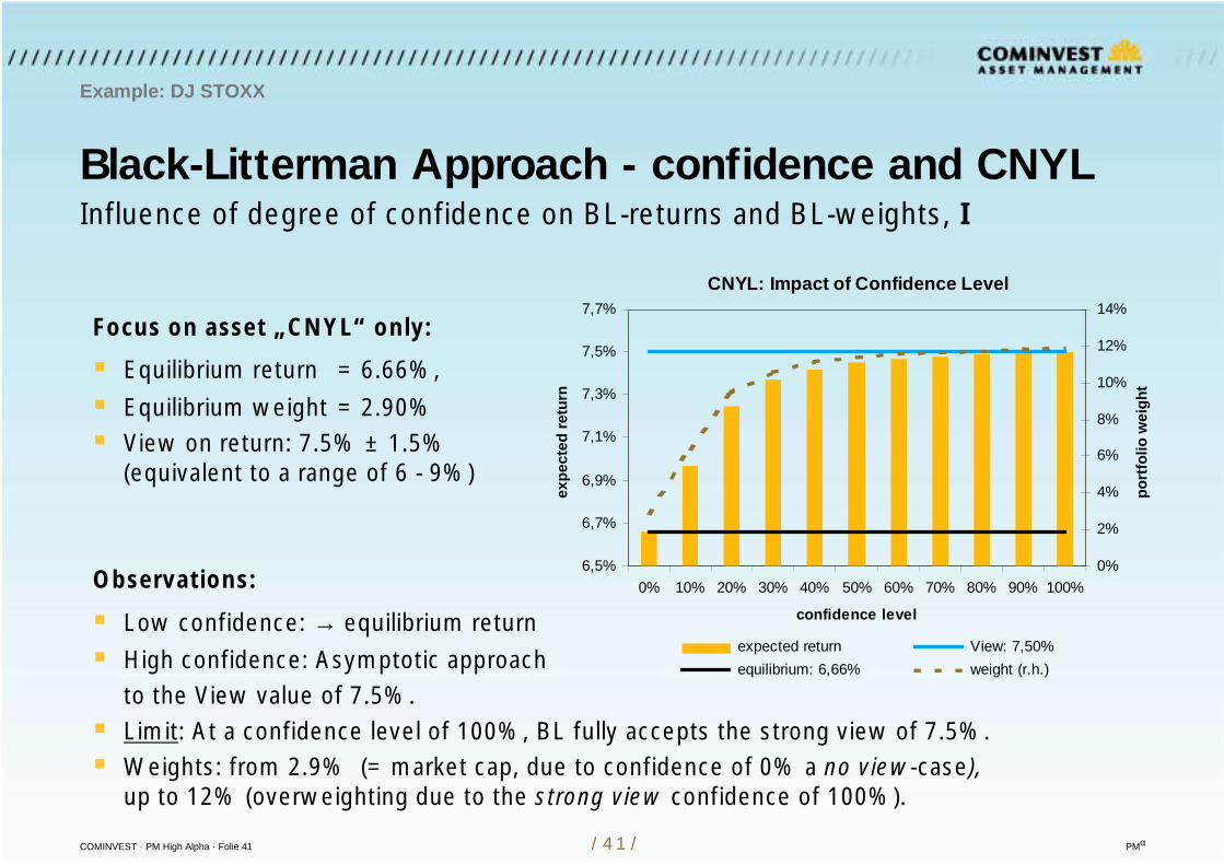
Influence of degree of confidence on BL-returns and BL-weights, I
Focus on asset „CNYL“ only:
Equilibrium return = 6.66%,
Equilibrium weight = 2.90% View on return: 7.5% ± 1.5%
(equivalent to a range of 6 - 9%)
Observations:
Low confidence: → equilibrium return
High confidence: Asymptotic approachto the View value of 7.5%.
Limit: At a confidence level of 100%, BL fully accepts the strong view of 7.5%. Weights: from 2.9% (= market cap, due to confidence of 0% a no view-case),
up to 12% (overweighting due to the strong view confidence of 100%).
CNYL: Impact of Confidence Level
6,5%
6,7%
6,9%
7,1%
7,3%
7,5%
7,7%
0% 10% 20% 30% 40% 50% 60% 70% 80% 90% 100%
confidence level
expe
cted
retu
rn0%
2%
4%
6%
8%
10%
12%
14%
port
folio
wei
ght
expected return View: 7,50% equilibrium: 6,66% weight (r.h.)
COMINVEST · PM High Alpha · Folie 42 / 42 / PMα
CNYL
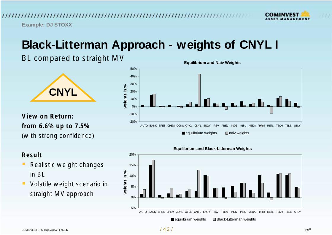
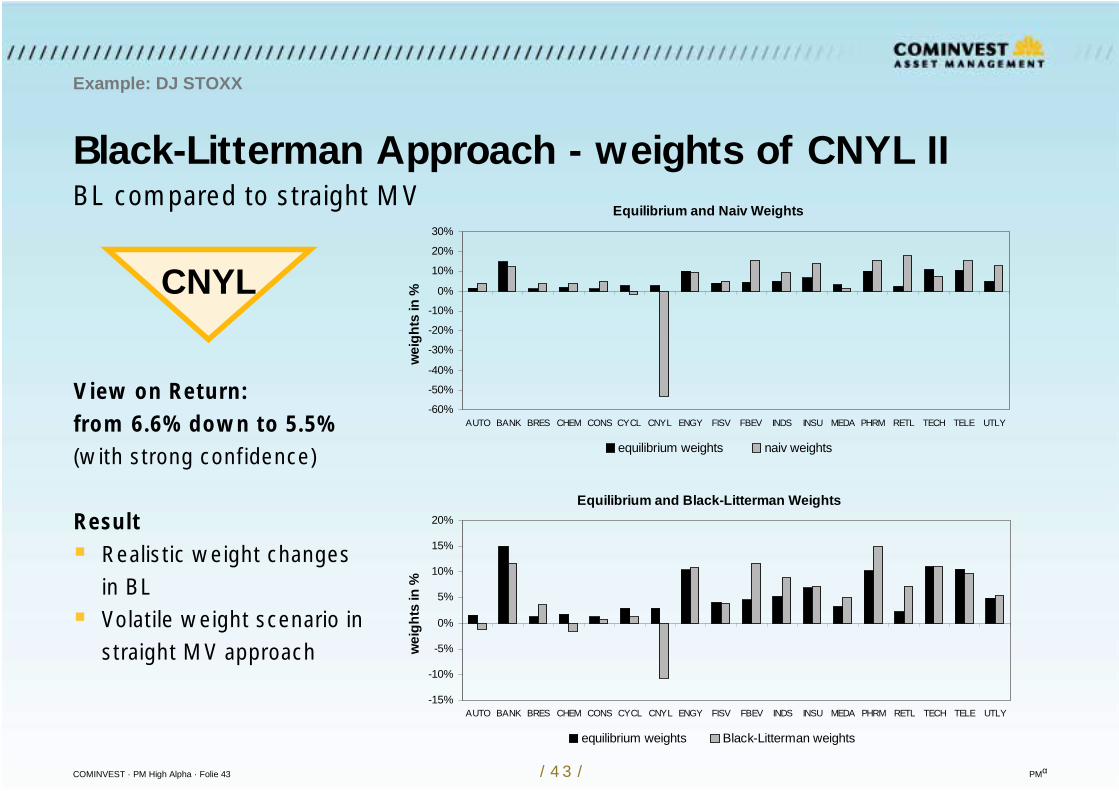
Black-Litterman Approach - weights of CNYL I
Example: DJ STOXX
View on Return:from 6.6% up to 7.5%(with strong confidence)
Result Realistic weight changes
in BL Volatile weight scenario in
straight MV approach
Equilibrium and Naiv Weights
-20%
-10%
0%
10%
20%
30%
40%
50%
AUTO BANK BRES CHEM CONS CYCL CNYL ENGY FISV FBEV INDS INSU MEDA PHRM RETL TECH TELE UTLYw
eigh
ts in
%
equilibrium weights naiv weights
Equilibrium and Black-Litterman Weights
-5%
0%
5%
10%
15%
20%
AUTO BANK BRES CHEM CONS CYCL CNYL ENGY FISV FBEV INDS INSU MEDA PHRM RETL TECH TELE UTLY
wei
ghts
in %
equilibrium weights Black-Litterman weights
BL compared to straight MV
COMINVEST · PM High Alpha · Folie 43 / 43 / PMα
CNYL
Black-Litterman Approach - weights of CNYL II
Example: DJ STOXX
View on Return:from 6.6% down to 5.5%(with strong confidence)
Result Realistic weight changes
in BL Volatile weight scenario in
straight MV approach
Equilibrium and Naiv Weights
-60%
-50%
-40%
-30%
-20%
-10%
0%
10%
20%
30%
AUTO BANK BRES CHEM CONS CYCL CNYL ENGY FISV FBEV INDS INSU MEDA PHRM RETL TECH TELE UTLYw
eigh
ts in
%
equilibrium weights naiv weights
Equilibrium and Black-Litterman Weights
-15%
-10%
-5%
0%
5%
10%
15%
20%
AUTO BANK BRES CHEM CONS CYCL CNYL ENGY FISV FBEV INDS INSU MEDA PHRM RETL TECH TELE UTLY
wei
ghts
in %
equilibrium weights Black-Litterman weights
BL compared to straight MV
COMINVEST · PM High Alpha · Folie 44 / 44 / PMα
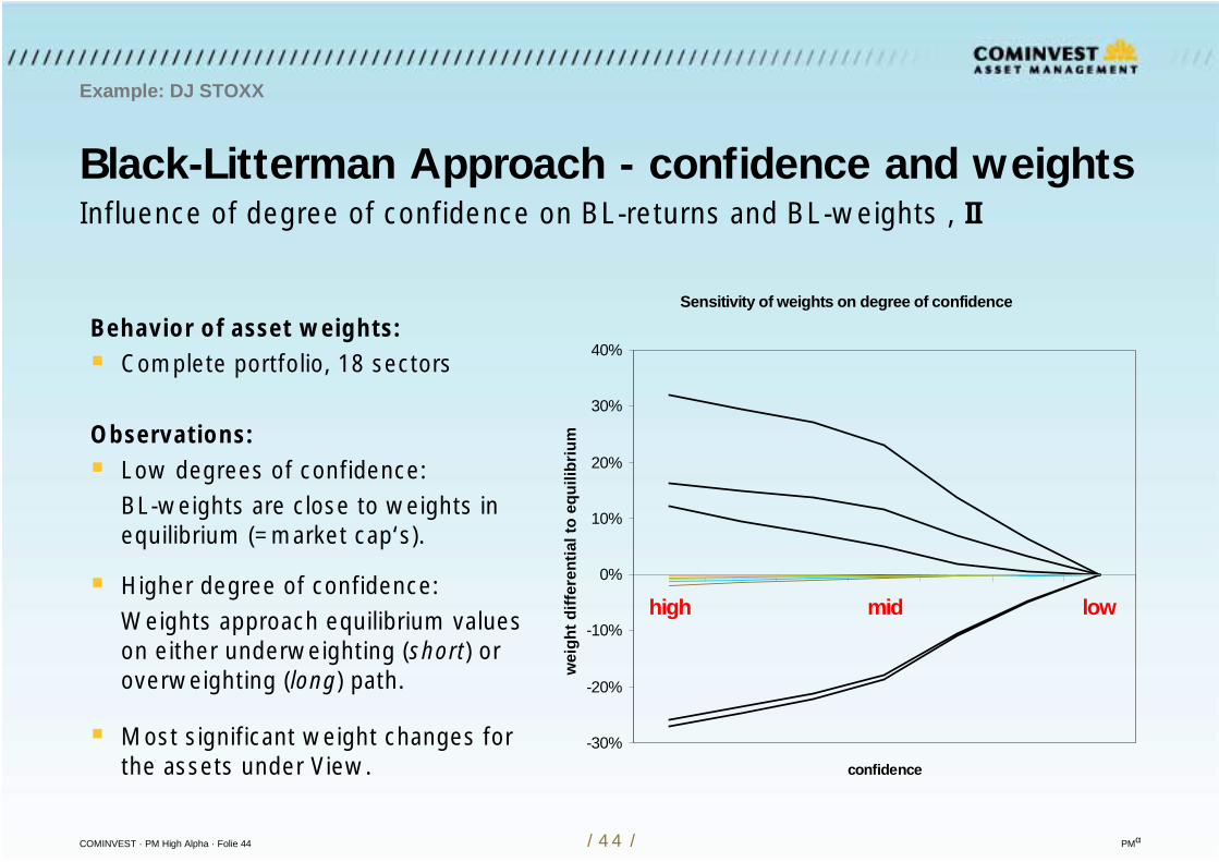
Black-Litterman Approach - confidence and weights
Example: DJ STOXX
Influence of degree of confidence on BL-returns and BL-weights , II
Behavior of asset weights: Complete portfolio, 18 sectors
Observations: Low degrees of confidence:
BL-weights are close to weights inequilibrium (=market cap‘s).
Higher degree of confidence:Weights approach equilibrium valueson either underweighting (short) oroverweighting (long) path.
Most significant weight changes forthe assets under View.
Sensitivity of weights on degree of confidence
-30%
-20%
-10%
0%
10%
20%
30%
40%
high mid low
confidence
wei
ght d
iffer
entia
l to
equi
libriu
m
COMINVEST · PM High Alpha · Folie 45 / 45 / PMα
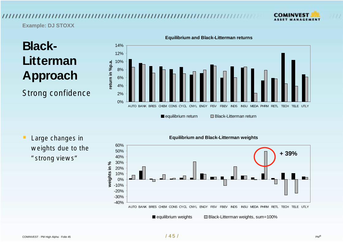
Black-LittermanApproach
Example: DJ STOXX
Large changes inweights due to the“strong views“
Strong confidence
Equilibrium and Black-Litterman returns
0%
2%
4%
6%
8%
10%
12%
14%
AUTO BANK BRES CHEM CONS CYCL CNYL ENGY FISV FBEV INDS INSU MEDA PHRM RETL TECH TELE UTLYre
turn
in %
p.a.
equilibrium return Black-Litterman return
Equilibrium and Black-Litterman weights
-40%-30%-20%-10%
0%10%20%30%40%50%60%
AUTO BANK BRES CHEM CONS CYCL CNYL ENGY FISV FBEV INDS INSU MEDA PHRM RETL TECH TELE UTLY
wei
ghts
in %
equilibrium weights Black-Litterman weights, sum=100%
+ 39%
COMINVEST · PM High Alpha · Folie 46 / 46 / PMα
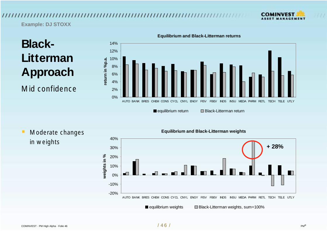
Black-LittermanApproach
Example: DJ STOXX
Moderate changesin weights
Mid confidence
Equilibrium and Black-Litterman returns
0%
2%
4%
6%
8%
10%
12%
14%
AUTO BANK BRES CHEM CONS CYCL CNYL ENGY FISV FBEV INDS INSU MEDA PHRM RETL TECH TELE UTLYre
turn
in %
p.a.
equilibrium return Black-Litterman return
Equilibrium and Black-Litterman weights
-20%
-10%
0%
10%
20%
30%
40%
AUTO BANK BRES CHEM CONS CYCL CNYL ENGY FISV FBEV INDS INSU MEDA PHRM RETL TECH TELE UTLY
wei
ghts
in %
equilibrium weights Black-Litterman weights, sum=100%
+ 28%
COMINVEST · PM High Alpha · Folie 47 / 47 / PMα
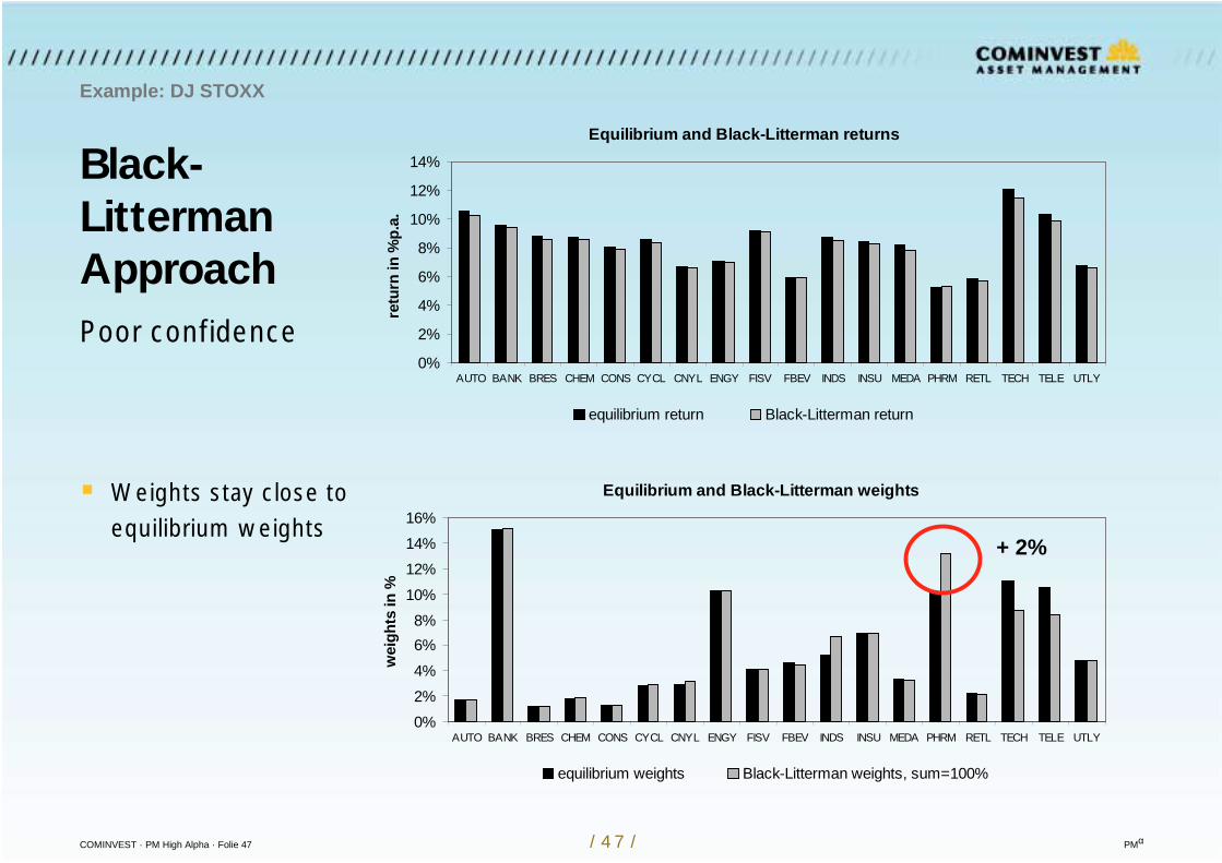
Black-LittermanApproach
Example: DJ STOXX
Weights stay close toequilibrium weights
Poor confidence
Equilibrium and Black-Litterman returns
0%
2%
4%
6%
8%
10%
12%
14%
AUTO BANK BRES CHEM CONS CYCL CNYL ENGY FISV FBEV INDS INSU MEDA PHRM RETL TECH TELE UTLYre
turn
in %
p.a.
equilibrium return Black-Litterman return
Equilibrium and Black-Litterman weights
0%2%4%6%8%
10%12%14%16%
AUTO BANK BRES CHEM CONS CYCL CNYL ENGY FISV FBEV INDS INSU MEDA PHRM RETL TECH TELE UTLY
wei
ghts
in %
equilibrium weights Black-Litterman weights, sum=100%
+ 2%
COMINVEST · PM High Alpha · Folie 48 / 48 / PMα
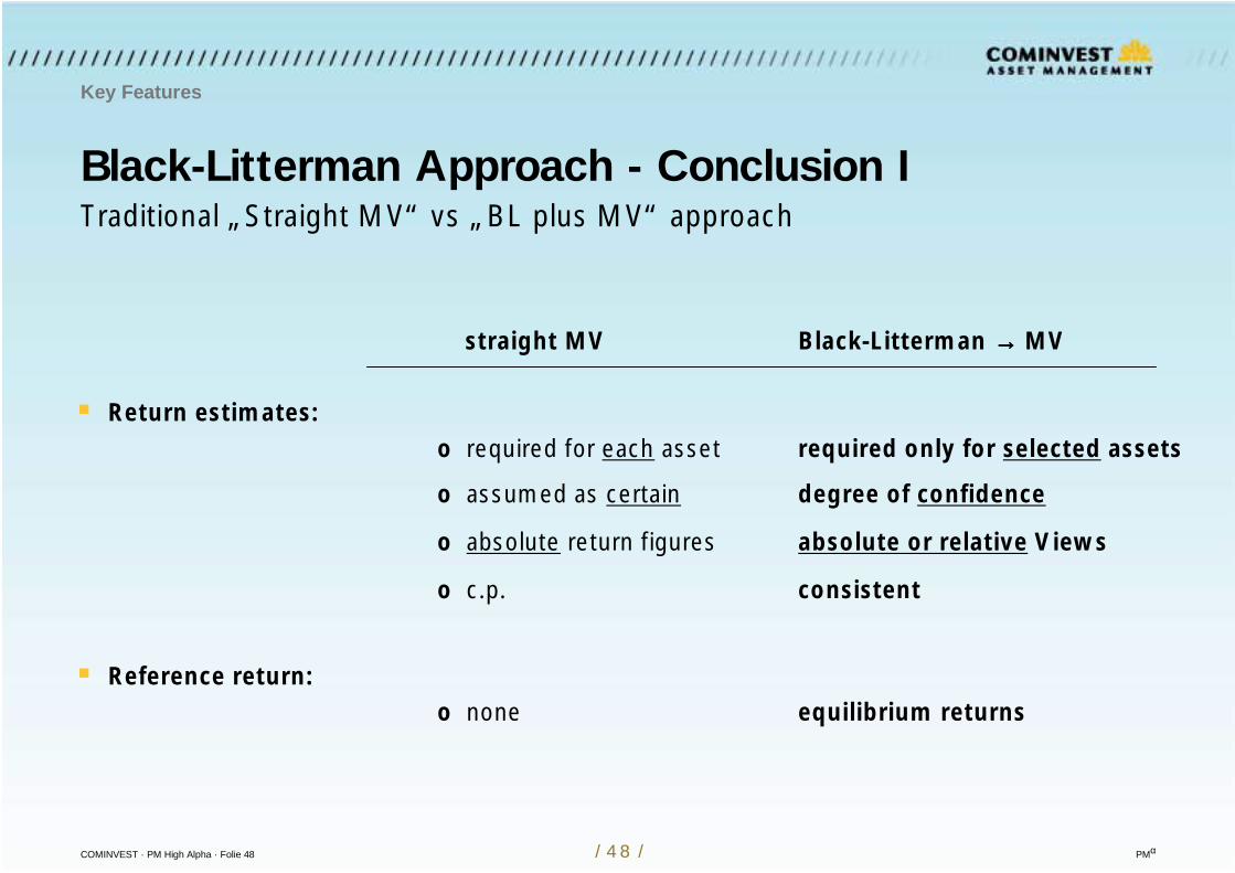
Black-Litterman Approach - Conclusion I
Key Features
Traditional „Straight MV“ vs „BL plus MV“ approach
straight MV Black-Litterman →→→→ MV
Return estimates:o required for each asset required only for selected assets
o assumed as certain degree of confidence
o absolute return figures absolute or relative Views
o c.p. consistent
Reference return:o none equilibrium returns
COMINVEST · PM High Alpha · Folie 49 / 49 / PMα
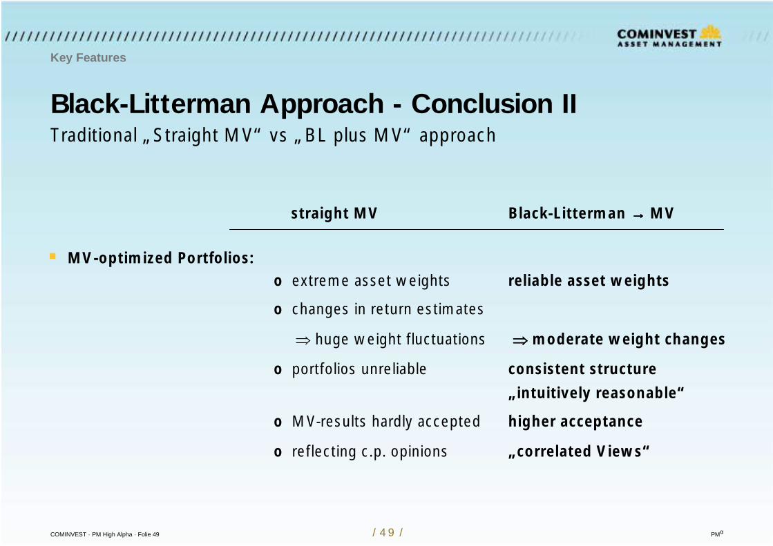
Black-Litterman Approach - Conclusion II
Key Features
Traditional „Straight MV“ vs „BL plus MV“ approach
straight MV Black-Litterman →→→→ MV
MV-optimized Portfolios:o extreme asset weights reliable asset weights
o changes in return estimates
huge weight fluctuations moderate weight changes
o portfolios unreliable consistent structure
„intuitively reasonable“
o MV-results hardly accepted higher acceptance
o reflecting c.p. opinions „correlated Views“
COMINVEST · PM High Alpha · Folie 50 / 50 / PMα
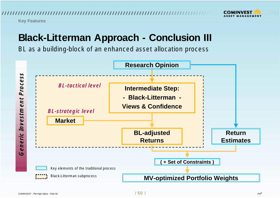
Black-Litterman Approach - Conclusion III
Key Features
BL as a building-block of an enhanced asset allocation process
Research Opinion
Intermediate Step:- Black-Litterman -Views & Confidence
BL-adjustedReturns
Market
Key elements of the traditional process
Black-Litterman subprocess
BL-tactical level
BL-strategic level
ReturnEstimates
MV-optimized Portfolio Weights
( + Set of Constraints )
Gen
eric
Inve
stm
ent
Pro
cess
COMINVEST · PM High Alpha · Folie 51 / 51 / PMα
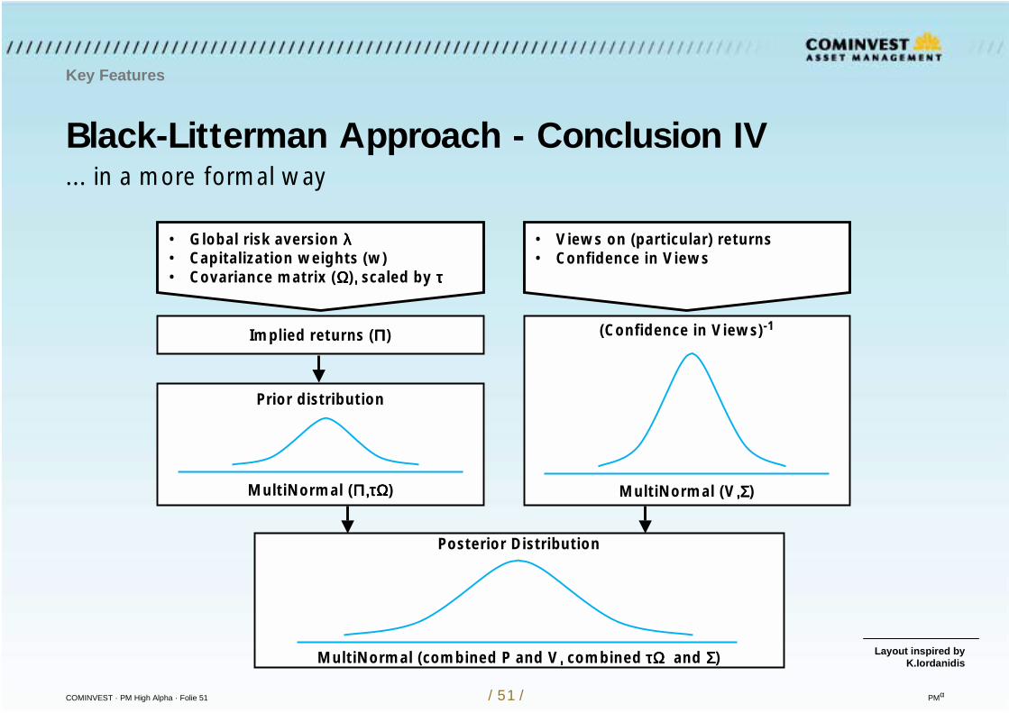
Black-Litterman Approach - Conclusion IV
Key Features
Implied returns (ΠΠΠΠ)
Prior distribution
MultiNormal (Π,τΩΠ,τΩΠ,τΩΠ,τΩ)
(Confidence in Views)-1
MultiNormal (V,Σ,Σ,Σ,Σ)
Posterior Distribution
MultiNormal (combined P and V, , , , combined τΩ τΩ τΩ τΩ and ΣΣΣΣ)
• Global risk aversion λλλλ• Capitalization weights (w)• Covariance matrix (ΩΩΩΩ), , , , scaled by ττττ
• Views on (particular) returns• Confidence in Views
Layout inspired byK.Iordanidis
... in a more formal way
COMINVEST · PM High Alpha · Folie 52 / 52 / PMα
Black-Litterman Approach - more insightsSuggestions for further reading...
Black F. and Litterman R.: Global Portfolio Optimization, Fin.Analysts Journal, Sep.1992 Black F. and Litterman R.: Asset Allocation: Combining Investor Views with Market Equilibrium,
Goldman-Sachs, Fixed Income Research, Sep.1990 Zimmermann H., Drobetz W. and Oertmann P.: Global Asset Allocation: New Methods and Applications,
publ. by Wiley & Sons, Nov.2002 Christodoulakis G.A.: Bayesian Optimal Portfolio Selection: The BL Approach, Nov.2002 He Q. and Litterman R.: The Intuition behind BL-Model Portfolios, Dec.1999 Idzorek T.: Step-by-Step Guide to the BL-Model, Feb.2002 Iordanidis K.: Global Asset Allocation: Portfolio Construction & Risk Management, Jan.2002 Fusai G. and Meucci A.: Assessing views, Risk, Mar.2003 Bevan A. and Winkelmann K.: Using the BL Global Asset Allocation Model: Three Years of Practical
Experience, Goldman-Sachs, Fixed Income Research, Jun.1998
in German:
Drobetz T.: Einsatz des BL-Verfahrens in der Asset Allocation, Working paper, Mar.2002 Zwahlen St.: Kritische Analyse des BL-Ansatzes, Seminararbeit, Uni St.Gallen-HSG, Jul.2004 Zimmermann H. et al.: Einsatz des Black-Litterman-Verfahrens in der Asset Allocation, in „Handbuch Asset
Allocation“, Editors: Dichtl, Schlenger u. Kleeberg, Uhlenbruch-Verlag, 2002.
Some literature


