
ComputerVision
Sampling, Quantization and
Image Enhancement

ComputerVision
ComputerVision Part I : Sampling & quantization
1. Discretization of continuous signals2. Signal representation in the frequency domain3. Effects of sampling and quantization
Part II : Image enhancement
1. Noise suppression 2. De-blurring3. Contrast enhancement

ComputerVision
ComputerVision Part I : Sampling & quantization
1. Discretization of continuous signals2. Signal representation in the frequency domain3. Effects of sampling and quantization
Part II : Image enhancement
1. Noise suppression 2. De-blurring3. Contrast enhancement

ComputerVision
ComputerVision Recall – photons to digital signal
• CCD : Charge-coupled device• CMOS : Complementary Metal Oxide Semiconductor• We will study the effects of the digitization / discretization.
Part I - Intro

ComputerVision
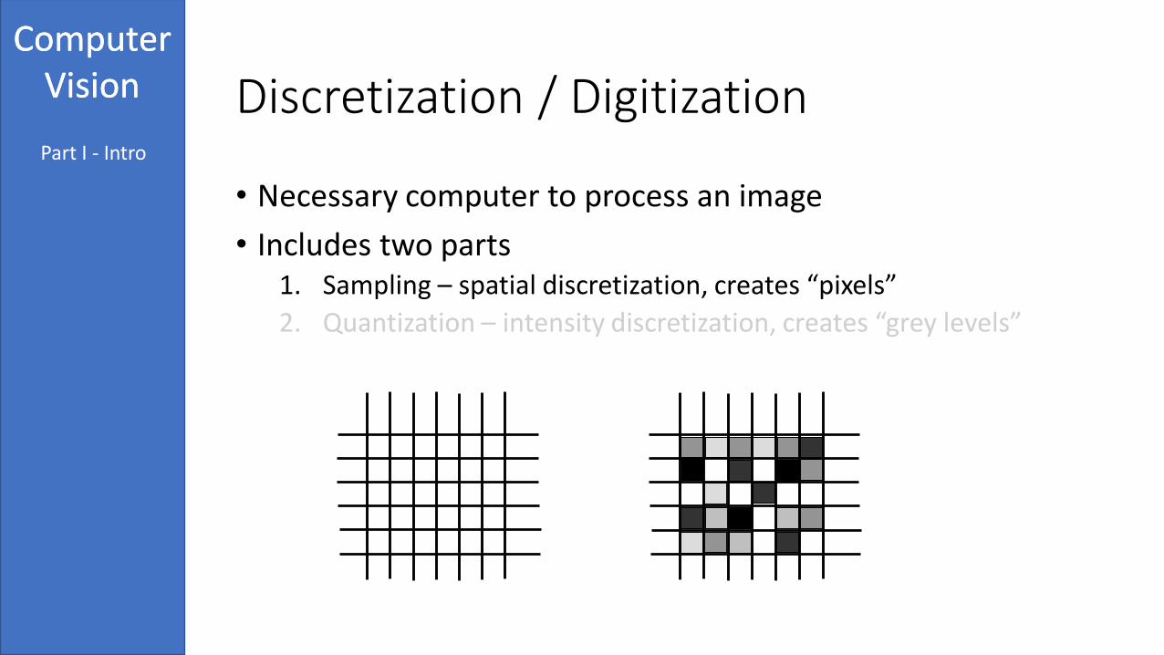
ComputerVision Discretization / Digitization
• Necessary computer to process an image
• Includes two parts 1. Sampling – spatial discretization, creates “pixels”
2. Quantization – intensity discretization, creates “grey levels”
Part I - Intro

ComputerVision
ComputerVision Sampling & Quantization
Part I – Intro
84 133 226 212 218 218 222 212 218 222 226 218
75 156 177 218 212 218 218 218 218 222 218 218
96 84 133 203 218 218 218 222 212 218 222 218
123 75 111 156 212 218 212 212 218 218 218 226
93 75 71 133 185 231 226 226 222 212 218 218
51 75 75 75 156 206 218 218 218 222 212 222
44 110 75 65 143 194 231 218 218 218 218 218
52 123 69 84 60 156 199 231 231 222 226 226
52 75 84 81 65 69 150 231 231 226 231 231
36 36 84 93 84 71 156 160 240 240 231 231
36 40 113 75 69 75 71 133 194 240 240 240
52 52 105 85 69 75 75 123 111 222 231 231
69 44 69 93 81 75 75 69 150 177 247 240
73 44 40 96 101 75 75 75 84 133 231 240
Creating finite number of points in space in a grid, i.e. pixels, and intensity value in eachpixel is represented with finite number of bits in the computer.
The original scene is continuous in space and intensity value

ComputerVision
ComputerVision Example of sampling
Part I – Intro
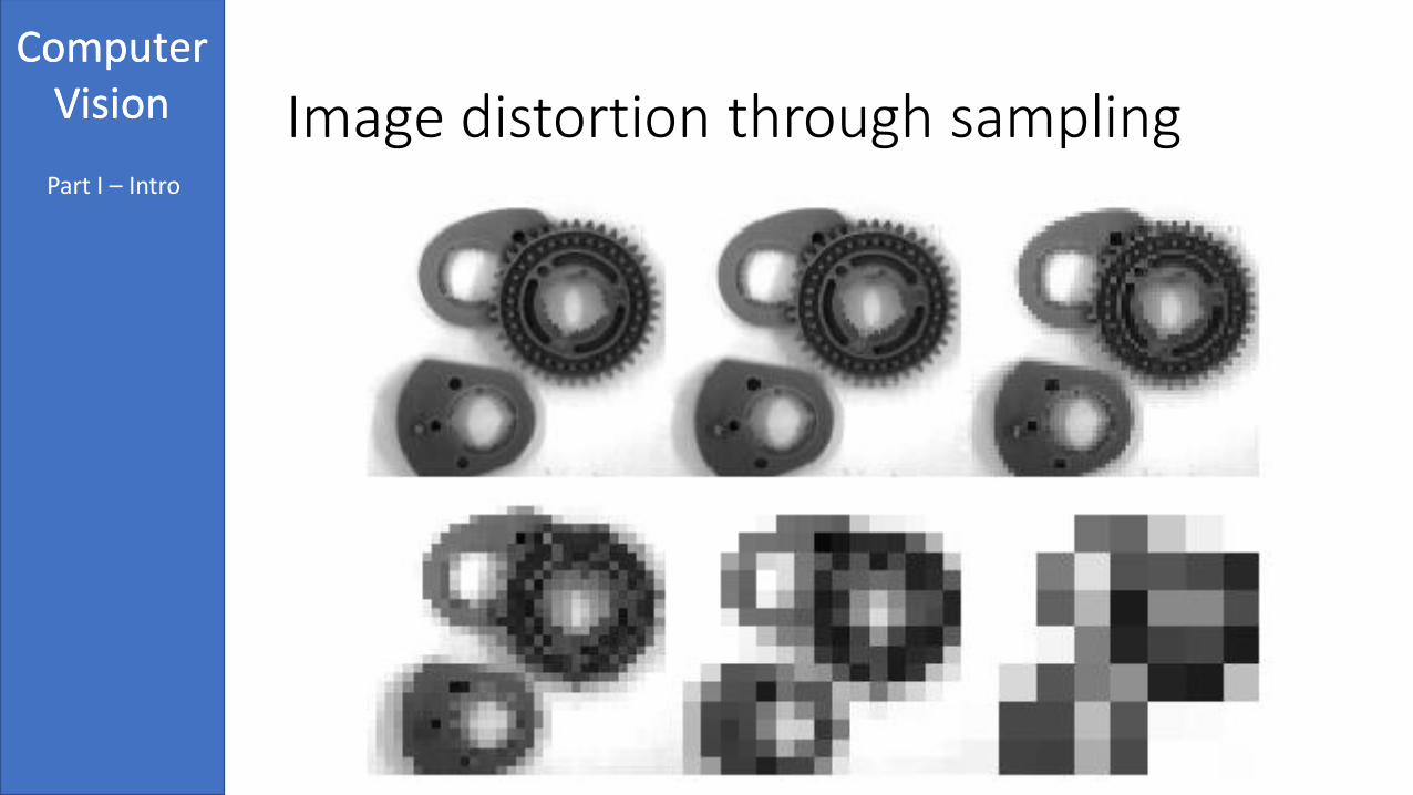
384 x 288 pixels
48 x 36 pixels92 x 72 pixels
192 x 144 pixels

ComputerVision
ComputerVision Example of quantization
Part I – Intro
2 levels - binary
256 levels – 1 byte8 levels
4 levels
ComputerVision
ComputerVision Image distortion through sampling
Part I – Intro

ComputerVision
ComputerVision Image distortion through quantization
Part I – Intro

ComputerVision
ComputerVision Remarks
1. Binary images – 1-bit quantization – are useful in industrial applications. They usually have control over imaging conditions, e.g. background color, lighting conditions, …
2. Non-uniform sampling and/or quantization is sometimes used for specialized applicationsa. Fine sampling to capture detailsb. Fine quantization for homogeneous regions
3. Different sampling strategies than square grids exist
Part I – Intro

ComputerVision
ComputerVision Different sampling schemes
• You need regular, image covering tessellation
• There are 11 polygons to achieve this. If you want to use the same polygon across the image then only 3, shown on the right.
• Rectangular (square) is the most popular
• Hexagonal has advantages (more isotropic, no connectivity ambiguities). Similar structure is seen in the retina of various species.
Part I – Intro
ComputerVision
ComputerVision Discretization / Digitization
• Necessary computer to process an image
• Includes two parts 1. Sampling – spatial discretization, creates “pixels”
2. Quantization – intensity discretization, creates “grey levels”
Part I - Intro

ComputerVision
ComputerVision A model for sampling
• There are two essential steps
1. Integrate brightness over a cell windowLeads to blurring type degradation
2. Read out values only at the pixel centersLeads to aliasing and leakage, frequency domain issues
Part I – IntroPart I – Sampling

ComputerVision
ComputerVision STEP I: integrating over a cell windowPart I – Intro
Part I – Sampling
This is a convolution:

ComputerVision
ComputerVision Convolution
• While the previous convolution was in continuous domain, we’ll look at discrete convolution to get an intuition.
Part I – IntroPart I – Sampling
Image: x(i,j)
Convolutional kernel: w(i,j)

ComputerVision
ComputerVision Convolution
• While the previous convolution was in continuous domain, we’ll look at discrete convolution to get an intuition.
Part I – IntroPart I – Sampling
Image: x(i,j)
Convolutional kernel: w(i,j)

ComputerVision
ComputerVision
Image
kernel
a b c
d e f
g h j
a cb
d fe
g jh
Part I – IntroPart I – Sampling

ComputerVision
ComputerVision Convolution
• While the previous convolution was in continuous domain, we’ll look at discrete convolution to get an intuition.
Part I – IntroPart I – Sampling
Consider the continuous case as the limit where pixels are very small as well as the convolutional kernel is formed to correspond to that with many very small elements.
The kernel for this case is a rectangular box.

ComputerVision
ComputerVision Properties of convolution
Commutative
Associative
Part I – IntroPart I – Sampling

ComputerVision
ComputerVision The Fourier Transform
• An important tool we should remind ourselves is the Fourier Transform (FT).
• This is crucial to understand the effects of STEPI as well as STEPII taken in sampling.
• Particularly, it is difficult to understand what type of information we lose when we convolve an image with a kernel with a box shape.
• Using FT, this becomes much easier!
Part I – IntroPart I – Sampling

ComputerVision
ComputerVision Characterization of functions in the
frequency domain• Represent any signal as a linear combination of orthonormal
basis functions
)( vyuxie 2 )(sin)(cos vyuxivyux 22
22
1
vu
• Waves with wavelength orthogonal to the stripes of
Part I – IntroPart I – Sampling

ComputerVision
ComputerVision The Fourier Transform: definitionPart I – Intro
Part I – Sampling Linear decomposition of functions in the new basisScaling factor for basis function (u,v)
Reconstruction of the original function in the spatialdomain: weighted sum of the basis functions
The Fourier Transform
The Inverse Fourier Transform

ComputerVision
ComputerVision Fourier Coefficients
Complex function
Magnitude
Phase - angle
Part I – IntroPart I – Sampling

ComputerVision
ComputerVision Decomposition visuallyPart I – Intro
Part I – Sampling

ComputerVision
ComputerVision Example of FTPart I – Intro
Part I – Sampling

ComputerVision
ComputerVision Effect of additional componentsPart I – Intro
Part I – Sampling

ComputerVision
ComputerVision Importance of the magnitude in FT
• Image with periodic structure
FT has peaks at spatial frequencies of repeated texture
Part I – IntroPart I – Sampling

ComputerVision
ComputerVision Importance of the magnitude in FTPart I – Intro
Part I – Sampling
Periodic background removed
remove peaks

ComputerVision
ComputerVision General structure of the magnitude
cross-section
•Magnitude generally decreases with higher spatial frequencies
•phase appears less informative
Phase
Part I – IntroPart I – Sampling

ComputerVision
ComputerVision Importance of the phase in FT
magnitude
phase phase
Part I – IntroPart I – Sampling

ComputerVision
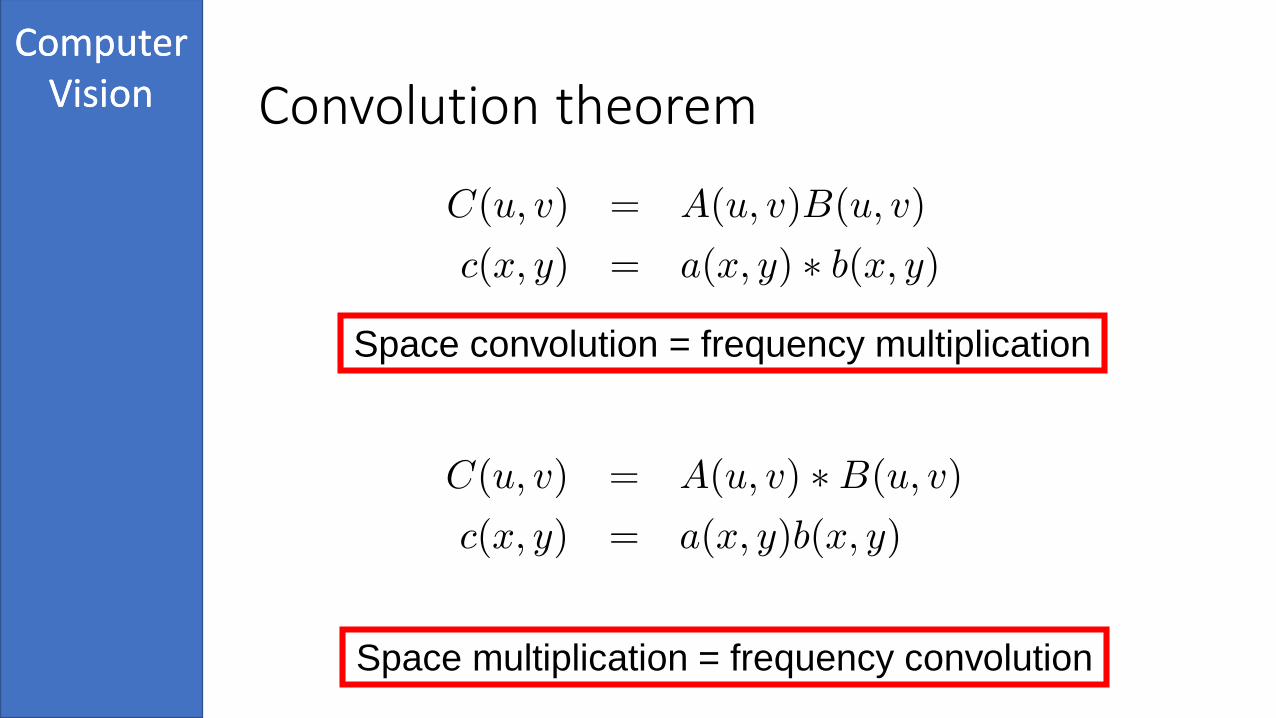
ComputerVision The convolution theoremPart I – Intro
Part I – Sampling
What is the FT of a convolution?

ComputerVision
ComputerVision The convolution theorem Part I – Intro
Part I – Sampling
Noticing the two separate FT in this four integral term leads to the main result
Space convolution = frequency multiplication

ComputerVision
ComputerVision Reciprocity in convolution theoremPart I – Intro
Part I – Sampling
Space multiplication = frequency convolution

ComputerVision
ComputerVision Point spread function and
Modulation transfer functionPart I – Intro
Part I – Sampling
modulation transfer function
• When we talk about an imaging system where there is an image i(x,y) and a kernel r(x,y) that convolves the image, it is common to call the kernel the point spread function
• The convolution spreads the intensities to adjacent pixels based on r(x,y)• Widely used terminology in microscopic imaging

ComputerVision
ComputerVision STEP I: integrating over a cell windowPart I – Intro
Part I – Sampling
This is a convolution:

ComputerVision
ComputerVision Integrating over a cell window
Assuming p(x,y) is symmetric around the originFrom convolution theorem

ComputerVision
ComputerVision Modulation transfer function of the
window function
Fourier transform of window :
2D sinc function

ComputerVision
ComputerVision Modulation transfer function – 2D sinc
real no phase shifts
predominantly low-pass
however, phase reversals !

ComputerVision
ComputerVision Illustration of the effect of 2D sinc

ComputerVision
ComputerVision Summary for STEP I
• Convolve with a window function – rectangular box
• Blurs the image
• May cause phase reversals in certain frequencies – modify the image content

ComputerVision
ComputerVision A model for sampling
• There are two essential steps
1. Integrate brightness over a cell windowLeads to blurring type degradation
2. Read out values only at the pixel centersLeads to aliasing and leakage, frequency domain issues
Part I – IntroPart I – Sampling

ComputerVision
ComputerVision Local probing of functions
To understand the effect of Step II, we need the probing function: Dirac pulse
Function probing (in 1D)
1
xx0

ComputerVision
ComputerVision Discretization in the spatial domain is
multiplication with a Dirac train2D Dirac train / Dirac comb
Fourier transform is also a Dirac train / Dirac comb
Convolution with a Dirac train: periodic repetitionYet another duality: discrete vs. periodic

ComputerVision
ComputerVision Effect on the frequency domain

ComputerVision
ComputerVision Effect on the frequency domain
1. After sampling you may not get back the original signal
2. It depends on the frequency domain representation, only band limited signals can be sampled and retrieved back
3. Even then you need to sample at a certain rate

ComputerVision
ComputerVision The sampling theorem
If the Fourier transform of a function ƒ(x,y) is zero for all
frequencies beyond ub and vb, i.e. if the Fourier transform is
band-limited, then the continuous periodic function ƒ(x,y)
can be completely reconstructed from its samples as long as
the sampling distances w and h along the x and y directions
are such that 𝑤 ≤1
2𝑢𝑏and ℎ ≤
1
2𝑣𝑏

ComputerVision
ComputerVision Summary for STEP II
• When we read off one value per pixel area, we are losing information on the image indefinitely, if the image is not band-limited, which is almost always the case.
• The information we lose is on the higher frequencies, meaning very fine details on edges, corners and texture patterns.

ComputerVision
ComputerVision Discretization / Digitization
• Necessary computer to process an image
• Includes two parts 1. Sampling – spatial discretization, creates “pixels”
2. Quantization – intensity discretization, creates “grey levels”
Part I - Intro

ComputerVision
ComputerVision Quantization
• Create K intervals in the range of possible intensities and each interval with only one value
• Measured in bits: log2(K)
• Design choices: • Decision levels / boundaries of intervals
• Representative values for each interval
• Simplest selection • Equal intervals between min and max
• Use mean in the interval as the representative value
• Uniform quantizer
• K=256 is used very often in practice

ComputerVision
ComputerVision The uniform quantizer
• Simple interpretation
• Fine quantization is needed for perceptual quality (7-8 bits)
• It can be better designed if we know what intensities we expect
• p(z) is the probability density function of intensities – constant for uniform quantizer

ComputerVision
ComputerVision Underquantization examples
256 gray level (8 bit) 11 gray level

ComputerVision
ComputerVision Small remarks on quantization
• 8 bits is often used in monochrome images
• 24 bits (8 x 3) used for RGB images per pixel
• Medical imaging may require finer quantization. 12 bits (4096 levels ) and 16 bits (65536) are often used.
• Satellite imaging also use 12 or 16 bits regularly.

ComputerVision
ComputerVision Part I : Sampling & quantization
1. Discretization of continuous signals2. Signal representation in the frequency domain3. Effects of sampling and quantization
Part II : Image enhancement
1. Noise suppression 2. De-blurring3. Contrast enhancement

ComputerVision
ComputerVision
1. Noise suppression
2. Image de-blurring
3. Contrast enhancement
Original Image Noise Blur Bad Contrast
Three types of image enhancement

ComputerVision
More on Fourier transform
Signal and noise

ComputerVision
ComputerVision The Fourier Transform: definition
Linear decomposition of functions in the new basisScaling factor for basis function (u,v)
Reconstruction of the original function in the spatialdomain: weighted sum of the basis functions
The Fourier Transform
The Inverse Fourier Transform

ComputerVision
u
v
u
v
Phase
ComputerVision
ComputerVision
Space multiplication = frequency convolution
Space convolution = frequency multiplication
Convolution theorem

ComputerVision
ComputerVision
i(x,y) ɸii = |I(u,v)|2
Amount of signal at each frequency pair
Most nearby object pixels have similar intensityMost of the signal lies in low frequencies!High frequency contains the edge information!
Images are mostly composed of homogeneous areas
Fourier power spectra of images
ComputerVision
ComputerVision
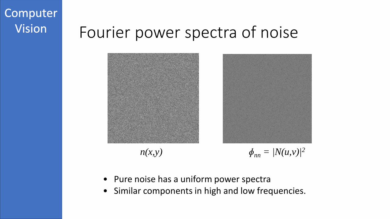
n(x,y) ɸnn = |N(u,v)|2
• Pure noise has a uniform power spectra• Similar components in high and low frequencies.
Fourier power spectra of noise

ComputerVision
ComputerVision
f(x,y) ɸff = |F(u,v)|2
Power spectra is a combination of image and noise
Fourier power spectra of noisy image

ComputerVision
ComputerVision
ɸii(u,v) / ɸnn(u,v)
High SNR
Low SNR
Low SNRLow SNR
Low SNR
Signal to noise ratio (SNR)
ComputerVision
ComputerVision
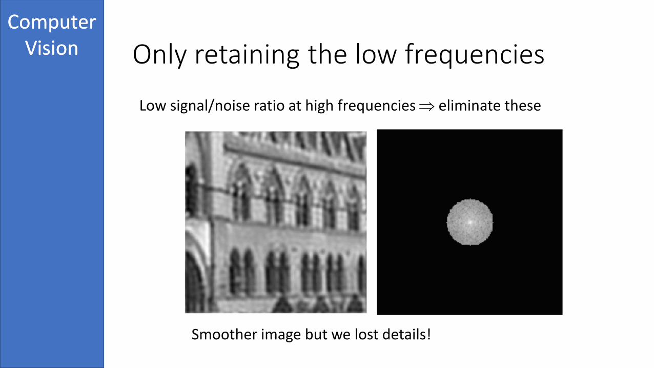
Low signal/noise ratio at high frequencies eliminate these
Smoother image but we lost details!
Only retaining the low frequencies

ComputerVision
ComputerVision
We cannot simply discard the higher frequencies
They are also introduced by edges
High frequencies contains noise and edge information

ComputerVision
ComputerVision
1. Noise suppression
2. Image de-blurring
3. Contrast enhancement
Original Image Noise Blur Bad Contrast
Three types of image enhancement

ComputerVision
Original Image Noisy Observation
NoiseSuppression

ComputerVision
ComputerVision Noise suppresion
• In general specific methods for specific types of noise
• We only consider 2 general options here:
1. Convolutional linear filters – low-pass convolutional filters
2. Non-linear filters - edge-preserving filtersa. Median
b. Anisotropic diffusion

ComputerVision
Goal: remove low-signal/noise part of the spectrum
Such spectrum filters yield “rippling”due to ripples of the spatial filter and convolution
Approach 1: Multiply the Fourier domain by a mask
Low-pass filtering - principle

ComputerVision Illustration of rippling

ComputerVision
Approach 2: Low-pass convolution filtersgenerate low-pass filters that do not cause rippling
Idea: Model convolutional filters in the spatial domain to approximate low-pass filtering in thefrequency domain
Convolutional
filterFrequency
mask
Low-pass filtering - principle
ComputerVision
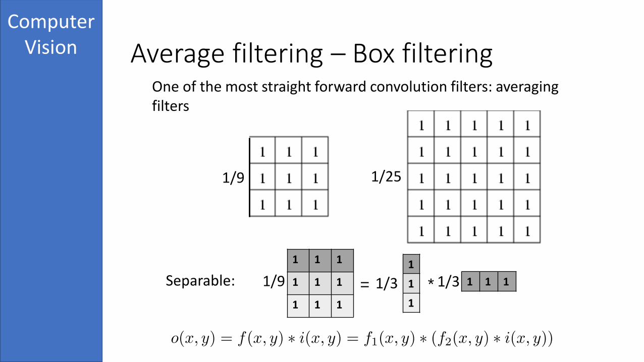
One of the most straight forward convolution filters: averaging filters
Separable:
1 1 1
1 1 1
1 1 1
=
1
1
1
1 1 1*
1/9 1/25
1/9 1/3 1/3
Average filtering – Box filtering

ComputerVision
Noise is gone.
Result is blurred!
Example for box/average filtering
ComputerVision
3 x 3 (separable!)
(1+2cos(2u)) (1+2cos(2v))
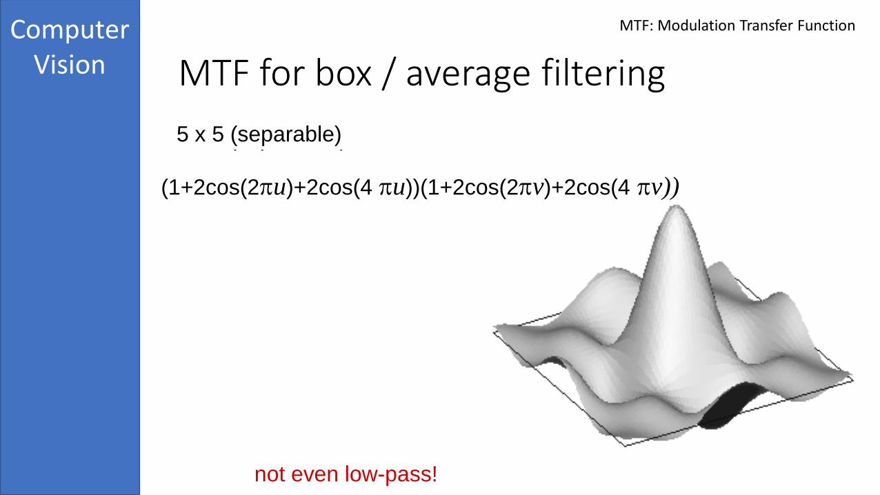
5 x 5 (separable)
(1+2cos(2u)+2cos(4 u))(1+2cos(2v)+2cos(4 v))
not even low-pass!
MTF for box / average filtering
MTF: Modulation Transfer Function

ComputerVision
1. Masking frequency domain with window type low-pass filter yields sinc-type of spatial filter and ripples -> disturbing effect
2. box filters are not exactly low-pass, ripples in the frequency domain at higher freq. remember phase reversals?
no ripples in either domain required!
So far
ComputerVision
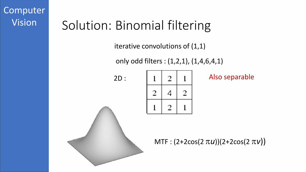
MTF : (2+2cos(2 u))(2+2cos(2 v))
iterative convolutions of (1,1)
only odd filters : (1,2,1), (1,4,6,4,1)
2D : Also separable
Solution: Binomial filtering

ComputerVision Results of binomial filtering

ComputerVision
f :
Gaussian with b controlling the amount of smoothing
Limit of binomial filtering

ComputerVision
Gaussian is limit case of binomial filters
noise gone, no ripples, but still blurred…
Actually linear filters cannot solve this problem
Gaussian smoothing

ComputerVision
• separable filters can be implemented efficiently
• large filters through multiplication in the frequency domain
• integer mask coefficients increase efficiency powers of 2 can be generated using shift operations
• In Gaussian filter increasing b (the standard deviation) leads to more smoothing and blurring
Some notes on implementation

ComputerVision
High SNR
Low SNR
Low SNRLow SNR
Low SNR
Can convolutional filters do a perfect job?
Can they separate edge information from noise in the higher frequency components?
Why?
Questions

ComputerVision
ComputerVision Noise suppresion
• In general specific methods for specific types of noise
• We only consider 2 general options here:
1. Convolutional linear filters – low-pass convolutional filters
2. Non-linear filters - edge-preserving filtersa. Median
b. Anisotropic diffusion

ComputerVision
ComputerVision Median filtering: principle
• Non-linear filter
• Simple method: 1. Rank-order neighborhood intensities in a patch of the image
2. Take middle value and assign it to the patch center
3. Go over all the image in a sliding window
• No new grey levels will emerge.

ComputerVision
advantage of this type of filter is its “odd-man-out” effect
e.g.
1,1,1,7,1,1,1,1
?,1,1,1.1,1,1,?
Median filtering – main advantage“odd-man-out”
ComputerVision
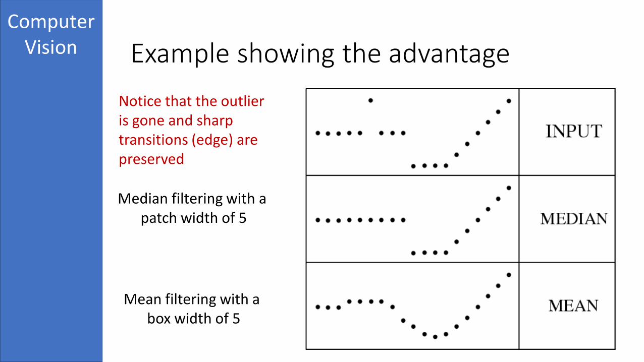
Median filtering with a patch width of 5
Mean filtering with a box width of 5
Example showing the advantage
Notice that the outlier is gone and sharp transitions (edge) are preserved

ComputerVision
• median completely discards the spike, linear filter always responds to all aspects. Great for robustness to outliers and salt-and-pepper type noise
• median filter preserves discontinuities, linear filter produces rounding-off effects. Great for preserving sharp transitions, high frequency components and, essentially, edges and corners.
• DON’T become all too optimistic
Median filtering – is it the solution to our blurring problem?

ComputerVision
3 x 3 median filter :
sharpens edges, destroys edge cusps and protrusions
Median filtering resultsComparison with Gaussian :

ComputerVision
10 times 3 X 3 median
patchy effectimportant details lost (e.g. ear-ring)
Further results

ComputerVision
For what types of noise would you clearly prefer median filtering over Gaussian filtering?
a) Gaussian noise, i.e. noise distributed by independent normal distribution
b) Salt and pepper noise
c) Uniform noise, i.e. distributed by uniform distribution
d) Exponential noise model
e) Rayleigh noise
Question

ComputerVision
ComputerVision Noise suppresion
• In general specific methods for specific types of noise
• We only consider 2 general options here:
1. Convolutional linear filters – low-pass convolutional filters
2. Non-linear filters - edge-preserving filtersa. Median
b. Anisotropic diffusion

ComputerVision
ComputerVision Anistropic diffusion: principle
• Non-linear filter
• More complicated method:
1. Gaussian smoothing across homogeneous intensity areas
2. No smoothing across edges

ComputerVision
The diffusion equation
Initial/Boundary conditions
If
in1D:
Solution is a convolution!
Gaussian filter revisited

ComputerVision
Nonlinear version can change the width of the filter locally
Specifically dependening on the edge information through gradients
Gaussian filter with time dependent standard deviation:
Diffusion as Gaussian low-pass filter

ComputerVision
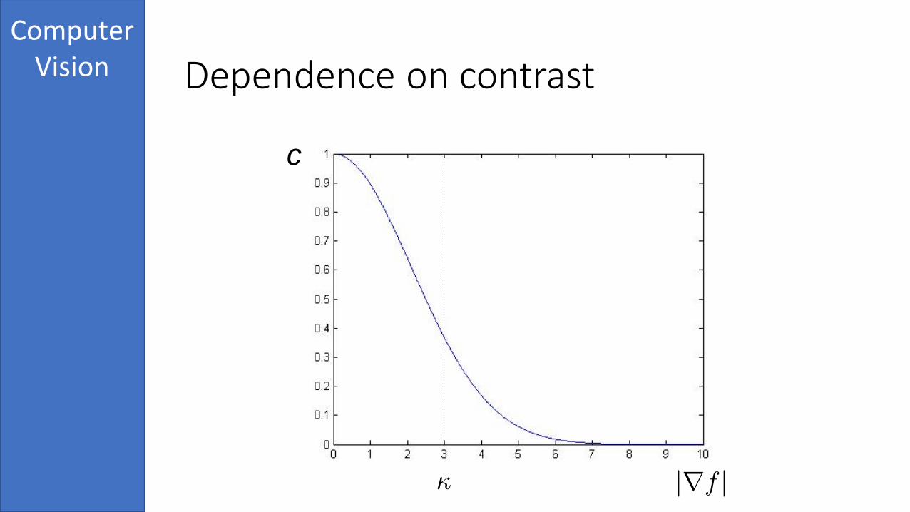
or
controls the contrast to be preserved by smootingactually edge sharpening happens
Selection of diffusion coefficient
ComputerVision
c
Dependence on contrast

ComputerVision
ComputerVision
Noisy image Ideal image
After 50 iter After 1000 iter

ComputerVision
ComputerVision
Noisy image Ideal image
After 50 iter Isotropic

ComputerVision
End state is homogeneous
Unrestrained anisotropic diffusion

ComputerVision
adding restraining force :
Restraining anisotropic diffusion

ComputerVision
Noisy image Binomial 7x7
Median 5x5 Aniso Diff. wr

ComputerVision
When c is not a constant solution is found
through solving the equation
Partial differential equation
• Numerical solutions through discretizing the differential
operators and integrating
• Finite differences in space and integration in time
Anisotropic diffusion – numerical solutions

ComputerVision
Original ImageWhat we want
Blurred imageWhat we observe
Deblurring

ComputerVision
• simple but effective method
• image independent
• linear
• used e.g. in photocopiers and scanners
Approach I: Unsharp masking

ComputerVision
red = original
black = smoothed
orginal –smooth
original +difference
Unsharp masking - sketch

ComputerVision
Interpret blurred image as snapshot of diffusion process
)( 2 fct
f
In a first order approximation, we can write
tt
fyxftyxf
)0,,(),,(
Hence,
fcttyxftt
ftyxfyxf 2),,(),,()0,,(
Unsharp masking produces o from i
ikio 2
with k a well-chosen constant
Unsharp masking - principle

ComputerVision
DOG (Difference-of-Gaussians) approximation for Laplacian :
Our 1D example: Convolution mask in 2D:
Need to estimate

ComputerVision
ikio 2
The edge profile becomes steeper, giving a sharper impression
Under-and overshoots flanking the edge further increase the
impression of image sharpness
Unsharp masking analysis

ComputerVision Unsharp masking results

ComputerVision
• Relies on system view of image processing
• Frequency domain technique
• Defined through Modulation Transfer Function
• Links to theoretically optimal approaches
Approach II: Inverse filtering

ComputerVision
Frequency domain technique
suppose you know the MTF B(u,v) of the blurring filter
to undo its effect new filter with MTF B’ (u,v) such that
Inverse filtering principle

ComputerVision
For additive noise after filtering
Result of inverse filter
Inverse filtering principle

ComputerVision
• Frequencies with B (u,v) = 0
Information fully lost during filteringCannot be recoveredInverse filter is ill-defined
• Also problem with noise added after filtering
B(u,v) is low = 1/B(u,v) is high, VERY strong noise amplification
Inverse problem’s main issue

ComputerVision
*
xx
x
1D example
ComputerVision
x x
x x
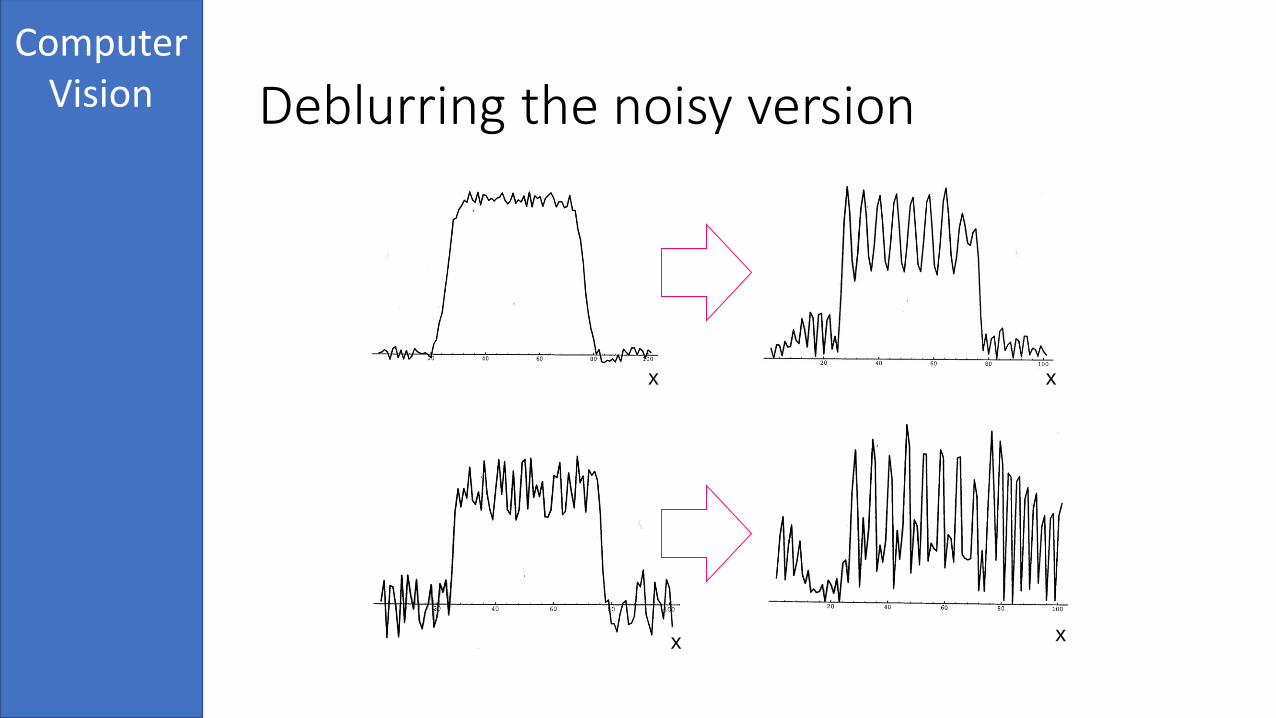
Deblurring the noisy version

ComputerVision
we will apply the method to a Gaussian smoothed example ( = 16 pixels)
Inverse filtering example on an image

ComputerVision
noise leads to spurious high frequencies
Result

ComputerVision
• Looking for the optimal filter to do the deblurring
• Consider the noise to avoid amplification
• A much better version of inverse filtering
• Optimization formulation
• Filter is given analytically in the Fourier Domain
Wiener filter

ComputerVision
•
•
•
Wiener filter and its behavior

ComputerVision
Medium confidence – medium SNR assumption
High confidence – high SNR assumption
x
x
Deblurring noise-free signal

ComputerVision
Medium confidence
Correct SNR
High confidenceLow confidence
Deblurring noisy signal

ComputerVision
spurious high freq. eliminated, conservative
Wiener filtering example

ComputerVision
• Conservative if SNR is low tends to become low-pass blurring instead of sharpening
• SNR = Φii(u,v)/Φnn(u,v) depends on I(u,v) strictly speaking is unknown
• H(u,v) must be known very precisely
is the effective filter (should be 1)
Problems in applying Wiener filtering

ComputerVision
Original Image Observationwith
Bad Contrast
Contrast Enhancement

ComputerVision
ComputerVision Contrast Enhancement
• Two use cases:
1. Compensating under-, over-exposure
2. Spending intensity range on interesting part of the image
• We will study histogram equalization

ComputerVision
Histogram
Cumulative histogram
Intensity distributions - histogram

ComputerVision
Generic transformation function
Old intensity
New
inte
nsi
ty
Power law transformation
Inew = Ioldγ
Usually monotonic mappings required
Intensity mappings

ComputerVision
WHAT : create a flat histogram
HOW :apply an appropriate intensity map
depending on the image content
method will be generally applicable
Flat histogram
Cumulative histogram
Histogram equalization

ComputerVision Histogram equalization example

ComputerVision Histogram equalization example

ComputerVision
Redistribute the intensities, 1-to-several (1-to-1 in the continuous case)
and keeping their relative order, as to use them more evenly
Ideally, obtain a constant, flat histogram
0 0
maximaxi
Histogram equalization - principle

ComputerVision
This mapping is easy to find:
It corresponds to the cumulative intensity probability or cumulative
histogram
Histogram equalization - algorithm
Histogram Cumulative histogram

ComputerVision
C’ C
1
0
intensity intensity
ii’ maximaxi
Cumulative probability
actual cum.
probability
target cum.
probability
Algorithm sketch

ComputerVision
suppose continuous probability density of original intensities i:
Mathematical justification in continuous case
Our mapping
Probability density of the transformed intensities are given as
Indeed a flat distribution!


