
CompSci 516Data Intensive Computing Systems
Lecture 9Join Algorithms
and Query Optimizations
Instructor: Sudeepa Roy
1Duke CS, Spring 2016 CompSci 516: Data Intensive Computing Systems
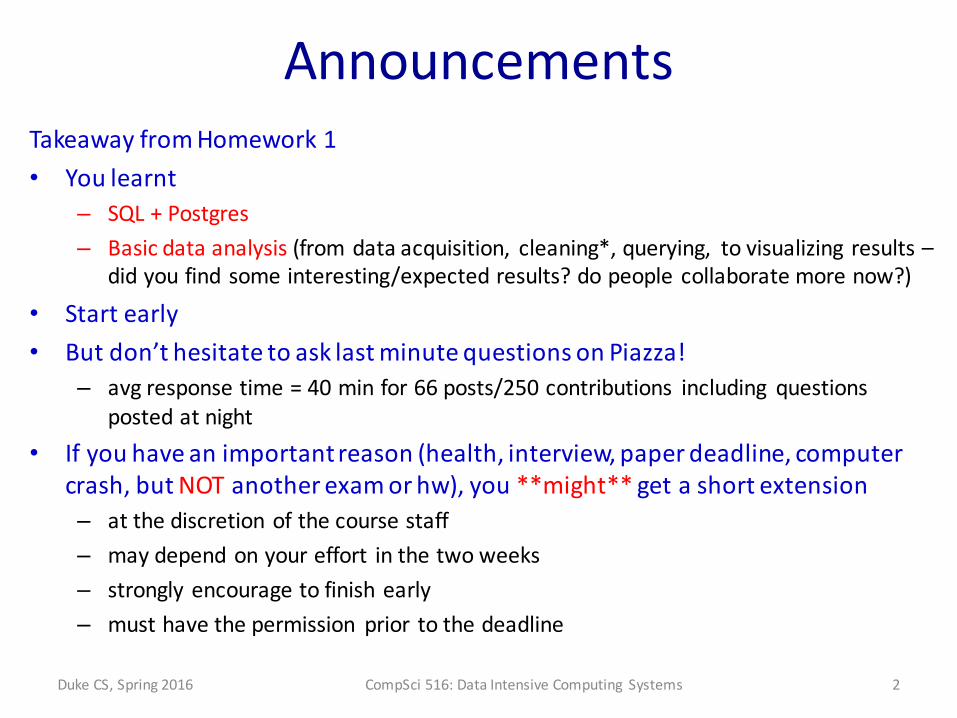
AnnouncementsTakeaway from Homework 1• You learnt
– SQL + Postgres– Basic data analysis (from data acquisition, cleaning*, querying, to visualizing results –
did you find some interesting/expected results? do people collaborate more now?)
• Start early• But don’t hesitate to ask last minute questions on Piazza!
– avg response time = 40 min for 66 posts/250 contributions including questions posted at night
• If you have an important reason (health, interview, paper deadline, computer crash, but NOT another exam or hw), you **might** get a short extension– at the discretion of the course staff– may depend on your effort in the two weeks– strongly encourage to finish early– must have the permission prior to the deadline
2Duke CS, Spring 2016 CompSci 516: Data Intensive Computing Systems

Announcements
• Homework 2– To be posted soon, due after 2 weeks– No coding, Q/A on all topics so far
• Homework 3– Part 1 will be posted soon too– Due 2 weeks **after** the due date of HW2 (in ~4 weeks)– You will learn Spark/Scala– Which will be useful when you do an assignment on AWS using Spark/Scala in HW4
3Duke CS, Spring 2016 CompSci 516: Data Intensive Computing Systems

What will we learn?
• Last lecture:– External sorting (limited buffer pages)– Operator Algorithms for Selection and Projection
• Next:– Join Algorithms– Other operators (set, aggregate)– Query Optimization
4
to be continued in the next lecture with Cost-‐based optimization and Selinger’s algorithm
Duke CS, Spring 2016 CompSci 516: Data Intensive Computing Systems

Reading Material
• [RG] – Join Algorithm: Chapter 14.4– Set/Aggregate: Chapter 14.5, 14.6– Query optimization: Chapter 15 (overview only)
5
Acknowledgement: The following slides have been created adapting theinstructor material of the [RG] book provided by the authorsDr. Ramakrishnan and Dr. Gehrke.
Duke CS, Spring 2016 CompSci 516: Data Intensive Computing Systems

Algorithms for Joins
6Duke CS, Spring 2016 CompSci 516: Data Intensive Computing Systems
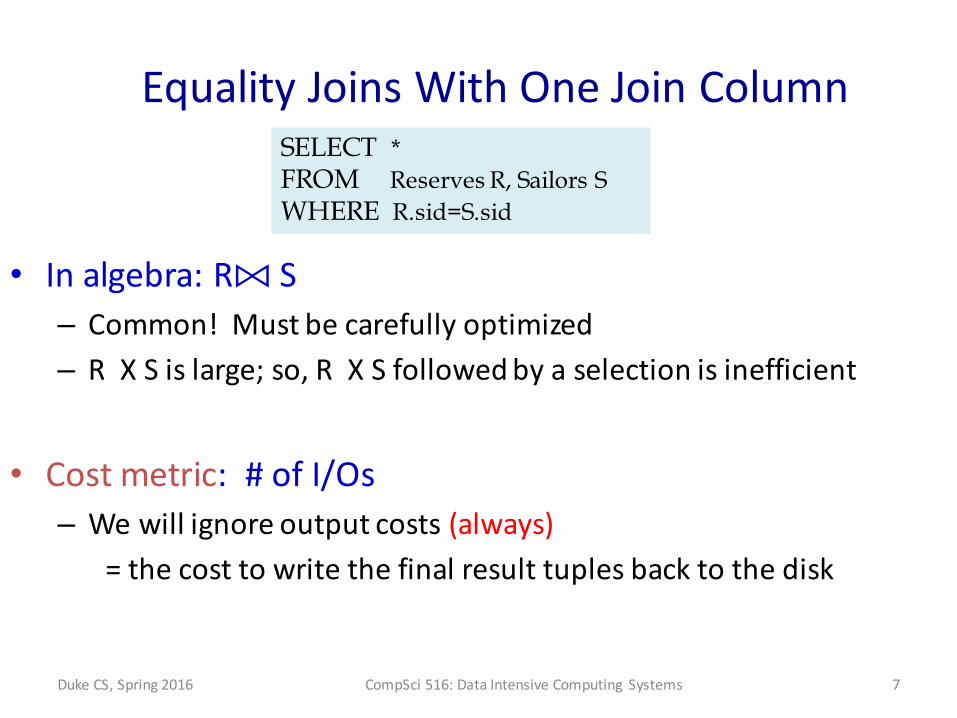
Equality Joins With One Join Column
• In algebra: R⨝ S– Common! Must be carefully optimized– R X S is large; so, R X S followed by a selection is inefficient
• Cost metric: # of I/Os– We will ignore output costs (always)
= the cost to write the final result tuples back to the disk
SELECT *FROM Reserves R, Sailors SWHERE R.sid=S.sid
7Duke CS, Spring 2016 CompSci 516: Data Intensive Computing Systems

Common Join Algorithms
1. Nested Loops Joins– Simple nested loop join– Block nested loop join– index nested loop join
2. Sort Merge Join
3. Hash Join
8
Very similar to external sort
Very similar to duplicate elimination in projection
Duke CS, Spring 2016 CompSci 516: Data Intensive Computing Systems

Algorithms for Joins
9
1. NESTED LOOP JOINS
Duke CS, Spring 2016 CompSci 516: Data Intensive Computing Systems
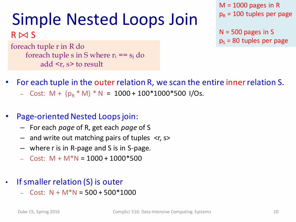
Simple Nested Loops Join
• For each tuple in the outer relation R, we scan the entire inner relation S. – Cost: M + (pR * M) * N = 1000 + 100*1000*500 I/Os.
• Page-‐oriented Nested Loops join: – For each page of R, get each page of S– and write out matching pairs of tuples <r, s>– where r is in R-‐page and S is in S-‐page.– Cost: M + M*N = 1000 + 1000*500
• If smaller relation (S) is outer– Cost: N + M*N = 500 + 500*1000
foreach tuple r in R doforeach tuple s in S where ri == sj do
add <r, s> to result
R ⨝ S
M = 1000 pages in RpR = 100 tuples per page
N = 500 pages in SpS = 80 tuples per page
10Duke CS, Spring 2016 CompSci 516: Data Intensive Computing Systems
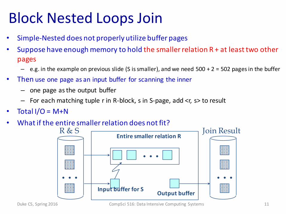
Block Nested Loops Join• Simple-‐Nested does not properly utilize buffer pages• Suppose have enough memory to hold the smaller relation R + at least two other
pages– e.g. in the example on previous slide (S is smaller), and we need 500 + 2 = 502 pages in the buffer
• Then use one page as an input buffer for scanning the inner – one page as the output buffer– For each matching tuple r in R-‐block, s in S-‐page, add <r, s> to result
• Total I/O = M+N• What if the entire smaller relation does not fit?
. . .. . .
R & SEntire smaller relation R
Input buffer for S Output buffer
. . .
Join Result
11Duke CS, Spring 2016 CompSci 516: Data Intensive Computing Systems

• If R does not fit in memory,– Use one page as an input buffer for scanning the inner S– one page as the output buffer– and use all remaining pages to hold `block’’ of outer R.– For each matching tuple r in R-‐block, s in S-‐page, add <r, s> to result– Then read next R-‐block, scan S, etc.
. . .. . .
R & SHash table for block of R
(k <= B-‐2 pages)
Input buffer for S Output buffer
. . .
Join Result
Block Nested Loops Join
12Duke CS, Spring 2016 CompSci 516: Data Intensive Computing Systems

Cost of Block Nested Loopsin class• R is outer• B-‐2 = 100-‐page blocks• How many blocks of R?• Cost to scan R?• Cost to scan S?• Total Cost?
. . .. . .
R & SHash table for block of R
(k <= B-‐2 pages)
Input buffer for S Output buffer
. . .
Join Result
foreach block of B-2 pages of R doforeach page of S do {
for all matching in-memory tuples r in R-block and s in S-page
add <r, s> to result
M = 1000 pages in RpR = 100 tuples per page
N = 500 pages in SpS = 80 tuples per page
13Duke CS, Spring 2016 CompSci 516: Data Intensive Computing Systems

Cost of Block Nested Loops• R is outer• B-‐2 = 100-‐page blocks• How many blocks of R? 10• Cost to scan R? 1000• Cost to scan S? 10 * 500• Total Cost? 1000 + 5000 = 6000• (check yourself)
• If space for just 90 pages of R, we would scan S 12 times, cost = 7000
. . .. . .
R & SHash table for block of R
(k <= B-‐2 pages)
Input buffer for S Output buffer
. . .
Join Result
foreach block of B-2 pages of R doforeach page of S do {
for all matching in-memory tuples r in R-block and s in S-page
add <r, s> to result
• Cost: Scan of outer + #outer blocks * scan of inner– #outer blocks = ⌈#pages of outer relation/blocksize⌉
M = 1000 pages in RpR = 100 tuples per page
N = 500 pages in SpS = 80 tuples per page
for blocked access, it might be goodto equally dividebuffer pagesamong R and S 14Duke CS, Spring 2016 CompSci 516: Data Intensive Computing Systems

Index Nested Loops Join
• Suppose there is an index on the join column of one relation– say S– can make it the inner relation and exploit the index– Cost: M + ( (M*pR) * cost of finding matching S tuples) – For each R tuple, cost of probing S index (get k*) is about 1.2 for hash index, 2-‐4 for B+ tree.
– Cost of then finding S tuples (assuming Alt. 2 or 3) depends on clustering• (see previous lecture)
foreach tuple r in R doforeach tuple s in S where ri == sj do
add <r, s> to result
M = 1000 pages in RpR = 100 tuples per page
N = 500 pages in SpS = 80 tuples per page
15Duke CS, Spring 2016 CompSci 516: Data Intensive Computing Systems

Cost of Index Nested Loops
• Hash-‐index (Alt. 2) on sid of Sailors (as inner), sid is a key
• Cost to scan Reserves? – 1000 page I/Os, 100*1000 tuples.
• Cost to find matching Sailors tuples?– For each Reserves tuple: – 1.2 I/Os to get data entry in index– + 1 I/O to get (the exactly one) matching Sailors tuple
• Total cost: • 1000 + 100 * 1000 * 2.2 = 221,000 I/Os
M = 1000 pages in RpR = 100 tuples per page
N = 500 pages in SpS = 80 tuples per page
foreach tuple r in R doforeach tuple s in S where ri == sj do
add <r, s> to result
SELECT *FROM Reserves R, Sailors SWHERE R.sid=S.sid
16Duke CS, Spring 2016 CompSci 516: Data Intensive Computing Systems

Cost of Index Nested Loops
• Hash-‐index (Alt. 2) on sid of Reserves (as inner), sid is NOT a key
• Cost to Scan Sailors: – 500 page I/Os, 80*500 tuples.
• For each Sailors tuple: – 1.2 I/Os to find index page with data entries– + cost of retrieving matching Reserves tuples
• Assuming uniform distribution, 2.5 reservations per sailor (100,000 / 40,000). • Cost of retrieving them is 1 or 2.5 I/Os depending on whether the index is clustered
• Total cost = 500 + 80 * 500 * 2.2 if clustered• up to ~ 500 + 80 * 500 * 3.7 if unclustered (approx)
M = 1000 pages in RpR = 100 tuples per page
N = 500 pages in SpS = 80 tuples per page
foreach tuple r in R doforeach tuple s in S where ri == sj do
add <r, s> to result
SELECT *FROM Reserves R, Sailors SWHERE R.sid=S.sid
17Duke CS, Spring 2016 CompSci 516: Data Intensive Computing Systems

Algorithms for Joins
18
2. SORT-‐MERGE JOINS
Duke CS, Spring 2016 CompSci 516: Data Intensive Computing Systems

Sort-‐Merge Join
• Sort R and S on the join column• Then scan them to do a ``merge’’ (on join col.)• Output result tuples.
19Duke CS, Spring 2016 CompSci 516: Data Intensive Computing Systems
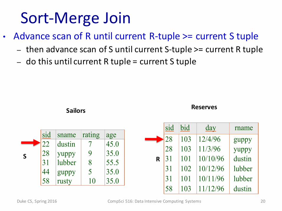
Sort-‐Merge Join
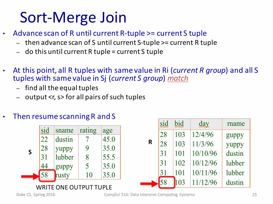
sid sname rating age22 dustin 7 45.028 yuppy 9 35.031 lubber 8 55.544 guppy 5 35.058 rusty 10 35.0
sid bid day rname28 103 12/4/96 guppy28 103 11/3/96 yuppy31 101 10/10/96 dustin31 102 10/12/96 lubber31 101 10/11/96 lubber58 103 11/12/96 dustin
Sailors
R
• Advance scan of R until current R-‐tuple >= current S tuple– then advance scan of S until current S-‐tuple >= current R tuple– do this until current R tuple = current S tuple
20Duke CS, Spring 2016 CompSci 516: Data Intensive Computing Systems
Reserves
S
Sort-‐Merge Join
sid sname rating age22 dustin 7 45.028 yuppy 9 35.031 lubber 8 55.544 guppy 5 35.058 rusty 10 35.0
sid bid day rname28 103 12/4/96 guppy28 103 11/3/96 yuppy31 101 10/10/96 dustin31 102 10/12/96 lubber31 101 10/11/96 lubber58 103 11/12/96 dustin
S R
WRITE TWO OUTPUT TUPLES
• Advance scan of R until current R-‐tuple >= current S tuple– then advance scan of S until current S-‐tuple >= current R tuple– do this until current R tuple = current S tuple
• At this point, all R tuples with same value in Ri (current R group) and all S tuples with same value in Sj (current S group) match– find all the equal tuples– output <r, s> for all pairs of such tuples
21Duke CS, Spring 2016 CompSci 516: Data Intensive Computing Systems

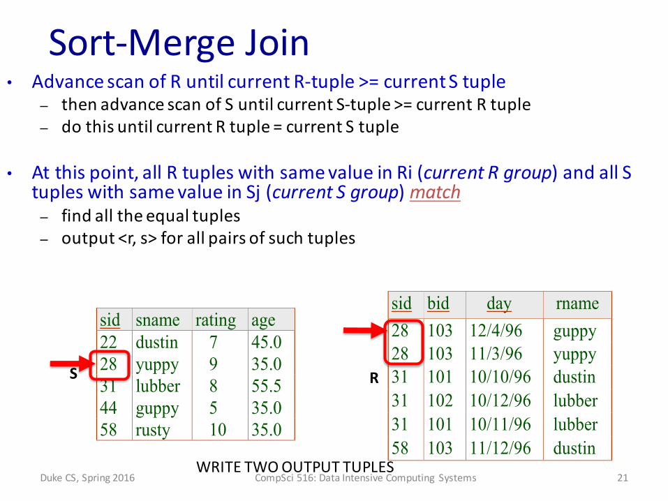
Sort-‐Merge Join
sid sname rating age22 dustin 7 45.028 yuppy 9 35.031 lubber 8 55.544 guppy 5 35.058 rusty 10 35.0
sid bid day rname28 103 12/4/96 guppy28 103 11/3/96 yuppy31 101 10/10/96 dustin31 102 10/12/96 lubber31 101 10/11/96 lubber58 103 11/12/96 dustin
SR
• Advance scan of R until current R-‐tuple >= current S tuple– then advance scan of S until current S-‐tuple >= current R tuple– do this until current R tuple = current S tuple
• At this point, all R tuples with same value in Ri (current R group) and all S tuples with same value in Sj (current S group) match– find all the equal tuples– output <r, s> for all pairs of such tuples
• Then resume scanning R and S
22Duke CS, Spring 2016 CompSci 516: Data Intensive Computing Systems
Sort-‐Merge Join
sid sname rating age22 dustin 7 45.028 yuppy 9 35.031 lubber 8 55.544 guppy 5 35.058 rusty 10 35.0
sid bid day rname28 103 12/4/96 guppy28 103 11/3/96 yuppy31 101 10/10/96 dustin31 102 10/12/96 lubber31 101 10/11/96 lubber58 103 11/12/96 dustin
SR
WRITE THREE OUTPUT TUPLES
• Advance scan of R until current R-‐tuple >= current S tuple– then advance scan of S until current S-‐tuple >= current R tuple– do this until current R tuple = current S tuple
• At this point, all R tuples with same value in Ri (current R group) and all S tuples with same value in Sj (current S group) match– find all the equal tuples– output <r, s> for all pairs of such tuples
• Then resume scanning R and S
23Duke CS, Spring 2016 CompSci 516: Data Intensive Computing Systems
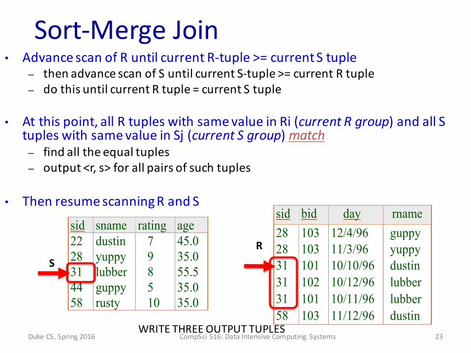
Sort-‐Merge Join
sid sname rating age22 dustin 7 45.028 yuppy 9 35.031 lubber 8 55.544 guppy 5 35.058 rusty 10 35.0
sid bid day rname28 103 12/4/96 guppy28 103 11/3/96 yuppy31 101 10/10/96 dustin31 102 10/12/96 lubber31 101 10/11/96 lubber58 103 11/12/96 dustin
SR
NO MATCH, CONTINUE SCANNING R
• Advance scan of R until current R-‐tuple >= current S tuple– then advance scan of S until current S-‐tuple >= current R tuple– do this until current R tuple = current S tuple
• At this point, all R tuples with same value in Ri (current R group) and all S tuples with same value in Sj (current S group) match– find all the equal tuples– output <r, s> for all pairs of such tuples
• Then resume scanning R and S
24Duke CS, Spring 2016 CompSci 516: Data Intensive Computing Systems
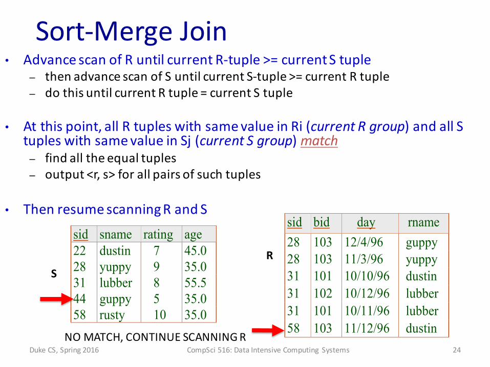
Sort-‐Merge Join
sid sname rating age22 dustin 7 45.028 yuppy 9 35.031 lubber 8 55.544 guppy 5 35.058 rusty 10 35.0
sid bid day rname28 103 12/4/96 guppy28 103 11/3/96 yuppy31 101 10/10/96 dustin31 102 10/12/96 lubber31 101 10/11/96 lubber58 103 11/12/96 dustin
SR
WRITE ONE OUTPUT TUPLE
• Advance scan of R until current R-‐tuple >= current S tuple– then advance scan of S until current S-‐tuple >= current R tuple– do this until current R tuple = current S tuple
• At this point, all R tuples with same value in Ri (current R group) and all S tuples with same value in Sj (current S group) match– find all the equal tuples– output <r, s> for all pairs of such tuples
• Then resume scanning R and S
25Duke CS, Spring 2016 CompSci 516: Data Intensive Computing Systems

Example of Sort-‐Merge Join
• Cost: O(M log M) + O(N log N) + (M+N)– cost of sorting R + sorting S + merging R, S– The cost of scanning, M+N, could be M*N (suppose single value of join attribute in both R and S)
sid sname rating age22 dustin 7 45.028 yuppy 9 35.031 lubber 8 55.544 guppy 5 35.058 rusty 10 35.0
sid bid day rname28 103 12/4/96 guppy28 103 11/3/96 yuppy31 101 10/10/96 dustin31 102 10/12/96 lubber31 101 10/11/96 lubber58 103 11/12/96 dustin
26Duke CS, Spring 2016 CompSci 516: Data Intensive Computing Systems

Cost of Sort-‐Merge Join
• 100 buffer pages• Sort R:
– (pass 0) 1000/100 = 10 sorted runs– (pass 1) merge 10 runs– read + write, 2 passes– 4 * 1000 = 4000 I/O
• Similarly, Sort S: 4 * 500 = 2000 I/O• Second merge phase of sort-‐merge join
– another 1000 + 500 = 1500 I/O• Total 7500 I/O
sid sname rating age22 dustin 7 45.028 yuppy 9 35.031 lubber 8 55.544 guppy 5 35.058 rusty 10 35.0
sid bid day rname28 103 12/4/96 guppy28 103 11/3/96 yuppy31 101 10/10/96 dustin31 102 10/12/96 lubber31 101 10/11/96 lubber58 103 11/12/96 dustin
M = 1000 pages in RpR = 100 tuples per page
N = 500 pages in SpS = 80 tuples per page
• Check yourself:– Consider #buffer
pages 35, 100, 300– Cost of sort-‐merge =
7500 in all three– Cost of block nested
15000, 6000, 2500
27Duke CS, Spring 2016 CompSci 516: Data Intensive Computing Systems
Algorithms for Joins
28
3. HASH JOINS
Duke CS, Spring 2016 CompSci 516: Data Intensive Computing Systems
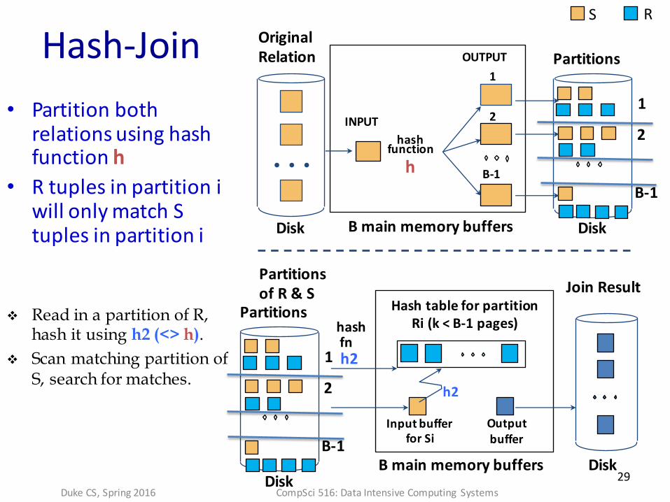
Hash-‐Join• Partition both
relations using hash function h
• R tuples in partition iwill only match S tuples in partition i
v Read in a partition of R, hash it using h2 (<> h).
v Scan matching partition of S, search for matches.
B main memory buffers DiskDisk
Original Relation OUTPUT
2INPUT
1
hashfunctionh B-‐1
Partitions
1
2
B-‐1
. . .
RS
Disk
Partitionsof R & S
Input bufferfor Si
Hash table for partitionRi (k < B-‐1 pages)
B main memory buffers
Output buffer
Disk
Join Result
hashfnh2
h2
Partitions
1
2
B-‐1
Duke%CS,%Spring%2016 CompSci%516:%Data%Intensive%Computing%Systems29

Cost of Hash-‐Join• In partitioning phase
– read+write both relns; 2(M+N)– In matching phase, read both relns; M+N I/Os– remember – we are not counting final write
• In our running example, this is a total of 4500 I/Os– 3 * (1000 + 500)– Compare with the previous joins
• Sort-‐Merge Join vs. Hash Join:– Both can have a cost of 3(M+N) I/Os
• if sort-‐merge gets enough buffer (see 14.4.2)– Hash join holds smaller relation in buffer-‐ better if limited buffer– Hash Join shown to be highly parallelizable– Sort-‐Merge less sensitive to data skew
• also result is sorted.
30Duke CS, Spring 2016 CompSci 516: Data Intensive Computing Systems

General Join Conditions
• Equalities over several attributes– e.g., R.sid=S.sid AND R.rname=S.sname– For Index Nested Loop, build index on <sid, sname> (if S is inner); or use existing indexes on sid or sname.
– For Sort-‐Merge and Hash Join, sort/partition on combination of the two join columns.
• Inequality conditions– e.g., R.rname < S.sname– For Index NL, need (clustered) B+ tree index.– Hash Join, Sort Merge Join not applicable
31Duke CS, Spring 2016 CompSci 516: Data Intensive Computing Systems

Review: Join Algorithms
• Nested loop join: – for all tuples in R.. for all tuples in S….– variations: block-‐nested, index-‐nested
• Sort-‐merge join– like external merge sort
• Hash join
• Make sure you understand how the I/O varies• No one join algorithm is uniformly superior to others– depends on relation size, buffer pool size, access methods, skew
32Duke CS, Spring 2016 CompSci 516: Data Intensive Computing Systems
Algorithms for Set Operations
33Duke CS, Spring 2016 CompSci 516: Data Intensive Computing Systems

Set Operations• Intersection and cross-‐product special cases of join.• Union (Distinct) and Except similar; we’ll do union
– very similar to external sort and join algorithms
• Sorting based approach to union:– Sort both relations (on combination of all attributes)– Scan sorted relations and merge them.– Alternative: Merge runs from Pass 0 for both relations
• Hash based approach to union:– Partition R and S using hash function h.– For each S-‐partition, build in-‐memory hash table (using h2), scan corr. R-‐
partition and add tuples to table while discarding duplicates34Duke CS, Spring 2016 CompSci 516: Data Intensive Computing Systems

Algorithms for Aggregate Operations
35Duke CS, Spring 2016 CompSci 516: Data Intensive Computing Systems

Aggregate Operations (AVG, MIN, etc.)• Without grouping:
– In general, requires scanning the relation.– Given index whose search key includes all attributes in the SELECT or WHERE clauses, can do index-‐only scan
• With grouping:– Sort on group-‐by attributes– or, hash on group-‐by attributes– can combine sort/hash and aggregate– can do index-‐only scan here as well
36Duke CS, Spring 2016 CompSci 516: Data Intensive Computing Systems

Impact of Buffering
• If several operations are executing concurrently, estimating the number of available buffer pages is guesswork.
• Repeated access patterns interact with buffer replacement policy– recall sequential flooding (lecture 6 and piazza post)– e.g., Inner relation is scanned repeatedly in Simple Nested Loop Join– With enough buffer pages to hold inner, replacement policy does
not matter– Otherwise, MRU is best, LRU is worst
37Duke CS, Spring 2016 CompSci 516: Data Intensive Computing Systems

Summary
• A virtue of relational DBMSs: queries are composed of a few basic operators– the implementation of these operators can be carefully tuned (and it is important to do this!).
• Many alternative implementation techniques for each operator– no universally superior technique for most operators.
• Must consider available alternatives for each operation in a query and choose best one based on system statistics, etc.– This is part of the broader task of optimizing a query composed of several ops.
38Duke CS, Spring 2016 CompSci 516: Data Intensive Computing Systems
Query Optimization
39Duke CS, Spring 2016 CompSci 516: Data Intensive Computing Systems
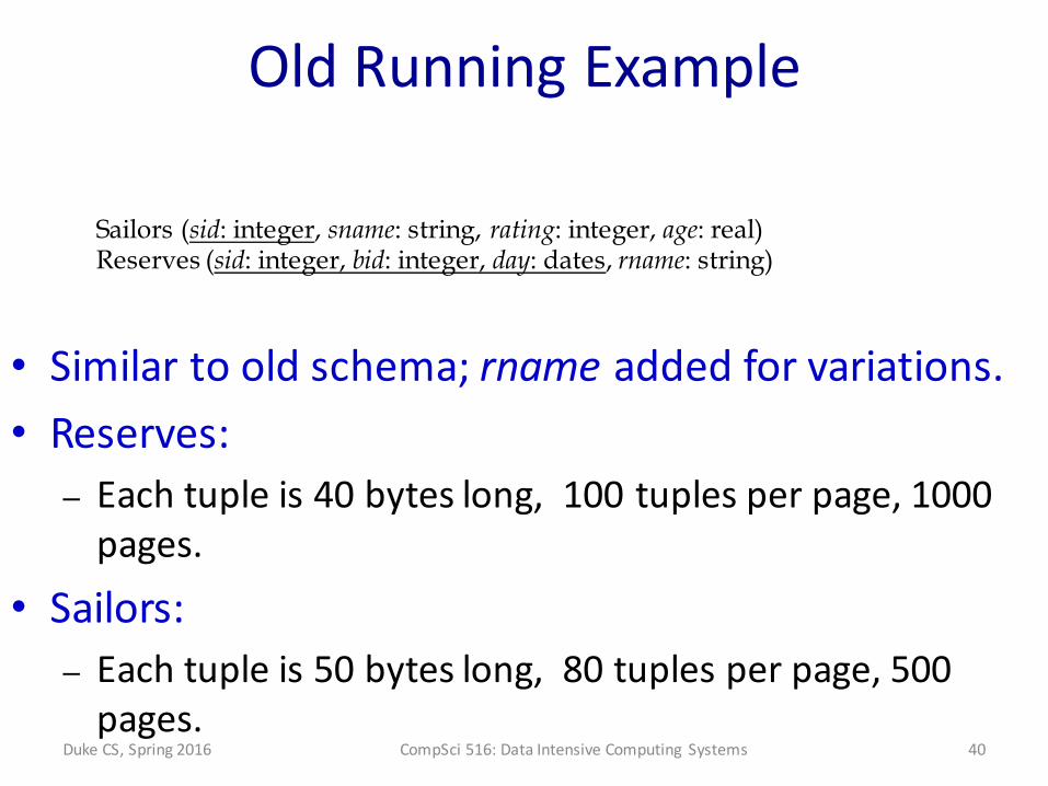
Old Running Example
• Similar to old schema; rname added for variations.• Reserves:
– Each tuple is 40 bytes long, 100 tuples per page, 1000 pages.
• Sailors:– Each tuple is 50 bytes long, 80 tuples per page, 500 pages.
Sailors (sid: integer, sname: string, rating: integer, age: real)Reserves (sid: integer, bid: integer, day: dates, rname: string)
40Duke CS, Spring 2016 CompSci 516: Data Intensive Computing Systems

Query Blocks: Units of Optimization
• Query Block– No nesting– One SELECT., one FROM– At most one WHERE, GROUP BY, HAVING
• SQL query • => parsed into a collection of query blocks• => the blocks are optimized one block at a
time
• First we discuss single query block• Express it as a relational algebra (RA)
expression
SELECT S.snameFROM Sailors SWHERE S.age IN
(SELECT MAX (S2.age)FROM Sailors S2GROUP BY S2.rating)
Nested blockOuter block
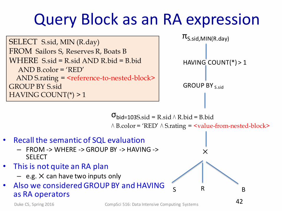
Query Block as an RA expression
• Recall the semantic of SQL evaluation– FROM -‐> WHERE -‐> GROUP BY -‐> HAVING -‐>
SELECT• This is not quite an RA plan
– e.g. ⨉ can have two inputs only• Also we considered GROUP BY and HAVING
as RA operators
SELECT S.sid, MIN (R.day)FROM Sailors S, Reserves R, Boats BWHERE S.sid = R.sid AND R.bid = B.bid
AND B.color = ‘RED’ AND S.rating = <reference-to-nested-block>
GROUP BY S.sidHAVING COUNT(*) > 1
S R
σbid=103S.sid = R.sid ⋀ R.bid = B.bid⋀ B.color = ‘RED’ ⋀ S.rating = <value-from-nested-block>
πS.sid,MIN(R.day)
B
⨉
GROUP BY S.sid
HAVING COUNT(*) > 1
Duke%CS,%Spring%2016 CompSci%516:%Data%Intensive%Computing%Systems 42
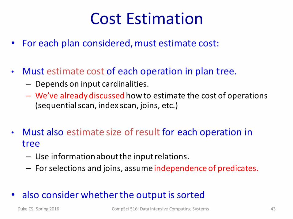
Cost Estimation• For each plan considered, must estimate cost:
• Must estimate cost of each operation in plan tree.– Depends on input cardinalities.– We’ve already discussed how to estimate the cost of operations
(sequential scan, index scan, joins, etc.)
• Must also estimate size of result for each operation in tree– Use information about the input relations.– For selections and joins, assume independence of predicates.
• also consider whether the output is sorted43Duke CS, Spring 2016 CompSci 516: Data Intensive Computing Systems

Estimating Result Sizes
• Max #tuples = – |R1|⨉ |R2| ⨉ |R3| ⨉ ….
• But we can model the effect of WHERE clause by associating a reduction factor for each <condn>
SELECT <attr>FROM R1, R2, R3, ….WHERE <condn1> AND
<condn2>..
44Duke CS, Spring 2016 CompSci 516: Data Intensive Computing Systems
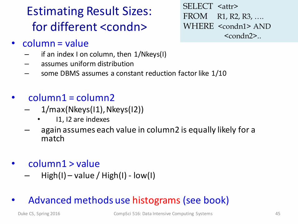
Estimating Result Sizes: for different <condn>
• column = value– if an index I on column, then 1/Nkeys(I)– assumes uniform distribution– some DBMS assumes a constant reduction factor like 1/10
• column1 = column2– 1/max(Nkeys(I1), Nkeys(I2))
• I1, I2 are indexes– again assumes each value in column2 is equally likely for a
match
• column1 > value– High(I) – value / High(I) -‐ low(I)
• Advanced methods use histograms (see book)
SELECT <attr>FROM R1, R2, R3, ….WHERE <condn1> AND
<condn2>..
45Duke CS, Spring 2016 CompSci 516: Data Intensive Computing Systems
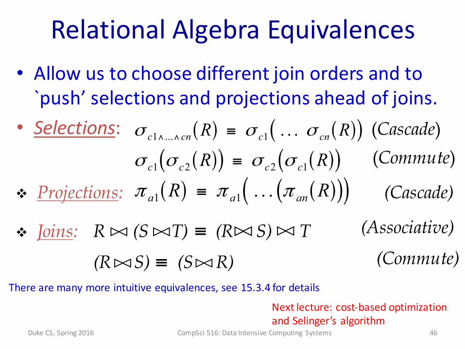
Relational Algebra Equivalences• Allow us to choose different join orders and to `push’ selections and projections ahead of joins.
• Selections: ( ) ( )( )σ σ σc cn c cnR R1 1∧ ∧ ≡... . . .
( )( ) ( )( )σ σ σ σc c c cR R1 2 2 1≡ (Commute)
v Projections: ( ) ( )( )( )π π πa a anR R1 1≡ . . . (Cascade)
v Joins: !"R (S T) (R S) T!" !" !"≡ (Associative)
!"(R S) (S R) !" ≡ (Commute)
(Cascade)
There are many more intuitive equivalences, see 15.3.4 for details
Next lecture: cost-‐based optimization and Selinger’s algorithm
46Duke CS, Spring 2016 CompSci 516: Data Intensive Computing Systems


