
Complete Path Planning for Planar Closed Chains Among Point Obstacles
Guanfeng Liu and Jeff Trinkle
Rensselaer Polytechnic Institute
Outline: Motivation and overview C-space Analysis
Number of components C-space topology Local parametrization and global atlas
Boundary variety Global cell decomposition Path Planning algorithm Simulation results
Motivation:
Many applications employ closed-chain manipulators
No complete algorithms for closed chains with obstacles
Limitation of PRM method for closed chains
Difficulty to apply Canny’s roadmap method to C-spaces with multiple coordinate charts
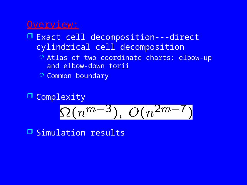
Overview: Exact cell decomposition---direct cylindrical
cell decomposition Atlas of two coordinate charts: elbow-up and
elbow-down torii Common boundary
Complexity
Simulation results

C-space Analysis Dimension: m-3 for m-link closed chains Algebraic variety Number of components
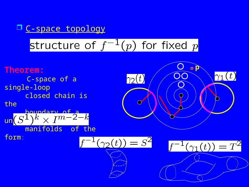
Theorem: C-space of a single-loop closed chain is the boundary of a union of manifolds of the form:
C-space topology
p
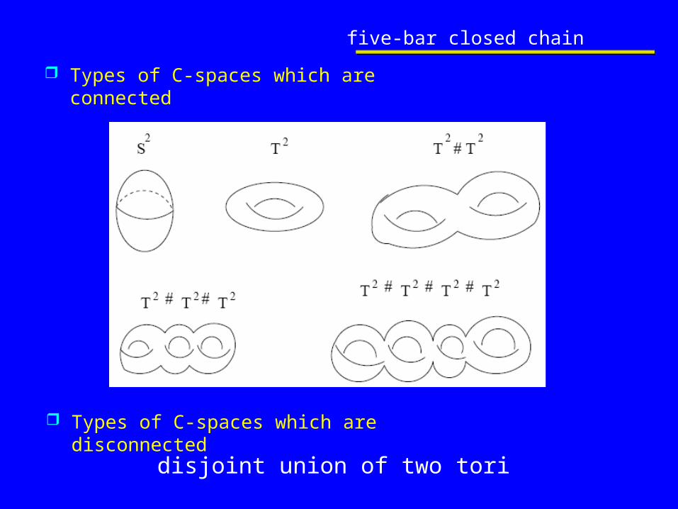
five-bar closed chain
Types of C-spaces which are connected
Types of C-spaces which are disconnected
disjoint union of two tori

Local and global parametrization
Any m-3 joints can be used as a local chart
More than two charts for differentiable covering Example: 2n charts required to cover (S1)n
Two charts (elbow-up and elbow-down) for capturing
connectivity
1
2
3
4
5
l1
l2
l3
l4 l5
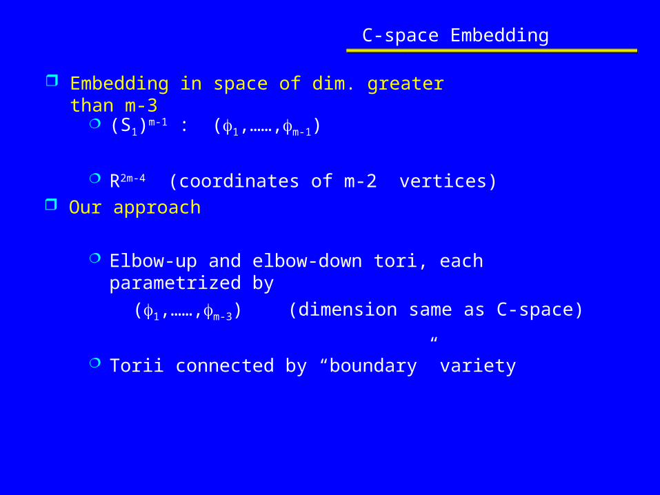
C-space Embedding
(S1)m-1 : (1,……,m-1)
R2m-4 (coordinates of m-2 vertices)
Elbow-up and elbow-down tori, each parametrized by
(1,……,m-3) (dimension same as C-space)
Torii connected by “boundary” variety
Embedding in space of dim. greater than m-3
Our approach
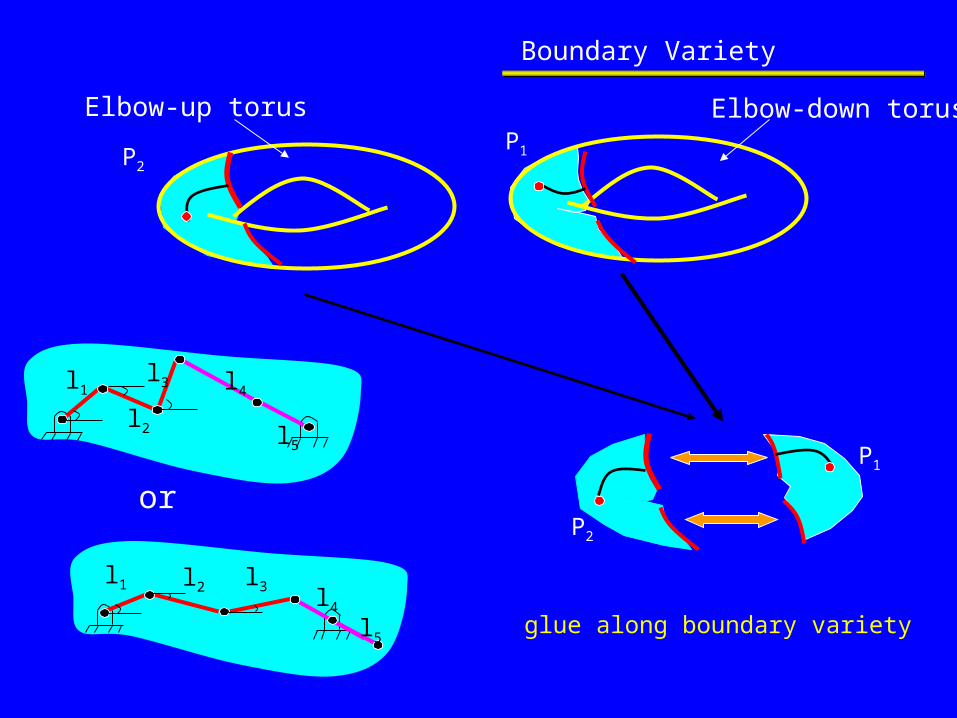
Boundary Variety
glue along boundary variety
P1
P2
l1l2
l3 l4
l5
or
l1 l2 l3l4
l5
Elbow-up torus Elbow-down torusP1P2

Main steps
Boundary variety and its recursive skeletons Collision varieties
Cell decomposition for elbow-up and elbow-down torii
Identify valid cells based on boundary variety
Adjacency between cells in elbow-up and elbow-down torii
Global graph representation
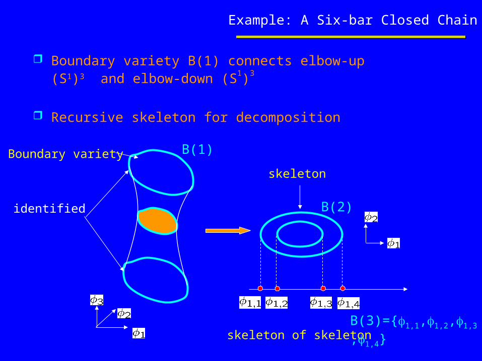
Example: A Six-bar Closed Chain
Boundary variety B(1) connects elbow-up (S1)3 and elbow-down (S1)3
Recursive skeleton for decomposition
Boundary variety
skeleton
skeleton of skeleton
B(1)
B(2)
B(3)={1,1,1,2,1,3,
1,4}
identified

Geometric interpretation
1
2 3l1
l2
l3 l4
l5
l2l1
l3 l4 l5 l1l3 l4 l5
l2
l1
Boundary variety
skeleton
Skeleton of skeleton
B(1)
B(2)
B(3)

Cell decomposition and graph representation
Elbow-up torus Elbow-down torus

graph representation
Elbow-up torus Elbow-down torus
[B1(1),1]
[1,2]
[2,B2(1)]
[B1(1),2]
[2,B2(1)]
[B1(1),1]
[1,2]
[2,B2(1)]
[B1(1),2]
[2,B2(1)]
Common facets on B(1)
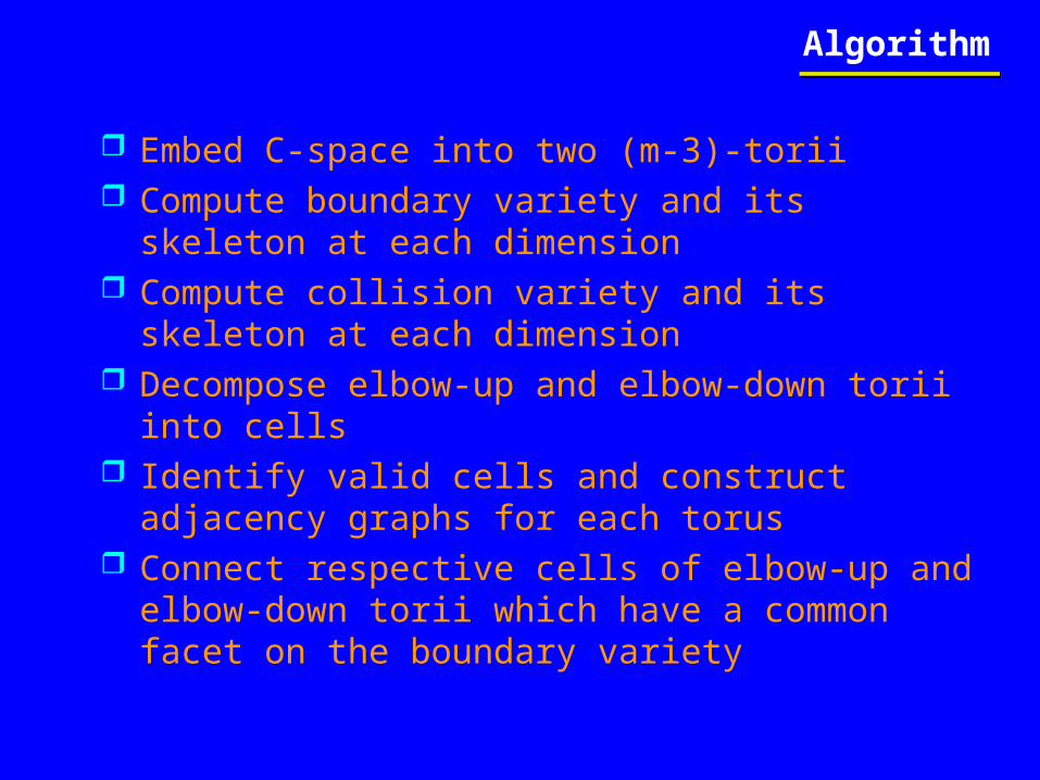
Embed C-space into two (m-3)-torii Compute boundary variety and its skeleton at
each dimension Compute collision variety and its skeleton at
each dimension Decompose elbow-up and elbow-down torii into
cells Identify valid cells and construct adjacency
graphs for each torus Connect respective cells of elbow-up and elbow-
down torii which have a common facet on the boundary variety
Algorithm

Video
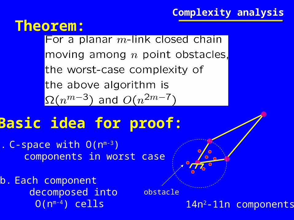
Complexity analysis
Theorem:
Basic idea for proof:a. C-space with O(nm-3) components in worst case
b. Each component decomposed into O(nm-4) cells
obstacle
14n2-11n components
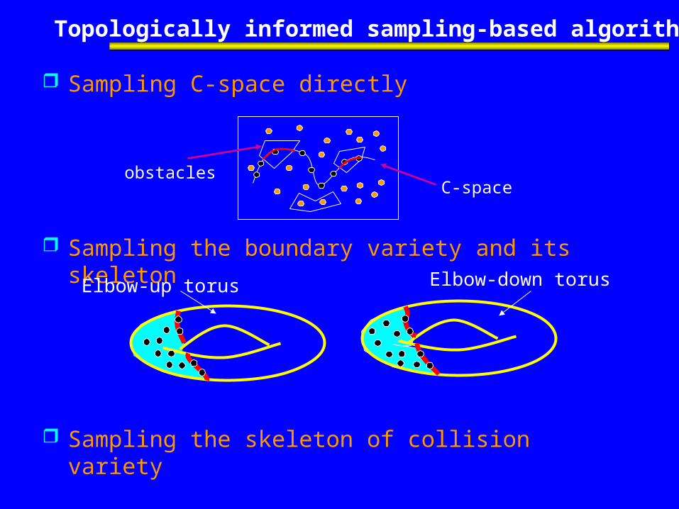
Topologically informed sampling-based algorithms
Sampling C-space directly
Sampling the boundary variety and its skeleton
Sampling the skeleton of collision variety
C-spaceobstacles
Elbow-down torusElbow-up torus
Summary
Global structure of C-space
Atlas with two coordinate charts
Boundary variety and its skeleton
Cell-decomposition algorithm
Topologically informed sampling-based algorithms


