Comparisons of laboratory scale measurementsof three-dimensional acoustic propagation withsolutions by a parabolic equation model
Fr�ed�eric Sturma) and Alexios KorakasLaboratoire de M�ecanique des Fluides et d’Acoustique—Unit�e Mixte de Recherche, Centre National de laRecherche Scientifique 5509 ECL-UCBL1-INSA de Lyon, Ecole Centrale de Lyon, F-69134 Ecully Cedex,France
(Received 25 June 2012; revised 16 October 2012; accepted 20 November 2012)
In this paper, laboratory scale measurements of long range across-slope acoustic propagation in a
three-dimensional (3-D) wedge-like environment are compared to numerical solutions. In a previ-
ous work, it was shown that the experimental data contain strong 3-D effects like mode shadow
zones and multiple mode arrivals, in qualitative agreement with theoretical and numerical predic-
tions. In the present work, the experimental data are compared with numerical solutions obtained
using a fully 3-D parabolic equation based model. A subspace inversion approach is used for the
refinement of some of the parameters describing the model experiment. The inversion procedure is
implemented in a Bayesian framework based on the exhaustive search over the parameter space.
The comparisons are performed both in the time and in the frequency domain using the maximum aposteriori estimates of the refined parameters as input in the 3-D model. A very good quantitative
agreement is achieved between the numerical predictions provided by the 3-D parabolic equation
model and the experimental data. VC 2013 Acoustical Society of America.
[http://dx.doi.org/10.1121/1.4770252]
PACS number(s): 43.30.Zk, 43.30.Dr, 43.30.Bp, 43.30.Gv [TD] Pages: 108–118
I. INTRODUCTION
The study of 3-D acoustic propagation in realistic oce-
anic environments has received a lot of attention during the
last three decades (see, for instance, Ref. 1, and references
therein). More recently, renewed interested stimulated by ex-
perimental evidence of 3-D propagation2–6 has given rise to
an increasing number of publications reporting develop-
ments in theoretical and numerical 3-D modeling.7–13 Of
particular importance is the establishment of test cases for
3-D model validation and performance comparison. Signifi-
cant efforts have been put into establishing benchmark solu-
tions to canonical test cases,14 among which notable is the
3-D ASA wedge problem simulating a continental shelf
environment. However, unlike in 2-D propagation prob-
lems,15,16 experimental measurements of 3-D propagation
having the potential of being established as real-data bench-
marks are rare in the literature.
In this context, two laboratory-scale experimental cam-
paigns were led in 2006 and 2007 in the large indoor tank of
the LMA-CNRS laboratory in Marseille, aimed at collecting
3-D acoustic propagation data over a tilted bottom in a well-
controlled environment. The first campaign mainly consisted
of preliminary tests, whereas the second was intended to col-
lect high quality data. Operational frequencies and water
depths were chosen to produce a reduced number of modes
in order to facilitate the analysis of modal propagation in the
wedge-like waveguide. In both campaigns, the experimental
data exhibited prominent 3-D propagation effects like multi-
ple mode arrivals, mode shadow zones, intra-mode interfer-
ence and focusing, all consistent with well-known 3-D
effects described in the literature.1,17,18 In addition, the data
were in good qualitative agreement with both time- and
frequency-domain simulations by a 3-D parabolic equation
(PE)-based code19 using the measured parameter values
from the tank. Yet, quantitative comparisons turned out to be
hindered by the uncertainties associated with some parame-
ters, being large with respect to their potential impact on the
acoustic field. Besides, improving the comparisons by blind
testing of different sets of parameter values within their mar-
gins of uncertainty is a highly time-consuming task when
comparing to 3-D model solutions.
In this paper, numerical results by a 3-D PE model are
reported and compared to the 3-D propagation data collected
during the second campaign. The parameter values used in
the 3-D PE marching algorithm yielding the best match with
the data are obtained using a subspace inversion approach
based on the 3-D PE model. The present paper is organized
as follows. The experimental set-up is recalled in Sec. II.
The inversion procedure, implemented in a Bayesian frame-
work, is detailed in Sec. III. Comparisons between experi-
mental and numerical results are presented in Sec. IV both in
the time and in the frequency domain. The paper closes with
some concluding remarks. Preliminary results of the present
work were presented during the 4th International Conference
& Exhibition on Underwater Acoustic Measurements held in
Kos, Greece in 2011.
II. LABORATORY SCALE MEASUREMENTS
The scaled experiments presented here and considered
in the remainder of this paper were conducted in July 2007
a)Author to whom correspondence should be addressed. Electronic mail:
108 J. Acoust. Soc. Am. 133 (1), January 2013 0001-4966/2013/133(1)/108/11/$30.00 VC 2013 Acoustical Society of America
Downloaded 01 Mar 2013 to 128.197.27.9. Redistribution subject to ASA license or copyright; see http://asadl.org/terms

at the indoor shallow-water tank of the LMA-CNRS labora-
tory in Marseille. The inner tank dimensions are 10-m-long,
3-m-wide, and 1-m-deep. As illustrated in Fig. 1, a thin layer
of water overlies a thick layer of calibrated river sand simu-
lating a bottom half-space. A sloping bottom geometry with
the wedge apex oriented lengthwise over the entire length of
the tank was produced using a rake inclined at 4.5� (visible
in the background of Fig. 1). The water depth at the source
was measured using a separate high-frequency transducer
(not shown here) yielding 48 mm, though one may expect an
error of about 10%. Indeed, an overestimate of approxi-
mately 1 mm was attributed to surface tension effects in the
very near vicinity of the transducer, whereas non-negligible
evaporation relative to the water depth was observed during
the measurements. The sound speed in the bottom was meas-
ured on sand samples to avoid damaging the bottom geome-
try, leading to 1660 m/s. However, during the calibration
phase over a flat bottom,20 it appeared more reasonable to
consider a value within (1700 6 50) m/s due to an apparently
different consolidation of the sand in the tank. The density
of the sandy bottom was measured to be (1.99 6 0.01)
g/cm3. The value of the bottom sound attenuation could not
be measured at the central frequency (150 kHz) considered in
the tank experiment (see discussion hereafter). The value of
(0.5 6 0.1) dB per wavelength attributed to the attenuation at
150 kHz was extrapolated from attenuation values measured at
higher frequencies. It is to be noticed that this value is a typical
value for the specific type of sediment used. Most important is
that this specific value permitted successful comparisons
between theory and experiment during the calibration phase
(see Ref. 20).
The source and receiver, illustrated in Fig. 1, were pie-
zoelectric transducers having cylindrical shapes with 6-mm
external diameter. Prior to the measurements, the signal used
for transmission at the source was analyzed in a deep-water
tank in order to avoid unwanted echoes. The signal recorded
at 68 mm from the source is shown in the left panel of Fig. 2
where it appears well separated in time from its echoes (top
left panel). It is a five-cycle pulse with Gaussian envelope
with 0.04 ms duration and with a weak tail of approximately
the same duration due to the mechanical response of the
transducer. Its frequency spectrum (right panel of Fig. 2)
presents a main lobe centered at 150 kHz with a 100 kHz
bandwidth as well as a secondary lobe above 200 kHz attrib-
uted to the distortion in the time signal observed at 0.03 ms
(bottom left panel of Fig. 2). Note here that a 2-D normal
mode code predicts that four trapped modes are excited at
the source for the frequency of 150 kHz. During the meas-
urements in the shallow-water tank, the source was kept at a
fixed position and the receiver was moved within a vertical
plane in the across-slope direction (parallel to the wedge
apex). The received time signals were recorded in a time
window of 5 ms at a rate of 10 MHz and averaged over five
repeated measurements. An embankment of sand along the
side-walls on the deep-water side of the tank achieved signif-
icant attenuation of the unwanted reflections in the recorded
signals. Note, however, that the use of short pulses for trans-
mission allows discarding the unwanted reflections by appro-
priate choice of a truncation window.
The focus in this paper is on two main data sets that
were collected during two different days in a same week.
The first data set provided fine sampling of the sound field in
range and is herein referred to as ASP-H (for horizontal
measurements of across-slope propagation). This data set
consists of time signals recorded at a fixed receiver depth
and at several source/receiver separations ranging from
r¼ 0.1 m to r¼ 5 m in increments of 0.005 m. The measure-
ments were repeated for three distinct source depths (SD),
namely, 10 mm (all modes excited), 19 mm (mode 3 weakly
excited), and 26.9 mm (modes 2 and 4 weakly excited), giv-
ing rise to three distinct data subsets herein referred to as
ASP-H1, ASP-H2, and ASP-H3, respectively. The second
data set provided fine sampling of the sound field in depth, at
several coarser source/receiver separations and is herein
referred to as ASP-V (for vertical measurements of across-
slope propagation). The time signals in this data set were
recorded at consecutive ranges from the source in 0.1 m
increments where at each range they were recorded at sev-
eral receiver depths from zR¼ 1 mm to zR¼ 44 mm in incre-
ments of 1 mm. The water sound speed was deduced from
the temperature of the water,21 which was 21.95� (respec-
tively, 22.13�) during the ASP-H1 measurements (respec-
tively, ASP-H2 and ASP-H3), thus leading to a water sound
speed of 1488.15 m/s (respectively, 1488.7 m/s), and 22.19�
during the ASP-V measurements leading to 1488.9 m/s.
FIG. 1. (Color online) View of the shallow water tank (facilities of the
LMA-CNRS laboratory) used in the experimental campaign, showing the
source and the receiver both aligned along the across-slope direction of the
wedge-shaped waveguide. The rake that was used to tilt the sandy bottom
with a sloping angle of � 4.5� can be seen on the background.
FIG. 2. Source signal (left) and its spectrum (right).
J. Acoust. Soc. Am., Vol. 133, No. 1, January 2013 F. Sturm and A. Korakas: Comparisons of laboratory scale measurements 109
Downloaded 01 Mar 2013 to 128.197.27.9. Redistribution subject to ASA license or copyright; see http://asadl.org/terms

Figure 3 shows stacked time series versus range in the
across-slope direction as recorded, from left to right, during
the ASP-H1, ASP-H2, and ASP-H3 measurements respec-
tively. The time series have been scaled appropriately to
compensate for cylindrical spreading.
Overall, four modes can be identified by inspection of
the depth stacks from the ASP-V data set (not shown here,
see Ref. 22), denoted M1, M2, M3, and M4, respectively.
The range stacks in Fig. 3 exhibit multiple mode arrivals,
mode shadow zones, and intra-mode interference, which are
typical 3-D effects identical to those described in the litera-
ture for the wedge-like environment.17,18 For instance, at
some range, mode 2 (denoted M2) presents two distinct
arrivals that progressively overlap (i.e., interfere) as the
receiver moves out in range across-slope, and eventually
reaches its cut-off range beyond which its shadow zone
extends. For a detailed description of the 3-D effects
observed in the measurements, the reader is referred to Ref.
22. We note here the effect of the source depth being in the
vicinity of a node of mode 3 in Fig. 3(b), and in the vicinity
of the nodes of mode 2 and 4 in Fig. 3(c).
Let us conclude this section with two observations. First
of all, in Fig. 3(a), we observe a slight unexpected delay in
the arrival times of the recorded signals beyond the range of
3.5 m, which becomes significant beyond the range of 4.5 m.
This delay, which is clearly not present in the ASP-H2 and
ASP-H3 data sets, is likely due to a malfunction of the step-
ping mechanism moving the receiver during the ASP-H1
measurement. Finally, it is to be noticed that the noise-like
signals observed, e.g., between the two arrivals of mode 1
beyond the range of 4 m in Fig. 3, pertain to the secondary
lobe of the frequency spectrum in Fig. 2. These two issues
will be further discussed in Sec. IV where the data are com-
pared to numerical simulations.
III. REFINEMENT OF MODEL PARAMETERS
A first, although encouraging, comparison of broadband
predictions provided by a 3-D parabolic equation based code
using the measured parameter values from the model experi-
ment suggested a refinement was required. A simple inver-
sion procedure is thus used to provide estimates of the
parameters affecting propagation.
A. Inversion approach
The inversion is implemented in a Bayesian framework
following the derivation by Refs. 23 and 24. In the Bayesian
formulation, the solution to the inverse problem is fully char-
acterized by the posterior probability density (PPD) of the
parameters. Let the N-length complex vector dl denote the
spectral components of the observed data recorded on a
N-element receiving array at frequency fl, and the M-length
vector m denote the parameters to be recovered. The PPD,
defined as the probability density function (pdf) of m given
dl, is written as
pðm j dlÞ ¼LðmÞpðmÞð
MLðm0Þpðm0Þdm0
; (1)
FIG. 3. Experimental signals extracted from the ASP-H data set. Stacked time series versus source/receiver range corresponding to the experimental data
recorded along the across-slope direction for a source depth of (a) 10 mm (ASP-H1 data; all modes are excited), (b) 19 mm (ASP-H2 data; mode 3 is weakly
excited), (c) 26.9 mm (ASP-H3 data; both modes 2 and 4 are weakly excited). For each panel, the receiver depth is 10 mm.
110 J. Acoust. Soc. Am., Vol. 133, No. 1, January 2013 F. Sturm and A. Korakas: Comparisons of laboratory scale measurements
Downloaded 01 Mar 2013 to 128.197.27.9. Redistribution subject to ASA license or copyright; see http://asadl.org/terms
where L(m) is the likelihood function, p(m) is the prior pdf
reflecting a priori knowledge on the parameters, and the
integration in the denominator is taken over the whole pa-
rameter space M. The likelihood function gives a measure
of fit between the observed data vector and the replica vector
wl(m) provided by an ocean acoustic propagation model. It
takes various forms depending on the amount of the data
exploited in the inversion.25 Likelihood functions used in
this paper are derived under the assumption of additive com-
plex Gaussian distributed errors. They are given in the Ap-
pendix and the reader is referred to Ref. 25 for a detailed
discussion. For the purpose of this work, the PPD is sampled
over the parameter space using exhaustive search, also
known as a grid search.23,26 This requires defining bounds
for each parameter and discretizing the resulting search
intervals. In practice, a replica vector is generated for each
combination of the discrete values of the parameters and the
major part of the central processing unit (CPU) time is spent
on this task alone. A convenient estimate of m for experi-
ment-versus-theory comparisons is the maximum a posteri-ori (MAP) estimate obtained by maximizing the PPD. The
posterior mean estimate and standard deviation, along with
the posterior marginal densities, can be used to assess the
quality and dispersion of the estimate.
B. Parameterization
The assumptions on the environmental model adopted
for replica generation are similar to those of the synthetic
3-D ASA wedge benchmark (see, e.g., Ref. 27), i.e., a water
layer of constant sound speed lying over a fluid bottom half-
space with constant parameters (sound speed, density, and
sound attenuation), and a water/bottom interface presenting
a constant slope. Point source and receivers are considered
and the vertical plane containing them, referred to as the ob-
servation plane, is oriented in the across-slope direction (i.e.,
perpendicular to the slope) along which the water depth is
constant and equal to the water depth at the source.
The parameters that are to be refined are those that can
significantly affect the acoustic field within their margins of
uncertainty. In the actual experimental context and for the
considered operational frequencies, these are the water
depth, the source and receiver depths, the slope, and the bot-
tom parameters. Indeed, as discussed in Sec. II, the measured
value of the water depth, denoted hS, appeared to be overesti-
mated and has thus to be included in the parameterization of
the inverse problem. Because of the large dimension of the
transmitting and receiving transducers relative to the water
depth, the source and receiver depths, respectively, denoted zS
and zR, are also included in the parameterization in order to
obtain equivalent point source and receiver depths that provide
the best match between experiment and theory. Furthermore,
the sloping geometry of the sandy bottom was created using a
rake inclined at 4.5� thus resulting in a slope of approximately
the same value. It is also included in the parameterization in
an effort to obtain a more accurate estimate.
Finally, although the assumption of a fluid bottom half-
space with constant parameters might not exactly reflect reality
at the considered frequencies, it yielded excellent comparisons
between experiment and theory during the calibration phase
over a flat bottom.20 In particular, the values of 1.99 g/cm3 and
0.5 dB per wavelength were used, respectively, for the bottom
density and the sound attenuation in the bottom (see discussion
in Sec. II), whereas a reasonable value for the bottom sound
speed appeared to be 1700 m/s. We anticipate that inverting for
an equivalent constant bottom sound speed yields estimates
that are not well resolved, resulting in to values that appear to
be frequency and/or range dependent. The bottom parameters
are thus kept fixed during the inversion at their respective val-
ues mentioned above. The parameterization of the inverse
problem can thus be expressed as m¼ [hS, zS, zR, slope]T. Other
parameters involved in the environmental model are kept fixed
at their nominal values during the inversion.
C. Inversion setup
At first glance, the prominent 3-D effects observed in
the recorded time signals suggest that the use of fully 3-D
computations is necessary for replica generation. However,
an inversion based on 3-D computations quickly becomes
impractical for more than two parameters at a time due to
the dramatically increased CPU times. This is true even with
the use of more elaborate and efficient sampling algorithms
than exhaustive search. In a recent work, it was shown that
the slope effect onto inversions of simulated vertical array
data in a 3-D wedge test case can be neglected at relatively
short ranges from the source.28 In other words, an inversion
based on a 2-D model succeeds in retrieving the correct
parameter values at short ranges. Applying this observation
to the actual experimental context suggests that an inversion
of vertical array data be performed in two steps as follows.
Step 1: inversion of short range vertical array data based
on 2-D computations for the refinement of the so-called geo-
metrical parameters, i.e., the water depth, the source depth,
and the receiver depths, which are known to be dominant
close to the source.
Step 2: inversion of vertical array data at farther ranges,
where propagation is strongly affected by 3-D effects, for the
recovery of the slope while keeping the geometrical parame-
ters fixed at their MAP estimates deduced from the first step.
It is understood that the second inversion step requires
3-D computations for replica generation. Furthermore, it was
shown that the objective function is highly sensitive to the
slope whenever the array is positioned in the vicinity of the
caustic or cut-off range of a single mode.28 This observation
is useful for choosing appropriate vertical array ranges in the
second step. The two-step inversion approach can thus be
applied on the ASP-V data set (described in Sec. II) where,
for a given range, the consecutive fine measurements in
depth can be viewed as measurements on a synthetic vertical
array. When it comes to comparisons with ASP-H1, ASP-
H2, and ASP-H3 data sets, new inversions are required in
order to refine the geometrical parameters that are expected
to be slightly different due to evaporation and subsequent
refilling of the tank with fresh water. Here, for given source
and receiver depths, the consecutive fine measurements in
range are viewed as measurements on a synthetic horizontal
array. Note now that the relative phase along a horizontal
J. Acoust. Soc. Am., Vol. 133, No. 1, January 2013 F. Sturm and A. Korakas: Comparisons of laboratory scale measurements 111
Downloaded 01 Mar 2013 to 128.197.27.9. Redistribution subject to ASA license or copyright; see http://asadl.org/terms

array is sensitive to the 3-D variability of the acoustic field,
even at short ranges. Therefore, the inversion of the ASP-H
data set require replica generated by 3-D computations,
which will now be using the MAP estimate of the slope from
the two-step inversion. The choice of appropriate array posi-
tion and aperture is thus constrained by the increased CPU
times needed for a 3-D-model-based inversion.
D. Inversion results
The observed data vector dl is composed of spectral
components of the 4096-point windowed and Fourier-
transformed time signals recorded at consecutive receiver
positions forming a synthetic array. In each inversion five
frequency bins are used: 131.8, 141.6, 151.3, 161.1, and
170.8 kHz. For each frequency, the replica vector wl(m) is
generated at a scale of 1000:1 using the parabolic equation
based code 3DWAPE (Ref. 29) for both 2-D and 3-D computa-
tions. The prior pdf p(m) is chosen uniform within the
search intervals of each parameter (as given in the abscissa
of Figs. 4 and 5) and zero elsewhere. The discretization is
sufficiently fine to ensure convergence.
1. Two-step inversion of ASP-V data set
In both steps of ASP-V data inversion, a synthetic verti-
cal line array composed of 40 receivers at nominal depths
from 5 to 44 mm with a 1 mm depth increment is used. In the
first inversion step the separation from the source is 0.1 m,
whereas the ranges for the second step are chosen in the vi-
cinity of mode-2 caustic occurring, for each respective fre-
quency, at 2.6, 2.8, 2.9, 3.1, and 3.2 m from the source.
The PPD in Eq. (1) is evaluated using the likelihood
function defined in Eq. (A3) which is equivalent to correlat-
ing observed and predicted complex acoustic field vectors.
Recall that the first step is based on 2-D computations,
whereas the second step requires 3-D computations. Accord-
ingly, the single-processor CPU time for a single-frequency
inversion is approximately 5 min in the first step (requiring
1891 replica vector generation), whereas it ranges from 3 to
5 h in the second step (requiring 25 replica vector generation).
Figure 4 shows posterior marginal densities of the refined
parameters in the first [Fig. 4(a)] and second [Fig. 4(b)]
inversion steps. The resulting estimates are summarized in
Table I. Overall, the marginal densities present narrow con-
centrations around the mean estimates and are relatively sym-
metric so that the means coincide with the MAP estimates.
Note the steep peak in Fig. 4(b) as a result of the importance
of the slope in the vicinity of the mode-2 caustic.
2. Inversion of ASP-H data set
A synthetic horizontal line array is used here, composed
of 16 receivers at nominal ranges from 0.15 to 0.3 m with a
0.01 m range increment and at a nominal depth of 10 mm.
The PPD is now evaluated using the likelihood function
defined in Eq. (A7) which is equivalent to fitting the trans-
mission loss curves along the horizontal array. The inversion
is repeated for each of the ASP-H1, ASP-H2, and ASP-H3
data sets, recalling that they were obtained for three distinct
nominal source depths at 10, 19, and 26.9 mm, respectively.
The inversion of horizontal data, requiring 3-D computa-
tions, resulted in 4 to 6 h CPU times for a single frequency.
Figure 5 shows posterior marginal densities of the refined
parameters for each of the three inversions, with resulting
estimates given in Table I. Overall, similar observations apply
here except for the notable multimodal character of the mar-
ginals of the source depth and the receiver depth offset in the
ASP-H1 inversion. The two-dimensional posterior marginal
density for these two parameters (not shown here) reveals a
strong negative correlation, suggesting that, although the
MAP estimate strictly results in (zS, dzR)¼ (8.30,� 0.7) mm,
the choice (zS, dzR)¼ (9.30, �1.7) mm is also acceptable. In
other words, we expect that positioning the source 1-mm
deeper and the receiving array 1-mm shallower yields a simi-
lar quality of fit between experimental and simulated transmis-
sion loss curves. We note that in this case the mean estimate
has no meaning as it only gives the average of the two peaks.
Note finally the decrease in the estimated value of the water
depth from ASP-H1 to ASP-H3 inversion, most probably due
to evaporation during the day the data were collected.
FIG. 4. Posterior marginal densities of (a) the water depth, hS, the source
depth, zS, and the receiving array depth offset, dzR, obtained in the first
inversion step of ASP-V data set, (b) the slope obtained in the second inver-
sion step of ASP-V data set.
FIG. 5. Posterior marginal densities of the water depth, hS, the source depth,
zS, and the receiving array depth offset, dzR, obtained from inversions of (a)
ASP-H1, (b) ASP-H2, and (c) ASP-H3 data sets.
112 J. Acoust. Soc. Am., Vol. 133, No. 1, January 2013 F. Sturm and A. Korakas: Comparisons of laboratory scale measurements
Downloaded 01 Mar 2013 to 128.197.27.9. Redistribution subject to ASA license or copyright; see http://asadl.org/terms
IV. NUMERICAL SIMULATIONS AND COMPARISONS
In this section we compare numerical simulations
obtained using the 3-D parabolic equation based model
3DWAPE (Ref. 29) to the ASP-H1, ASP-H2, and ASP-H3 ex-
perimental data sets. For convenience, in all the simulations,
a scale factor of 1000:1 was used with respect to the experi-
mental configuration. Note that, as in Ref. 15, the scale factor
of 1000:1 was applied in all the simulations, where the fre-
quencies and lengths have been appropriately modified (but
keeping the 0.5 dB per wavelength value for the compres-
sional attenuation coefficient in the fluid bottom layer), to
show the analogy between propagation in the tank and an
oceanic waveguide. The wedge-shaped computational do-
main consists of a lossless homogeneous water layer with the
relevant value of the sound speed (1488.2 m/s for ASP-H1,
and 1488.7 m/s for both ASP-H2 and ASP-H3) and a density
of 1 g/cm3, overlying a lossy half-space sediment bottom
truncated at a depth of 600 m below the seafloor, with a ho-
mogeneous sound speed of 1700 m/s, a density of 1.99 g/cm3,
and a sound attenuation of 0.5 dB per wavelength. For each
comparison, separate runs of the 3-D PE code were per-
formed using the MAP estimates of the geometrical parame-
ters as given in Table I for the respective data set. In all the
comparisons, the slope of the tilted bottom was set equal to
4.55� corresponding to the MAP estimate from the second
inversion step of the ASP-V data (first column of Table I).
The maximum computation range was set to 5 km.
A. Comparisons in the time domain
In 3DWAPE, the broadband computations are carried out
using a Fourier-synthesis approach. Since the time arrivals in
the problem at hand are essentially dominated by contribu-
tions pertaining to the main lobe of the spectrum of the source
signal (see Fig. 2), only frequencies below 196 kHz were con-
sidered in the computations. In practice, this involves the fol-
lowing steps. First, the source signal recorded in the deep-
water tank (Fig. 2) is decomposed using a Fourier transform.
Then, consecutive runs of the 3-D PE code are performed for
each uniformly distributed frequency over the range from 50
to 196 Hz (recall that a scale factor of 1000:1 is used) at fre-
quency intervals of Df¼ 0.25 Hz (this leads to 585 discrete
frequencies). Note that in this manner, the acoustic field is
being set to zero for any frequency outside this frequency
band, and the frequency content of the source signal above
196 kHz is thus being neglected. The last step involves recon-
structing the time signals at each receiver range and depth by
means of an inverse Fourier transform.
The simulated stacked time series versus range in the
across-slope direction plotted in Fig. 6 were obtained run-
ning the 3-D PE code where, from left to right, the source
depth is 8.3, 17.5, and 25.4 m, respectively, corresponding to
the MAP estimate obtained from the inversion of the respec-
tive ASP-H1, ASP-H2, and ASP-H3 data sets (see Table I).
We note here that the nominal receiver depth has been
corrected according to the depth- offset estimates given in
Table I, i.e., the receiver depth in the computations was set
to 10� 0.7¼ 9.3 m in Fig. 6(a) and 10� 1.5¼ 8.5 m in Figs.
6(b) and 6(c). As previously done in Fig. 3, the simulated
time series in Fig. 6 have been scaled to compensate for
cylindrical spreading. Overall, we observe a very good
agreement with the experimental results of Fig. 3. Note that
the simulated time series in Fig. 6(a) do not exhibit the time
delay observed in Fig. 3(a) beyond the range of 3.5 m, thus
confirming that the delay was due to a malfunction of the
positioning mechanism of the receiver (see discussion in
Sec. II).
Before proceeding to detailed comparisons, let us dis-
cuss the simulated results of Fig. 7 illustrating the depth-
versus-time representations of the envelope of the simulated
signals at successive ranges (from 0.5 to 4.5 km) and pro-
viding a more complete picture of the evolution of the
modal structure of the propagating signals with range. This
representation gives clear evidence of the 3-D effects occur-
ring over a tilted bottom for each propagating mode.
Indeed, the multiple arrivals of each mode are clearly
observed at some ranges, e.g., two distinct arrivals of mode
2 are identified at the range of 2.5 km, overlapping (thus
interfering) at 3 km, vanishing progressively with increasing
range (see at 3.5 km), and leaving a shadow zone for mode
2 at the ranges of 4 and 4.5 km.
Detailed comparisons between numerical and experi-
mental results are shown in Fig. 8, where the simulated time
series from Fig. 6(a) (for a source depth of 8.3 m) are super-
imposed on the ASP-H1 experimental time series from Fig.
3(a) for some selected ranges from the source. For compari-
son purpose, the experimental scale is used, so that the time
is expressed in milliseconds and the source/receiver range in
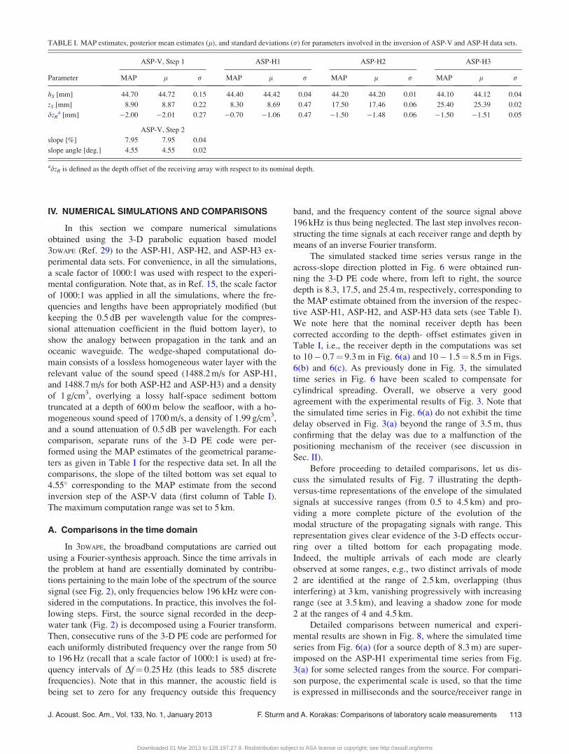
TABLE I. MAP estimates, posterior mean estimates (l), and standard deviations (r) for parameters involved in the inversion of ASP-V and ASP-H data sets.
ASP-V, Step 1 ASP-H1 ASP-H2 ASP-H3
Parameter MAP l r MAP l r MAP l r MAP l r
hS [mm] 44.70 44.72 0.15 44.40 44.42 0.04 44.20 44.20 0.01 44.10 44.12 0.04
zS [mm] 8.90 8.87 0.22 8.30 8.69 0.47 17.50 17.46 0.06 25.40 25.39 0.02
dzRa [mm] �2.00 �2.01 0.27 �0.70 �1.06 0.47 �1.50 �1.48 0.06 �1.50 �1.51 0.05
ASP-V, Step 2
slope [%] 7.95 7.95 0.04
slope angle [deg.] 4.55 4.55 0.02
adzR is defined as the depth offset of the receiving array with respect to its nominal depth.
J. Acoust. Soc. Am., Vol. 133, No. 1, January 2013 F. Sturm and A. Korakas: Comparisons of laboratory scale measurements 113
Downloaded 01 Mar 2013 to 128.197.27.9. Redistribution subject to ASA license or copyright; see http://asadl.org/terms

meters. In addition, the amplitude of both numerical and
experimental signals has been normalized to unity by divid-
ing, at each range, the time series by their maximum values.
Note finally that the experimental signals have been
low-pass filtered (with a cut-off frequency of 196 kHz) in
order to remove the higher-frequency content that was not
taken into account in the 3-D PE broadband computations.
For each receiver range, we observe a very good agreement,
FIG. 6. Results of 3-D numerical simulations with 3DWAPE with a scale factor of 1000:1. Stacked time series versus source/receiver range in the across-slope
direction for a source depth of (a) 8.3 m (all modes are excited), (b) 17.5 m (mode 3 is weakly excited), (c) 25.4 m (both modes 2 and 4 are weakly excited)
and at a receiver depth of (a) 9.3 m, (b) and (c) 8.5 m.
FIG. 7. Results of 3-D numerical simulations with 3DWAPE with a scale factor of 1000:1. Depth-versus-time representation at successive source/receiver ranges
(from 0.5 to 4.5 km) in the across-slope direction. The source depth is 8.3 m (all modes are excited) and the water depth is 44.4 m.
114 J. Acoust. Soc. Am., Vol. 133, No. 1, January 2013 F. Sturm and A. Korakas: Comparisons of laboratory scale measurements
Downloaded 01 Mar 2013 to 128.197.27.9. Redistribution subject to ASA license or copyright; see http://asadl.org/terms

both in phase and relative amplitude, between the experi-
mental and simulated results, demonstrating that the 3-D PE
broadband computations are able to reproduce the experi-
mentally recorded data with fine details.
B. Comparisons in the frequency domain
Predicted transmission loss (TL) versus across-slope
range obtained with the 3-D PE code are now compared to
experimental TL curves. The experimental TL curves are
extracted from the ASP-H data set, at any desired frequency
within the bandwidth of the source signal, by means of Fou-
rier transforms of the time series. Recall that during the
ASP-H1, ASP-H2, and ASP-H3 measurements, as described
in Sec. II, the time signals were recorded at a single receiver
depth (10 mm) and at several distances between 0.1 and 5 m
with a range increment of 0.005 m, thus providing a suffi-
ciently fine representation of the acoustic field in range.
Let us first compare the numerical results to the experi-
mental data at the frequency of 150 kHz, being close to the
dominant frequency of the source signal. The comparisons
are displayed in Fig. 9. The experimental TL curves are rep-
resented by the gray traces connecting the experimental data
points indicated by the data markers. From top to bottom,
the experimental TL curves were respectively extracted from
the ASP-H1, ASP-H2, and ASP-H3 data sets, recalling that
these correspond to nominal source depths of 10 mm (where
all modes are excited), 19 mm (where mode 3 is weakly
excited), and 26.9 mm (where both modes 2 and 4 are
weakly excited), in the respective order. The black curves in
Fig. 9 represent TL curves as predicted by the 3-D PE model
3DWAPE at a scale of 1000:1. Note, however, that the ex-
perimental scale is used (for time and range) on the figures
for the purpose of comparison. Let us first note that the inter-
ference patterns in each curve of Fig. 9 reveal the cut-off
ranges of each mode at the frequency of 150 Hz. Indeed, the
ranges of 1.3, 2, and 3 m can be identified as the approximate
cut-off ranges of modes 4, 3, and 2, respectively, where the
FIG. 8. Comparisons in the time domain. Time series in the across-slope direc-
tion at a fixed receiver depth and several ranges: (a) 2 m, (b) 2.5 m, (c) 3 m, and
(d) 3.5 m. For each subplot, the thick gray line corresponds to the experimen-
tally recorded ASP-H1 data (source depth: 10 mm; receiver depth: 10 mm) and
the thin black line corresponds to the numerical solution (source depth: 8.3 m;
receiver depth: 9.3 m) obtained running the 3-D PE based code 3DWAPE.
FIG. 9. Comparisons in the frequency domain. TL-versus-range curves (re-
ceiver depth: 10 mm, across-slope direction) at 150 kHz extracted from the
experimental data (gray lines with data marker) corresponding to a source
depth of (a) 10 mm (ASP-H1; all modes are excited), (b) 19 mm (ASP-H2;
mode 3 is weakly excited), (c) 26.9 mm (ASP-H3; both modes 2 and 4 are
weakly excited). The black solid lines represent the corresponding 3-D PE
solutions whose source and receiver depths are given in Table I.
J. Acoust. Soc. Am., Vol. 133, No. 1, January 2013 F. Sturm and A. Korakas: Comparisons of laboratory scale measurements 115
Downloaded 01 Mar 2013 to 128.197.27.9. Redistribution subject to ASA license or copyright; see http://asadl.org/terms

intensity abruptly decreases. The predicted TL curves in
Fig. 9 are in very good agreement with the experimental
ones. Nevertheless, a slight shift in phase can be observed at
some ranges, as, for instance, between the ranges of 2 and
FIG. 10. Comparison in the frequency domain. TL-versus-range curve (re-
ceiver depth: 10 mm, across-slope direction) extracted from the ASP-H1 ex-
perimental data (gray line with data marker) at 150 kHz. The black solid line
represents the corresponding 3-D PE solution whose source and receiver
depths are given in Table I. The sound speed in the sediment is 1740 m/s
(instead of 1700 m/s as in all other computations).
FIG. 11. Left panel: Transmission loss (in dB re 1 m) at 150 Hz (vertical sli-
ces in the across-slope direction) corresponding to 3-D PE computations with
a scale factor of 1000:1 considering an omnidirectional point source located
at a depth of (a) 8.3 m (all modes are excited), (b) 17.5 m (mode 3 is weakly
excited), and (c) 25.4 m (both modes 2 and 4 are weakly excited). On the right
panel are shown the shapes of the four propagating modes as a function of
depth. On each panel, the position of the source is indicated by a black circle.
FIG. 12. Comparisons in the frequency domain at several frequencies. TL-versus-range curves (receiver depth: 10 mm, across-slope direction) extracted from
the ASP-H1 experimental data (gray lines with data marker) at four frequencies: (a) 122 kHz, (b) 141.6 kHz, (c) 161.13 kHz, (d) 180.05 kHz. The source depth
is 10 mm (all modes are excited). The black solid lines represent the corresponding 3-D PE solutions whose source and receiver depths are given in Table I.
116 J. Acoust. Soc. Am., Vol. 133, No. 1, January 2013 F. Sturm and A. Korakas: Comparisons of laboratory scale measurements
Downloaded 01 Mar 2013 to 128.197.27.9. Redistribution subject to ASA license or copyright; see http://asadl.org/terms
3 m in Fig. 9(a), where the 3-D effects of mode 2 are more
pronounced. It is worth noting that running the 3-D PE code
with a different value for the sound speed in the sediment
can lead to an improvement at some ranges but deteriorates
the quality of the comparisons at others. For instance, the
comparisons obtained carrying out the simulations with a ho-
mogeneous bottom sound speed of 1740 m/s (instead of
1700 m/s) are shown in Fig. 10. Note that this specific value
of the bottom sound speed resulted in good comparisons
over a flat bottom in the past. As seen in Fig. 10, the compar-
isons with the experimental data for a titled bottom, though
better at some ranges (for instance, between 2 and 3 m) dete-
riorate significantly at longer ranges.
Overall, the 3-D PE model is able to accurately repro-
duce the acoustic field in the tank and correctly predict the
3-D propagation effects to which the modes are being sub-
jected. Furthermore, by construction, the 3D PE computa-
tions provide the complete picture in the waveguide (i.e., in
range, depth, and azimuth) without additional effort. For
instance, Fig. 11 represents TL versus across-slope range
and depth as computed by the 3DWAPE code for the respective
comparisons of Fig. 9. In this representation, the cut-off
ranges are recognized in a more straightforward manner.
Figure 12 shows comparisons of predicted and experi-
mental TL curves extracted from the ASP-H1 data set at four
additional frequencies: 122, 141.6, 161.13, and 180.05 kHz.
At each frequency, the predicted TL curves closely track the
detailed variations in the experimental TL curves, and this
could be expected, since a broadband likelihood function
was used when inverting the data. Note finally how the cut-
off of each mode is shifted out in range with increasing
frequency. This effect is known in the literature as the fre-
quency dependence of the mode cut-off range.
V. CONCLUDING REMARKS
In this paper, laboratory scale measurements of 3-D
acoustic propagation in a penetrable wedge were compared
with predictions by the 3-D parabolic equation code 3DWAPE.
A first comparison using the parameter values measured in
the tank, although encouraging, suggested a refinement was
required. A subspace inversion approach, to overcome the
significant CPU time requirements of 3-D computations, was
used to refine the geometrical parameters (source depth, re-
ceiver depth, and water depth) and the slope, within the mar-
gins of their experimental uncertainties. The inversion of the
data turned out to be a crucial step in successfully achieving
the comparisons. Using the refined parameter values, the
3-D PE model was able to accurately reproduce the fine
details of the measured 3-D acoustic field in the tank, both in
the time and in the frequency domain, demonstrating the full
potential of the model at hand. In addition, it is worth noting
that, by construction, the 3-D PE model provides the entire
acoustic field in the waveguide (in range, depth, and azi-
muth) with no additional effort.
Let us note that the strong assumption of a homogeneous
bottom half-space adopted in the 3-D PE computations,
though subject to discussion, turned out to be reasonable in the
actual context. Among others, this assumption involves
neglecting the potential presence of shear waves propagating
in the bottom when inverting the data. Note that the same
assumption led to satisfactory agreement between theory and
experiment during the calibration phase over a flat bottom,
even though satisfactory comparisons were also achieved
using a very low shear wave speed value. In its present form,
the 3-D PE model 3DWAPE handles multilayered fluid bottoms
alone, but can be modified to incorporate the effect of a low
shear wave speed in the bottom using an equivalent fluid
approximation based on the complex density approach pro-
posed by Zhang and Tindle.30 This modification, being quite
straightforward and having already been successfully applied
in a 3-D PE code,31 will permit one to perform additional com-
parisons considering a shear-supporting bottom. This is cur-
rently underway. As a final note, the data collected during this
experimental campaign have an overall promising potential to
provide a real-data benchmark for 3-D model validation and
performance comparison.
APPENDIX: OBJECTIVE FUNCTIONS
Let the N-length complex vector dl denote the observed
data at frequency fl on an N-element receiving array at some
location in the water column, and wl(m) the replica vector
provided by an ocean acoustic propagation model as a func-
tion of the M-length parameters vector m to be recovered.
Assuming additive errors, the observed data and replica vec-
tors are related through
dl ¼ SlwlðmÞ þ nl; (A1)
where Sl denotes the complex source strength at frequency fland nl the error vector including both experimental and
theory errors. When the error term is assumed zero-mean
complex Gaussian distributed with diagonal covariance ma-
trix �lI, i.e., spatially uncorrelated, the broadband likelihood
function is written
Lðm; S; vÞ ¼YL
l¼1
ðpvlÞ�Nexp �kdl � SlwlðmÞk2
vl
" #;
(A2)
where it is further assumed that the errors are uncorrelated
across frequency. When the source spectrum and the var-
iance are unknown, they are replaced by their estimates
obtained by maximizing Eq. (A2).
The first expression used herein is derived for complex
acoustic pressure fields, i.e., using both magnitude and
phase, following
L1ðmÞ ¼YL
l¼1
ðpv̂lÞ�Nexp �
/l;1ðmÞv̂l
� �; (A3)
where /l,1 is an objective function related to the Bartlett
power given as23–25
/l;1ðmÞ ¼ kdlk2 � jw�l ðmÞdlj2
kwlðmÞk2; (A4)
J. Acoust. Soc. Am., Vol. 133, No. 1, January 2013 F. Sturm and A. Korakas: Comparisons of laboratory scale measurements 117
Downloaded 01 Mar 2013 to 128.197.27.9. Redistribution subject to ASA license or copyright; see http://asadl.org/terms

and v̂l is a global maximum likelihood estimate of the var-
iance obtained as
v̂l ¼1
N/l;1ðm̂Þ (A5)
and evaluated at the maximum likelihood solution m̂. This
latter is obtained by minimizing25
UðmÞ ¼YL
l¼1
/l;1ðmÞ: (A6)
over all m. Note here that N in Eq. (A5) should be replaced
by the effective number of uncorrelated receivers along the
array which is usually equivalent to the number of trapped
modes contributing at the array.32 The expression (A3) leads
to the matched-field inversion technique where Eq. (A4) is
recognized as the normalized Bartlett power.
The second expression of the broadband likelihood
function used herein is derived using the magnitude of the
data alone:
L2ðmÞ ¼YL
t¼1
/l;2ðmÞ�N=2YNn¼1
jwl;nðmÞj�1=2; (A7)
where wl,n(m) is the nth component of vector wl(m) and the
objective function is given as
/l;2ðmÞ ¼ kdlk2 � jwlðmÞj�jdljkwlðmÞk
� �2
: (A8)
Using Eq. (A7) is equivalent to fitting experimental and pre-
dicted transmission loss curves along the array.
1A. Tolstoy, “3-D propagation issues and models,” J. Comput. Acoust. 4,
243–271 (1996).2K. D. Heaney and J. J. Murray, “Measurements of three-dimensional prop-
agation in a continental shelf environment,” J. Acoust. Soc. Am. 125,
1394–1402 (2009).3M. S. Ballard, Y.-T. Lin, and J. F. Lynch,“Horizontal refraction of propa-
gating sound due to seafloor scours over a range-dependent layered bottom
on the New Jersey shelf,” J. Acoust. Soc. Am. 131, 2587–2598 (2012).4L. Y. S. Chiu, A. Y. Y. Chang, C.-F. Chen, R.-C. Wei, Y.-J. Yang, and D.
B. Reeder,“Three dimensional acoustic simulation of an acoustic refrac-
tion by a nonlinear internal wave in a wedge bathymetry,” J. Comput.
Acoust. 18, 279–296 (2010).5D. B. Reeder, L. Y. S. Chiu, and C.-F. Chen, “Experimental evidence of
horizontal refraction by nonlinear internal waves of elevation in shallow
water in the South China Sea: 3D versus Nx2D acoustic propagation mod-
eling,” J. Comput. Acoust. 18, 267–278 (2010).6M. S. Ballard, “Modeling three-dimensional propagation in a continental
shelf environment,” J. Acoust. Soc. Am. 131, 1969–1977 (2012).7L. Hsieh, Y. Lin, and C. Chen, “Three dimensional wide angle azimuthal
PE solution to modified benchmark problems,” J. Acoust. Soc. Am. 115,
2579 (2004).8L. Hsieh, C. Chen, M. Yuan, and Y. Lin, “Azimuthal limitation in 3D PE
approximation for underwater acoustic propagation,” J. Comput. Acoust.
15, 221–233 (2007).9L. Y. S. Chiu, Y.-T. Lin, C.-F. Chen, T. F. Duda, and B. Calder, “Focused
sound from three-dimensional sound propagation effects over a submarine
canyon,” J. Acoust. Soc. Am. 129, EL260–EL266 (2011).
10M. E. Austin and N. R. Chapman, “The use of tessellation in three-
dimensional parabolic equation modeling,” J. Comput. Acoust. 19, 221–
239 (2011).11P. Borejko, “An analysis of cross-slope pulse propagation in a shallow
water wedge,” in Proceedings of the 10th Conference on UnderwaterAcoustics, edited by T. Akal, Istanbul, Turkey (2010).
12Y.-T. Lin and T. F. Duda, “A higher-order split-step fourier parabolic-
equation sound propagation solution scheme,” J. Acoust. Soc. Am. 132,
EL61–EL67 (2012).13Y.-T. Lin and J. F. Lynch, “Analytical study of the horizontal ducting
of sound by an oceanic front over a slope,” J. Acoust. Soc. Am. 131,
EL1–EL7 (2011).14F. Sturm, “Investigation of 3-D benchmark problems in underwater acous-
tics: A uniform approach,” in Proceedings of the 9th European Confer-ence on Underwater Acoustics, edited by M. E. Zakharia, D. Cassereau,
and F. Lupp�e, Paris, France (2008), Vol. 2, pp. 759–764.15J. M. Collis, W. L. Siegmann, M. D. Collins, H. J. Simpson, and R. J.
Soukup, “Comparison of simulations and data from a seismo-acoustic tank
experiment,” J. Acoust. Soc. Am. 122, 1987–1993 (2007).16J. D. Schneiderwind, J. M. Collis, and H. J. Simpson, “Elastic pekeris
waveguide normal mode solution comparisons against laboratory data,”
J. Acoust. Soc. Am. 132, EL182–EL188 (2012).17C. H. Harrison, “Acoustic shadow zones in the horizontal plane,”
J. Acoust. Soc. Am. 65, 56–61 (1979).18M. J. Buckingham, “Theory of three-dimensional acoustic propagation in
a wedgelike ocean with a penetrable bottom,” J. Acoust. Soc. Am. 82,
198–210 (1987).19F. Sturm, J.-P. Sessarego, and D. Ferrand, “Laboratory scale measure-
ments of across-slope sound propagation over a wedge-shaped bottom,” in
2nd International Conference & Exhibition on Underwater AcousticMeasurements: Technologies & Results, edited by J. S. Papadakis and
L. Bj€orno, Heraklion, Crete, Greece (2007), Vol. 3, pp. 1151–1156.20P. Papadakis, M. Taroudakis, F. Sturm, P. Sanchez, and J.-P. Sessare-
go,“Scaled laboratory experiments of shallow water acoustic propagation:
Calibration phase,” Acta Acust. Acust. 94, 676–684 (2008).21N. Bilaniuk and G. S. K. Wong, “Speed of sound in pure water as a func-
tion of temperature,” J. Acoust. Soc. Am. 93, 1609–1612 (1993).22A. Korakas, F. Sturm, J.-P. Sessarego, and D. Ferrand, “Scaled model
experiment of long-range across-slope pulse propagation in a penetrable
wedge,” J. Acoust. Soc. Am. 126, EL22–EL27 (2009).23P. Gerstoft and C. F. Mecklenbrauker, “Ocean acoustic inversion with esti-
mation of a posteriori probability distributions,” J. Acoust. Soc. Am. 104,
808–819 (1998).24S. E. Dosso and G. Birdsall, “Quantifying uncertainties in geoacoustic
inversion I: A fast Gibbs sampler approach,” J. Acoust. Soc. Am. 111,
129–142 (2002).25C. F. Mecklenbrauker and P. Gerstoft, “Objective functions for ocean
acoustic inversion derived by likelihood methods,” J. Comput. Acoust. 8,
259–270 (2000).26M. K. Sen and P. L. Stoffa, “Bayesian inference, Gibbs’ sampler and
uncertainty estimation in geophysical inversion,” Geophys. Prospect. 44,
313–350 (1996).27J. A. Fawcett, “Modeling three-dimensional propagation in an oceanic
wedge using parabolic equation methods,” J. Acoust. Soc. Am. 93, 2627–
2632 (1993).28A. Korakas and F. Sturm, “On the feasibility of a matched-field inversion
in a three- dimensional environment ignoring out-of-plane propagation,”
IEEE J. Oceanic Eng. 36, 716–727 (2011).29F. Sturm, “Numerical study of broadband sound pulse propagation in
three-dimensional oceanic waveguides,” J. Acoust. Soc. Am. 117, 1058–
1079 (2005).30Z. Y. Zhang and C. T. Tindle, “Improved equivalent fluid approximations
for a low shear speed ocean bottom,” J. Acoust. Soc. Am. 98, 3391–3396
(1995).31G. H. Brooke, D. J. Thomson, and G. R. Ebbeson, “PECan: A Canadian
parabolic equation model for underwater sound propagation,” J. Comput.
Acoust. 9, 69–100 (2001).32S. E. Dosso and G. Birdsall, “Quantifying uncertainties in geoacoustic
inversion II. Ap- plication to broadband, shallow-water data,” J. Acoust.
Soc. Am. 111, 143–159 (2002).
118 J. Acoust. Soc. Am., Vol. 133, No. 1, January 2013 F. Sturm and A. Korakas: Comparisons of laboratory scale measurements
Downloaded 01 Mar 2013 to 128.197.27.9. Redistribution subject to ASA license or copyright; see http://asadl.org/terms


![Page 1© Crown copyright 2004 Introduction to upper air measurements with radiosondes and other in situ observing systems [2] Factors affecting comparisons](https://cdn.vdocuments.us/doc/165x107/551a3290550346545e8b4aad/page-1-crown-copyright-2004-introduction-to-upper-air-measurements-with-radiosondes-and-other-in-situ-observing-systems-2-factors-affecting-comparisons.jpg)


