BackgroundML model fitting comparison
GMM model fitting comparisonImpacts
Comparing estimation methods for spatialeconometrics
Recent Advances in Spatial Econometrics (in honor of JamesLeSage), ERSA 2012
Roger Bivand Gianfranco Piras
NHH Norwegian School of Economics
Regional Research Institute at West Virginia University
Thursday, 23 August 2012
Roger Bivand, Gianfranco Piras Comparing estimation methods

BackgroundML model fitting comparison
GMM model fitting comparisonImpacts
Outline
Recent advances in spatial econometrics model fittingtechniques have made it more desirable to be able to compareresults
Results should correspond between implementations usingdifferent applications
A broad range of model fitting techniques are provided by thecontributed R packages for spatial econometrics
These model fitting techniques are associated with methodsfor estimating impacts and some tests, which will also bepresented and compared
Roger Bivand, Gianfranco Piras Comparing estimation methods
BackgroundML model fitting comparison
GMM model fitting comparisonImpacts
Background
The use of spatial econometrics tools was widened by the easewith which methods and examples presented in Anselin (1988)could be reproduced using SpaceStatTM, written in GaussTM
It was rapidly complemented by the Spatial Econometricstoolbox for MatlabTM, provided as source code together withextensive documentation
A suite of commands for spatial data analysis for use withStataTM was provided by Maurizio Pisati, and macros forMinitabTM and SASTM were also made available
The thrust of SpaceStatTM has largely been taken over byGeoDa (Anselin et al. 2006), and more recently byOpenGeoDa
Roger Bivand, Gianfranco Piras Comparing estimation methods

BackgroundML model fitting comparison
GMM model fitting comparisonImpacts
Today’s software
There is now much more software available for spatialeconometrics
StataTM with sppack and MatlabTM with SpatialEconometrics Toolbox are mainstream programmes; theMatlabTM toolbox remains in the public domain, and has acommunity of contributors
OpenGeoDa and PySAL are open source, with code hosted onGoogle, binary versions for common platforms, and acommunity of users
R with spdep, sphet, McSpatial and other contributedpackages is open source, and the packages are cross-platform;the packages also have a community of users and developers
Roger Bivand, Gianfranco Piras Comparing estimation methods
BackgroundML model fitting comparison
GMM model fitting comparisonImpacts
Why compare?
In the spirit of Rey (2009), this comparison will attempt toexamine some features of the implementation of functions forfitting spatial econometrics models
Firstly, it may be useful to show which kinds of functions forcreating spatial weights, for diagnostics, and for model fittingare available
Next, it is comforting when one can show that fitting thesame model on the same data using different implementationsgives the same results
Finally, if the results are not the same, it is helpful to be ableto show why they vary, possibly because of different designchoices in implementation
Roger Bivand, Gianfranco Piras Comparing estimation methods

BackgroundML model fitting comparison
GMM model fitting comparisonImpacts
Data set: Ward and Gleditsch 2008
The data set used for comparison here is taken from a Sagevolume Spatial Regression Models by Ward and Gleditsch(2008), with political science data for 158 countries
The model they explore is the relationship between democracyscores (POLITY IV indicators) and the logarithm of countryGDP per capita in 2002
They treat countries as neighbours with non-zero spatialweights if their borders are closer than 200km from each other;data and weights are available for download from their site
They were among the first to examine the effects of feedbackin spatial regression models
Roger Bivand, Gianfranco Piras Comparing estimation methods

BackgroundML model fitting comparison
GMM model fitting comparisonImpacts
Spatial weights
Creating spatial weights is a necessary step in using areal data,perhaps just to check that there is no remaining spatial patterningin residuals
The Matlab SE toolbox provides functions for creating nearestneighbour and triangulation contiguity weights, and for reading GALfiles
A number of functions are included in the R spdep package tocreate neighbours, and from them weights; GAL and GWT files maybe read and written
Weights may be constructed using functions in GeoDa, and in Pysalusing Python programming; GAL and GWT files may be read andwritten
The Stata spmat command provides for the creation of a number ofdifferent kinds of weights, and for file import and export
Roger Bivand, Gianfranco Piras Comparing estimation methods
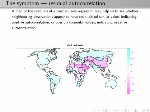
The symptom — residual autocorrelationA map of the residuals of a least squares regression may help us to see whether
neighbouring observations appear to have residuals od similar value, indicating
positive autocorrelation, or possibly dissimilar values, indicating negative
autocorrelation:
OLS residuals
−15
−10
−5
0
5
10
15

BackgroundML model fitting comparison
GMM model fitting comparisonImpacts
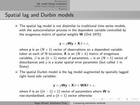
Spatial lag and Durbin models
The spatial lag model is not dissimilar to traditional time series models,with the autocorrelation process in the dependent variable controlled bythe exogenous matrix of spatial weights W (Ord 1975):
y = ρWy + Xβ + ε,
where y is an (N × 1) vector of observations on a dependent variabletaken at each of N locations, X is an (N × k) matrix of exogenousvariables, β is an (k × 1) vector of parameters, ε is an (N × 1) vector ofdisturbances and ρ is a scalar spatial error parameter (but called λ inStata)
The spatial Durbin model is the lag model augmented by spatially laggedright hand side variables:
y = ρWy + Xβ + WXθ + ε,
where θ is an ((k − 1)× 1) vector of parameters where W isrow-standardised, and a (k × 1) vector otherwise
Roger Bivand, Gianfranco Piras Comparing estimation methods
BackgroundML model fitting comparison
GMM model fitting comparisonImpacts
Spatial lag and Durbin models
The spatial lag model is not dissimilar to traditional time series models,with the autocorrelation process in the dependent variable controlled bythe exogenous matrix of spatial weights W (Ord 1975):
y = ρWy + Xβ + ε,
where y is an (N × 1) vector of observations on a dependent variabletaken at each of N locations, X is an (N × k) matrix of exogenousvariables, β is an (k × 1) vector of parameters, ε is an (N × 1) vector ofdisturbances and ρ is a scalar spatial error parameter (but called λ inStata)
The spatial Durbin model is the lag model augmented by spatially laggedright hand side variables:
y = ρWy + Xβ + WXθ + ε,
where θ is an ((k − 1)× 1) vector of parameters where W isrow-standardised, and a (k × 1) vector otherwise
Roger Bivand, Gianfranco Piras Comparing estimation methods

BackgroundML model fitting comparison
GMM model fitting comparisonImpacts
Spatial lag model log-likelihood function
`(β, ρ, σ2) = −N
2ln 2π − N
2lnσ2 + ln |I− ρW|
− 1
2σ2
[y′(I− ρW)′(I− X(X′X)−1X′)(I− ρW)y
]and β = (X′X)−1(I− ρW)y, where ρ is the ML estimate.Unlike the time series case, the logarithm of the determinant of the(N × N) asymmetric matrix (I− ρW) does not tend to zero withincreasing sample size; it constrains the parameter values to theirfeasible range between the inverses of the smallest and largesteigenvalues of W, since for positive autocorrelation, as ρ → 1,ln |I− ρW| → −∞
Roger Bivand, Gianfranco Piras Comparing estimation methods
BackgroundML model fitting comparison
GMM model fitting comparisonImpacts
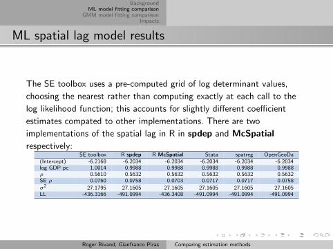
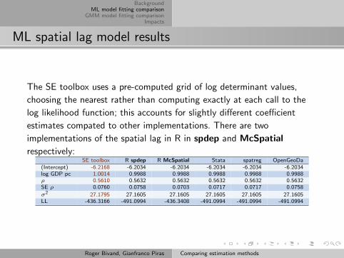
ML spatial lag model results
The SE toolbox uses a pre-computed grid of log determinant values,
choosing the nearest rather than computing exactly at each call to the
log likelihood function; this accounts for slightly different coefficient
estimates compated to other implementations. There are two
implementations of the spatial lag in R in spdep and McSpatial
respectively:SE toolbox R spdep R McSpatial Stata spatreg OpenGeoDa
(Intercept) -6.2168 -6.2034 -6.2034 -6.2034 -6.2034 -6.2034log GDP pc 1.0014 0.9988 0.9988 0.9988 0.9988 0.9988ρ 0.5610 0.5632 0.5632 0.5632 0.5632 0.5632SE ρ 0.0760 0.0758 0.0703 0.0717 0.0717 0.0758
σ2 27.1795 27.1605 27.1605 27.1605 27.1605 27.1605LL -436.3166 -491.0994 -436.3408 -491.0994 -491.0994 -491.0994
Roger Bivand, Gianfranco Piras Comparing estimation methods
BackgroundML model fitting comparison
GMM model fitting comparisonImpacts
ML spatial lag model results
The SE toolbox uses a pre-computed grid of log determinant values,
choosing the nearest rather than computing exactly at each call to the
log likelihood function; this accounts for slightly different coefficient
estimates compated to other implementations. There are two
implementations of the spatial lag in R in spdep and McSpatial
respectively:SE toolbox R spdep R McSpatial Stata spatreg OpenGeoDa
(Intercept) -6.2168 -6.2034 -6.2034 -6.2034 -6.2034 -6.2034log GDP pc 1.0014 0.9988 0.9988 0.9988 0.9988 0.9988ρ 0.5610 0.5632 0.5632 0.5632 0.5632 0.5632SE ρ 0.0760 0.0758 0.0703 0.0717 0.0717 0.0758
σ2 27.1795 27.1605 27.1605 27.1605 27.1605 27.1605LL -436.3166 -491.0994 -436.3408 -491.0994 -491.0994 -491.0994
Roger Bivand, Gianfranco Piras Comparing estimation methods

BackgroundML model fitting comparison
GMM model fitting comparisonImpacts
ML spatial lag model differences I
There are two major discrepancies in the table of results: the first is that
the log-likelihood values at the optimimum differ between R McSpatial
and the SE toolbox and the rest.
SE toolbox R spdep R McSpatial Stata spatreg OpenGeoDa(Intercept) -6.2168 -6.2034 -6.2034 -6.2034 -6.2034 -6.2034log GDP pc 1.0014 0.9988 0.9988 0.9988 0.9988 0.9988ρ 0.5610 0.5632 0.5632 0.5632 0.5632 0.5632SE ρ 0.0760 0.0758 0.0703 0.0717 0.0717 0.0758
σ2 27.1795 27.1605 27.1605 27.1605 27.1605 27.1605LL -436.3166 -491.0994 -436.3408 -491.0994 -491.0994 -491.0994
The reason appears to be that π in the log likelihood calculation is not
multiplied by 2 in these cases, but is in the remainder. If we convert the
R McSpatial value of −436.3408 by subtracting n2 log(π) (line 65 in file
McSpatial/R/sarml.R), and adding n2 log(2π), we get −491.0752.
Similarly, correcting the SE toolbox value of −436.3166, we get
−491.0752 (line 453 file spatial/sar models/sar.m). The same kind of
difference appears in other reported SE toolbox log likelihood valuesRoger Bivand, Gianfranco Piras Comparing estimation methods

BackgroundML model fitting comparison
GMM model fitting comparisonImpacts
ML spatial lag model differences II
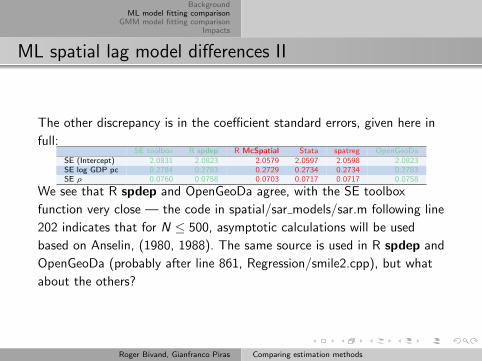
The other discrepancy is in the coefficient standard errors, given here in
full:SE toolbox R spdep R McSpatial Stata spatreg OpenGeoDa
SE (Intercept) 2.0831 2.0823 2.0579 2.0597 2.0598 2.0823SE log GDP pc 0.2784 0.2783 0.2729 0.2734 0.2734 0.2783SE ρ 0.0760 0.0758 0.0703 0.0717 0.0717 0.0758
We see that R spdep and OpenGeoDa agree, with the SE toolbox
function very close — the code in spatial/sar models/sar.m following line
202 indicates that for N ≤ 500, asymptotic calculations will be used
based on Anselin, (1980, 1988). The same source is used in R spdep and
OpenGeoDa (probably after line 861, Regression/smile2.cpp), but what
about the others?
Roger Bivand, Gianfranco Piras Comparing estimation methods
BackgroundML model fitting comparison
GMM model fitting comparisonImpacts
ML spatial lag model differences II
The other discrepancy is in the coefficient standard errors, given here in
full:SE toolbox R spdep R McSpatial Stata spatreg OpenGeoDa
SE (Intercept) 2.0831 2.0823 2.0579 2.0597 2.0598 2.0823SE log GDP pc 0.2784 0.2783 0.2729 0.2734 0.2734 0.2783SE ρ 0.0760 0.0758 0.0703 0.0717 0.0717 0.0758
We see that R spdep and OpenGeoDa agree, with the SE toolbox
function very close — the code in spatial/sar models/sar.m following line
202 indicates that for N ≤ 500, asymptotic calculations will be used
based on Anselin, (1980, 1988). The same source is used in R spdep and
OpenGeoDa (probably after line 861, Regression/smile2.cpp), but what
about the others?
Roger Bivand, Gianfranco Piras Comparing estimation methods

BackgroundML model fitting comparison
GMM model fitting comparisonImpacts
ML spatial lag model differences II — more
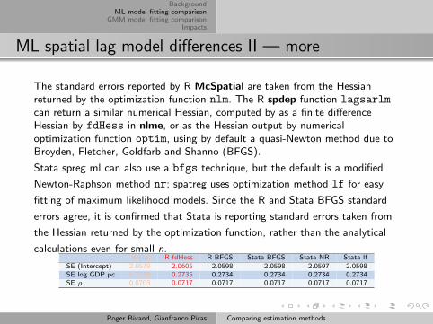
The standard errors reported by R McSpatial are taken from the Hessianreturned by the optimization function nlm. The R spdep function lagsarlmcan return a similar numerical Hessian, computed by as a finite differenceHessian by fdHess in nlme, or as the Hessian output by numericaloptimization function optim, using by default a quasi-Newton method due toBroyden, Fletcher, Goldfarb and Shanno (BFGS).
Stata spreg ml can also use a bfgs technique, but the default is a modified
Newton-Raphson method nr; spatreg uses optimization method lf for easy
fitting of maximum likelihood models. Since the R and Stata BFGS standard
errors agree, it is confirmed that Stata is reporting standard errors taken from
the Hessian returned by the optimization function, rather than the analytical
calculations even for small n.R nlm R fdHess R BFGS Stata BFGS Stata NR Stata lf
SE (Intercept) 2.0579 2.0605 2.0598 2.0598 2.0597 2.0598SE log GDP pc 0.2729 0.2735 0.2734 0.2734 0.2734 0.2734SE ρ 0.0703 0.0717 0.0717 0.0717 0.0717 0.0717
Roger Bivand, Gianfranco Piras Comparing estimation methods
BackgroundML model fitting comparison
GMM model fitting comparisonImpacts
ML spatial lag model differences II — more
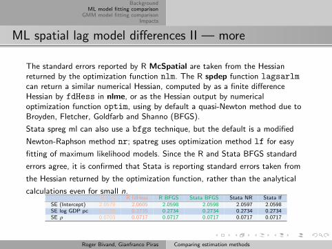
The standard errors reported by R McSpatial are taken from the Hessianreturned by the optimization function nlm. The R spdep function lagsarlmcan return a similar numerical Hessian, computed by as a finite differenceHessian by fdHess in nlme, or as the Hessian output by numericaloptimization function optim, using by default a quasi-Newton method due toBroyden, Fletcher, Goldfarb and Shanno (BFGS).
Stata spreg ml can also use a bfgs technique, but the default is a modified
Newton-Raphson method nr; spatreg uses optimization method lf for easy
fitting of maximum likelihood models. Since the R and Stata BFGS standard
errors agree, it is confirmed that Stata is reporting standard errors taken from
the Hessian returned by the optimization function, rather than the analytical
calculations even for small n.R nlm R fdHess R BFGS Stata BFGS Stata NR Stata lf
SE (Intercept) 2.0579 2.0605 2.0598 2.0598 2.0597 2.0598SE log GDP pc 0.2729 0.2735 0.2734 0.2734 0.2734 0.2734SE ρ 0.0703 0.0717 0.0717 0.0717 0.0717 0.0717
Roger Bivand, Gianfranco Piras Comparing estimation methods
BackgroundML model fitting comparison
GMM model fitting comparisonImpacts
ML spatial lag model differences II — more
The standard errors reported by R McSpatial are taken from the Hessianreturned by the optimization function nlm. The R spdep function lagsarlmcan return a similar numerical Hessian, computed by as a finite differenceHessian by fdHess in nlme, or as the Hessian output by numericaloptimization function optim, using by default a quasi-Newton method due toBroyden, Fletcher, Goldfarb and Shanno (BFGS).
Stata spreg ml can also use a bfgs technique, but the default is a modified
Newton-Raphson method nr; spatreg uses optimization method lf for easy
fitting of maximum likelihood models. Since the R and Stata BFGS standard
errors agree, it is confirmed that Stata is reporting standard errors taken from
the Hessian returned by the optimization function, rather than the analytical
calculations even for small n.R nlm R fdHess R BFGS Stata BFGS Stata NR Stata lf
SE (Intercept) 2.0579 2.0605 2.0598 2.0598 2.0597 2.0598SE log GDP pc 0.2729 0.2735 0.2734 0.2734 0.2734 0.2734SE ρ 0.0703 0.0717 0.0717 0.0717 0.0717 0.0717
Roger Bivand, Gianfranco Piras Comparing estimation methods
BackgroundML model fitting comparison
GMM model fitting comparisonImpacts
Maximum likelihood fitting differences
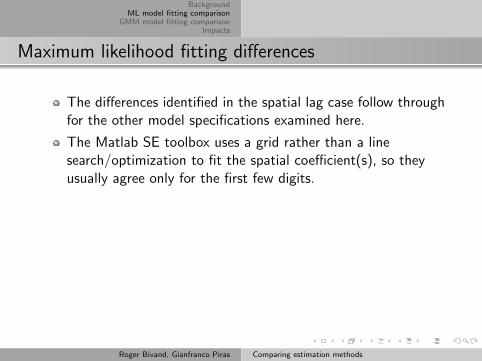
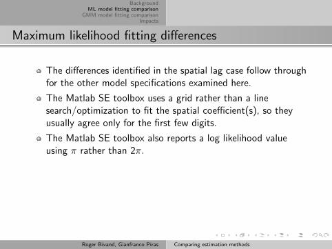
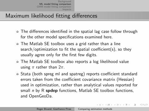
The differences identified in the spatial lag case follow throughfor the other model specifications examined here.
The Matlab SE toolbox uses a grid rather than a linesearch/optimization to fit the spatial coefficient(s), so theyusually agree only for the first few digits.
The Matlab SE toolbox also reports a log likelihood valueusing π rather than 2π.
Stata (both spreg ml and spatreg) reports coefficient standarderrors taken from the coefficient covariance matrix (Hessian)used in optimization, rather than analytical values reported forsmall n by R spdep functions, Matlab SE toolbox functions,and OpenGeoDa.
Roger Bivand, Gianfranco Piras Comparing estimation methods
BackgroundML model fitting comparison
GMM model fitting comparisonImpacts
Maximum likelihood fitting differences
The differences identified in the spatial lag case follow throughfor the other model specifications examined here.
The Matlab SE toolbox uses a grid rather than a linesearch/optimization to fit the spatial coefficient(s), so theyusually agree only for the first few digits.
The Matlab SE toolbox also reports a log likelihood valueusing π rather than 2π.
Stata (both spreg ml and spatreg) reports coefficient standarderrors taken from the coefficient covariance matrix (Hessian)used in optimization, rather than analytical values reported forsmall n by R spdep functions, Matlab SE toolbox functions,and OpenGeoDa.
Roger Bivand, Gianfranco Piras Comparing estimation methods
BackgroundML model fitting comparison
GMM model fitting comparisonImpacts
ML spatial Durbin model results
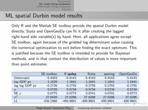
Only R and the Matlab SE toolbox provide the spatial Durbin model
directly, Stata and OpenGeoDa can fit it after creating the lagged
right-hand side variable(s) by hand. Here, all applications agree except
SE toolbox, again because of the gridded log determinant value causing
the numerical optimization to exit before finding the exact optimum. This
is justified because the SE toolbox is intended to provide for Bayesian
methods, and in that context the distribution of values is more important
than point estimates:
SE toolbox R spdep Stata spatreg OpenGeoDa(Intercept) -5.4303 -5.4143 -5.4143 -5.4143 -5.4143log GDP pc 1.1639 1.1641 1.1641 1.1641 1.1641lag log GDP pc -0.2726 -0.2755 -0.2755 -0.2755 -0.2755ρ 0.5720 0.5734 0.5734 0.5734 0.5734SE ρ 0.0775 0.0773 0.0741 0.0741 0.0773σ2 27.0420 27.0296 27.0296 27.0296 27.0296LL -436.1960 -490.9801 -490.9801 -490.9801 -490.9801
Roger Bivand, Gianfranco Piras Comparing estimation methods
BackgroundML model fitting comparison
GMM model fitting comparisonImpacts
Spatial error model
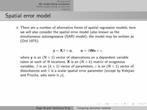
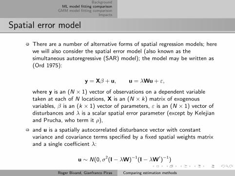
There are a number of alternative forms of spatial regression models; herewe will also consider the spatial error model (also known as thesimultaneous autoregressive (SAR) model); the model may be written as(Ord 1975):
y = Xβ + u, u = λWu + ε,
where y is an (N × 1) vector of observations on a dependent variabletaken at each of N locations, X is an (N × k) matrix of exogenousvariables, β is an (k × 1) vector of parameters, ε is an (N × 1) vector ofdisturbances and λ is a scalar spatial error parameter (except by Kelejianand Prucha, who term it ρ),
and u is a spatially autocorrelated disturbance vector with constantvariance and covariance terms specified by a fixed spatial weights matrixand a single coefficient λ:
u ∼ N(0, σ2(I− λW)−1(I− λW′)−1)
Roger Bivand, Gianfranco Piras Comparing estimation methods
BackgroundML model fitting comparison
GMM model fitting comparisonImpacts
Spatial error model
There are a number of alternative forms of spatial regression models; herewe will also consider the spatial error model (also known as thesimultaneous autoregressive (SAR) model); the model may be written as(Ord 1975):
y = Xβ + u, u = λWu + ε,
where y is an (N × 1) vector of observations on a dependent variabletaken at each of N locations, X is an (N × k) matrix of exogenousvariables, β is an (k × 1) vector of parameters, ε is an (N × 1) vector ofdisturbances and λ is a scalar spatial error parameter (except by Kelejianand Prucha, who term it ρ),
and u is a spatially autocorrelated disturbance vector with constantvariance and covariance terms specified by a fixed spatial weights matrixand a single coefficient λ:
u ∼ N(0, σ2(I− λW)−1(I− λW′)−1)
Roger Bivand, Gianfranco Piras Comparing estimation methods
BackgroundML model fitting comparison
GMM model fitting comparisonImpacts
Spatial error model log-likelihood function
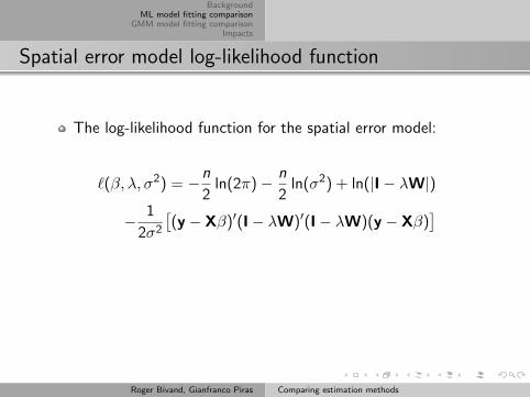
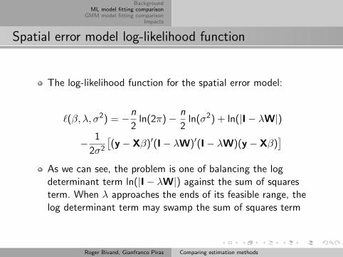
The log-likelihood function for the spatial error model:
`(β, λ, σ2) = −n
2ln(2π)− n
2ln(σ2) + ln(|I− λW|)
− 1
2σ2
[(y − Xβ)′(I− λW)′(I− λW)(y − Xβ)
]
As we can see, the problem is one of balancing the logdeterminant term ln(|I− λW|) against the sum of squaresterm. When λ approaches the ends of its feasible range, thelog determinant term may swamp the sum of squares term
Roger Bivand, Gianfranco Piras Comparing estimation methods
BackgroundML model fitting comparison
GMM model fitting comparisonImpacts
Spatial error model log-likelihood function
The log-likelihood function for the spatial error model:
`(β, λ, σ2) = −n
2ln(2π)− n
2ln(σ2) + ln(|I− λW|)
− 1
2σ2
[(y − Xβ)′(I− λW)′(I− λW)(y − Xβ)
]As we can see, the problem is one of balancing the logdeterminant term ln(|I− λW|) against the sum of squaresterm. When λ approaches the ends of its feasible range, thelog determinant term may swamp the sum of squares term
Roger Bivand, Gianfranco Piras Comparing estimation methods
BackgroundML model fitting comparison
GMM model fitting comparisonImpacts
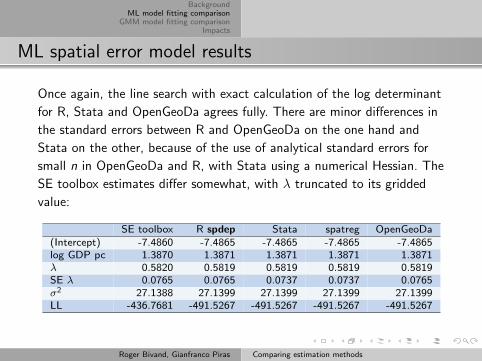
ML spatial error model results
Once again, the line search with exact calculation of the log determinant
for R, Stata and OpenGeoDa agrees fully. There are minor differences in
the standard errors between R and OpenGeoDa on the one hand and
Stata on the other, because of the use of analytical standard errors for
small n in OpenGeoDa and R, with Stata using a numerical Hessian. The
SE toolbox estimates differ somewhat, with λ truncated to its gridded
value:
SE toolbox R spdep Stata spatreg OpenGeoDa(Intercept) -7.4860 -7.4865 -7.4865 -7.4865 -7.4865log GDP pc 1.3870 1.3871 1.3871 1.3871 1.3871λ 0.5820 0.5819 0.5819 0.5819 0.5819SE λ 0.0765 0.0765 0.0737 0.0737 0.0765σ2 27.1388 27.1399 27.1399 27.1399 27.1399LL -436.7681 -491.5267 -491.5267 -491.5267 -491.5267
Roger Bivand, Gianfranco Piras Comparing estimation methods

BackgroundML model fitting comparison
GMM model fitting comparisonImpacts
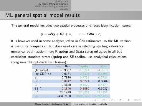
ML general spatial model results
The general model includes two spatial processes and faces identification issues:
y = ρWy + Xβ + u, u = λWu + ε,
It is however used in some analyses, often in GM estimators, so the ML version
is useful for comparison, but does need care in selecting starting values for
numerical optimization; here R spdep and Stata spreg ml agree in all but
coefficient standard errors (spdep and SE toolbox use analytical calculations,
spreg uses the optimization Hessian):SE toolbox R spdep Stata
(Intercept) -3.9367 -4.0211 -4.0210log GDP pc 0.6161 0.6301 0.6301ρ 0.7810 0.7735 0.7735SE ρ 0.0742 0.0771 0.0804λ -0.4650 -0.4479 -0.4479SE λ 0.1846 0.1880 0.1937σ2 23.1479 23.3251 23.3251LL -434.7130 -489.5175 -489.5175
Roger Bivand, Gianfranco Piras Comparing estimation methods
BackgroundML model fitting comparison
GMM model fitting comparisonImpacts
ML general spatial model results
The general model includes two spatial processes and faces identification issues:
y = ρWy + Xβ + u, u = λWu + ε,
It is however used in some analyses, often in GM estimators, so the ML version
is useful for comparison, but does need care in selecting starting values for
numerical optimization; here R spdep and Stata spreg ml agree in all but
coefficient standard errors (spdep and SE toolbox use analytical calculations,
spreg uses the optimization Hessian):SE toolbox R spdep Stata
(Intercept) -3.9367 -4.0211 -4.0210log GDP pc 0.6161 0.6301 0.6301ρ 0.7810 0.7735 0.7735SE ρ 0.0742 0.0771 0.0804λ -0.4650 -0.4479 -0.4479SE λ 0.1846 0.1880 0.1937σ2 23.1479 23.3251 23.3251LL -434.7130 -489.5175 -489.5175
Roger Bivand, Gianfranco Piras Comparing estimation methods

BackgroundML model fitting comparison
GMM model fitting comparisonImpacts
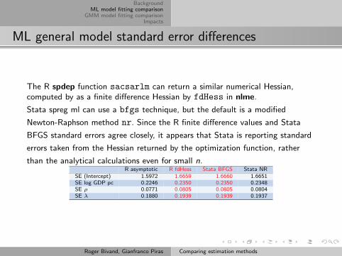
ML general model standard error differences
The R spdep function sacsarlm can return a similar numerical Hessian,computed by as a finite difference Hessian by fdHess in nlme.
Stata spreg ml can use a bfgs technique, but the default is a modified
Newton-Raphson method nr. Since the R finite difference values and Stata
BFGS standard errors agree closely, it appears that Stata is reporting standard
errors taken from the Hessian returned by the optimization function, rather
than the analytical calculations even for small n.R asymptotic R fdHess Stata BFGS Stata NR
SE (Intercept) 1.5972 1.6659 1.6660 1.6651SE log GDP pc 0.2246 0.2350 0.2350 0.2348SE ρ 0.0771 0.0805 0.0805 0.0804SE λ 0.1880 0.1939 0.1939 0.1937
Roger Bivand, Gianfranco Piras Comparing estimation methods
BackgroundML model fitting comparison
GMM model fitting comparisonImpacts
GMM model fitting comparison
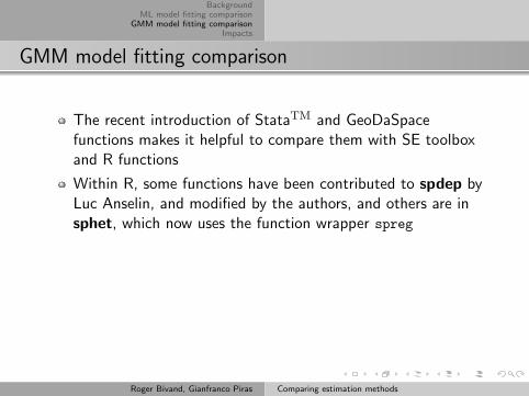
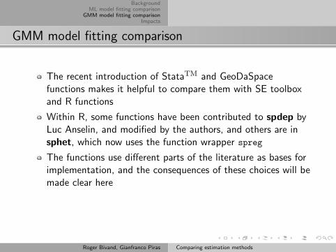
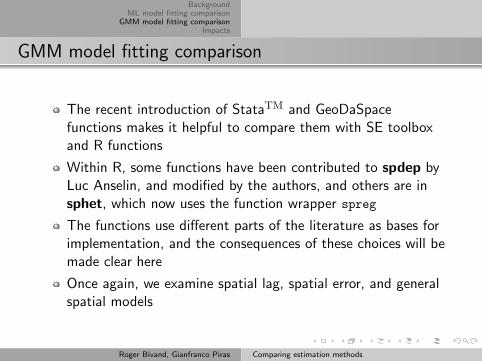
The recent introduction of StataTM and GeoDaSpacefunctions makes it helpful to compare them with SE toolboxand R functions
Within R, some functions have been contributed to spdep byLuc Anselin, and modified by the authors, and others are insphet, which now uses the function wrapper spreg
The functions use different parts of the literature as bases forimplementation, and the consequences of these choices will bemade clear here
Once again, we examine spatial lag, spatial error, and generalspatial models
Roger Bivand, Gianfranco Piras Comparing estimation methods
BackgroundML model fitting comparison
GMM model fitting comparisonImpacts
GMM model fitting comparison
The recent introduction of StataTM and GeoDaSpacefunctions makes it helpful to compare them with SE toolboxand R functions
Within R, some functions have been contributed to spdep byLuc Anselin, and modified by the authors, and others are insphet, which now uses the function wrapper spreg
The functions use different parts of the literature as bases forimplementation, and the consequences of these choices will bemade clear here
Once again, we examine spatial lag, spatial error, and generalspatial models
Roger Bivand, Gianfranco Piras Comparing estimation methods

BackgroundML model fitting comparison
GMM model fitting comparisonImpacts
GMM spatial lag models
Using two stage least squares with Wy instrumented by [WX,WWX], all
the functions yield the same coefficient estimates. In the two R and SE
toolbox functions, the error variance is calculated as σ2 = e′en−k , while in
the other two implementations is simply calculated as e′en :
SE toolbox R spdep R sphet spreg Stata GeoDaSpace(Intercept) -5.7466 -5.7466 -5.7466 -5.7466 -5.7466
(2.4576) (2.4576) (2.4576) (2.4341) (2.4341)log GDP pc 0.9097 0.9097 0.9097 0.9097 0.9097
(0.3783) (0.3783) (0.3783) (0.3747) (0.3747)ρ 0.6370 0.6370 0.6370 0.6370 0.6370
(0.2283) (0.2283) (0.2283) (0.2261) (0.2261)
Roger Bivand, Gianfranco Piras Comparing estimation methods
BackgroundML model fitting comparison
GMM model fitting comparisonImpacts
The heteroskedastic error case I
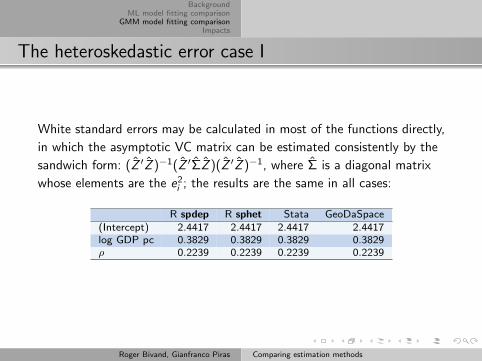
White standard errors may be calculated in most of the functions directly,
in which the asymptotic VC matrix can be estimated consistently by the
sandwich form: (Z ′Z )−1(Z ′ΣZ )(Z ′Z )−1, where Σ is a diagonal matrix
whose elements are the e2i ; the results are the same in all cases:
R spdep R sphet Stata GeoDaSpace(Intercept) 2.4417 2.4417 2.4417 2.4417log GDP pc 0.3829 0.3829 0.3829 0.3829ρ 0.2239 0.2239 0.2239 0.2239
Roger Bivand, Gianfranco Piras Comparing estimation methods

BackgroundML model fitting comparison
GMM model fitting comparisonImpacts
The heteroskedastic error case II
GeoDaSpace and sphet also implement the Kelejian and Prucha (2007)
HAC estimator of the variance covariance matrix. Here we compare
standard error estimates using a Triangular kernel with a variable
bandwidth of the six nearest neighbours. The available options for the
kernel function in R are the Epanechnikov, Triangular, Bisquare, Parzen,
Tukey-Hanning and Quadratic Spectral. The options available in GeoDa
space are the Uniform, Triangular, Epanechnikov, Quartic and Gaussian.
GeoDa space only allows for the implementation of adaptive kernel.
R sphet spreg GeoDaSpace(Intercept) 2.7512 2.7512log GDP pc 0.4445 0.4445ρ 0.2314 0.2314
Roger Bivand, Gianfranco Piras Comparing estimation methods

GMM spatial error models
In the GMM spatial error model, we depend on the first stage residuals,
the implementation of the moment coment conditions, and the tuning of
the optimiser finding the spatial parameter λ, as well as defintions for
finding the standard error of λ. We see that there are three cases, the
first for the SE toolbox, spdep, and GeoDaSpace-2, using the Kelejian
and Prucha (1999) moment conditions (OLS first stage), and the
standard error of λ from Pruch (2004):
SE toolbox R spdep R sphet Stata GeoDaSpace-1 GeoDaSpace-2(Intercept) -7.5798 -7.5798 -7.5858 -8.8787 -7.5664 -7.5798
(3.0403) (3.0403) (3.0319) (3.2603) (3.0788) (3.0403)log GDP pc 1.3993 1.3993 1.4001 1.5688 1.3976 1.3993
(0.3767) (0.3767) (0.3758) (0.4072) (0.3796) (0.3767)λ 0.5621 0.5621 0.5604 0.5586 0.5850 0.5621
(0.1820) (0.1820) (0.0661) (0.0668) (0.0660)
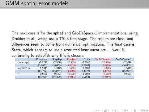
GMM spatial error models
The next case is for the sphet and GeoDaSpace-1 implementations, using
Drukker et al., which use a TSLS first stage. The results are close, and
differences seem to come from numerical optimization. The final case is
Stata, which appears to use a restricted instrument set — work is
continuing to establish why this is chosen:SE toolbox R spdep R sphet Stata GeoDaSpace-1 GeoDaSpace-2
(Intercept) -7.5798 -7.5798 -7.5858 -8.8787 -7.5664 -7.5798(3.0403) (3.0403) (3.0319) (3.2603) (3.0788) (3.0403)
log GDP pc 1.3993 1.3993 1.4001 1.5688 1.3976 1.3993(0.3767) (0.3767) (0.3758) (0.4072) (0.3796) (0.3767)
λ 0.5621 0.5621 0.5604 0.5586 0.5850 0.5621(0.1820) (0.1820) (0.0661) (0.0668) (0.0660)

Heteroskedasticity
Results from sphet and GeoDaSpace are quite similar and the very minor
differences (in the estimated value of the spatial parameter) seem to be
due to differences in the optimizers. This confirms our intuition on the
error model with homoskedastic errors. The standard error results can be
made closer by making the same implementation choices, which differ
slightly with regard to simplifications. Stata differs as before:
R sphet-spreg Stata GeoDaSpace(Intercept) -7.5664 -8.8695 -7.5664
(2.9878) (3.1150) (2.9888)log GDP pc 1.3976 1.5676 1.3976
(0.3613) (0.3664) (0.3614)ρ 0.5731 0.5703 0.5735
(0.0743) (0.0754) (0.0742)

GMM implementations of the general (SARAR) model
There are various implementations of the GMM general model. Some of
them are based on the Kelejian and Prucha (1999) moment conditions
(SE toolbox, gstsls in spdep and GeoDaSpace-2), the others are based
on the Drukker, Egger and Prucha moments conditions (sphet, Stata and
GeoDaSpace-1) with big differences in λ (ML: ρ ≈ 0.78, λ ≈ −0.45):
SE toolbox R spdep R sphet Stata GeoDaSpace-1 GeoDaSpace-2(Intercept) -5.8763 -5.1817 -5.1780 -5.1780 -5.1889 -5.1817
(2.6631) (2.3185) (2.2101) (2.2101) (2.0800) (2.2963)log GDP pc 0.7986 0.8199 0.8193 0.8193 0.8210 0.8199
(0.3556) (0.3600) (0.3314) (0.3314) (0.3255) (0.3566)ρ 0.6938 0.6779 0.6781 0.6781 0.6774 0.6779
(0.2033) (0.2072) (0.1814) (0.1814) (0.1763) (0.2053)λ -0.1596 -0.1596 -0.4095 -0.4095 -0.4748 -0.1596
(0.0363) (0.2502) (0.2502) (0.2224)

The general model under heteroskedasticity
Three implementation are available: one from sphet, one from Stata, and
the one from GeoDaSpace. The results are the same for all of the
implementations. Again, sphet and GeDaSpace have the option of
performing step 1.c from Arraiz et al. Even in this case, the results
match, and, therefore, are not reported.
R sphet-spreg Stata GeoDaSpace(Intercept) -5.1889 -5.1889 -5.1889
(2.2119) (2.2119) (2.2119)log GDP pc 0.8210 0.8210 0.8210
(0.3527) (0.3527) (0.3527)ρ 0.6774 0.6774 0.6774
(0.1845) (0.1845) (0.1845)λ -0.4497 -0.4497 -0.4497
(0.2562) (0.2562) (0.2562)
BackgroundML model fitting comparison
GMM model fitting comparisonImpacts
Interpreting spatial lag, Durbin and general models
It has emerged over time, however, that the spatial dependence inthe parameter ρ feeds back
This feedback comes from the fact that the reduced form model isy = (I− ρW)−1Xβ + (I− ρW)−1ε
In the spatial lag model, ∂yi/∂xjr = ((I− ρW)−1Iβr )ij , where I isthe N × N identity matrix, and (I− ρW)−1 is known to be dense
In the spatial Durbin model, ∂yi/∂xjr = ((I− ρW)−1Iβr −Wθr )ij
Roger Bivand, Gianfranco Piras Comparing estimation methods
BackgroundML model fitting comparison
GMM model fitting comparisonImpacts
Implementing impact measures
The awkward Sr (W) = ((I− ρW)−1Iβr ) matrix term needed tocalculate impact measures for the lag model, andSr (W) = ((I− ρW)−1(Iβr −Wθr )) for the spatial Durbin model,may be approximated using traces of powers of the spatial weightsmatrix as well as analytically
The average direct impacts are represented by the sum of thediagonal elements of the matrix divided by N for each exogenousvariable
The average total impacts are the sum of all matrix elementsdivided by N for each exogenous variable
The average indirect impacts are the differences between the directand total impact vectors
Roger Bivand, Gianfranco Piras Comparing estimation methods
BackgroundML model fitting comparison
GMM model fitting comparisonImpacts
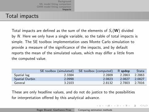
Total impacts
Total impacts are defined as the sum of the elements of Sr (W) divided
by N. Here we only have a single variable, so the table of total impacts is
simple. The SE toolbox implementation uses Monte Carlo simulation to
provide a measure of the significance of the impacts, and by default
reports the mean of the simulated values, which may differ a little from
the computed value.
SE toolbox (simulated) SE toolbox (computed) R spdep StataSpatial lag 2.3384 2.2809 2.2863 2.2863Spatial Durbin 2.0998 2.0823 2.0827 2.0827General 3.2103 2.8132 2.7803 2.7816
These are only headline values, and do not do justice to the possibilities
for interpretation offered by this analytical advance.
Roger Bivand, Gianfranco Piras Comparing estimation methods

Finding total impacts in Stata
In Stata, we use the difference in
predictions from the reduced form model
when incrementing a chosen right-hand
side variable, or even a single
observation on that variable:
. spreg ml democracy x, id(ID) dlmat(W)
. predict y0
. generate x_orig = x
. quietly replace x = x + 1
. predict y1
. generate deltay = y1-y0
. mean deltay
. quietly replace x = x_orig
We can do the same in R, using EXP to
increment the variable in the scope of
the objects:
> EXP <- exp(0)
> form <- formula(democracy ~
+ log((gdp_2002/population) *
+ EXP))
> sldv.lag <- lagsarlm(form, data = sldv,
+ listw = lw)
> p0 <- predict(sldv.lag, newdata = sldv,
+ listw = lw)
> EXP <- exp(1)
> p1 <- predict(sldv.lag, newdata = sldv,
+ listw = lw)
> d <- p1 - p0
> mean(d)
[1] 2.286267
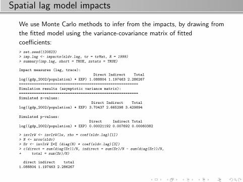
Spatial lag model impacts
We use Monte Carlo methods to infer from the impacts, by drawing from
the fitted model using the variance-covariance matrix of fitted
coefficients:
> set.seed(120823)
> imp.lag <- impacts(sldv.lag, tr = trMat, R = 1999)
> summary(imp.lag, short = TRUE, zstats = TRUE)
Impact measures (lag, trace):
Direct Indirect Total
log((gdp_2002/population) * EXP) 1.088804 1.197463 2.286267
========================================================
Simulation results (asymptotic variance matrix):
========================================================
Simulated z-values:
Direct Indirect Total
log((gdp_2002/population) * EXP) 3.70437 2.665298 3.429894
Simulated p-values:
Direct Indirect Total
log((gdp_2002/population) * EXP) 0.00021192 0.007692 0.00060382
> invIrW <- invIrW(lw, rho = coef(sldv.lag)[1])
> N <- nrow(sldv)
> Sr <- invIrW %*% (diag(N) * coef(sldv.lag)[3])
> c(direct = sum(diag(Sr))/N, indirect = sum(Sr)/N - sum(diag(Sr))/N,
+ total = sum(Sr)/N)
direct indirect total
1.088804 1.197463 2.286267
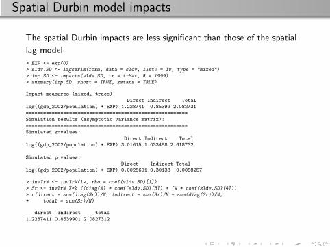
Spatial Durbin model impacts
The spatial Durbin impacts are less significant than those of the spatial
lag model:
> EXP <- exp(0)
> sldv.SD <- lagsarlm(form, data = sldv, listw = lw, type = "mixed")
> imp.SD <- impacts(sldv.SD, tr = trMat, R = 1999)
> summary(imp.SD, short = TRUE, zstats = TRUE)
Impact measures (mixed, trace):
Direct Indirect Total
log((gdp_2002/population) * EXP) 1.228741 0.85399 2.082731
========================================================
Simulation results (asymptotic variance matrix):
========================================================
Simulated z-values:
Direct Indirect Total
log((gdp_2002/population) * EXP) 3.01615 1.033488 2.618732
Simulated p-values:
Direct Indirect Total
log((gdp_2002/population) * EXP) 0.0025601 0.30138 0.0088257
> invIrW <- invIrW(lw, rho = coef(sldv.SD)[1])
> Sr <- invIrW %*% ((diag(N) * coef(sldv.SD)[3]) + (W * coef(sldv.SD)[4]))
> c(direct = sum(diag(Sr))/N, indirect = sum(Sr)/N - sum(diag(Sr))/N,
+ total = sum(Sr)/N)
direct indirect total
1.2287411 0.8539901 2.0827312

General model impacts
The general model impacts are similar to those of the spatial lag model:
> EXP <- exp(0)
> sldv.sac <- sacsarlm(form, data = sldv, listw = lw)
> imp.sac <- impacts(sldv.sac, tr = trMat, R = 1999)
> summary(imp.sac, short = TRUE, zstats = TRUE)
Impact measures (sac, trace):
Direct Indirect Total
log((gdp_2002/population) * EXP) 0.78292 1.997377 2.780297
========================================================
Simulation results (asymptotic variance matrix):
========================================================
Simulated z-values:
Direct Indirect Total
log((gdp_2002/population) * EXP) 3.088464 2.049188 2.476218
Simulated p-values:
Direct Indirect Total
log((gdp_2002/population) * EXP) 0.0020119 0.040444 0.013278
> invIrW <- invIrW(lw, rho = coef(sldv.sac)[1])
> Sr <- invIrW %*% ((diag(N) * coef(sldv.sac)[4]))
> c(direct = sum(diag(Sr))/N, indirect = sum(Sr)/N - sum(diag(Sr))/N,
+ total = sum(Sr)/N)
direct indirect total
0.7829471 1.9986018 2.7815488

BackgroundML model fitting comparison
GMM model fitting comparisonImpacts
Impact measures
At present, there is no provision for measures of impact inOpenGeoDa or Pysal
The total impact (emanating effect, equilibrium effect) can becalculated in Stata, but not broken down into direct andindirect
Only SE toolbox and R provide full support with Monte Carlosimulation for inference
They draw samples from the fitted model using the coefficientvalues and covariance matrix, and present summaries of thesample values
Roger Bivand, Gianfranco Piras Comparing estimation methods

BackgroundML model fitting comparison
GMM model fitting comparisonImpacts
Distributions of general model impact measures
Once one has the samples, it is possible to show how the distributions shift. In
this case, the direct impacts lie further from zero than the coefficient, followed
by indirect impacts even further from zero, with the total impacts shifted
substantially beyond the shape of the distribution of the coefficient:
−2 0 2 4 6 8
0.0
0.5
1.0
1.5
Impacts
Log GDP pc
DirectIndirectTotalCoefficient
Roger Bivand, Gianfranco Piras Comparing estimation methods
BackgroundML model fitting comparison
GMM model fitting comparisonImpacts
Conclusions
In this case, impact measures were not needed, because the LR andHausman tests pointed to the spatial error specification; a recentpaper by Pace and Zhu (2012) points to a enhanced error Durbinmodel as being of promise (it didn’t help here).
We have not considered Bayesian estimation methods, which will becovered in a separate study, where the SE toolbox is the onlyalternative so far, but an R GSoC project has been carried out in2012
The arrival of Stata’s sppack opens up the alternatives a lot, but itsspatial weights are dense or banded, limiting maximum likelihoodestimation to smaller data sets
Estimating models with maximum likelihood for large data sets ispossible in the SE toolbox, OpenGeoDa and R using sparse matrixmethods; GM models are not as limited by the size of data setsgiven care in avoiding handling n × n matrices
Roger Bivand, Gianfranco Piras Comparing estimation methods


