0
Commitments to Save: A Field Experiment in Rural Malawi
Lasse Brune Department of Economics, University of Michigan
Xavier Giné Development Economics Research Group, World Bank and Bureau for Economic Analysis and Development (BREAD)
Jessica Goldberg Ford School of Public Policy and Department of Economics, University of Michigan
Dean Yang
Ford School of Public Policy and Department of Economics, University of Michigan Bureau for Economic Analysis and Development (BREAD) and National Bureau of Economic Research (NBER)
May 2011 Abstract We report the results of a field experiment that randomly assigned smallholder cash crop farmers formal savings accounts. In collaboration with a microfinance institution in Malawi, we tested two primary treatments, offering either: 1) �“ordinary�” accounts, or 2) both ordinary and �“commitment�” accounts. Commitment accounts allowed customers to restrict access to their own funds until a future date of their choosing. A control group was not offered any account but was tracked alongside the treatment groups. Only the commitment treatment had statistically significant effects on subsequent outcomes. The commitment treatment had large positive effects on deposits and withdrawals immediately prior to the next planting season, agricultural input use in that planting, crop sales from the subsequent harvest, and household expenditures in the period after harvest. Across the set of key outcomes, the commitment savings treatment had larger effects than the ordinary savings treatment. Additional evidence suggests that the positive impacts of commitment derive from keeping funds from being shared with one�’s social network. Keywords: savings, commitment, hyperbolic preferences, self-control, sharing norms JEL codes: D03, D91, O16, Q14
Brune: [email protected]. Giné: [email protected]. Goldberg: [email protected]. Yang:
[email protected]. We thank Niall Keleher, Lutamyo Mwamlima and the entire Innovations for Poverty Action staff in Malawi for outstanding field work and data management; Steve Mgwadira and Mathews Kapelemera for their integral contribution to the implementation design and Webster Mbekeani for facilitating access to administrative data; the OIBM management and staff of Kasungu, Mponela and Lilongwe branches for their valuable support throughout the project; and Matt Basilico and Britni Must for excellent research assistance. We are grateful to Oriana Bandiera, Abhijit Banerjee, and seminar participants at the FAI Microfinance Innovation Conference, Ohio State University, the London School of Economics, U. Warwick, and the Institute for Fiscal Studies for helpful comments. We appreciate the consistent and active support of David Rohrbach (World Bank) and of Jake Kendall (Bill and Melinda Gates Foundation). We are grateful for research funding from the World Bank Research Committee and the Bill & Melinda Gates Foundation.

1
1. Introduction
One of the reasons most commonly mentioned by farmers in low-income countries for low
usage of critical inputs for agriculture is �“lack of funds�”. While this may be a catch-all excuse,
the answer is all the more surprising given the high marginal returns to capital among self-
employed individuals in both non-agricultural enterprises (de Mel, McKenzie and Woodruff,
2008) as well as agriculture (Duflo, Kremer and Robinson, 2008).
To alleviate liquidity constraints, many low-income governments and donors have
implemented large-scale input subsidies, but the scale of such programs takes a heavy toll on the
overall government budget (11 percent in 2010 in Malawi) and casts doubt on their
sustainability. Another popular response has been the introduction of microcredit programs. In
2009, the Microcredit Summit estimated that there were more than 3,500 microfinance
institutions around the world with 150 million clients (Daley-Harris 2009). While these outreach
numbers are impressive, microfinance today (and microcredit in particular) is largely devoted to
non-agricultural activities (Morduch 1999; Armendariz de Aghion and Morduch 2005). In
addition, the recent studies that assess the impacts of microcredit programs find benefits that are
more modest than donors and practitioners had previously believed (Kaboski and Townsend,
forthcoming; Banerjee et al. 2010 and Karlan and Zinman, 2010). Finally, when measured
properly, microcredit programs tend to have take-up rates that are much smaller than those of
savings programs. As a result, many donors and academics (for example, Bill and Melinda Gates
Foundation and Robinson, 2001) have emphasized the need for research on the potential
beneficial impacts of formal savings.1
Indeed, low-income individuals have a hard time saving formally, although they do engage
in more expensive and riskier ways to save informally (Rutherford, 2000 and Collins, Morduch,
Rutherford and Ruthven, 2009). The alternatives to formal savings are cash held at home (subject
to theft or fire) investments in durable assets with risky returns (such as livestock), participation
in ROSCAs (rotating savings and credit associations), or use of deposit collectors (such as susu
collectors in West Africa).
1 Burgess and Pande (2005) find that a policy-driven expansion of rural banking reduced poverty in India, and
provide suggestive evidence that deposit mobilization and credit access were intermediating channels.

2
A number of explanations have been advanced for low levels of formal savings in
developing countries. Transaction costs for formal savings may be high for a variety of reasons,
including substantial distances to branches, costly transport, and mistrust towards formal
financial institutions. In addition, financial illiteracy may prevent households from opening
accounts due to a lack of knowledge as to the benefits of formal savings and lack of familiarity
with account-opening procedures.
Formal savings may also be low due to psychological factors, such as impatience (a strong
preference for the present over the future) and issues of self-control (that is, competing
preferences that dictate different actions at different times). There is evidence for both developed
and developing countries that people seek to limit their options in advance in anticipation of self-
control problems in the future, which could be a response on the part of sophisticated or self-
aware hyperbolic discounters (see Ashraf, Karlan, and Yin, 2006 and Duflo, Kremer and
Robinson, 2010).
Yet another potential explanation for low savings levels comes from the observation that in
rural communities individuals are often obliged to share their income with relatives and friends
(see, e.g., Platteau 2000, Maranz 2001; Anderson and Baland (2002); Ligon, Thomas, and
Worall 2002, Baland, Guirkinger and Mali, 2007, Jakiela and Ozier, 2011). This situation may
discourage individuals from accumulating assets or encourage them to spend resources hastily
before income is dissipated through demands from others. People who anticipate pressure to
share cash with others in their social network may spend that money quickly in order to pre-empt
requests for transfers (Goldberg, 2010).
In order to understand the impact of facilitating access to savings accounts and to examine
the importance of these barriers for formal savings, we designed a field experiment among
smallholder cash crop farmers in Malawi. In partnership with a local microfinance institution, we
randomized offers of account-opening and deposit assistance for formal savings accounts.
Because this can be viewed as greatly reducing transaction costs associated with opening and
making initial deposits into bank accounts, this aspect of the intervention can shed light into the
importance of transactions costs.2 In order to test the importance of individual self-control
problems or pressure to share resources with others in the social network, treated farmers were 2 The direct deposit may have helped farmers overcome loss aversion, since farmers with cash in hand may
perceive putting off consumption as a loss (Kahneman and Tversky, 2000).

3
randomly assigned to one of two types of savings interventions. The first group was offered an
�“ordinary�” bank account with standard features. The second group was offered the ordinary
account as well as a �“commitment�” savings account that allowed account holders to request that
funds be frozen until a specified date (e.g., immediately prior to the planting season, so that
funds could be preserved for farm input purchases). Other farmers were assigned to a control
group that was surveyed but not offered assistance with opening either type of savings account.
If offers of commitment accounts have greater impacts than offers of ordinary accounts, then self
control or other-control problems are important.
A sub-experiment was designed to isolate the role of pressure to share with one�’s social
group. Among farmers who were offered the savings treatments, we cross-randomized an
intervention that provided a public signal of individual savings account balances. This public
revelation of balances was done in the context of a raffle in the months immediately prior to the
planting season (when savings would be used for input purchases). Farmers were given a number
of raffle tickets that depended on their savings balances: one raffle ticket was given for each MK
1,000 (about US$7) in savings. In this �“public�” raffle, tickets were distributed in front of other
farming club members. As a result, everyone that attended the raffle distribution meeting was
able to observe the number of raffle tickets received by other members in the club, providing a
signal of individual savings balances.
Because the raffle itself may provide an incentive to save, the design of the experiment
included a �“private raffle�” treatment, identical to the �“public raffle�” but where raffle tickets were
distributed in private, and a �“no raffle�” treatment. If the �“public raffle�” led to lower savings and
less investment in agricultural inputs compared to the �“private raffle�”, it would have been
interpreted as evidence that social pressure to share hinders savings insofar as savings balances
are public. This effect would perhaps be largest among farmers more socially connected, because
they would face pressure to share with more people. If, instead, social comparisons confer
prestige or status, then the �“public raffle�” could have led to higher savings than the �“private
raffle.�” Finally, if the raffle fostered savings, we would expect to find higher balances in clubs
offered any type of raffle compared to clubs in the �“no raffle�” treatment.3
3 One could also argue that the raffle could have made savings salient or that it provided a reminder. Under this
interpretation, the raffle would increase savings (see for example Karlan, McConnell, Mullainathan, Zinman, 2010 and Kast, Meier and Pomeranz, 2010).

4
Our findings are distinguished from those in the existing literature in two ways. First, we are
the first to show impacts of commitment savings offers (as opposed to offers of ordinary
accounts) on important economic outcomes beyond savings, such as inputs into productive
activities, revenues from production, and household expenditures.4 Second, our results are
suggestive that the effects of commitment account offers operate via helping individuals solve
�“other-control�” problems (protecting funds from social network demands), rather than �“self-
control�” problems.
To be specific, the commitment treatment had large positive effects on a range of outcomes
of interest: deposits and withdrawals at our partner institution immediately prior to the next
planting season, land under cultivation (an increase amounting to 9.8% of the control group
mean), agricultural input use in that planting (26.0% increase over the control group mean), crop
output in the subsequent harvest (21.9% increase), and household expenditures in the months
immediately after harvest (17.4% increase). By contrast, ordinary treatment effects are uniformly
smaller than those of the commitment treatment, and are never statistically significantly different
from zero. A joint hypothesis test finds that the impact of the commitment account offer on the
set of key agricultural and expenditure outcomes is statistically significantly larger than the
effect of the ordinary account offer.
Patterns of heterogeneity in take-up and treatment effects suggest that the positive impacts
of commitment derive from keeping funds from one�’s social network. The first piece of evidence
is the fact that the vast majority of the commitment treatment�’s impact on amounts saved (91%)
was on savings in ordinary as opposed to commitment accounts, and that the funds saved in
commitment accounts were about an order of magnitude smaller than the commitment
treatment�’s impact on input use on the farm. Clearly, the commitment treatment did not have its
effect on input use via �“tying the hands�” of farmers in the months prior to planting time. Rather,
it is likely that the existence of the accounts simply allowed farmers to credibly claim that their
funds were inaccessible when faced with social network demands. This is consistent with
commitment savings accounts helping farmers address an �“other-control�” problem rather than a
�“self-control�” problem.
4 As a follow-up to Ashraf, Karlan, and Yin (2006), Ashraf, Karlan, and Yin (2010) show impacts of
commitment account offers on female empowerment in the same Philippine experimental sample.
5
In addition, contrary to Ashraf, Karlan, and Yin (2006) we find no evidence that take-up or
impact of commitment accounts is related to baseline measures of hyperbolic preferences.
Instead, the impacts of the commitment treatment are larger for households with higher assets at
baseline. This may reflect the fact that higher-asset households are more likely to face social
network demands to share resources.
The results from the cross-randomized public and private raffle treatments are inconclusive.
Effects of either type of raffle are mostly not statistically significantly different from zero, and
the few statistically significant coefficients are inconsistently signed across regressions. For this
reason we focus this paper�’s attention on interpreting the effects of the �“no raffle�” savings
treatments.
This paper contributes to the burgeoning literature on the effects of formal savings accounts
and in this sense is related to the field experiments of Dupas and Robinson (2010) and Atkinson
et al. (2010). Dupas and Robinson (2010) offer ordinary savings accounts with de facto negative
interest rates to female Kenyan urban market sellers, finding positive impacts on investment and
income. In this paper, by contrast, we explicitly test whether impacts of commitment savings
offers are larger than impacts of ordinary savings offers. We also use a very different sample,
(mostly) male farmers in rural Malawi. Atkinson et al. (2010) offer microcredit borrowers in
Guatemala savings accounts with different features, including reminders about a monthly
commitment to save and a default of 10% of loan repayment as a suggested monthly savings
target. They find that both features increase savings balances substantially. However, they use
administrative records from the lender which restricts the number of observable outcomes and
limits analysis of the mechanisms that lead to changes in savings behavior. Our paper is also
related to Dupas and Robinson (2011) in seeking to understand the relative importance of various
barriers to savings. Dupas and Robinson (2011) do so in the context of ROSCAs, while we
provide formal savings products.
The remainder of this paper is organized as follows. Section 2 explains the study design and
briefly describes the characteristics of the sample. Section 3 explains the estimation strategy.
Section 4 presents the main empirical results. Section 5 discusses heterogeneous effects and the
mechanisms through which savings accounts may have affected savings and other outcomes.
Section 6 concludes.

6
2. Experimental design and survey data
The experiment was a collaborative effort of Opportunity International Bank of Malawi
(OIBM), Alliance One, Limbe Leaf, the University of Michigan and the World Bank.
Opportunity International is a private microfinance institution operating in 24 countries that
offers savings and credit products. Alliance One and Limbe Leaf are two large private agri-
business companies that offer extension services and high-quality inputs to smallholder farmers
via an out-grower tobacco scheme.5 Farmers in the study were organized by the tobacco
companies into clubs of 10-15 members and all had group liability production loans from OIBM
prior to enrollment in the study.
Table 1 presents summary statistics of baseline household and farmer club characteristics.
All variables expressed in money terms are in Malawi Kwacha (MK145/USD during the study
period). Baseline survey respondents own an average of 4.7 acres of land and are mostly male
(only six percent were female). Respondents are on average 45 years old. They have an average
of 5.5 years of formal education, and have low levels of financial literacy: 42% of respondents
were able to compute 10% of 10,000, 63% were able to divide MK 20,000 by 5 and only 27%
can apply a yearly interest rate of 10% to an initial balance to compute the total savings balance
after a year.
Sixty three percent of farmers at baseline had an account with a formal bank (mostly with
OIBM).6 The average reported savings balance at the time of the baseline in bank accounts was
MK 2,083 (USD 14), with an additional MK 1,244 (USD 9) saved in the form of cash at home.
Figure 1 presents the timing of the experiment with reference to the Malawian agricultural
season. The baseline survey and interventions were administered in April and May 2009,
immediately before the 2009 harvest.
Financial Education Session
5 Tobacco is central to the Malawian economy, as it is the country�’s main cash crop. About 70% of the
country�’s foreign exchange earnings come from tobacco sales, and a large share of the labor force works in tobacco and related industries.
6 This number includes a number of �“payroll�” accounts opened in a previous season by OIBM and one of the tobacco buyer companies as a payment system for crop proceeds, and which do not actually allow for savings accumulation. Our baseline survey unfortunately did not properly distinguish between these two types of accounts.

7
After the baseline was administered, all clubs (treatment as well as control) were
administered a financial education session intended to explain the benefits of formal savings
accounts, teach them the elements of budgeting, and in particular to encourage farmers to set
aside funds intended from immediate consumption from funds needed for the future (such as for
school fees or agricultural inputs). The full script of the financial education session can be found
in Appendix A.
Because we provided this financial education to our control group as well, we can estimate
neither the impact of the ordinary and commitment treatments without such financial education,
nor the impact of the financial education alone. We provided the financial education session to
all study participants so that any effects of the ordinary or commitment treatments could be
clearly interpreted as due to the provision of the financial products themselves, rather than due to
any financial education (for example, strategies for improved budgeting) implicitly provided
during the product offer.
Ordinary and Commitment Treatments
Farmers were randomly assigned to one of three savings treatment conditions. The first
experimental group was the control group and only received the financial education session
described above.
Implementation of the savings treatment took advantage of the existing system of
channeling crop sale proceeds into OIBM bank accounts. Production loans provided by OIBM
were repaid directly to the lender via garnishing of farmers�’ tobacco sale proceeds. In the control
group, the process was as follows. At harvest, farmers sold their tobacco to the company that
organized them at the price prevailing on Malawi�’s centralized tobacco auction floor. The
proceeds from the sale were then electronically transferred to OIBM, which deducted the loan
repayment (plus fees and surcharges) of all borrowers in the club, and then credited the
remaining balance to a club account at OIBM. Club members authorized to access the club
account (usually the chairman or the treasurer) came to OIBM branches and withdraw the funds
in cash. Farmers then divided up the cash within the club. In the treatment groups, farmers were
offered the opportunity to have their crop sale proceeds channeled directly into individual
savings accounts, as we now describe.
Farmers in the savings treatment groups were given the same financial education session
provided to the control group but in addition were given account opening assistance and were

8
offered the opportunity to have their harvest proceeds (net of loan repayment) directly deposited
into individual accounts in their names (see Figure 2 for a schematic illustration of money
flows). After their crop was sold, farmers traveled to the closest OIBM branch to confirm that
positive proceeds net of repayment were available at the club level. Authorized members of the
clubs (often together with other club members) then filled out a sheet specifying the division of
the total amount between farmers. Depending on whether a club member had opted for the
individual accounts or not, funds were then either transferred to the individual�’s account(s) or
paid out in cash.
There were two savings treatment conditions. In the first, farmers were offered only an
ordinary savings account (the �“ordinary�” treatment). In the second, farmers were offered both an
ordinary and a commitment savings account (the �“commitment�” treatment). Farmers in the
control group and the �“ordinary�” treatment group who may have learned about and requested
commitment accounts were not denied those accounts, but they were not prompted to open them,
either.7
An ordinary savings account is a regular OIBM savings account with an annual interest rate
of 2.5%. The commitment savings account has the same interest rate but allows farmers to
specify an amount and a �“release date�” when the bank would allow access to the funds.
Farmers who chose to open a commitment savings account were also required to have an
ordinary account where uncommitted funds would be deposited. Although neither of the two
accounts was specifically labeled, one could argue that having two separate accounts might
facilitate mental accounting and help achieve two different savings goals (Thaler, 1990). We
return to this interpretation when we discuss the results in Section 4.
During the account opening process, farmers stated how much they wanted in the ordinary
and commitment savings accounts after their tobacco crops would be sold. For example, if a
farmer stated that that he wanted MK 5,000 in an ordinary account and MK 10,000 in a
commitment savings account, funds would first be deposited into the ordinary account, then into
7 Among farmers in the control group, nobody requested an ordinary or a commitment account during the
savings training at baseline. According to OIBM administrative records, eight farmers in the control group had commitment accounts by the end of October 2009 (opened without our assistance or encouragement), but none of these had any transactions in the accounts.

9
the commitment savings account, with any remainder being deposited back into the ordinary
account.8
Raffle Treatments
To study the impact of public information on savings and investment behavior, we
implemented a cross-cutting randomization of a savings-linked raffle. Participants in each of our
two savings treatments were randomly assigned to one of three savings-linked raffle conditions.
These raffles provided a mechanism for randomizing information about each other�’s savings
balances. We distributed tickets for a raffle to win a bicycle, where the number of tickets each
participant received was determined by his savings balance as of pre-announced dates. Every
MK 1,000 saved with OIBM (in total across ordinary and commitment savings accounts) entitled
a participant to one raffle ticket. Tickets were distributed twice. The first distribution took place
in early September, and was based on savings as of August 19. The second distribution took
place in November, and was based on savings as of October 22. By varying the way in which
tickets were distributed, we sought to manipulate the information that club members had about
each other�’s savings. One third of clubs that was assigned to either ordinary or commitment
savings accounts was randomly determined to be ineligible to receive raffle tickets (and was not
told about the raffle). Another one third of clubs with savings accounts was randomly selected to
have raffle tickets distributed privately. The final third of clubs with savings accounts was
randomly selected for public distribution of raffle tickets. In these clubs, each participant�’s name
and the number of tickets he received was announced to everyone that attended the raffle
meeting.
Because of the simple formula for determining the number of tickets, farmers in clubs
where tickets were distributed publicly could easily estimate how much other members of the
club had saved. Private distribution of tickets, though, did not reveal information about
individuals�’ account balances. The raffle scheme was explained to participants at the time of the
baseline survey using a simulation. Members were first given hypothetical balances, and then
given raffle tickets in a manner that corresponded to the distribution mechanism for the treatment
8 Notice that members could have revised the initial allocation of funds made during the initial account
opening process when they visited the bank after the crop sale. However, we find no evidence of this behavior in practice (analysis not reported) using data from the club funds allocation sheets.
10
condition to which the club was assigned. In clubs assigned to private distribution, members
were called up one by one and given tickets in private (out of sight of other club members). In
clubs assigned to public distribution, members were called up and their number of tickets was
announced to the group.
Thus, the final design of the project includes seven treatment conditions: a pure control
condition without savings account offers or raffles; ordinary savings accounts with no raffles,
with private distribution of raffle tickets, and with public distribution of raffle tickets; and
commitment savings accounts with no raffles, with private distribution of raffle tickets, and with
public distribution of raffle tickets (see Table 2).
The randomization was carried out at the club level. The list of tobacco clubs in central
Malawi (all of which had existing production loans with OIBM) was provided by OIBM in
cooperation with the two tobacco buyer companies. Prior to randomization, treatment clubs were
stratified by location9, tobacco type (burley, flue-cured or dark-fire) and week of scheduled
interview. The stratification of treatment assignment resulted in 19 distinct location/tobacco-
type/week stratification cells.
The sample for analysis consists of 299 clubs with 3,150 farmers surveyed at baseline, and
298 clubs with 2,835 farmers surveyed at endline.10 Attrition from the baseline to the endline
survey was 10.0% and does not vary substantially by treatment status (as shown in Appendix
Table 1). While attrition is uncorrelated with treatment assignment for 5 out of the 6 treatment
groups, farmers in the ordinary / private raffle treatment group are about 3% less likely to attrit
from baseline to endline survey, compared to the control group, and this difference is statistically
significant at the 10% level (p-value 0.085 in the specification with full baseline controls). Since
the focus of the paper is on the impacts of ordinary and commitment account treatments without
raffle, and the difference is very small, we do not view this as an important concern. 9 �“Locations�” are the tobacco buying companies�’ geographically-defined administrative units within which
extension services and contract buying activities are coordinated. 10 60 clubs in two locations had to be excluded from the sample because of serious implementation
irregularities. Clubs in Kasungu Central were discovered to contain substantial numbers of �“ghost�” (nonexistent) club members and served as vehicles for larger landowners to fraudulently obtain very large loans from our partner institution; survey data collected for these individuals is thus likely to be fictitious and therefore unusable. Clubs in Mndolera were excluded because of clerical and communications errors that led to ambiguity in treatment assignment. In the two locations subject to these issues, we excluded all clubs (amounting to the three affected stratification cells) from the sample. Because entire stratification cells were excluded, inference among the remaining stratification cells is not subject to selection bias. As it turns out, regressions that do include these 60 clubs yield qualitatively very similar results with similar statistical significance levels.

11
Balance of baseline characteristics across treatment conditions
To examine whether randomization across treatments achieved balance in pre-treatment
characteristics, Table 3 presents the differences in means of 17 baseline variables for the six
treatment groups vis-a-vis the control group. For statistical inference about the differences in
means we estimate the following regression for farmer i in club j for each baseline variable Yij:
(1) Yij = + 1Ordinaryj + 2Ord_PrivRafj + 3Ord_PubRafj
+ 4Commitmentj + 5Com_PrivRafj + 6Com_PubRafj + �’Sij + ij
Ordinaryi is an indicator variable for assignment to the ordinary treatment and Commitmenti
is an indicator variable for assignment to the commitment treatment. Ord_PrivRafj and
Ord_PubRafj are indicator variables for the assignment to the ordinary treatment and the private
or public raffle treatment, respectively. Com_PrivRafj and Com_PubRafj are defined similarly,
indicating assignment to the commitment treatment and either the private or the public raffle
treatment condition. These indicators are essentially interactions of Ordinaryj and Commitmentj,
respectively, with variables indicating assignment to the private or public raffle treatment
conditions. Sij is a vector that includes stratification cell dummies. ij is a mean-zero error and
because the unit of randomization is the club, standard errors are clustered at this level (Moulton
1986).
Coefficients 1 and 4 measure the difference in means of the dependent variable between
the ordinary treatment and the commitment treatment, respectively (without additional raffle
treatments) vis-à-vis the control group. The difference ( 4- 1) represents the difference in means
between the ordinary treatment and the commitment treatment (each without layered-on raffle
treatments). The coefficient 2 measures the difference in means between the ordinary treatment
group without raffle and the ordinary treatment combined with additional private raffle
treatment. Similarly, 3 measures the difference in means between the ordinary treatment group
without raffle and the ordinary treatment combined with additional public raffle treatment. The
coefficients 5 and 6 measure the same differences in means for the commitment treatment
groups.
With a few exceptions, baseline variables for the ordinary and commitment (without raffle)
treatment groups are quite balanced with the control group. The exceptions are that individuals in
the ordinary group are more likely to be female (column 1), less likely to be married (column 2),
and less likely to be �“patient now, impatient later�” (column 14); and individuals in the

12
commitment group are more likely to be female. Overall, however, for both the ordinary and
commitment (no raffle) groups we cannot reject the null that means of all 17 baseline variables
are jointly equal to those in the control group (see p-values of F-tests at the bottom of Table 3).
The situation is similar for the coefficients on the interactions between the savings and raffle
treatments �– most outcomes are balanced vis-à-vis the corresponding �“no raffle�” savings
treatment, with a scattering of statistically significant differences that are not too different from
what would likely have arisen by chance. Again, for none of the raffle sub-treatments can we
reject the null at conventional levels that the full set of baseline variables is jointly equal to the
mean for the corresponding �“no raffle�” treatment.
To alleviate any concern that baseline imbalance may be driving our results, we follow
Bruhn and McKenzie (2009) and include the full set of baseline characteristics in Table 3 as
controls in our main regressions, alongside the stratification cell fixed effects.11
3. Estimation strategy
A number of dependent variables are of interest, such as deposits and withdrawals prior to
the next planting season, inputs used in the next planting, crop output and sales in the next
planting, and household expenditures after the next harvest.
To estimate the impact of the treatments we estimate the following regression analogous to
equation 1 above:
(2) Yij = + 1Ordinaryj + 2Ord_PrivRafj + 3Ord_PubRafj
+ 4Commitmentj + 5Com_PrivRafj + 6Com_PubRafj + �’Xij + ij
Yij is the dependent variable of interest for farmer i in club j. The savings treatment
indicators Ordinaryi and Commitmenti and the respective interactions with the raffle treatment
indicators Ord_PrivRafj, Ord_PubRafj\, Com_PrivRafj and Com_PubRafj are defined as in
equation 1. Xij is a vector that includes stratification cell dummies and control variables
measured in the baseline survey, prior to treatment (the 17 baseline variables in Table 3).
Following closely the interpretation of equation 1 above, the coefficients on the treatment
indicators ( 1 and 4) reflect the impact on the dependent variable of the ordinary treatment and
11 Results turn out to be very similar when only stratification cell fixed effects are included. See Appendix
Tables 2, 3 and 4.

13
the commitment treatments, respectively, without additional raffle treatments vis-à-vis the
control group, as well as the differential impacts of the savings treatments when combined with
the private raffle ( 2 and 3) or public raffle treatments ( 5 and 6).
We focus on intent-to-treat (ITT) estimates because not every club member offered account
opening assistance decided to open the account. We do not report average treatment on the
treated (TOT) estimates. It is plausible that members without accounts are influenced by the
training script itself or by members who do open accounts in the same club, either of which
would violate SUTVA (Rubin, 1974).
4. Empirical results: impact of treatments
To understand the impacts of access to formal savings, we first study the extent to which
funds flowed into and out of the savings accounts in the pre-planting and planting periods. Then
we examine impacts on agricultural inputs, farm output, household expenditures and other
household outcomes.
A. Savings transactions (deposits and withdrawals)
Table 4 presents regression results from estimation of equation 1. The first column presents
results in which the dependent variable is an indicator variable for whether any transfers were
made from the club account to the farmer�’s individual account after the group loan had been
repaid. Columns 2 to 8 present results for three types of savings behaviors: deposits (separately
for ordinary, commitment and other accounts, as well as the sum across all accounts), sum of
withdrawals, and net deposits into OIBM accounts in different time periods. The �“pre-planting�”
period, from March 2009 to October 2009, is the period when funds are accumulated from the
previous season�’s harvest in preparation for purchasing inputs for the 2009-2010 growing
season. The �“planting�” period, from November 2009 to April 2010, includes the time of year
when farmers purchase inputs and tend their crops. It lasts until the 2010 harvest. These data are
obtained from OIBM administrative records.
Results from column 1 show that while none of the farmers in the control group transferred
money via direct deposit into an OIBM account (since they were not offered direct deposit or
account opening assistance), 16% of farmers in the ordinary account, no raffle treatment did

14
transfer money. This percentage is somewhat larger at 21% for farmers in the commitment
savings treatment without raffle. There are no statistically significant effects of either the public
or private raffle on farmers assigned to either of the savings treatment conditions. Farmers in
each of the six savings treatment conditions had significantly higher deposits (at the 1%
significance level) than farmers in the control group.
Although most farmers offered the ordinary and commitment accounts expressed interest
during the baseline, by late October 2009 only about 29% had activated the ordinary account by
paying the MK500 account opening fee at the branch.12,13
Farmers�’ stated intentions for savings in the commitment accounts focused mostly on
farming inputs. Over 70% respondents who opened commitment accounts mentioned fertilizer or
other inputs among their top three savings goals for the account. Other, much less mentioned
intended uses include saving for home improvement and school fees.
Figure 3 shows a histogram of release dates (dates when funds would be �“unlocked�” and
transferred into ordinary accounts) that farmers chose during account opening. In accordance
with their stated savings goals, 60% of farmers chose release dates in the month of October to
December when most input purchases occur, immediately prior to or at the start of the planting
season. Some farmers also chose to have access to the funds in January and February, during the
lean or �“hungry�” season.
Turning to deposits into saving accounts, most notably, both ordinary and commitment
treatments led to higher total deposits (column 5) as well as higher total withdrawals (column 6)
during the pre-planting period compared to the control group. Coefficients on both types of
savings treatments are positive and statistically significantly different from zero for deposits
(column 5), and negative and statistically significantly different from zero for withdrawals
(column 6). The coefficient on the commitment treatment without raffle is virtually the same as
the coefficient on the ordinary treatment without raffle.
By and large, public distribution of raffle tickets did not appear to affect savings behavior.
An anomalous result is that among those farmers assigned to the ordinary savings account
12 We fail to detect significant differences in account take-up between ordinary and commitment treatments
and between the raffle and the �“no raffle�” treatment conditions. 13 One of the reasons why actual take-up was below 30% had to do with the low price for one of the most
common types of tobacco (burley). The price was about 25% lower during the 2009 season compared to 2008. As a result, several clubs were unable to fully repay their club loans, and so no proceeds were left to be paid to farmers.

15
treatment, the private raffle led to lower deposits and lower withdrawals when compared to
farmers in the ordinary (no raffle) treatment. We have no good explanation for this result, and
believe it may be simply due to sampling variation.14
To understand the savings effects further, we divide total savings into ordinary savings
(column 2), commitment savings (column 3) and savings in other accounts (column 4). It is clear
that most of the funds are deposited into the ordinary account, even among farmers also offered a
commitment savings account. For this group, however, as expected, balances in the commitment
account were positive and statistically different from balances in the control group (with a mean
of zero). Since average commitment-account balances for farmers in the commitment group were
quite low, explanations of the impacts based on mental accounting or self-control seem
implausible. We elaborate this point in greater detail in Section 6.
Finally, we turn to net deposits (column 7), defined as the difference between deposits and
withdrawals across all accounts during the pre-planting period. The commitment savings, no
raffle treatment led to a small and statistically significant increase on net deposits, while the
effect of the ordinary account without raffle was not statistically different from zero. The
difference in coefficients between ordinary and commitment treatments is not statistically
significantly different from zero, however. There is no differential effect of either raffle.
In the last column of Table 4 we examine availability of funds in the savings accounts
during the planting season, November 2009 to April 2010. This period includes the February to
March 2010 �“hungry�” season when households may have used up the maize stored from the
previous season�’s harvest and have not yet harvested crops or received payments for the 2010
harvest.
Column 8 indicates that the commitment treatment groups �– on net �– withdrew more funds
during the planting season whereas there is no large or statistically significant effect of the
ordinary treatment on net transactions during this time period. This result suggests that the
commitment treatment allowed farmers to save funds for the annual lean or �“hungry�” season.
While we do not have consumption data for this period, these withdrawals may have led to
smoother hungry season consumption for the households of farmers in the commitment group.
14 In subsequent results tables for other dependent variables, this negative coefficient on the �“Ordinary x
Private Raffle�” variable does not reappear, which we see as further evidence that this result is anomalous.

16
B. Inputs, crop sales, and expenditures
We now turn to impacts of the treatments on inputs, crop sales, and expenditures in Table 5.
Across the seven dependent variables the commitment (no raffle) treatment has large positive
and statistically significant impacts. In comparison, the coefficients on the ordinary savings
treatment are never statistically significantly different from zero at conventional levels. While
the coefficients are also mostly positive they are substantially smaller in magnitude relative to
the commitment treatment coefficients. For several of the outcomes, discussed below, we can
reject that the coefficients on the ordinary and commitment treatment are equal. The effects of
either the public or private raffle are generally not statistically significant and when the effects
are significant, there is no consistent pattern across outcomes. This is puzzling but suggests that
we should not over-interpret individual coefficients on the raffle variables.
The first two columns of the table reveal that the commitment (no raffle) treatment had a
large positive and statistically significant effect on both land under cultivation and the total value
of inputs used (which include seed, fertilizer, pesticides, hired labor, transport and firewood for
curing) in the late-2009 planting. Farmers in the commitment group cultivated on average 0.42
more acres of land than the control group (which had 4.3 acres of land under cultivation). The
commitment coefficient is statistically significantly different (p-value 0.057) from the ordinary
coefficient of 0.05 which in turn is not statistically different from zero. Compared to MK59,754
in inputs used by control group farmers on average, commitment treatment farmers used
MK15,551 (or 26%) more. By contrast, while the coefficient on the ordinary (no raffle)
treatment is also positive, it is only about half the magnitude of the commitment (no raffle)
treatment coefficient and it is not statistically significantly different from zero. The difference in
the coefficients on the two treatments, however, is not statistically different from zero at
conventional levels.
Columns 3, 4 and 5 indicate that the larger input use caused by the commitment treatment
resulted in higher total crop output in the 2010 harvest. The coefficient on the commitment
treatment is large and statistically significantly different from zero at the 10% level for proceeds
from crop sales (column 3) and for the value of crop not sold (column 4). The coefficient on the
commitment (no raffle) treatment on the value of crop sold and unsold output (column 5, the sum
of the dependent variables in the previous two columns) is statistically significantly different
from zero at the 1% level. The increase in total value of crop output (MK 33,443) amounts to

17
22% of mean sales in the control group. The coefficient on the ordinary (no raffle) treatment in
column 5 is also positive but its magnitude is only about 20% of that on the commitment
treatment, and is not statistically significantly different from zero. The difference between the
ordinary (no raffle) and commitment (no raffle) coefficients in column 5 is statistically different
from zero at the 10% level (p-value 0.076).
Column 6 of Table 5 shows the impact of the experimental treatments on farm profits,
defined as the difference between the total value of crop output (dependent variable of column 5)
and the total value of inputs used (dependent variable of column 2). The coefficient on the
commitment treatment is large but only marginally significant (p-value 0.13). The coefficient for
the ordinary account is small and not statistically significant, and the difference vis-a-vis the
commitment account is marginally significant (p-value 0.118).
Column 7 examines the impact of the treatments on total household expenditures in the
endline (post-harvest) survey. The commitment (no raffle) treatment coefficient is positive and
statistically significantly different from zero at the 5% level, while the coefficient on the ordinary
(no raffle) treatment is substantially smaller and not statistically significantly different from zero.
The commitment (no raffle) treatment effect represents a 17% increase total expenditures over
the last 30 days compared to the control group.
In order to examine further whether the commitment accounts treatment had a differential
impact vis-a-vis the ordinary accounts across the full set of outcomes in Table 5, we follow
Kling, Liebman and Katz (2007) and present p-values of two F-tests at the bottom of Table 5 that
are based on seemingly unrelated regressions (SUR) estimation. We simultaneously estimate
equation 1 with the dependent variables of column 1, 2, 5 and 7.15 We cannot reject that the
coefficient on the ordinary (no raffle) treatment is jointly equal to zero across the four
regressions (p-value 0.283). In contrast, we do reject that the coefficient on the ordinary (no
raffle) treatment equals the coefficient on commitment (no raffle) treatment (p-value 0.061).
So far we have focused on the results for treatment groups without the raffle. As mentioned
15 We restrict attention to just the regressions for the four outcomes in columns 1, 2, 5, and 7 of Table 5
because the other outcomes in the table do not provide additional substantive information. The dependent variable in column 5 (value of crop output, sold and not sold) is constructed as the sum of the dependent variables in columns 3 (proceeds from crop sales) and 4 (value of crop not sold), while the dependent variable in column 6 (farm profit) is constructed as the dependent variable in column 5 (value of crop output, sold and not sold) minus the dependent variable in column 2 (total value of inputs).
18
before, the pattern of coefficients for the differences of private or public raffle vs. no raffle
treatments is largely inconsistent between ordinary and commitment treatments, and as such we
find the results to be inconclusive. For several outcomes, the effect of the ordinary (public raffle)
treatment does seem to be more positive than the effect of the ordinary (no raffle) treatment. The
p-values at the bottom of the table also indicate positive overall effects of the ordinary (public
raffle) treatment compared to the control group. These differences do not appear to be driven by
baseline imbalance, and may simply reflect sampling variation.
C. Other outcomes
Table 6 presents the regression results on the impacts of the treatments on household size,
transfers to and from the social network, and demand for fixed deposit accounts, measured at the
endline survey.
Column 1 shows that the intervention had no effect on household size. This implies that the
impacts presented in Table 5 are driven by changes in agricultural decisions and outcomes rather
than changes in household composition. The fact that household size does not change also means
that the change in household consumption found in Table 5 can be more readily interpreted as
reflecting improved wellbeing in the household.
We are particularly interested in transfers sent and received because one of the barriers to
savings may be the inability to resist demands from the social network. Although net balances in
the commitment accounts were small, the existence of the account may have provided an excuse
to turn down requests for assistance from the social network by claiming that their savings were
inaccessible.
In columns 2, 3 and 4 of Table 6 we examine the sums of transfers made, transfers received
and net transfers over the last twelve months. In order to explain the higher input use for
commitment group farmers, additional availability of resources is most relevant during the pre-
planting period. Thus, we present results in columns 5, 6 and 7 from regressions with dependent
variables similar to those in columns 2 to 4 but with the sums of transfers restricted to categories
in which the biggest gift was made before or during October 2009 (see Appendix B for further
details of the variable definitions).
We find no evidence of reduced net transfers for the commitment (no raffle) treatment. If
anything, there is a small positive, weakly statistically significant effect on net transfers made

19
(column 4). Results are qualitatively similar for the set of restricted transfer variables (columns 5
to 7). The effect of the commitment (no raffle) treatment on net transfers in column 7 is
somewhat smaller in magnitude compared to its �“unrestricted�” transfers equivalent in column 4
(but more strongly statistically significant).
Though we do not find evidence that commitment savings accounts directly reduced
transfers to other members of the social network, the accounts may have helped farmers shield
their resources from another manifestation of social pressure to share. Individuals who know
they will be subject to demands from others in their social network can prevent others from
claiming their money by spending it preemptively. Rapidly consuming income makes it
unavailable to others; it is consistent with signaling a high marginal utility of consumption in a
model where income is taxed and redistributed from those with low marginal utility of
consumption to high marginal utility of consumption. Goldberg (2010) found support for such a
model in an experiment that demonstrated that Malawian cash crop farmers who received money
in public settings spent significantly more of that money immediately than farmers who received
money in private settings. In this project, we do not have the high-frequency consumption data
necessary to test whether farmers with commitment savings accounts were less likely to engage
in hasty consumption than farmers without such accounts. However, a reduction in sub-
optimally timed consumption is a channel through which offers of commitment accounts could
have led to increased use of inputs and improvements in output, profits, and household
expenditures.
Lastly, we study subsequent demand for fixed deposit accounts (column 8) at the time of the
endline survey. Fixed deposit accounts in Malawi typically have a duration of three or six
months. The client makes an initial one-time deposit of pre-specified amounts, typically in
multiples of MK10,000. During the three- or six-month duration the client cannot make a
withdrawal from the fixed deposit account and also cannot increase the savings balance.
Interestingly, we find that ownership of fixed deposit accounts is six percentage points
higher and significant at 1% level in the commitment (no raffle) group, and three percentage
points higher in the ordinary (no raffle) group (significant at the 5% level) compared to the
control group. The results suggest that our treatments, particularly the commitment (no raffle)
treatment, valued savings products with commitment features. The difference in effects between
ordinary and commitment, however, is not statistically significant.

20
5. Heterogeneous effects
Commitment savings accounts may have caused higher deposits, greater availability of
funds at planting time, and higher expenditures on agricultural inputs by helping farmers manage
their own self-control problems, or by helping them manage demands from others in their social
networks. In this section we shed light indirectly on the different mechanisms through which
commitment savings accounts may have operated.
Our approach is to examine the extent to which treatment effects are heterogeneous vis-à-vis
particular baseline variables. We estimate regression equations of the following form:
(3) Yij = + 1(Channelij*Ordinaryj)
+ 2(Channelij*Ord_PrivRafj + 3(Channelij*Ord_PubRafj)
+ 4(Channelij*Commitmentj)
+ 5(Channelij*Com_PrivRafj)+ 6(Channelij*Com_PubRafj)
+ �’Xij + ij
where Channelij is a vector of individual characteristics including an indicator for having a
hyperbolic discount rate, a measure of net transfers to others in the year before the baseline
survey, and an index for baseline level of assets. Other right-hand-side variables include, as
before, the baseline controls and stratification cell fixed effects.
We present results from this exercise in two sets of regressions in Table 7. In each set of
regressions we show effects on total deposits during the pre-planting season (columns 1 and 4),
on total value of farm inputs (columns 2 and 5), and on output (columns 3 and 6) The main
effects for the baseline variables that are interacted with the treatment indicators are all included
in the set of baseline controls.
We focus our discussion on the coefficients on the ordinary (no raffle) and commitment (no
raffle) treatments, since in Tables 4, 5 and 6 we found that the effects of the raffle treatments
were inconclusive.
The first set of columns shows results from regressions with treatment indicators interacted
with net transfers made to the social network over the last 12 months as of the date of the
baseline interview and interactions with an indicator for whether the respondent is classified as
exhibiting hyperbolic time preferences based on a series of hypothetical questions at baseline.
21
The second set of columns has results from regressions that include additional interactions with
an indicator for the �“Patient now, impatient later�” time preference reversal, an index for asset
ownership and years of education.
In our baseline survey, we ask respondents to make hypothetical trade-offs between
receiving some money sooner, or more money later. These questions are designed to be
analogous to the questions capturing time-preference reversals used by Ashraf, Karlan, and Yin
(2006). Survey respondents are asked whether they prefer MK100 now or MK110 one month
from now. Respondents who prefer MK100 now are then asked to choose between MK100 from
now and MK130 one month from now. The questions continue, with the value of the
hypothetical payment in one month increasing from MK130 to MK150, MK200, and MK250,
thus soliciting bounds on the discount rate for which the respondent is willing to wait one month
to receive money. Later in the survey, after completing unrelated modules, we ask the same
questions over a different time frame: 12 months from now compared to 13 months from now.
Individuals who are more patient with regards to receiving money in the future for the 12 and 13
month trade-off than with regards to receiving money immediately or in one month are
considered �“hyperbolic discounters�”, and account for 10% of respondents. We categorize
respondents as �“Patient now, impatient later�” if the opposite reversal occurs (30% of
respondents).
If commitment savings accounts increase savings and investments by helping hyperbolic
discounters with their own self-control problems, then we would expect a larger effect of
commitment accounts (a positive interaction term coefficient) among those respondents whose
baseline survey responses indicate hyperbolic preferences. Alternatively, if farmers in the
commitment treatment were able to shield resources from social pressures to share (alleviating
an �“other-control�” problem) we would expect a larger effect for those with higher net transfers at
baseline (a positive interaction term coefficient) as this variable may proxy intensity of pressures
to share from the social network.
An important first observation is that the effect of the treatments on any of the four
presented dependent variables does not vary systematically according to respondents�’ hyperbolic
time preferences at baseline. In none of the regressions of the first or the second set are the
coefficients of the relevant interactions statistically significantly different from zero.
By contrast, there does appear to be heterogeneity in treatment effects vis-à-vis baseline net
22
transfers. The coefficients on the net transfers interaction terms with the ordinary and
commitment (no raffle) treatments are positive and statistically significantly different from zero
in columns 1 through 3. MK100 higher baseline net transfers raises the commitment (no raffle)
treatment effect on total value of inputs by MK188 and on value of crop output by MK889. The
effects are of similar magnitude for the ordinary treatment.
In the second set of results of Table 7 (columns 4 to 6) we explore how the coefficients
change when additional interactions are included. It seems that most of the heterogeneity
generated by baseline net transfers in the previous columns is now absorbed by the other
included interactions, in particular by the interactions with the baseline asset index. The net
transfer interaction terms with the commitment (no raffle) treatment in the regressions for total
deposits and total value of inputs are no longer statistically significant and are smaller in size,
although in the crop output regression the coefficient maintains approximately the same
magnitude and statistical significance level.
The coefficients on the asset index interaction term with the commitment (no raffle)
treatment is positive and statistically significantly different from zero in each of columns 4
through 6, indicating that the positive impact of this treatment on deposits, inputs, and crop
output is magnified for households that had higher assets at baseline. For farmers in households
with a 1-point higher baseline asset index (which has a standard deviation of 1.89), the
commitment (no raffle) treatment effect is larger for total OIBM deposits by MK7,170, for total
value of inputs by MK15,127, and value of crop output by MK21,370. This pattern of
heterogeneity is less strong for the ordinary (no raffle) treatment: corresponding coefficients are
statistically significant from zero in regressions for total deposits and value of inputs, but not for
the value of crop output regression.
These patterns are sensible if wealthier farmers are more likely to face higher pressures to
share from their social network. The fact that commitment (no raffle) treatment effect is larger
for farmers in higher-asset households may reflect the fact that the commitment treatment helped
these farmers decline demands for sharing from their social network, perhaps because it made
claims that their funds were inaccessible more credible (whether or not this was true).
6. Benefit-cost analysis

23
Even a deliberately conservative analysis, which we carry out in Table 8, reveals substantial
net benefits to society from offering direct deposit into commitment savings accounts. We take
into account the costs to OIBM for setting up and servicing these accounts, the fees and time
costs that customers face in using the accounts, and the benefits farmers gain from increased
farm profits in the subsequent season. In our attempt to be conservative in this analysis, we do
not include any additional profits to the bank from holding additional deposits (that can be lent to
other customers or otherwise invested for a profit), and we do not attempt to include the dynamic
benefits that customers who have higher profits in one year might reap through larger
investments and consequently larger profits in subsequent years. Our calculations are most
likely to be accurate for cash-crop farmers who have access to a centralized marketing system for
their products, and they pertain to the simultaneous introduction of direct deposit and
commitment savings accounts.
The bank incurs costs related to creating and servicing commitment savings accounts. We
separate these costs into one-time costs that include opening new accounts for each customer,
and ongoing costs for each deposit or withdrawal a customer is likely to make in the course of
one growing season. Our estimated time costs are based on our experience administering
commitment savings accounts for this study, and take into account salaries for OIBM bank
employees and the number of transactions conducted by each farmer. We estimate that opening
and maintaining a single commitment savings account with direct deposit for one growing
season costs the bank MK 3,384 ($23.34), net of fees paid by the customers.
We also compute the costs incurred by customers, who attend training and incur time and
transportation costs and transaction fees for visiting the bank to withdraw money. We assume a
10 percent probability of being required to pay an MK 1,000 ($6.90) penalty for early
withdrawal from the commitment savings account. The total estimated cost to a customer for
having a commitment savings account with direct deposit is MK 1,639 ($11.30).
Estimated benefits to customers are increased farm profits of MK 19,434 ($134.02) relative
to not having any direct deposit into an individual savings account. (This figure comes from
Table 5, column 6.) As discussed previously, it is likely to understate the total benefits to
farmers because there may be dynamic benefits through increased investment and therefore
increased profit in subsequent years. We also omit any benefits to the bank from having higher
and more stable deposits. The net benefit to society is MK 14,411 ($99.38). These figures imply

24
that an intervention offering commitment accounts would have an attractive benefit to cost ratio
of 3.87. To put this net benefit estimate in perspective, commitment account offers have net
benefits after one year that are more than three times larger than the estimated benefit from a
$100 grant to male-operated small businesses in Sri Lanka and Ghana (de Mel, et al 2008,
Fafchamps, et al 2011).
7. Conclusion
We find that facilitating commitment savings for smallholder cash crop farmers in Malawi
has substantial impacts on savings prior to next planting season, agricultural inputs applied in
next season, access to funds during next lean (pre-harvest) period, crop sales at next harvest, and
total expenditures after next harvest. By contrast, the impact of offering �“ordinary�” accounts is
not as large or statistically significant.
Given the large impacts of the commitment treatment, it is important to ask why the
treatment appears to have had such substantial effects, while the ordinary treatment did not.
There are two possibilities. First, the commitment account may have helped farmers solve their
self-control problems, giving them the discipline to maintain their balances until the next
planting season when they could be used for agricultural inputs. Alternatively, the commitment
accounts may have helped farmers to refrain from sharing with others in their social network.
Additional evidence is more supportive of the latter explanation, that the commitment
account helped shield funds from the social network. First of all, the actual amounts saved in the
commitment accounts offered were very low (an order of magnitude lower than the observed
increase in inputs), with most savings actually occurring in ordinary accounts. This helps rule out
that the impacts of the commitment treatment were due to literally �“tying the hands�” of treated
farmers. In addition, we find that the impact of commitment savings is higher for individuals
who are wealthier at baseline, a sub-group of respondents that is likely to face higher pressure to
share with others. In contrast to Ashraf, Karlan, and Yin (2006) in the Philippines, the impact of
our commitment treatment in Malawi has no large or statistically significant relationship with
hyperbolic preferences as expressed in the baseline survey. Thus, commitment savings accounts
appear to be most useful to those who face �“other-control�” problems, rather than those facing
self-control problems.

25
Our results point to a potentially low-cost means for microfinance institutions to raise farm
inputs and incomes for current loan customers. There are relatively straightforward opportunities
to offer farmers innovative savings facilities in the context of the organized marketing process of
many crops, in Malawi and elsewhere in sub-Saharan Africa. It is relatively common for lenders
to have direct funds-transfer arrangements with cash crop buyers for loan recovery. When such
arrangements exist already, current loan customers can simply be offered direct deposit of crop
proceeds into commitment accounts.
It is important to consider the external validity of these results. Poverty and income levels of
tobacco farmers are similar to those of non-tobacco-producing households in our central Malawi
study region.16 Having said that, our results are likely to be most applicable to cash crop farmers
where sale proceeds can be directly deposited into bank accounts by the crop buyer. As with all
empirical research, future studies should test whether these findings hold in other countries and
with other types of farmers who have differing payment arrangements for their crops.
We do not study the effect of either ordinary or commitment savings accounts in the absence
of direct deposit. Direct deposits both reduce transaction costs and operate as a �“channel factor�”
to increase savings. OIBM administrative data reveal that, aside from the direct deposits, other
(cash) deposits into accounts were very low. It is by no means certain that simply setting up
commitment accounts would have high impact without the direct deposit facility. Separating the
impact of direct deposit from the impact of savings accounts is an important area for future
research.
A final point worth making is that, while it is likely that the commitment treatment
improved the well-being of farmers in that treatment condition, we do not shed light directly on
potential impacts on others in the community. An initial worry was that the commitment
accounts led farmers to make fewer transfers to others in the community in the context of
informal insurance arrangements (for example, to help others cope with shocks). As it turns out,
we do not find any negative impacts of the commitment treatment on net transfers to other
households. That said, reduced �“anticipatory consumption�” in the months immediately after the
intervention may have had negative impacts on others in the community via reduced demand for
16 Based on authors�’ calculations from the 2004 Malawi Integrated Household Survey (IHS), individuals in
tobacco farming rural households in central Malawi live on PPP$1.48/day on average, while the average for central Malawian rural households overall is PPP$1.51/day.

26
goods and services. While we believe it is unlikely that the net impact of the commitment
treatment on communities would be negative overall, investigation of the impacts of the
commitment treatment on others in the community should be an important element of future
research.
References
Anderson, Siwan and Jean-Marie Baland, �“The Economics Of Roscas And Intrahousehold
Resource Allocation,�” Quarterly Journal of Economics, 117(3), 2002, pp. 963-995. Armendariz de Aghion, Beatriz and Jonathan Morduch (2005), The Economics of
Microfinance, USA: MIT Press.
Ashraf, Nava, Dean Karlan and Wesley Yin (2006), �“Tying Odysseus to the Mast: Evidence from a Commitment Savings Product in the Philippines,�” Quarterly Journal of Economics, 121(2), pp. 635-672.
Ashraf, Nava, Dean Karlan and Wesley Yin (2010), �“Female Empowerment: Impact of a
Commitment Savings Product in the Philippines,�” World Development, Vol. 38, No. 3, pp. 333-344.
Atkinson, Jesse, Alain de Janvry, Craig McIntosh, Elisabeth Sadoulet (2010) �“Creating
Incentives To Save Among Microfinance Borrowers: A Behavioral Experiment From Guatemala�”, mimeo.
Baland, J. C. Guirkinger and C. Mali (2007), �“Pretending to be poor: borrowing to escape
forced solidarity in credit cooperatives in Cameroon,�” mimeo. Banerjee, Abhijit, Esther Duflo, Rachel Glennerster and Cynthia Kinnan (2010), �“The
Miracle of Microfinance? Evidence From a Randomized Evaluation,�” MIT, mimeo (June). Bruhn, Miriam, and David McKenzie. 2009. �“In Pursuit of Balance: Randomization in
Practice in Development Field Experiments.�” American Economic Journal: Applied Economics, 1(4): 200�–232.
Burgess, Robin and Rohini Pande, �“Do Rural Banks Matter? Evidence from the Indian
Social Banking Experiment,�” American Economic Review, 95(3), 2005. Collins, Daryl, Jonathan Morduch, Stuart Rutherford and Orlanda Ruthven (2009),
Portfolios of the Poor: How the World's Poor Live on $2 a Day, Princeton, NJ: Princeton University Press.

27
Daley-Harris, Sam (2009), State of the Microcredit Summit Campaign Report 2009, Washington, DC: Microcredit Summit (November).
de Mel, Suresh, David McKenzie and Christopher Woodruff (2008), �“Returns to Capital in
Microenterprises: Evidence from a Field Experiment,�” Quarterly Journal of Economics, 123(4), pp. 1329-1372.
Duflo, Esther, Michael Kremer, and Jonathan Robinson (2008), �“How High Are Rates of
Return to Fertilizer? Evidence from Field Experiments in Kenya,�” American Economic Review Papers and Proceedings. 98(2), pp. 482-488.
Duflo, Esther, Michael Kremer, and Jonathan Robinson (2010), �“Nudging Farmers to Use
Fertilizer: Theory and Experimental Evidence from Kenya,�” MIT, mimeo. Dupas, Pascaline, and Jonathan Robinson (2010), �“Savings Constraints and Microenterprise
Development: Evidence from a Field Experiment in Kenya,�” IPC Working Paper Series Number 111 (September).
Dupas, Pascaline, and Jonathan Robinson (2011), �“Why Don�’t the Poor Save More?
Evidence from Savings Experiments in Kenya�”, mimeo. Fafchamps, Marcel, David McKenzie, Simon Quinn, and Christopher Woodruff (2011),
�“When is capital enough to get female microenterprises growing? Evidence from a randomized experiment in Ghana, �“ mimeo.
Goldberg, Jessica (2010), �“The Lesser of Two Evils: The Roles of Self-Interest and
Impatience in Consumption Decisions,�” University of Michigan, mimeo. Jakiela, Pamela and Owen Ozier (2011), �“Does Africa need a rotten kin theorem?
Experimental evidence from village economies,�” Washington University in St. Louis, mimeo.
Kaboski, Joseph and Robert Townsend (forthcoming), �“A Structural Evaluation of a Large-Scale Quasi-Experimental Microfinance Initiative,�” Econometrica.
Karlan, Dean, Margaret McConnell, Sendhil Mullainathan and Jonathan Zinman (2010)
�“Getting to top of mind: How reminders increase saving�”, mimeo. Karlan, Dean and Jonathan Zinman (2010), "Expanding Microenterprise Credit Access:
Using Randomized Supply Decisions to Estimate the Impacts in Manila," Yale University, mimeo (January).
Kast, Felipe, Stephan Meier and Dina Pomeranz (2010) �“Under-Savers Anonymous�”, mimeo.

28
Kling, Jeffrey R, Jeffrey B Liebman, and Lawrence F Katz (2007), �“Experimental Analysis of Neighborhood Effects,�” Econometrica 75:83-119.
Ligon, Ethan, Jonathan P. Thomas, and Tim Worrall (2002), �“Informal Insurance
Arrangements with Limited Commitment: Theory and Evidence from Village Economies,�” Review of Economic Studies 69 (1):209-244.
Maranz, David (2001), African Friends and Money Matters: Observations from Africa, SIL
International (Observations in Ethnography, Vol. 37). Morduch, Jonathan (1999), "The Microfinance Promise," Journal of Economic Literature.
Vol. 37 (4), December, pp. 1569-1614. Moulton, Brent (1986) �“Random Group Effects and the Precision of Regression Estimates�”
Journal of Econometrics, 32 (3):385-397.
Platteau, Jean-Philippe (2000), �“Institutions, Social Norms and Economic Development,�” Routledge. Chapter 5: Egalitarian Norms.
Robinson, Marguerite (2001), �“The Microfinance Revolution: Sustainable Finance for the
Poor,�” International Bank for Reconstruction and Development/The World Bank, Washington, DC.
Rubin, D.B (1974), �“Estimating causal effects of treatments in randomized and
nonrandomized studies.�” Journal of Educational Psychology 66: 688�–701.
Rutherford, Stuart (2000) The poor and their money, USA: Oxford University Press. Thaler, Richard H (1990), �“Saving, Fungibility, and Mental Accounts,�” Journal of
Economic Perspectives, 4: 193-205.

29
Figure 1: Project timing
Figure 2: Tobacco Sales and Bank Transactions

30
Figure 3: Distribution of commitment savings release dates grouped by month
.3% .4% .4%2.7%2.5%
6.5%
11.7%
14.5%
24.6%
21.2%
10.9%
3.9%
.4% .0% .1% .0% .1%0.0%
5.0%
10.0%
15.0%
20.0%
25.0%
30.0%

Table 1: Summary Statistics
Mean Standard Deviation
10thPercentile
Median 90thPercentile
Observations
Treatment conditionsControl group 0.135 0.341 0 0 1 3150Ordinary Account 0.448 0.497 0 0 1 3150Ordinary x Private Raffle 0.149 0.356 0 0 1 3150Ordinary x Public Raffle 0.153 0.360 0 0 1 3150Commitment Account 0.417 0.493 0 0 1 3150Commitment x Private Raffle 0.142 0.349 0 0 1 3150Commitment x Public Raffle 0.139 0.346 0 0 1 3150
Baseline CharacteristicsNumber of members per club 13.88 6.44 9.00 11.00 23.00 299Female 0.063 0.243 0.000 0.000 0.000 3150Married 0.955 0.208 1.000 1.000 1.000 3150Age 45.02 13.61 28.00 44.00 64.00 3150Years of education 5.45 3.53 0.00 6.00 10.00 3150Household Size 5.79 1.99 3.00 6.00 9.00 3150Asset Index -‐0.02 1.86 -‐1.59 -‐0.67 2.46 3150Livestock Index -‐0.03 1.15 -‐1.00 -‐0.36 1.37 3150Land under cultivation [acres] 4.67 2.14 2.50 4.03 7.50 3150Proceeds from crop sales [MK] 126000 175000 7000 67000 300000 3150Cash spent on inputs [MK] 25127 41153 0 10000 64500 3150Has bank account 0.63 0.48 0.00 1.00 1.00 3150Savings in accounts & cash [MK100] 36.22 106.25 0.00 0.00 85.00 2949Hyperbolic 0.10 0.30 0.00 0.00 1.00 3117Impatient later, patient now 0.30 0.46 0.00 0.00 1.00 3117Net transfers made in past 12m [MK100] 17.54 76.45 -‐29.90 5.00 81.00 3150Has missing value for formal savings&cash 0.064 0.244 0.000 0.000 0.000 3150Has missing value for time preferences 0.010 0.102 0.000 0.000 0.000 3150
Transactions with Partner InstitutionAny Transfer via Direct Deposit 0.154 0.361 0 0 1 3150Deposits into ordinary accounts, pre-‐planting [MK] 18472 82396 0 0 38907 3150Deposits into commitment accounts, pre-‐planting [MK] 615 5367 0 0 0 3150Deposits into other accounts, pre-‐planting [MK] 296 3804 0 0 0 3150Sum of deposits into accounts, pre-‐planting [MK] 19383 84483 0 0 40694 3150Sum of withdrawals from accounts, pre-‐planting [MK] -‐18600 82744 -‐38600 0 0 3150Net of all transactions, pre-‐planting [MK] 762 13857 0 0 649 3150Net of all transactions, planting [MK] -‐1117 8472 0 0 6 3150
Endline Survey OutcomesLand under cultivation (acres) 4.52 2.66 2.00 4.00 8.00 2835Total value of inputs [MK] 67386 83259 2200 43500 154000 2835Proceeds from crop sales [MK] 113000 163000 0 59555 278000 2835Value of crop not sold [MK] 58801 62033 11798 40973 120000 2835Value of crop output (sold & not sold) [MK] 175000 201000 25322 111000 383000 2835Farmprofit (output-‐intput) [MK] 108000 154000 0 67819 261000 2835Total expenditure in last 30 days [MK] 11905 13219 2250 7500 26000 2835Household size 5.80 2.15 3.00 6.00 9.00 2835Total transfers made [MK] 3152.42 5098.93 0.00 1300.00 8000.00 2835Total transfers received [MK] 2203.99 4377.29 0.00 500.00 6050.00 2835Total net transfers made [MK] 938.72 5896.38 -‐3000.00 350.00 5750.00 2835Transf. made, biggest gift bf. Oct09 [MK] 428.75 1402.69 0.00 0.00 1000.00 2835Transf. received, biggest gif bf. Oct09 [MK] 482.44 1617.00 0.00 0.00 1150.00 2835Net transf. made, biggest gift bf. Oct09 [MK] -‐58.76 1943.54 -‐600.00 0.00 600.00 2835Has fixed deposit account 0.07 0.25 0.00 0.00 0.00 2835Not interviewed in follow-‐up 0.10 0.30 0.00 0.00 0.50 3150
Data based on two surveys conducted in February to April 2009 (baseline) and July to August 2010 (endline), and on administrative records of our partner institution. See Appendix B for details of the variables definitions.

Table 2: Assignment of clubs to treatment conditions
No savings interventionSavings intervention: ordinary
accounts offered
Savings intervention: ordinary and
commitment accounts offered
No raffle Group 0: 42 clubs Group 1: 43 clubs Group 4: 42 clubs
Public distribution of raffle tickets N/A Group 2: 44 clubs Group 5: 43 clubs
Private distribution of raffle tickets N/A Group 3: 43 clubs Group 6: 42 clubs

Table 3: Test of Baseline in Baseline Characteristics
Mean in Control Group N
Variable:Female 0.024 0.05*** (0.02) -‐0.00 (0.02) -‐0.02 (0.02) 0.03* (0.02) 0.00 (0.02) 0.03 (0.02) 3,150 0.008Married 0.972 -‐0.03** (0.01) 0.03** (0.01) 0.01 (0.01) -‐0.02 (0.01) 0.01 (0.02) -‐0.01 (0.02) 3,150 0.093Age 46.23 -‐0.93 (1.25) -‐0.57 (1.22) -‐0.97 (1.10) -‐1.17 (1.09) 0.11 (0.95) -‐0.77 (1.12) 3,150 0.668Years of education 5.31 0.03 (0.28) 0.14 (0.28) 0.34 (0.27) 0.38 (0.24) -‐0.39 (0.26) -‐0.46* (0.25) 3,150 0.340Household Size 5.81 -‐0.11 (0.16) 0.18 (0.16) 0.09 (0.15) -‐0.08 (0.16) 0.28* (0.15) -‐0.17 (0.15) 3,150 0.108Asset Index -‐0.11 0.24 (0.16) -‐0.08 (0.17) -‐0.35** (0.16) 0.13 (0.15) 0.04 (0.18) -‐0.22 (0.15) 3,150 0.135Livestock Index 0.03 -‐0.04 (0.10) -‐0.01 (0.09) -‐0.06 (0.08) -‐0.02 (0.12) -‐0.03 (0.12) -‐0.11 (0.11) 3,150 0.864Land under cultivation [acres] 4.67 0.11 (0.20) -‐0.14 (0.18) -‐0.15 (0.19) -‐0.01 (0.18) 0.25 (0.19) -‐0.35** (0.18) 3,150 0.065Proceeds from crop sales [MK] 117401 7,963 (12,752) 3,638 (12,806) -‐2,189 (13,691) 11,838 (13,178) -‐2,084 (13,687) -‐16,147 (14,593) 3,150 0.840Cash spent on inputs [MK] 21626 2,422 (2,629) 6,415* (3,583) 6 (2,919) 2,455 (3,406) 3,008 (3,905) 28 (3,992) 3,150 0.179Has bank account 0.658 0.01 (0.04) -‐0.02 (0.05) -‐0.04 (0.05) -‐0.04 (0.04) 0.05 (0.05) -‐0.04 (0.05) 3,150 0.362Savings in accounts & cash [MK100] 32.35 2.00 (7.31) -‐0.02 (7.37) 5.14 (7.29) 7.70 (8.85) -‐3.09 (10.10) -‐8.44 (8.88) 2,949 0.906Hyperbolic 0.095 0.00 (0.02) 0.00 (0.02) -‐0.01 (0.02) 0.03 (0.03) 0.01 (0.03) -‐0.02 (0.03) 3,117 0.643Impatient later, patient now 0.352 -‐0.08* (0.05) 0.07 (0.05) 0.08 (0.05) -‐0.06 (0.05) -‐0.04 (0.04) -‐0.02 (0.05) 3,117 0.067Net transfers made in past 12m [MK100] 16.55 0.82 (5.47) 1.86 (5.36) 5.22 (4.77) -‐3.14 (5.41) 1.52 (4.96) 2.00 (5.37) 3,150 0.595Has missing value for formal savings&cash 0.066 -‐0.01 (0.02) 0.01 (0.02) 0.02 (0.02) -‐0.01 (0.02) 0.02 (0.02) -‐0.01 (0.02) 3,150 0.664Has missing value for time preferences 0.009 0.00 (0.01) 0.00 (0.01) -‐0.00 (0.01) 0.01 (0.01) -‐0.01 (0.01) -‐0.02 (0.01) 3,150 0.787
Test of joint significance of all baseline variables (p-‐value of F-‐test)
(2)
0.127
(2b)
0.357
F-‐Tests for joint significance of all 6 treatment conditions
(p-‐values)Ordinary Account
Ordinary x Private Raffle
Ordinary x Public Raffle
Commitment Account
0.698
(1b)
0.939
(2a)
0.119
Difference in treatment conditions:
Notes: *** p<0.01, ** p<0.05, * p<0.1. Standard error of differences in means reported in parentheses are robust for heteroskedasticty and clustered at club level . Differences in means of treatment conditions: (1) mean ordinary, no raffle -‐ mean control; (2) mean commitment, no raffle -‐ mean control; (1a) mean ordinary, private raffle -‐ mean ordinary, no raffle; (1b) mean ordinary, public raffle -‐ mean ordinary, no raffle; (2a) mean commitment, private raffle -‐ mean commitment, no raffle; (2b) mean commitment, public raffle -‐ mean commitment, no raffle.
Commitment x Private Raffle
Commitment x Public Raffle
(1) (1a)
0.276

Table 4: Impact of Treatments on Deposits and Withdrawals
(1) (2) (3) (4) (5) (6) (7) (8)
Dependent variable: Any Transfer via Direct Deposit
Deposits into ordinary accounts, pre-‐planting [MK]
Deposits into commitment accounts, pre-‐planting [MK]
Deposits into other accounts, pre-‐planting [MK]
Sum of deposits into accounts, pre-‐
planting [MK]
Sum of withdrawals from accounts, pre-‐
planting [MK]
Net of all transactions, pre-‐planting [MK]
Net of all transactions, planting [MK]
Ordinary Account 0.16*** 21,348.21*** -‐100.17 329.15 21,577.19*** -‐20,949.10*** 628.08 -‐915.71(0.05) (6,960.42) (234.99) (278.41) (7,071.65) (6,749.04) (1,027.27) (654.82)
Ordinary x Private Raffle 0.01 -‐14,109.38* 2.67 -‐485.89* -‐14,592.59** 14,942.84** 350.25 -‐49.17(0.05) (7,275.40) (253.26) (271.15) (7,366.36) (7,033.15) (1,114.68) (723.69)
Ordinary x Public Raffle 0.04 -‐221.01 47.21 -‐525.19** -‐698.99 -‐188.58 -‐887.57 320.19(0.06) (9,199.38) (229.46) (256.79) (9,259.82) (9,065.27) (1,423.88) (731.34)
Commitment Account 0.21*** 19,432.92*** 1,994.36** 403.17 21,830.45*** -‐20,709.35*** 1,121.10* -‐1,366.52***(0.05) (6,280.93) (788.79) (348.03) (6,883.71) (6,828.42) (670.20) (507.63)
Commitment x Private Raffle 0.03 -‐4,442.94 -‐698.11 -‐180.43 -‐5,321.48 5,375.19 53.71 -‐152.98(0.06) (7,191.23) (910.53) (366.94) (7,847.00) (7,546.13) (972.68) (686.33)
Commitment x Public Raffle -‐0.05 -‐2,650.07 -‐793.01 -‐151.57 -‐3,594.65 4,048.99 454.33 -‐120.62(0.05) (7,568.37) (849.94) (355.82) (8,092.60) (7,891.40) (932.80) (608.45)
Mean Dep Var in Control 0.000 3107.045 0.000 174.087 3281.132 -‐3256.440 24.692 -‐157.774Number of observations 3,150 3,150 3,150 3,150 3,150 3,150 3,150 3,150
P-‐values of F-‐tests:Ordinary, No Raffle = Commitment, No Raffle 0.332 0.825 0.009 0.847 0.978 0.978 0.678 0.564Ordinary, Private Raffle = 0 0.001 0.126 0.674 0.335 0.151 0.209 0.036 0.018Ordinary, Public Raffle = 0 0.000 0.008 0.803 0.223 0.009 0.008 0.802 0.170Commit., Private Raffle = 0 0.000 0.007 0.008 0.381 0.004 0.005 0.115 0.005Commit., Public Raffle = 0 0.001 0.004 0.003 0.247 0.002 0.003 0.037 0.002Private Raffle = 0, Ordinary or Commitment (jointly) 0.343 0.826 0.647 0.883 0.794 0.774 0.864 0.971Public Raffle = 0, Ordinary or Commitment (jointly) 0.715 0.064 0.970 0.125 0.061 0.041 0.572 0.753
Notes: Stars indicate significance at 10% (*), 5% (**), and 1% (***) levels. Standard errors are clustered at the club level. USD 1 is ca. MK 145. All regressions include stratification cell fixed effects and the following baseline variables: Dummy for male respondent; dummy for married: age in years; years of completed education; number of household members; an asset index based on the principal components of 18 common non-‐financial, non-‐livestock assets; a livestock index based the principal components of 7 common types of livestock; land under cultivation; proceeds from tobacco and maize sales during the 2008 season; cash spent on inputs for the 2009 season; dummy for impatient now, patient later; dummy for patient now, impatient later; net transfers made to social network over across past 12 months. F-‐tests: "Ordinary, No Raffle = Commitment, No Raffle" tests the equality of means in ordinary and commitment treatment groups each without additional raffle treatments; "Ordinary, Private Raffle = 0" tests if the sum of the coefficient on "Ordinary" and the coefficient on "Ordinary x Private Raffle" is different from zero; "Ordinary, Public Raffle", "Commitment, Private Raffle"; "Commitment, Public Raffle" tests the same sums of the different combinations of savings and raflle treatments; "Private Raffle = 0, Ordinary or Commitment (jointly)" tests whether the coefficient on the interaction of "Ordinary" and "Commitment" with "Private Raffle" are jointly different from zero; "Public Raffle = 0, Ordinary or Commitment (jointly)" peforms the same test but for the public raffle treatment condition.

Table 5: Impact of Treatments on Agricultural Outcomes and Household Expenditure(1) (2) (3) (4) (5) (6) (7)
Dependent variable: Land under
cultivation [acres]Total value of inputs
[MK]Proceeds from crop
sales [MK]Value of crop not sold
[MK]Value of crop output (sold & not sold) [MK]
Farmprofit (output-‐intput) [MK]
Total expenditure in last 30 days [MK]
Ordinary Account 0.05 8,318.06 9,283.48 -‐1,563.77 7,267.42 1,479.96 411.82(0.19) (6,134.19) (11,759.74) (4,574.82) (14,571.14) (11,045.95) (876.37)
Ordinary x Private Raffle 0.25 -‐7,180.84 946.86 7,199.50 9,527.53 15,292.79 276.51(0.21) (6,429.54) (12,103.60) (4,555.54) (14,826.48) (11,401.36) (979.06)
Ordinary x Public Raffle 0.41** -‐415.30 11,775.08 7,980.69* 20,988.72 20,066.17* 1,154.41(0.19) (6,609.03) (12,574.44) (4,663.88) (15,000.75) (11,610.04) (931.81)
Commitment Account 0.42** 15,550.66** 21,873.91* 9,627.04* 33,443.48** 19,433.61 1,858.89**(0.20) (6,268.23) (11,473.39) (5,364.92) (14,938.39) (12,197.25) (856.67)
Commitment x Private Raffle -‐0.13 -‐7,215.84 11,762.25 -‐9,741.69** -‐1,137.05 1,558.69 -‐532.64(0.19) (7,111.75) (13,656.35) (4,886.46) (15,852.52) (13,133.56) (888.35)
Commitment x Public Raffle -‐0.14 -‐8,928.04 -‐1,717.31 -‐3,478.97 -‐7,298.04 2,237.68 -‐709.85(0.20) (6,422.00) (11,861.62) (4,970.48) (14,595.77) (11,947.17) (979.38)
Mean Dep Var in Control 4.28 59754.08 95196.51 55058.10 152408.06 92306.64 10678.42Number of observations 2,835 2,835 2,835 2,835 2,835 2,835 2,835
P-‐values of F-‐tests:Ordinary, No Raffle = Commitment, No Raffle 0.057 0.316 0.293 0.028 0.076 0.118 0.141Ordinary, Private Raffle = 0 0.146 0.832 0.380 0.230 0.258 0.156 0.418Ordinary, Public Raffle = 0 0.017 0.159 0.083 0.183 0.062 0.076 0.050Commit., Private Raffle = 0 0.122 0.163 0.014 0.979 0.042 0.103 0.098Commit., Public Raffle = 0 0.164 0.209 0.096 0.172 0.078 0.070 0.206Private Raffle = 0, Ordinary or Commitment (jointly) 0.716 0.372 0.590 0.095 0.865 0.982 0.736Public Raffle = 0, Ordinary or Commitment (jointly) 0.100 0.397 0.592 0.158 0.377 0.176 0.402
0.283
0.061
P-‐value of F-‐test of Ordinary= 0 across regressions of columns 1, 2, 5, 7:
Notes: Stars indicate significance at 10% (*), 5% (**), and 1% (***) levels. Standard errors are clustered at the club level. USD 1 is ca. MK 145. All regressions include stratification cell fixed effects and the following baseline variables: Dummy for male respondent; dummy for married: age in years; years of completed education; number of household members; an asset index based on the principal components of 18 common non-‐financial, non-‐livestock assets; a livestock index based the principal components of 7 common types of livestock; land under cultivation; proceeds from tobacco and maize sales during the 2008 season; cash spent on inputs for the 2009 season; dummy for impatient now, patient later; dummy for patient now, impatient later; net transfers made to social network over across past 12 months. F-‐tests: "Ordinary, No Raffle = Commitment, No Raffle" tests the equality of means in ordinary and commitment treatment groups each without additional raffle treatments; "Ordinary, Private Raffle = 0" tests if the sum of the coefficient on "Ordinary" and the coefficient on "Ordinary x Private Raffle" is different from zero; "Ordinary, Public Raffle", "Commitment, Private Raffle"; "Commitment, Public Raffle" tests the same sums of the different combinations of savings and raflle treatments; "Private Raffle = 0, Ordinary or Commitment (jointly)" tests whether the coefficient on the interaction of "Ordinary" and "Commitment" with "Private Raffle" are jointly different from zero; "Public Raffle = 0, Ordinary or Commitment (jointly)" peforms the same test but for the public raffle treatment condition. F-‐tests of "Ordinary=0" and "Ordinary=Commitment" are based on Seemingly Unrelated Regressions (SUR) estimation and test if the coefficient on Ordinary is jointly significantly different from zero and if the coefficient on Ordinary equals the coefficient on Commitment across regressions with independent variables from column 1, 2, 5 and 7.
P-‐value of F-‐test of Ordinary=Commitment across regressions of columns 1, 2, 5, 7:

Table 6: Impact of treatments on household size, transfers and fixed deposit
(1) (2) (3) (4) (5) (6) (7) (8)
Dependent variable: Household sizeTotal transfers made (MK)
Total transfers received (MK)
Total net transfers made (MK)
Transf. made, biggest gift bf. Oct09 [MK]
Transf. received, biggest gif bf. Oct09 [MK]
Net transf. made, biggest gift bf. Oct09 [MK]
Has fixed deposit account
Ordinary Account 0.05 489.21 -‐206.04 640.60 23.64 -‐73.97 114.09 0.03**(0.11) (351.97) (322.25) (436.32) (88.18) (124.25) (139.92) (0.02)
Ordinary x Private Raffle 0.13 -‐556.78* -‐45.69 -‐444.96 61.93 -‐54.88 132.99 -‐0.03**(0.11) (333.92) (310.05) (442.31) (86.25) (126.51) (120.59) (0.02)
Ordinary x Public Raffle 0.16 -‐511.63 -‐201.35 -‐297.29 123.71 -‐97.25 205.42* -‐0.01(0.11) (372.17) (297.76) (401.69) (99.23) (113.73) (120.25) (0.02)
Commitment Account 0.06 275.31 -‐490.82* 722.28* 79.42 -‐272.34*** 358.63*** 0.06***(0.11) (330.32) (290.31) (405.30) (83.72) (104.66) (128.15) (0.02)
Commitment x Private Raffle 0.13 97.26 5.66 121.57 14.51 54.36 -‐48.79 -‐0.02(0.12) (380.59) (251.88) (403.44) (94.88) (97.73) (120.26) (0.03)
Commitment x Public Raffle 0.08 -‐21.21 517.82** -‐593.00 44.18 83.14 -‐35.75 -‐0.01(0.11) (336.37) (257.25) (399.41) (101.46) (100.80) (144.22) (0.03)
Mean Dep Var in Control 5.72 2871.70 2492.13 417.89 358.53 641.98 -‐297.32 0.04Number of observations 2,835 2,835 2,835 2,835 2,835 2,835 2,835 2,835
P-‐values of F-‐tests:Ordinary, No Raffle = Commitment, No Raffle 0.951 0.553 0.299 0.847 0.525 0.064 0.050 0.249Ordinary, Private Raffle = 0 0.115 0.820 0.423 0.643 0.291 0.297 0.045 0.972Ordinary, Public Raffle = 0 0.051 0.948 0.185 0.373 0.123 0.127 0.009 0.276Commit., Private Raffle = 0 0.114 0.325 0.104 0.053 0.312 0.064 0.022 0.018Commit., Public Raffle = 0 0.231 0.444 0.929 0.753 0.219 0.115 0.038 0.011Private Raffle = 0, Ordinary or Commitment (jointly) 0.547 0.951 0.074 0.187 0.909 0.684 0.916 0.685Public Raffle = 0, Ordinary or Commitment (jointly) 0.295 0.223 0.771 0.592 0.460 0.691 0.233 0.097
Notes: Stars indicate significance at 10% (*), 5% (**), and 1% (***) levels. Standard errors are clustered at the club level. USD 1 is ca. MK 145. All regressions include stratification cell fixed effects and the following baseline variables: Dummy for male respondent; dummy for married: age in years; years of completed education; number of household members; an asset index based on the principal components of 18 common non-‐financial, non-‐livestock assets; a livestock index based the principal components of 7 common types of livestock; land under cultivation; proceeds from tobacco and maize sales during the 2008 season; cash spent on inputs for the 2009 season; dummy for impatient now, patient later; dummy for patient now, impatient later; net transfers made to social network over across past 12 months. F-‐tests: "Ordinary, No Raffle = Commitment, No Raffle" tests the equality of means in ordinary and commitment treatment groups each without additional raffle treatments; "Ordinary, Private Raffle = 0" tests if the sum of the coefficient on "Ordinary" and the coefficient on "Ordinary x Private Raffle" is different from zero; "Ordinary, Public Raffle", "Commitment, Private Raffle"; "Commitment, Public Raffle" tests the same sums of the different combinations of savings and raflle treatments; "Private Raffle = 0, Ordinary or Commitment (jointly)" tests whether the coefficient on the interaction of "Ordinary" and "Commitment" with "Private Raffle" are jointly
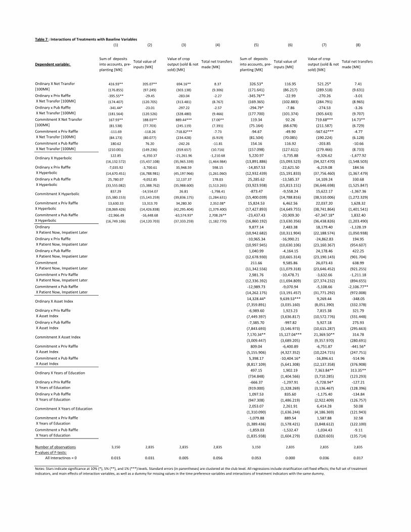
Table 7 : Interactions of Treatments with Baseline Variables
(1) (2) (3) (4) (5) (6) (7) (8)
Dependent variable:
Sum of deposits into accounts, pre-‐planting [MK]
Total value of inputs [MK]
Value of crop output (sold & not sold) [MK]
Total net transfers made [MK]
Sum of deposits into accounts, pre-‐planting [MK]
Total value of inputs [MK]
Value of crop output (sold & not sold) [MK]
Total net transfers made [MK]
416.93** 205.07** 694.16** 8.37 326.53* 116.95 521.25* 7.41(176.855) (97.249) (303.138) (9.306) (171.641) (86.217) (289.518) (9.631)-‐395.55** -‐29.45 -‐283.04 -‐2.27 -‐345.76** -‐22.99 -‐270.26 -‐3.01(174.407) (120.705) (313.481) (8.767) (169.365) (102.883) (284.791) (8.965)-‐341.44* -‐23.01 -‐297.22 -‐2.57 -‐294.79* -‐7.86 -‐274.53 -‐3.26(181.564) (120.526) (328.480) (9.466) (177.700) (101.374) (305.643) (9.707)167.93** 188.03** 889.44*** 17.00** 119.34 92.26 719.68*** 14.73**(81.538) (77.703) (245.119) (7.391) (75.164) (68.678) (211.587) (6.729)-‐111.69 -‐118.26 -‐718.82*** -‐7.73 -‐94.67 -‐49.90 -‐567.62*** -‐4.77(84.173) (80.077) (234.428) (6.919) (81.504) (70.085) (190.224) (6.128)180.62 76.20 -‐242.26 -‐11.81 154.16 116.92 -‐203.85 -‐10.66
(210.001) (149.236) (359.657) (10.716) (157.098) (127.611) (279.466) (8.733)122.85 -‐6,350.37 -‐21,261.96 -‐1,210.68 5,220.97 -‐3,735.88 -‐9,326.62 -‐1,677.92
(16,132.572) (15,437.108) (35,965.339) (1,464.984) (13,891.886) (15,093.523) (34,327.470) (1,548.503)-‐7,035.92 -‐3,700.61 35,948.59 598.15 -‐14,857.53 -‐22,621.50 -‐6,219.08 184.56
(14,670.451) (16,788.981) (45,197.966) (1,261.060) (12,932.439) (15,191.833) (37,756.460) (1,367.479)25,780.07 -‐9,052.85 12,137.37 178.03 25,285.62 -‐13,585.37 14,109.24 330.68
(33,555.082) (15,388.762) (35,988.600) (1,513.265) (33,923.938) (15,813.151) (36,646.698) (1,525.847)837.29 -‐14,554.07 26.81 -‐1,798.41 -‐873.47 -‐9,558.24 15,622.17 -‐1,367.36
(15,380.153) (15,143.259) (39,836.175) (1,284.631) (15,400.039) (14,788.816) (38,510.006) (1,272.329)13,630.33 13,313.70 34,280.30 2,352.08* 15,824.53 6,462.56 22,037.20 1,628.32
(18,069.426) (14,426.838) (42,295.404) (1,379.400) (17,427.893) (14,649.755) (38,741.864) (1,401.541)-‐22,966.49 -‐16,448.68 -‐63,574.93* 2,708.26** -‐23,437.43 -‐20,909.30 -‐67,347.18* 1,832.40(16,749.106) (14,120.703) (37,333.259) (1,182.770) (16,860.192) (13,630.356) (36,438.826) (1,203.490)
9,877.14 2,483.38 18,179.40 -‐1,128.19(10,942.682) (10,311.904) (22,188.574) (1,050.938)-‐10,965.34 -‐16,990.21 -‐24,862.83 194.95(10,997.945) (10,630.106) (23,160.367) (954.607)1,040.99 -‐4,164.15 24,178.46 422.25
(12,678.930) (10,665.314) (23,190.143) (901.704)211.66 9,585.86 26,073.43 638.99
(11,342.556) (11,079.318) (23,646.452) (921.255)2,981.76 -‐10,478.71 -‐3,632.66 -‐1,211.18
(12,336.392) (11,694.809) (27,374.232) (894.655)-‐12,989.73 -‐9,070.94 -‐5,108.66 -‐2,106.77**(14,262.175) (13,191.457) (31,771.292) (972.008)14,328.44* 9,639.53*** 9,269.44 -‐348.05(7,359.891) (3,035.160) (8,051.390) (332.378)-‐6,989.60 1,923.23 7,815.38 321.79(7,449.397) (3,636.817) (10,572.776) (331.448)-‐7,385.70 -‐997.82 5,927.18 275.93(7,843.693) (3,546.973) (10,615.287) (295.663)7,170.34** 15,127.04*** 21,369.50** 314.78(3,009.447) (3,689.205) (9,357.970) (280.691)809.04 -‐6,400.89 -‐6,751.87 -‐441.56*
(5,155.906) (4,327.352) (10,224.715) (247.751)5,398.17 -‐10,404.16* -‐16,896.61 -‐514.96
(8,817.109) (5,641.308) (12,137.358) (376.908)497.15 1,902.19 7,363.84** 313.35**
(734.848) (1,404.566) (3,710.285) (123.293)-‐666.37 -‐1,297.91 -‐5,728.94* -‐127.21(919.000) (1,328.269) (3,136.467) (128.396)1,097.53 835.60 -‐1,175.40 -‐134.84(947.308) (1,486.219) (2,922.409) (126.757)2,053.07 2,261.91 6,414.28 50.08
(1,310.090) (1,636.244) (4,186.369) (121.943)-‐1,079.88 889.54 1,587.88 32.58(1,389.436) (1,578.421) (3,848.612) (122.100)-‐1,859.03 -‐1,532.47 -‐1,034.43 -‐9.11(1,835.938) (1,604.279) (3,820.603) (135.714)
Number of observations 3,150 2,835 2,835 2,835 3,150 2,835 2,835 2,835P-‐values of F-‐tests:
All Interactinos = 0 0.015 0.031 0.005 0.056 0.053 0.000 0.036 0.017
Notes: Stars indicate significance at 10% (*), 5% (**), and 1% (***) levels. Standard errors (in parentheses) are clustered at the club level. All regressions include stratification cell fixed effects; the full set of treatment indicators, and main effects of interaction variables, as well as a dummy for missing values in the time preference variables and interactions of treatment indicators with the same dummy.
Ordinary X Patient Now, Impatient LaterOrdinary x Priv Raffle X Patient Now, Impatient LaterOrdinary x Pub Raffle X Patient Now, Impatient LaterCommitment X Patient Now, Impatient LaterCommitment x Priv Raffle X Patient Now, Impatient LaterCommitment x Pub Raffle X Patient Now, Impatient Later
Ordinary X Years of Education
Ordinary x Priv Raffle X Years of EducationOrdinary x Pub Raffle X Years of Education
Ordinary X Net Transfer[100MK]Ordinary x Priv Raffle X Net Transfer [100MK]Ordinary x Pub Raffle X Net Transfer [100MK]Commitment X Net Transfer[100MK]Commitment x Priv Raffle X Net Transfer [100MK]Commitment x Pub Raffle X Net Transfer [100MK]
Ordinary X Hyperbolic
Ordinary x Priv Raffle X HyperbolicOrdinary x Pub Raffle X Hyperbolic
Commitment X Hyperbolic
Commitment x Priv RaffleX HyperbolicCommitment x Pub RaffleX Hyperbolic
Commitment X Years of Education
Commitment x Priv Raffle X Years of EducationCommitment x Pub Raffle X Years of Education
Ordinary X Asset Index
Ordinary x Priv Raffle X Asset IndexOrdinary x Pub Raffle X Asset Index
Commitment X Asset Index
Commitment x Priv Raffle X Asset IndexCommitment x Pub Raffle X Asset Index
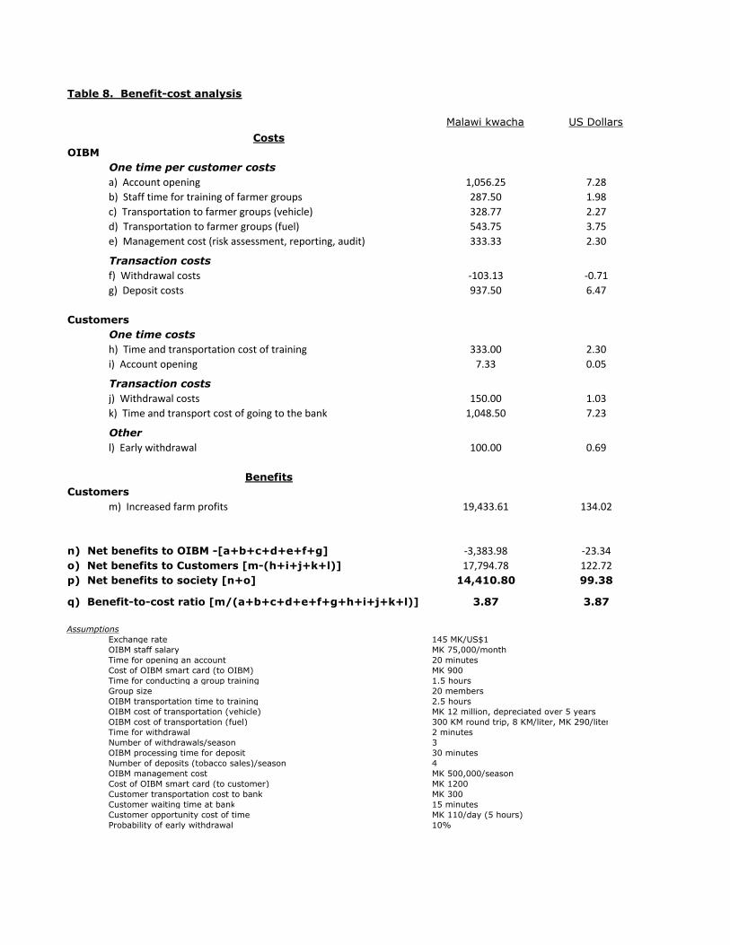
Table 8. Benefit-cost analysis
Malawi kwacha US Dollars
CostsOIBM
One time per customer costsa) Account opening 1,056.25 7.28
b) Staff time for training of farmer groups 287.50 1.98
c) Transportation to farmer groups (vehicle) 328.77 2.27
d) Transportation to farmer groups (fuel) 543.75 3.75
e) Management cost (risk assessment, reporting, audit) 333.33 2.30
Transaction costsf) Withdrawal costs 103.13 0.71
g) Deposit costs 937.50 6.47
CustomersOne time costsh) Time and transportation cost of training 333.00 2.30
i) Account opening 7.33 0.05
Transaction costsj) Withdrawal costs 150.00 1.03
k) Time and transport cost of going to the bank 1,048.50 7.23
Otherl) Early withdrawal 100.00 0.69
BenefitsCustomers
m) Increased farm profits 19,433.61 134.02
n) Net benefits to OIBM -[a+b+c+d+e+f+g] 3,383.98 23.34
o) Net benefits to Customers [m-(h+i+j+k+l)] 17,794.78 122.72
p) Net benefits to society [n+o] 14,410.80 99.38
q) Benefit-to-cost ratio [m/(a+b+c+d+e+f+g+h+i+j+k+l)] 3.87 3.87
AssumptionsExchange rate 145 MK/US$1OIBM staff salary MK 75,000/monthTime for opening an account 20 minutesCost of OIBM smart card (to OIBM) MK 900Time for conducting a group training 1.5 hoursGroup size 20 membersOIBM transportation time to training 2.5 hoursOIBM cost of transportation (vehicle) MK 12 million, depreciated over 5 yearsOIBM cost of transportation (fuel) 300 KM round trip, 8 KM/liter, MK 290/literTime for withdrawal 2 minutesNumber of withdrawals/season 3OIBM processing time for deposit 30 minutesNumber of deposits (tobacco sales)/season 4OIBM management cost MK 500,000/seasonCost of OIBM smart card (to customer) MK 1200Customer transportation cost to bank MK 300Customer waiting time at bank 15 minutesCustomer opportunity cost of time MK 110/day (5 hours)Probability of early withdrawal 10%
31
Appendix A: Account details and full text of training script
Savings account details In this experiment we offered farmers training and account opening assistance for two types
of accounts depending on the treatment status (control, ordinary savings or commitment savings). The �“ordinary�” account referred to in the main text is OIBM�’s Kasupe account. Kasupe accounts had an account opening of MK500, no monthly fee, three free withdrawals transactions via ATM per month, and a MK25 fee per ATM withdrawal thereafter (all withdrawals at the teller were free). The minimum balance for Kasupe accounts was MK1,000 and there was an account closing fee of MK1,000. Kasupe accounts paid an interest rate of 2.5% p.a. with interest accruing quarterly. Deposit transactions into Kasupe accounts were free.
Farmers were given the option to have their proceeds directly deposited into an existing account if they already had a savings account with OIBM. Another type of savings account not actively marketed in this experiment but part of OIBM�’s product portfolio was standard savings accounts with the following fee structure: an opening fee of MK500; a monthly fee of MK75; no withdrawal fees; minimum balance of MK1,000; a closing fee of MK1,000; an interest rate of 6.5% p.a. with quarterly accrual. This less common account type is included in the category �“ordinary�” accounts together with Kasupe accounts.
The �“commitment�” account referred to in the main text was an account newly developed for the project called �“SavePlan.�” SavePlan accounts paid the same interest rate as Kasupe accounts, but had no minimum balance requirement. SavePlan accounts also had no account opening or closing fees. . Deposit transactions into SavePlan accounts were free. The only withdrawals permitted for SavePlan accounts were transfers to ordinary (Kasupe or other) savings accounts, for which no fee was charged.
Scripts for savings training, account offers, and raffle training (Scripts were administered in club meeting immediately following administration of baseline
survey. Malawian research project staff played the roles of Persons 1 and 2.) Section 1: Savings Accounts (All Clubs) Person 1: Saving money in an individual bank account is a very smart way to protect your money and
improve your wellbeing. As you know, OIBM has Kasupe accounts that are easy and affordable to use. Person 2: But I already have a savings account with my club. What is better about this Kasupe account? First ask the group to list things that are good about the Kasupe account. When the group has come up with
several suggestions, move on to the next line: Person 1: The Kasupe account is yours alone. You don�’t share it with the rest of your club members. You are
the only one who can take money out of the account and the only one who knows how much money you have saved in the account.
Person 2: What are the details of the account? How much does it cost, and what is the interest? Person 1: MK 500 for smartcard, MK 500 for initial deposit, no monthly charge, MK 25 transaction charge
(ATM fee, withdrawal fee). Person 2: But I can just keep money at home. What are some of the benefits of saving my money in a Kasupe
account instead of at home?

32
Let the group make suggestions. After several things have been suggested, agree with the group and then
move on to the next line. Person 1: Money is safer in a bank account than at home. If you keep your money at home, it could be stolen
or lost in a fire. If you keep it at the bank, it is protected. Also, if you keep money at home, you may feel obligated to give money to your family or friends if they ask for it. If your money is in the bank, you can say that you don�’t have any money to give.
Person 2: That is interesting, but I think my money is safe at home. Ask the group: �“Do you think money is safe at home?�” Let the group come up with answers, then move on. Person 1: There are other reasons to keep money in the bank, too. Keeping money in a bank account can help
you save for the future. If you have money at home, it is easy to be tempted to spend it on food or drinks or household items. If you have money in the bank, you will think twice about taking it out to spend. Instead, you can leave it in the bank to save for important purchases like school fees or buying fertilizer or accumulating the deposit for a new loan. Also, you can be sure to put away money in case you have an emergency in the future, like someone gets sick and needs to go to the hospital.
Section 2: Saving for the future (All Clubs) Person 2: It would be good to save for the future, but I have many needs now. How can I afford to save? Person 1: It is important to make a plan for how to spend your money. One way to do this is to divide the
money you will have after selling your tobacco and paying your loans into two amounts. One amount is to use now, and the other amount is to use in the future. Then, you can commit to keeping the future amount safe, and not touching it now.
Person 2: How can I do that? Person 1: Think about how much money you will have after you sell your tobacco and repay your loan to
OIBM. Then, think about expenses you have immediately. Have the group list things they need to spend money on immediately. Get a list of 5-6 things, then move on. Person 2: Yes, I will have to pay someone who has done weeding for me. Also, I need to buy some soap and
other household goods. My children need new clothes, too. Person 1: Yes, these are the kinds of things you need to spend money on right away, when you get paid. But
now think of things you will need to spend money on in the future. What do you want to be absolutely sure you can afford?
Ask the group to list things they want to save for in the future. Make sure they are thinking of long-term things
or expenses that will happen in a few months. Get the group to list 5-6 things, then move on. Person 2: I can think of many things. I will need to pay school fees. Also, I want to make sure I can buy
fertilizer for my maize. And I want to have money for food next year during the hungry season. Person 1: These are important expenses. You should plan to protect some of your money so that it is
available for those expenses. You can do that by committing to locking it away until a date in the future, when you will need it. What is a date that makes sense? Choose a time that is close to when you will need the money for the reasons you just described, so that you aren�’t tempted to spend it on other things.
Ask the group: �“When do you think you want to access money you would save for the future?�” Let the group
discuss several dates. Make sure they consider purchasing inputs, and also food during the hunger season.

33
Person 2: Hmmm. November 1 is probably a good time. That will be in time for me to buy fertilizer and pay
my loan deposit. Person 1: Now that you have chosen a date, you have to decide how to divide your money between things you
will buy before that date, and the things you are saving for in the future. This is an important choice. You have to make sure that you have enough money for your immediate needs and things you will have to buy before the date you have chosen. You also have to estimate how much money you will need for the things you want to buy in the future. Start with money you need soon. Of the money you will have after you sell your tobacco and repay your loan, how much do you need to have available for spending before November 1, which is the date you have chosen?
Have the group suggest amounts of money they will spend on immediate expenses. Person 2: Well, I need to pay someone for ganyu. And I need to buy clothes, and some household items right
away. I will also need to spend some money after the harvest season on small things like soap. I will need to spend MK 25,000 between when I get money and November 1.
Person 1: Ok. How much do you want to make sure to have for the future, after that date you have chosen? Person 2: I will need MK 4,500 for fertilizer, and MK 3,000 for a deposit on a new loan. Also, I want to keep
MK 2,000 for food in the hungry season. That is MK 9,500 total. Person 1: So in total, your plan is to spend at least MK 25,000 now, and MK 9,500 in the future. That is MK
34,500. Do you think you will have at least that much profit after selling your tobacco and repaying your loan? Person 2: Yes, I think I will have about MK 40,000. Person 1: Good. If you earn that much, then the extra money can be available immediately. Then you can
commit to saving MK 9,500 for the future, and keep your other money available to spend sooner. You don�’t have to spend it all before your date of November 1, of course, but it will be available while you are committing to lock away MK 9,500 until then. You made three decisions: You decided how much money you needed immediately, you decided how much money to lock away for the future, and you decided when you needed to access that locked away money.
Person 2: Yes. Those weren�’t hard decisions. But let�’s demonstrate how it would work if I had chosen
different options. Section 3: Account Allocation Demonstration (All Clubs) In this section, the two enumerators will work together to do a demonstration with bottle caps. You will need
12 bottle caps for this demonstration. Draw two big circles in the dirt, and make sure everyone can see them. These circles represent money available for use immediately (point at one circle) and money committed to be
saved for the future (point at the other circle). These bottle caps represent money. Think of each cap as MK 1,000. So, the 12 caps I have here represent MK 12,000 that someone has after selling his crop and repaying his loan.
Now, if I need MK 3,000 now and commit to saving MK 5,000 for the future, then the first MK 3,000 I earn
goes in this circle, for use immediately (put 3 bottle caps in the immediate use circle). Then, the next MK 5,000 I earn gets locked away for the future (put 5 bottle caps in the future circle). Any extra money is available for use in the future, even though I don�’t have to spend it immediately it is not locked away (put the remaining 8 bottle caps in the immediate use circle).
(Collect all of the bottle caps). Think of this like a debt. I owe the ordinary account 3 bottle caps, and I owe
the commitment account 5 bottle caps. I must pay the ordinary account first, before I pay the commitment account. Suppose I get 10 bottle caps after I sell my tobacco and repay my loans. (Hold up 10 caps).

34
First, I put 3 for immediate use. (Put 3 caps in the immediate use circle.) Next, I lock 5 away for use in the future. (Put 5 caps in the future use circle.) Then, since I�’ve met the targets for immediate use and future use, I put all the other caps in the immediate use circle. (Put the remaining 2 caps in the immediate use circle.)
What if I only get 3 caps? (Have someone come up to demonstrate. Give the person 3 caps. See where he puts
them. All 3 should go in the immediate circle, and none in the future circle. If he gets this wrong, ask if anyone has a different idea. Explain if necessary.)
(Enumerator, if farmers don�’t understand the demonstration you just performed, please skip back to the start
of the demonstration and explain the bottle caps idea again.) What if I get 6 caps? (Have a volunteer come up and give him 6 caps. Correct answer: 3 in immediate, 3 in
future.) What if you get 12 caps? (Have another volunteer come up, etc. Correct answer: first put 3 in immediate,
then 5 in future, then 4 more in immediate. Total is 7 immediate, 5 in future.) Dividing the bottle caps between the two circles is just like the spending plan you made before. You decide
how much money you need to have available for immediate use. When you get money, it is first made available for immediate use, up to the goal you set. (Point at the immediate use circle). Then, you decide how much to save for the future. After making sure you have money for immediate use, you protect money for the future. (Point at the future use circle). Then, if there is money left after you meet both your immediate and future goals, that extra money remains available for use whenever you choose. (Point at the immediate use circle). This way, you can make a plan for how to divide your money between money you need now, and money you can commit to saving for the future, even when you don�’t know exactly how much you will earn.
Section 4: Offer of Kasupe (Ordinary) Accounts (All Clubs Except Group 0) Person 1: We have talked a lot about how to make a budget that gives you enough money for immediate needs
and commits you to saving money for the future. Also, we�’ve discussed why saving at the bank is useful. Person 2: Yes. I can make a plan about the amount of money I need for the short term, an amount I want to
be sure to save for the future, and a date in the future when I will want that money. But how am I to use the bank? Person 1: Usually, when you are paid for your tobacco, money is put into your group account. Then, the club
officers give you your share of the cash. You leave it in the group account if you want. Or, you can save it at the bank, but to do that, you have to take your cash to the bank and deposit it into your individual account.
Person 2: Yes. It is inconvenient to have to take the money back to the bank, and often, I am tempted to
spend the money as soon as I receive it. Person 1: This season, we are offering you a new option. You can sign up to have your money transferred
directly into your own Kasupe account. That means that when your bales of tobacco clear the auction floor, OIBM would automatically put the money you have earned after repaying your loan into your own Kasupe account.
Person 2: How would OIBM know which money was mine and which money belongs to others in my club? Person 1: You would have to agree that OIBM could get a copy of your seller sheet from Auction Holdings.
OIBM would use the information on the seller sheet to figure out how much money should go into your account. Person 2: So if I agree to this, what do I have to do? Person 1: The first thing to do is to open a Kasupe account, if you don�’t already have one. We can help with
filling out the forms. The next thing to do is to sign a form authorizing the direct deposit. You can do both of those things today.
35
Person 2: That�’s all I have to do? Person 1: Yes. It is very easy. If you open an account or already have one, and fill out the form for direct
deposit, then your money will be put into your individual account automatically when your tobacco is sold and your loan has been recovered.
Ask the group if there are any questions about how to sign up for direct deposit. Person 2: What if I decide I don�’t want to try this system and I would rather have my money go into the club
account? Person 1: You can still open a Kasupe account. Just don�’t fill out the [BLUE] form. Then, you will continue
to get your money from the club officers, who will withdraw it from the club account for you. But if you do choose to have the money sent directly to your individual account, then ALL of your money for tobacco this season will go to the individual account. You can�’t change your mind part way through the season.
Person 2: Ok. I think I want the direct deposit. If I sign up for that, how do I get my cash? Person 1: You can withdraw cash from the bank. You can either use your smartcard, or make the withdrawal
by talking to a teller. You can do this at the branch or kiosk, or when the mobile bank comes to town. The closest place to make a withdrawal is ______________.
Person 2: So I can take money out whenever I want? Person 1: Yes, you can, but you should remember the commitment you thought about to save money for a
date in the future. Section 5: Offer of SavePlan (Commitment) Accounts (Commitment Clubs Only) Person 2: Is there a way that OIBM can help me keep that commitment? Person 1: Yes. You can open a special �“SavePlan�” account in addition to your Kasupe account. Person 2: How would that work? Person 1: Opening a SavePlan just tells the bank to follow the plan you made before. You will fill out a form
with the three decisions you made earlier: how much money you need to have available for immediate use, the amount of money you want to lock away for the future, and the date you want that money released.
Person 2: That is easy. It�’s just writing down decisions I�’ve already thought about. What happens after I fill
out the form? Person 1: Once you fill out the form, OIBM will use it to put the money you are saving for the future in a
special, individual, commitment account. You won�’t be able to take money out of that account until the date you have chosen, and you can�’t change your mind about the date or the amount of money.
Person 2: Do I earn interest on money in this special account? Person 1: Yes. You earn the same interest on money in the commitment account as in the ordinary Kasupe
account. The only difference is that the money in the commitment account is locked away until the date you have chosen.
Person 2: What if I earn more or less money than I thought I would have? Person 1: It works just like the bottle caps. After the loan is recovered, money first goes into your ordinary
Kasupe account, up to the amount you said you needed to have available immediately. Then, money goes to the

36
SavePlan to be locked away for the future. When you have reached your target for saving for the future, extra money earned after that amount goes back to the ordinary Kasupe account.
Person 2: So if I don�’t earn as much as I thought, I will still have money available immediately? Person 1: Yes. Money goes to the Kasupe account first, and you can withdraw from that whenever you want.
It only goes to the special commitment account when you have reached your target for immediate spending. Person 2: So this form just tells the bank to stick to the commitment I made to myself about how much to save
for the future, and when I can use that money. Person 1: That�’s right. You can choose any amount and date you want, and OIBM will hold it for you so that
you stick to the plan. We can help you fill out the form if you would like to use this special account in addition to the regular Kasupe account.
Section 6: Raffle (All Raffle Clubs) As an extra incentive to save money, there will be a raffle draw where some farmers in this project may have a
chance to win a prize. You have to save to have a chance to win, and the more you save, the better your chance to win. There will be two prizes in each district. The first prize will be a new bicycle, and the second prize will be a 50 kg bag of D-compound.
The raffle tickets will be based on the amount of money you save in your bank account. The prizes will be
awarded in November. The raffle tickets will be given out at two times before then. The first time will be in August when we will come back and give you tickets based on the money you have saved between July 1 and August 1. OIBM will calculate the average balance in your savings account for those 30 days and the number of tickets you will get will be based on this amount. The second time we hand out tickets will be in October. OIBM will calculate your average balance from September 1 to October 1, and give you additional tickets based on that balance. Each person will get individual tickets based on their account balance. The prize is for individuals and not for the club.
You can increase your chance of winning by saving more money and saving it for a longer time. You will get
one ticket for every MK 1000 in your average balance. If you put MK 10000 in your account by July 1 and keep it there until at least August 1, then you will get 10 tickets. If you don�’t have any money in your account from July 1 to July 14, and then put MK 10000 into your account on July 15 and keep it there until at least August 1, you will only get five tickets. If anyone here has two accounts with OIBM, we will add up the balance in both accounts. Money saved with other banks will not count for the raffle, though.
Section 7A: Public Raffle (Public Raffle Clubs Only) We will hand out the raffle tickets in August and October during group meetings like the one we are having
today. We will give out the tickets in front of others, so your friends will know how many tickets you are getting. I will demonstrate how tickets will be handed out. I am going to hand you a piece of paper with a number on
it. Pretend that is your average account balance from July 1 to August 1. No one but you and OIBM knows this number, so don�’t tell anyone!
(Distribute the papers with fake account balances to 5 volunteers) Now, I will give you the number of raffle tickets you get for that balance. Come up one at a time and show me
your piece of paper, so I can give you your tickets. (Have the farmers come up one at a time. Look at the paper and hand out tickets. Make sure to say out loud
for every farmer how many tickets he gets. Make sure that the other farmers are paying attention to this.)

37
When we hand out tickets in August and October, it will work the same way. You will each be called up one at a time to receive tickets based on the amount you have saved, and your club will see how many tickets you receive.
Section 7B: Private Raffle (Private Raffle Clubs Only) We will hand out the raffle tickets in August and October during group meetings like the one we are having
today. We will give out the tickets one at a time, so no one will know how many tickets you are getting. I will demonstrate how tickets will be handed out. I am going to hand you a piece of paper with a number on
it. Pretend that is your average account balance from July 1 to August 1. No one but you and OIBM knows this number, so don�’t tell anyone!
(Distribute the papers with fake account balances to 5 volunteers) Now, I will give you the number of raffle tickets you get for that balance. Come up one at a time and show me
your piece of paper, so I can give you your tickets. (Have the farmers come up one at a time. Look at the paper and hand out tickets. Make sure no one sees how
many tickets you hand to each person.) When we hand out tickets in August and October, it will work the same way. You will each be called up one
at a time to receive tickets based on the amount you have saved, and no one will know how many tickets you have received.

38
Appendix B: Variable definitions Data used in this paper come from two surveys as well as from administrative records of our
partner financial institution (OIBM). We conducted a baseline survey from March to April 2009 and an endline survey from July to September 2010.
All variables that are created from survey data are top coded at the 99th percentile for variables with a positive range and bottom and top coded at the 1st and 99th percentile respectively for variables with a range that spans both negative and positive values. All figures in money terms are in Malawi Kwacha (MK).
Baseline characteristics (from baseline survey): Number of members per club is the number of listed club members per information provided
by the buyer companies (Alliance One and Limbe Leaf). Not all club members were interviewed. Female equals 1 for female respondents and 0 for male respondents. Married equals 1 for married respondents and 0 for respondents who are single, widowed, or
divorced. Age is respondent�’s age in years. Years of education is the respondent�’s years of completed schooling. Household size is the number of people counted as members of the respondent�’s household
at the time of the baseline survey. Asset index is an index based on the first principal component of the number of items owned
of 14 common non-financial, non-livestock assets and indicators of presence of 4 major types of housing characteristics (iron sheet roof, glass windows, concrete floor, electricity connection).
Livestock index is an index based on the first principal component of the number of animals owned of 7 common types of livestock.
Land under cultivation is the total of area of land under cultivation, measured in acres, for the late-2008 planting season.
Proceeds from crop sales is the sum of sales from maize and tobacco in the 2008 harvest. Cash spent on inputs is the total amount of cash spent �– excluding the value of input
packages that are part of a loan -- on seeds, fertilizer, pesticides, and hired labor for the 2008-2009 planting season
Has bank account is 1 if a household member has an account with a formal financial institution, and 0 if not.
Savings in accounts and cash is the sum of current savings with formal institutions and in cash at home.
Hyperbolic is 1 if the respondent exhibited strictly more patience in one month, hypothetical monetary trade-offs set 12 months in the future than in the same trade-offs set in the present, and 0 otherwise. See section 5 above for more details.
Patient now, impatient later is 1 if the respondent exhibited strictly less patience in one month, hypothetical monetary trade-offs set 12 months in the future than in the same trade-offs set in the presence and 0 otherwise.
Net transfers made in past 12m is the total of transfers made to the social network minus the sum of transfers received from the social network, summed across six categories (social events, health shocks, education of children, agricultural inputs, hired labor and �‘other�’).
Missing value for formal savings and cash is 1 if the variable �“Savings in accounts and cash�” is missing and 0 if it has valid values.

39
Missing value for time preferences is 1 if the respondent has missing values for the time preferences variables (�“Hyperbolic�” and �“Patient now,impatient later�”) is missing, and 0 if these variables have valid values.
Transactions with Partner Institution (from internal records of OIBM): Any transfer via direct deposit is 1 if the respondent receives any deposit from his or her
tobacco club�’s account to his or her individual savings account, and 0 if not. Deposits into ordinary accounts, pre-planting is the sum of (positive) transactions into the
respondent�’s OIBM ordinary savings accounts during the period of March to October 2009. Deposits into commitment accounts, pre-planting is the sum of (positive) transactions into
the respondent�’s OIBM commitment savings accounts during the period of March to October 2009.
Deposits into other accounts, pre-planting is the sum of (positive) transactions into the respondent�’s OIBM non-ordinary, non-commitment savings accounts during the period of March to October 2009.
Sum of deposits into accounts, pre-planting is the sum of (positive) transactions into the respondent�’s OIBM accounts (sum across all accounts) during the period of March to October 2009.
Sum of withdrawals from accounts, pre-planting is the sum of (negative) transactions out of the respondent�’s OIBM accounts (sum across all accounts) during the period of March to October 2009.
Net of all transactions, pre-planting is the difference between the sum of all deposits and withdrawals in the respondent�’s OIBM accounts during the period of March to October 2009.
Net of all transactions, planting is the difference between the sum of all deposits and withdrawals in the respondent�’s OIBM accounts during the period of November 2009 to April 2010.
Agricultural outcomes, household expenditure, and other variables, from endline survey (all
planting and harvest variables refer to the 2009-2010 planting season): Land under cultivation is the total area of land under cultivation, measured in acres. Total value of inputs is the sum of cash spent on agricultural inputs plus the value of inputs
included in-kind in loan packages for the 2009-2010 planting season. Input categories include seeds, pesticides, fertilizer, hired labor, transport and firewood (for curing tobacco).
Proceeds from crop sales is the revenue from crop sales across all crops sold. Value of crop not sold is kilograms of crops not sold multiplied by the price/kilogram,
summed across all crops. Price/kilogram for each crop is obtained by calculating crop-specific revenue/kilogram for each observation in the sample and then taking the sample average.
Value of crop output (sold & not sold) is the sum of �“Proceeds from crop sales�” and �“Value of crop not sold�” defined above.
Farm profit (output - input) is the difference between �“Value of crop output�” and �“Total value of inputs�” defined above.
Total expenditure in last 30 days is the sum of three categories household expenditures (food, non-food household items and transport) over the last 30 days prior to the endline survey.
Household size is the number of people counted as members of the respondent�’s household at the time of the endline survey.

40
Total transfers made is the total of transfers made to the social network over the 12 months prior to the endline interview, summed across six categories (social events, health shocks, education of children, agricultural inputs, hired labor and �‘other�’).
Total transfers received is the total of transfers received from the social network over the 12 months prior to the endline interview, summed across six categories (social events, health shocks, education of children, agricultural inputs, hired labor and �‘other�’).
Total net transfers made is the difference between �“Total transfers made�” and �“Total transfers received�” defined above.
Transfers made, biggest gift bf. Oct09 is the same variable as �“Transfers made�” above with the sum of transfers restricted to categories in which the biggest gift was made before or in October 2009.
Transfers received, biggest gift bf. Oct09 is the same variable as �“Transfers received�” above with the sum of transfers restricted to categories in which the biggest gift was made before or in October 2009.
Total net transfers made, biggest gift bf. Oct09 (MK) is the difference between �“Transfers made, biggest gift bf. Oct09�” and �“Transfers received, biggest gift bf. Oct09�” as defined above.
Has fixed deposit account is 1 if the respondent has a fixed deposit account with any bank, and 0 if not.
Not interviewed in endline is 1 if the respondent was not interviewed and is 0 if the respondent was interviewed during the endline survey of July to September 2010.

Appendix Table 1: Attrition from Baseline to Endline Survey
(A) (B)Including Baseline Controls No Baseline controls
Dependent variable: Not interviewed during endline
surveyNot interviewed during endline
survey
Ordinary Account -‐0.00 0.00(0.03) (0.03)
Ordinary x Private Raffle -‐0.03 -‐0.04(0.02) (0.02)
Ordinary x Public Raffle 0.01 0.01(0.03) (0.03)
Commitment Account 0.00 0.01(0.02) (0.03)
Commitment x Private Raffle -‐0.01 -‐0.02(0.02) (0.02)
Commitment x Public Raffle -‐0.01 -‐0.00(0.02) (0.02)
Mean Dep Var in Control 0.099 0.099Number of observations 3,150 3,150
P-‐values of F-‐tests:Ordinary, No Raffle = Commitment, No Raffle 0.802 0.790Ordinary, Private Raffle = 0 0.085 0.096Ordinary, Public Raffle = 0 0.680 0.519Commit., Private Raffle = 0 0.764 0.711Commit., Public Raffle = 0 0.775 0.883Private Raffle = 0, Ordinary or Commitment (jointly) 0.923 0.774Public Raffle = 0, Ordinary or Commitment (jointly) 0.079 0.049
Notes: Stars indicate significance at 10% (*), 5% (**), and 1% (***) levels. Standard errors are clustered at the club level. Regressions include stratification cell fixed effects.

Appendix Table 2: Impact of Treatments on Deposits and Withdrawals
Regressions with stratification cell fixed effects but without additional baseline controls
(1) (2) (3) (4) (5) (6) (7) (8)
Dependent variable: Any Transfer via Direct Deposit
Deposits into ordinary accounts, pre-‐planting [MK]
Deposits into commitment accounts, pre-‐planting [MK]
Deposits into other accounts, pre-‐planting [MK]
Sum of deposits into accounts, pre-‐
planting [MK]
Sum of withdrawals from accounts, pre-‐
planting [MK]
Net of all transactions, pre-‐planting [MK]
Net of all transactions, planting [MK]
Ordinary Account 0.17*** 22,927.66*** -‐77.07 329.61 23,180.20*** -‐22,507.50*** 672.70 -‐915.71(0.05) (7,744.01) (229.74) (263.08) (7,845.12) (7,525.24) (1,033.92) (654.82)
Ordinary x Private Raffle 0.00 -‐13,265.82* -‐26.93 -‐502.45** -‐13,795.20* 14,103.27* 308.07 -‐49.17(0.05) (7,956.91) (248.51) (249.12) (8,051.13) (7,732.94) (1,099.16) (723.69)
Ordinary x Public Raffle 0.04 -‐553.43 51.71 -‐528.79** -‐1,030.51 53.44 -‐977.07 320.19(0.06) (10,138.38) (231.44) (243.48) (10,207.28) (10,079.24) (1,445.83) (731.34)
Commitment Account 0.22*** 21,061.32*** 1,981.98** 411.24 23,454.54*** -‐22,350.21*** 1,104.33 -‐1,366.52***(0.05) (6,544.53) (792.99) (351.68) (7,191.44) (7,097.81) (674.72) (507.63)
Commitment x Private Raffle 0.03 -‐3,317.70 -‐660.97 -‐139.70 -‐4,118.37 4,295.93 177.56 -‐152.98(0.06) (7,265.29) (907.34) (384.74) (7,950.51) (7,664.60) (966.01) (686.33)
Commitment x Public Raffle -‐0.06 -‐5,582.05 -‐829.90 -‐222.91 -‐6,634.86 7,052.44 417.58 -‐120.62(0.05) (7,960.91) (856.78) (365.10) (8,498.98) (8,282.86) (941.84) (608.45)
Mean Dep Var in Control 0.000 3107.045 0.000 174.087 3281.132 -‐3256.440 24.692 -‐157.774Number of observations 3,150 3,150 3,150 3,150 3,150 3,150 3,150 3,150
P-‐values of F-‐tests:Ordinary, No Raffle = Commitment, No Raffle 0.361 0.844 0.010 0.829 0.978 0.987 0.721 0.564Ordinary, Private Raffle = 0 0.001 0.033 0.637 0.272 0.044 0.067 0.024 0.018Ordinary, Public Raffle = 0 0.000 0.006 0.902 0.221 0.007 0.007 0.778 0.170Commit., Private Raffle = 0 0.000 0.001 0.006 0.322 0.001 0.001 0.092 0.005Commit., Public Raffle = 0 0.002 0.013 0.003 0.384 0.008 0.012 0.043 0.002Private Raffle = 0, Ordinary or Commitment (jointly) 0.250 0.781 0.624 0.827 0.737 0.696 0.905 0.971Public Raffle = 0, Ordinary or Commitment (jointly) 0.741 0.121 0.931 0.094 0.115 0.082 0.484 0.753
Notes: Stars indicate significance at 10% (*), 5% (**), and 1% (***) levels. Standard errors are clustered at the club level. USD 1 is ca. MK 145. All regressions include stratification cell fixed effects. F-‐tests: "Ordinary, No Raffle = Commitment, No Raffle" tests the equality of means in ordinary and commitment treatment groups each without additional raffle treatments; "Ordinary, Private Raffle = 0" tests if the sum of the coefficient on "Ordinary" and the coefficient on "Ordinary x Private Raffle" is different from zero; "Ordinary, Public Raffle", "Commitment, Private Raffle"; "Commitment, Public Raffle" tests the same sums of the different combinations of savings and raflle treatments; "Private Raffle = 0, Ordinary or Commitment (jointly)" tests whether the coefficient on the interaction of "Ordinary" and "Commitment" with "Private Raffle" are jointly different from zero; "Public Raffle = 0, Ordinary or Commitment (jointly)" peforms the same test but for the public raffle treatment condition.

Apendix Table 3: Impact of Treatments on Agricultural Outcomes and Household ExpenditureRegressions with stratification cell fixed effects but without additional baseline controls
(1) (2) (3) (4) (5) (6) (7)
Dependent variable: Land under cultivation
[acres]Total value of inputs
[MK]Proceeds from crop
sales [MK]Value of crop not sold
[MK]Value of crop output (sold & not sold) [MK]
Farmprofit (output-‐intput) [MK]
Total expenditure in last 30 days [MK]
Ordinary Account 0.11 10,792.53 14,450.53 142.22 14,706.67 6,739.15 831.83(0.22) (6,894.72) (12,828.80) (4,644.40) (15,541.74) (11,485.38) (955.61)
Ordinary x Private Raffle 0.25 -‐5,220.82 3,189.04 6,752.10 11,588.99 15,320.29 398.97(0.24) (7,495.04) (14,472.71) (4,697.05) (17,592.31) (12,898.56) (1,042.70)
Ordinary x Public Raffle 0.34 -‐932.42 10,603.13 6,135.39 17,831.64 17,189.02 923.13(0.23) (7,434.50) (14,246.94) (4,754.53) (16,935.35) (12,632.95) (958.83)
Commitment Account 0.46** 17,675.88** 27,933.83** 10,597.32* 40,811.44** 24,737.45* 2,260.27**(0.23) (7,449.82) (13,594.54) (5,873.96) (17,798.20) (13,528.35) (1,006.46)
Commitment x Private Raffle -‐0.07 -‐6,235.68 11,122.75 -‐9,391.86* -‐1,267.30 748.99 -‐378.69(0.23) (8,578.81) (16,491.84) (5,575.67) (19,799.98) (14,856.10) (1,038.19)
Commitment x Public Raffle -‐0.36 -‐12,837.01 -‐11,723.54 -‐7,791.88 -‐21,791.03 -‐8,328.11 -‐1,400.41(0.23) (8,014.85) (15,763.21) (5,740.00) (19,916.19) (15,049.14) (1,145.76)
Mean Dep Var in Control 4.275 59754.081 95196.514 55058.099 152408.056 92306.643 10678.419Number of observations 2,835 2,835 2,835 2,835 2,835 2,835 2,835
P-‐values of F-‐tests:Ordinary, No Raffle = Commitment, No Raffle 0.145 0.435 0.379 0.065 0.174 0.191 0.210Ordinary, Private Raffle = 0 0.123 0.339 0.166 0.150 0.101 0.079 0.172Ordinary, Public Raffle = 0 0.038 0.094 0.046 0.195 0.035 0.051 0.031Commit., Private Raffle = 0 0.075 0.075 0.007 0.788 0.017 0.053 0.030Commit., Public Raffle = 0 0.629 0.409 0.236 0.549 0.256 0.217 0.396Private Raffle = 0, Ordinary or Commitment (jointly) 0.250 0.258 0.369 0.237 0.438 0.791 0.449Public Raffle = 0, Ordinary or Commitment (jointly) 0.304 0.729 0.747 0.284 0.567 0.316 0.608
0.121
0.208
P-‐value of F-‐test of Ordinary= 0 across regressions of columns 1, 2, 5, 7: P-‐value of F-‐test of Ordinary=Commitment across regressions of columns 1, 2, 5, 7:
Notes: Stars indicate significance at 10% (*), 5% (**), and 1% (***) levels. Standard errors are clustered at the club level. USD 1 is ca. MK 145. All regressions include stratification cell fixed effects. F-‐tests: "Ordinary, No Raffle = Commitment, No Raffle" tests the equality of means in ordinary and commitment treatment groups each without additional raffle treatments; "Ordinary, Private Raffle = 0" tests if the sum of the coefficient on "Ordinary" and the coefficient on "Ordinary x Private Raffle" is different from zero; "Ordinary, Public Raffle", "Commitment, Private Raffle"; "Commitment, Public Raffle" tests the same sums of the different combinations of savings and raflle treatments; "Private Raffle = 0, Ordinary or Commitment (jointly)" tests whether the coefficient on the interaction of "Ordinary" and "Commitment" with "Private Raffle" are jointly different from zero; "Public Raffle = 0, Ordinary or Commitment (jointly)" peforms the same test but for the public raffle treatment condition.

Appendix Table 4: Impact of treatments on household size, transfers and fixed deposit
Regressions with stratification cell fixed effects but without additional baseline controls
(1) (2) (3) (4) (5) (6) (7) (8)
Dependent variable: Household sizeTotal transfers made (MK)
Total transfers received (MK)
Total net transfers made (MK)
Transf. made, biggest gift bf. Oct09 [MK]
Transf. received, biggest gif bf. Oct09 [MK]
Net transf. made, biggest gift bf. Oct09 [MK]
Has fixed deposit account
Ordinary Account 0.05 489.21 -‐206.04 640.60 23.64 -‐73.97 114.09 0.03**(0.11) (351.97) (322.25) (436.32) (88.18) (124.25) (139.92) (0.02)
Ordinary x Private Raffle 0.13 -‐556.78* -‐45.69 -‐444.96 61.93 -‐54.88 132.99 -‐0.03**(0.11) (333.92) (310.05) (442.31) (86.25) (126.51) (120.59) (0.02)
Ordinary x Public Raffle 0.16 -‐511.63 -‐201.35 -‐297.29 123.71 -‐97.25 205.42* -‐0.01(0.11) (372.17) (297.76) (401.69) (99.23) (113.73) (120.25) (0.02)
Commitment Account 0.06 275.31 -‐490.82* 722.28* 79.42 -‐272.34*** 358.63*** 0.06***(0.11) (330.32) (290.31) (405.30) (83.72) (104.66) (128.15) (0.02)
Commitment x Private Raffle 0.13 97.26 5.66 121.57 14.51 54.36 -‐48.79 -‐0.02(0.12) (380.59) (251.88) (403.44) (94.88) (97.73) (120.26) (0.03)
Commitment x Public Raffle 0.08 -‐21.21 517.82** -‐593.00 44.18 83.14 -‐35.75 -‐0.01(0.11) (336.37) (257.25) (399.41) (101.46) (100.80) (144.22) (0.03)
Mean Dep Var in Control 5.72 2871.70 2492.13 417.89 358.53 641.98 -‐297.32 0.04Number of observations 2,835 2,835 2,835 2,835 2,835 2,835 2,835 2,835
P-‐values of F-‐tests:Ordinary, No Raffle = Commitment, No Raffle 0.951 0.553 0.299 0.847 0.525 0.064 0.050 0.249Ordinary, Private Raffle = 0 0.115 0.820 0.423 0.643 0.291 0.297 0.045 0.972Ordinary, Public Raffle = 0 0.051 0.948 0.185 0.373 0.123 0.127 0.009 0.276Commit., Private Raffle = 0 0.114 0.325 0.104 0.053 0.312 0.064 0.022 0.018Commit., Public Raffle = 0 0.231 0.444 0.929 0.753 0.219 0.115 0.038 0.011Private Raffle = 0, Ordinary or Commitment (jointly) 0.547 0.951 0.074 0.187 0.909 0.684 0.916 0.685Public Raffle = 0, Ordinary or Commitment (jointly) 0.295 0.223 0.771 0.592 0.460 0.691 0.233 0.097
Notes: Stars indicate significance at 10% (*), 5% (**), and 1% (***) levels. Standard errors are clustered at the club level. USD 1 is ca. MK 145. All regressions include stratification cell fixed effects. F-‐tests: "Ordinary, No Raffle = Commitment, No Raffle" tests the equality of means in ordinary and commitment treatment groups each without additional raffle treatments; "Ordinary, Private Raffle = 0" tests if the sum of the coefficient on "Ordinary" and the coefficient on "Ordinary x Private Raffle" is different from zero; "Ordinary, Public Raffle", "Commitment, Private Raffle"; "Commitment, Public Raffle" tests the same sums of the different combinations of savings and raflle treatments; "Private Raffle = 0, Ordinary or Commitment (jointly)" tests whether the coefficient on the interaction of "Ordinary" and "Commitment" with "Private Raffle" are jointly different from zero; "Public Raffle = 0, Ordinary or Commitment (jointly)" peforms the same test but for the public raffle treatment condition.


