
Combinatorial Algorithms
Set Cover Problem
Set Cover
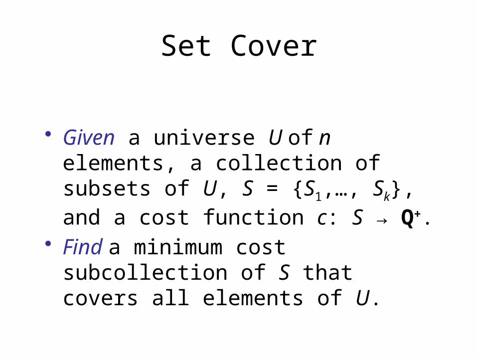
• Given a universe U of n elements, a collection of subsets of U, S = {S1,…, Sk}, and a cost function c: S → Q+.
• Find a minimum cost subcollection of S that covers all elements of U.

Greedy strategy
• Among the first strategies one tries when designing an algorithm for an optimization problem is some form of the greedy strategy.
• Greedy algorithms work by making a sequence of decisions; each decision is made to optimize that particular decision, even though this sequence of locally optimal decisions might not lead to a globally optimal solution.
• The advantage of greedy algorithms is that they are typically very easy to implement, and hence greedy algorithm are a commonly used heuristics, even when they have no performance guarantee.

The greedy algorithm
• Let C be the set of elements already covered at the beginning of an iteration. During this iteration, define the cost-effectiveness of a set Si to be the average cost at which it covers new elements? i.e., αi = c(Si)/|Si – C|.
• Define the price of an element to the average cost at which it is covered.
• Equivalently, when a set Si is picked, we can think of its cost being distributed equally among the new elements covered, to set their prices.

Chvatal’s Algorithm
0) Input (U, S, c: S → Q+)1) C , Sol 2) While C U do: Find Si S – Sol such that αi=c(Si)/|Si – C| is minimal. Sol Sol {Si} C С Si (Si is most cost-effective) Set price(e) = αi for all e Si – C3) Output (Sol)

Analysis of Chvatal’s Algorithm
• Number the elements of U in the order, in which were covered by the algorithm, resolving ties arbitrarily.
• Let e1,…,en be this numbering.
• Lemma 2.1
For each k {1,…,n}, price(ek) OPT/(n–k+1).

Proof of Lemma 2.1
ei,…,ek,…,en
e1,…,ei –1
OPT OPT OPTOPT
CS – C
In any iteration, the leftover sets of the optimal solution can cover theremaining elements at a cost of at most OPT.

Proof of Lemma 2.1
ei,…,ek,…,en
OPT OPT OPT
The total cost-effectivenessis at most OPT/(n – i + 1) OPT/(n – k + 1)
There must be one subset Sj S – C with αj OPT/(n – k + 1).
price(ek) OPT/(n–k+1).
n
n
n
n
n
n
b
a
bb
aa
b
a
ba
ba
1
1
2
2
1
1

Performance of the Chvatal Algorithm
Theorem 2.2 Chvatal’s Algorithm is an Hn factor approximation
algorithm for the minimum set cover problem, where Hn=1+1/2+1/3+…+1/n.
Proof.
OPTn
epriceScn
kk
CSi
i
121
11

Tight example
●●● 1+ ε
1/n 1/(n–1) 1/(n–2) 1/2 1
11
Vertex cover
• Given an undirected graph G = (V, E), and a cost function on vertices c: V → Q+.
• Find a minimum cost vertex cover.

Layering
• We introduce a technique of layering.• The idea in layering is to decompose the given
weight function on vertices into convenient functions, called degree-weighted, on a nested sequence of subgraphs G. For degree-weighted functions, we will show that we will be within twice the optimal even if we pick all vertices in the cover.

Degree-weighted function
• Let w: V → Q+ be the function assigning weights to the vertices of the given graph G = (V,E).
• We will say that a function assigning vertex weight is degree-weighted, if there is a constant с > 0, such that the weight of each vertex vV is с deg(v).
Lower Bound
• Lemma 2.3
Let w: V → Q+ be a degree-weighted function. Then w(V) 2 OPT.

Proof
• Let c be the constant such that w(c) = с deg(v), and let U be an optimal vertex cover in G. Since U covers all the edges,
.deg EvUv
• Therefore, w(U) ≥ c|E|. Now, since
.2 ,2deg EcVwEvVv

Largest degree-weighted function
• Let w: V → Q+ be an arbitrary function. • Let us define the largest degree-weighted function
in w as follows: – Remove all degree zero vertices from the graph, and over
the remaining vertices, compute c= min{w(v)/deg(v)}. – Then t(v) = c deg(v) is the desired function.
• Define w′(v) = w(v) – t(v) to be the residual weight function.

The Layer Algorithm
0) Input (G = (V, E), w: V → Q+)1) Sol , i 0, w′(v) w(v), V0 V – D0 (D0 ={v V |deg(v)=0}) 2) While Vi do: w′(v) w′(v) – ti(v) Sol Sol Wi (Wi ={v Vi |w′(v)=0}) Vi+1 Vi – Wi
i i+1 Vi Vi – Di (Di ={v Gi |deg(v)=0})3) Output (Sol)

Example
6 2
4
1
6
4
4
t(v) = 1 deg(v)

Example
3 1
0
0
2
1
2
Sol

Example
3 1
2
1
2
Sol
t(v) = (2/3) deg(v)

Example
5/3
0
1/3
2/3
Sol

Example
5/3
1/3
2/3
Sol
t(v) = (2/3) deg(v)

Example
Sol 4
164
15
6 2
4
1
6
4
4

Approximation ratio of the Layer Algorithm
Theorem 2.4 The Layer Algorithm achieves an
approximation guarantee of factor 2 for the vertex cover problem assuming arbitrary vertex weights.

Scheme of the Algorithm
Dk
Wk-1 Dk-1
W1 D1
W0 D0
●●●
Gk
Gk-1
G1
G0 =G
Sol
C*∩Gi is a vertex cover for Gi
Let t0,…,tk1 be the degree-weighted functions.

Proof of Theorem 2.4 (1)
• We need to show that set Sol is a vertex cover for G and w(Sol) ≤ 2 OPT.
• Assume, for contradiction, that Sol is not a vertex cover for G. Then there must be an edge (u,v) with uDi and vDj, for some i, j. Assume i ≤ j. Therefore, (u,v) is present in Gi, contradicting the fact that u is a degree zero vertex.

Proof of Theorem 2.4 (2)
• Let C* be an optimal vertex cover. • Consider a vertex v Sol. If v Wj, its weight can be
decomposed as
• Consider a vertex v V Sol. If v Dj, its weight can be decomposed as
.
ji
i vtvw
.
ji
i vtvw

Proof of Theorem 2.4 (3)
• C*∩Gi is a vertex cover for Gi.
• Lemma 2.3 ti(Sol∩Gi) ≤ 2 ti(C*∩Gi).
• By the decomposition of weights, we get
*).(2*2)(1
0
1
0
CwGCtGSoltSolwk
tii
k
tii

Tight example
1w
1w
1w
1w
1w
1w
1w
1w

Shortest Superstring
• Given a finite alphabet Σ, and a set of n strings S = {s1,…,sn} Σ+.
• Find a shortest string s that contains each si as a superstring.
• Without lost of generality, we may assume that no string si is a substring of another string sj, i j.

Shortest Superstring as Set Cover
sisj
k > 0
πijk
M ={πijk | πijk is a valid choice of i, j, k}
πM : set(π)={sS | s is a substring of π}
Ucover SstringScover {set(πijk) | πijk is a valid choice of i, j, k}
c(set(π)) = | π |

Lower bound
• Lemma 2.5
OPTstring OPTcover 2 OPTstring
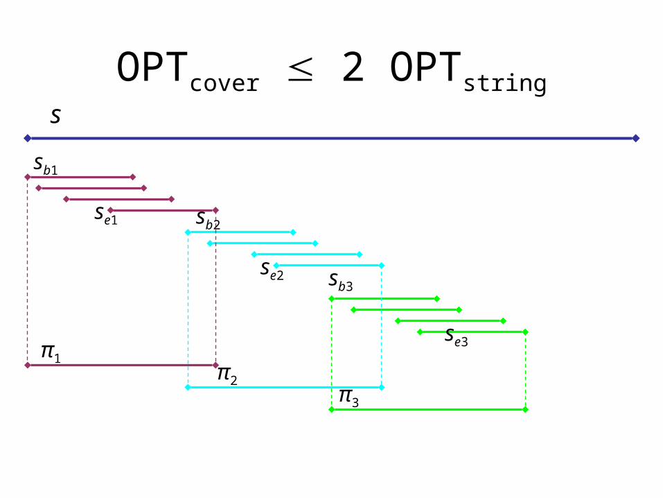
OPTcover 2 OPTstrings
sb1
se1 sb2
se2 sb3
se3π1π2
π3

Li’s Algorithm
1) Use the greedy set cover algorithm to find a cover for the instance S.
2) Let set(π1),…, set(πk) be the sets picked by this cover. 3) Concatenate the strings π1,…,πk in any order. 4) Output the resulting string, say s.

Approximation ratio of
Theorem 2.6 Li’s algorithm is a 2Hn factor algorithm for
the shortest superstring problem, where n is the number of strings in the given instance.

Exercises The bin packing problem with bounded number of
items per a bin.• Given n items and their sizes a1,…,an (0,1].
• Find a packing in unit-sized bins that minimizes the number of bin used under condition that each bin contains at most five items.
1. Reduce the above bin packing problem to the set cover problem.
2. Is your reduction polynomial?


