Chapter Two: Descriptive Methods (continued)
1/53
Measures of Variability
It is important to be able to quantify the degree of spread or scatter in adata set. Measures of this sort are referred to as measures of variability ordispersion. There are many such measures. We will consider four of these,(a) range, (b) mean deviation, (c) variance, and (d) standard deviation.While all of these are useful in given circumstances, the last two are by farthe most important and will form the foundation of many of the methodsyou will study.
2.6 Numerical Methods (continued) 2/53

The Range
The range is a function of only the largest and smallest scores in a dataset. Two forms of the range are often identified. Namely, the exclusiveand inclusive range. The exclusive range is the more often used form.
2.6 Numerical Methods (continued) 3/53

Exclusive Range
The exclusive range is defined as the difference between the largest andsmallest scores in the data set or more formally
Range (exclusive) = xL − xS
where xL and xS are the largest and smallest scores in the data setrespectively.
2.6 Numerical Methods (continued) 4/53

Example
The exclusive range of the numbers 3, 3, 3, 4, 4, 4, 4, 4, 5, 5, 5 is
5 − 3 = 2
2.6 Numerical Methods (continued) 5/53

Inclusive Range
The inclusive range takes into account the upper and lower real limits ofthe highest and lowest scores and is expressed as
Range (inclusive) = URLL − LRLS
where URLL and LRLS are the upper real limit of the largest and lowerreal limit of the smallest scores in the data set respectively.
2.6 Numerical Methods (continued) 6/53
Example
The inclusive range of the numbers 3, 3, 3, 4, 4, 4, 4, 4, 5, 5, 5 is
5.5 − 2.5 = 3
2.6 Numerical Methods (continued) 7/53

The Mean Deviation
Like the range, the mean deviation is a highly intuitive measure ofvariability. Unlike the range, however, mean deviation takes into accountall the data for which variability is to be assessed thereby making it a morestable statistic.
2.6 Numerical Methods (continued) 8/53

Deviation Score
As with some other measures of variability as well as some other statistics,mean deviation is based on what are termed deviation scores or simplydeviations. A deviation score is defined as
x − x̄
where x is the score whose deviation is to be calculated and x̄ is the dataset mean. Obviously, a deviation gives the number of units between ascore and the data set mean. When data are closely “clumped” around themean, deviations tend to be small. For data that are more spread out,deviations will be larger.
2.6 Numerical Methods (continued) 9/53

Mean of Deviation Scores
Plausibly, a reasonable representation of variability could be based on theaverage of these deviations. When data are more spread out, the averageof the deviations would be larger than for data with less spread. Thedifficulty with using deviations in this manner is that they always sum tozero. That is, ∑
(x − x̄) = 0
which makes the mean always equal to zero as well.
2.6 Numerical Methods (continued) 10/53
The Mean Deviation
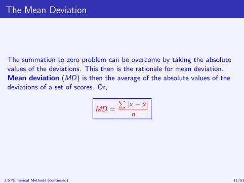
The summation to zero problem can be overcome by taking the absolutevalues of the deviations. This then is the rationale for mean deviation.Mean deviation (MD) is then the average of the absolute values of thedeviations of a set of scores. Or,
MD =
∑|x − x̄ |n
2.6 Numerical Methods (continued) 11/53
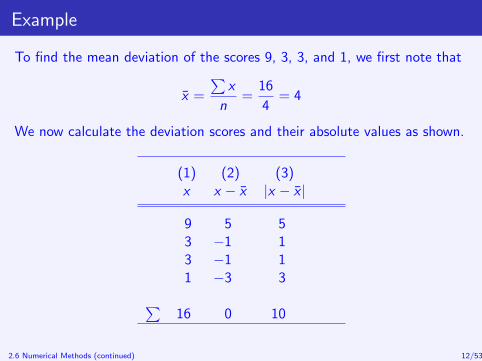
Example
To find the mean deviation of the scores 9, 3, 3, and 1, we first note that
x̄ =
∑x
n=
16
4= 4
We now calculate the deviation scores and their absolute values as shown.
(1) (2) (3)x x − x̄ |x − x̄ |
9 5 53 −1 13 −1 11 −3 3∑
16 0 10
2.6 Numerical Methods (continued) 12/53
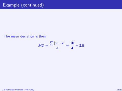
Example (continued)
The mean deviation is then
MD =
∑|x − x̄ |n
=10
4= 2.5
2.6 Numerical Methods (continued) 13/53
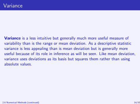
Variance
Variance is a less intuitive but generally much more useful measure ofvariability than is the range or mean deviation. As a descriptive statisticvariance is less appealing than is mean deviation but is generally moreuseful because of its role in inference as will be seen. Like mean deviation,variance uses deviations as its basis but squares them rather than usingabsolute values.
2.6 Numerical Methods (continued) 14/53
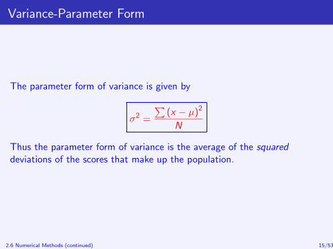
Variance-Parameter Form
The parameter form of variance is given by
σ2 =
∑(x − µ)2
N
Thus the parameter form of variance is the average of the squareddeviations of the scores that make up the population.
2.6 Numerical Methods (continued) 15/53
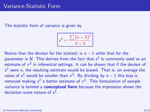
Variance-Statistic Form
The statistic form of variance is given by
s2 =
∑(x − x̄)2
n − 1
Notice that the devisor for the statistic is n − 1 while that for theparameter is N. This derives from the fact that s2 is commonly used as anestimate of σ2 in inferential settings. It can be shown that if the devisor ofs2 were n, the resulting estimate would be biased. That is, on average thevalue of s2 would be smaller than σ2. By dividing by n − 1 this bias isremoved making s2 a better estimate of σ2. This formulation of samplevariance is termed a conceptual form because the expression shows thedeviation score nature of s2.
2.6 Numerical Methods (continued) 16/53

Alternative Expression For s2
An algebraically equivalent expression for s2 that is useful forcomputations is given by
s2 =
∑x2 − (
Px)2
n
n − 1
2.6 Numerical Methods (continued) 17/53

Example
To calculate the variance of the values 9, 3, 3, and 1 via the conceptualmethod we arrange the data as follows.
(1) (2) (3)
x x − x̄ (x − x̄)2
9 5 253 −1 13 −1 11 −3 9∑
16 0 36
2.6 Numerical Methods (continued) 18/53

Example (continued)
We then calculate
s2 =
∑(x − x̄)2
n − 1
=36
3= 12
2.6 Numerical Methods (continued) 19/53
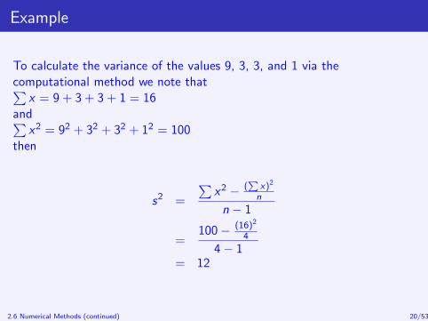
Example
To calculate the variance of the values 9, 3, 3, and 1 via thecomputational method we note that∑
x = 9 + 3 + 3 + 1 = 16and∑
x2 = 92 + 32 + 32 + 12 = 100then
s2 =
∑x2 − (
Px)2
n
n − 1
=100 − (16)2
4
4 − 1= 12
2.6 Numerical Methods (continued) 20/53
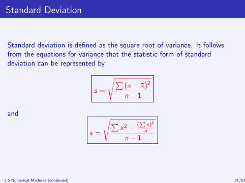
Standard Deviation
Standard deviation is defined as the square root of variance. It followsfrom the equations for variance that the statistic form of standarddeviation can be represented by
s =
√∑(x − x̄)2
n − 1
and
s =
√∑x2 − (
Px)2
n
n − 1
2.6 Numerical Methods (continued) 21/53
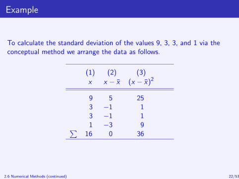
Example
To calculate the standard deviation of the values 9, 3, 3, and 1 via theconceptual method we arrange the data as follows.
(1) (2) (3)
x x − x̄ (x − x̄)2
9 5 253 −1 13 −1 11 −3 9∑
16 0 36
2.6 Numerical Methods (continued) 22/53

Example (continued)
We then calculate
s =
√∑(x − x̄)2
n − 1
=
√36
3= 3.464
2.6 Numerical Methods (continued) 23/53

Example
To calculate the standard deviation of the values 9, 3, 3, and 1 via thecomputational method we note that∑
x = 9 + 3 + 3 + 1 = 16and∑
x2 = 92 + 32 + 32 + 12 = 100then
s =
√∑x2 − (
Px)2
n
n − 1
=
√100 − (16)2
4
4 − 1= 3.464
2.6 Numerical Methods (continued) 24/53

Measures of Relative Position
Measures of relative position are methods that locate the relative positionsof observations in a distribution. To this end we will in turn examinepercentiles, percentile ranks, and z scores.
2.6 Numerical Methods (continued) 25/53

Percentiles
There is no standard definition for percentile. We will use the following. Apercentile is a point on the scale of measurement below which a specifiedpercentage of the observations are located. By this definition, the (scalebased) median can be defined as the fiftieth percentile.An expression for a given percentile is provided by
Pp = LRL + (w)
[(pr) (n) − cf
f
]where Pp represents the pth percentile, LRL is the lower real limit of theinterval that contains the pth percentile, w is the width of the intervalcalculated as the difference between the upper and lower real limits of thatinterval, pr is p expressed as a proportion (i.e., p/100), n is the totalnumber of observations, cf is the cumulative frequency up to thepercentile interval and f is the frequency of that interval.
2.6 Numerical Methods (continued) 26/53

Three Scenarios
When computing a percentile, three different scenarios are possible.
When a percentile interval is identified, the percentile formula isapplied.
When the sought proportion of observations falls below a real limitwith the interval above the limit having nonzero frequency, the reallimit is taken as the percentile.
When the sought proportion of observations falls below a real limitwith the interval above the limit having zero frequency, the midpointof the zero frequency interval(s) is taken as the sought percentile.
2.6 Numerical Methods (continued) 27/53
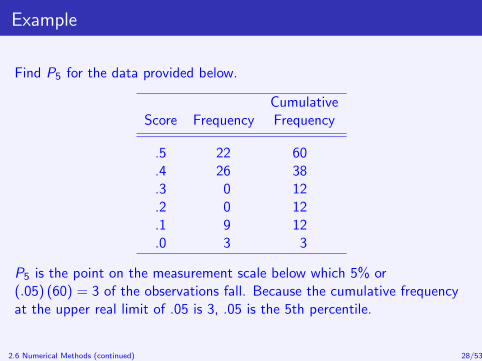
Example
Find P5 for the data provided below.
CumulativeScore Frequency Frequency
.5 22 60
.4 26 38
.3 0 12
.2 0 12
.1 9 12
.0 3 3
P5 is the point on the measurement scale below which 5% or(.05) (60) = 3 of the observations fall. Because the cumulative frequencyat the upper real limit of .05 is 3, .05 is the 5th percentile.
2.6 Numerical Methods (continued) 28/53

Example
Find P20 for the data provided below.
CumulativeScore Frequency Frequency
.5 22 60
.4 26 38
.3 0 12
.2 0 12
.1 9 12
.0 3 3
Since (.2) (60) = 12 of the observations fall below any point between .15and .35, the midpoint of .25 is taken as the 20th percentile.
2.6 Numerical Methods (continued) 29/53
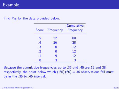
Example
Find P60 for the data provided below.
CumulativeScore Frequency Frequency
.5 22 60
.4 26 38
.3 0 12
.2 0 12
.1 9 12
.0 3 3
Because the cumulative frequencies up to .35 and .45 are 12 and 38respectively, the point below which (.60) (60) = 36 observations fall mustbe in the .35 to .45 interval.
2.6 Numerical Methods (continued) 30/53

Example (continued)
Applying Equation 2.5 gives
P60 = LRL + (w)
[(pr) (n) − cf
f
]= .35 + (.10)
[(.60) (60) − 12
26
]= .442
2.6 Numerical Methods (continued) 31/53
Percentile Rank
While a percentile is a point on the scale of measurement below which agiven percentage of observations fall, a percentile rank is the percentageof observations that fall below a given point on the scale. Thus,percentiles are points and percentile ranks are percentages. Because oftheir close relationship, they are often confused.
2.6 Numerical Methods (continued) 32/53

Percentile Rank (continued)
When the scale point whose percentile rank is sought falls in a nonzerofrequency interval, the following equation can be used to find percentileranks.
PRP =100
[f (P−LRL)
w + cf]
n
where P is the point on the scale for which the percentile rank is to becalculated, LRL is the lower real limit of the interval containing P, w isthe width of the interval calculated as the difference between the upperand lower real limits of that interval, n is the total number of observations,cf is the cumulative frequency up to the interval containing P and f is thefrequency of that interval.
2.6 Numerical Methods (continued) 33/53
Percentile Rank (continued)
When the point falls at the upper (lower) real limit of an interval or in aninterval with zero frequency, we use
PRP = 100cf
n
where cf is the cumulative frequency up to the point.
2.6 Numerical Methods (continued) 34/53
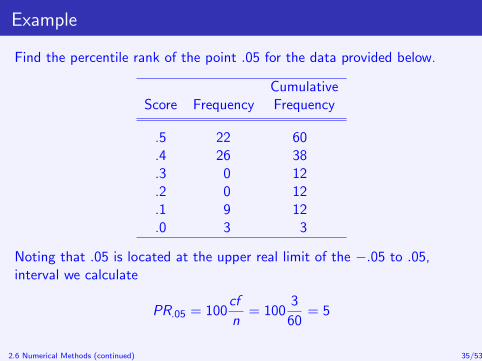
Example
Find the percentile rank of the point .05 for the data provided below.
CumulativeScore Frequency Frequency
.5 22 60
.4 26 38
.3 0 12
.2 0 12
.1 9 12
.0 3 3
Noting that .05 is located at the upper real limit of the −.05 to .05,interval we calculate
PR.05 = 100cf
n= 100
3
60= 5
2.6 Numerical Methods (continued) 35/53
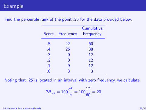
Example
Find the percentile rank of the point .25 for the data provided below.
CumulativeScore Frequency Frequency
.5 22 60
.4 26 38
.3 0 12
.2 0 12
.1 9 12
.0 3 3
Noting that .25 is located in an interval with zero frequency, we calculate
PR.25 = 100cf
n= 100
12
60= 20
2.6 Numerical Methods (continued) 36/53

Example
Find the percentile rank of the point .442 for the data provided below.
CumulativeScore Frequency Frequency
.5 22 60
.4 26 38
.3 0 12
.2 0 12
.1 9 12
.0 3 3
Noting that .442 is located in the interval .35 to .45, we calculate
PR.442 =100
[f (P−LRL)
w + cf]
n=
100[
26(.442−.35).1 + 12
]60
= 60
2.6 Numerical Methods (continued) 37/53
Percentile Ranks of Scores
Unfortunately, data analysts are usually not interested in finding thepercentile rank of a point on the measurement scale, but rather want toknow the percentile rank of a score or observation. This presents adifficulty since, scores are not points on the scale but rather, representintervals. How then do you find the percentile rank of a score?
2.6 Numerical Methods (continued) 38/53

Percentile Ranks of Scores
Basically, you must choose a point on the scale to represent the score.Three common choices are used.
1 The lower real limit of the score interval.
2 The midpoint of the score interval.
3 The upper real limit of the score interval.
2.6 Numerical Methods (continued) 39/53
z Scores
Percentiles locate points relative to all the observations in a data set. Bycontrast, z scores locate points relative to the mean of the data. Moreprecisely, a z score indicates the distance and direction of a point from themean in terms of standard units.
2.6 Numerical Methods (continued) 40/53
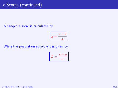
z Scores (continued)
A sample z score is calculated by
z =x − x̄
s
While the population equivalent is given by
Z =x − µ
σ
2.6 Numerical Methods (continued) 41/53

Example
Convert the set of scores 1, 3, 3, and 9 to z scores. Then find the meanand standard deviation of the z scores.The mean and standard deviation of the original data are, respectively, 4and 3.46. Using these values in Equation 2.2.3 gives
z1 = 1−43.46 = −.867
z3 = 3−43.46 = −.289
z3 = 3−43.46 = −.289
z9 = 9−43.46 = 1.445
2.6 Numerical Methods (continued) 42/53
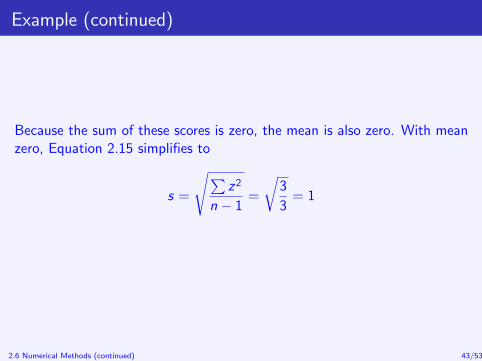
Example (continued)
Because the sum of these scores is zero, the mean is also zero. With meanzero, Equation 2.15 simplifies to
s =
√∑z2
n − 1=
√3
3= 1
2.6 Numerical Methods (continued) 43/53

Measures of Distribution Shape
Certain aspects of distribution shapes can be characterized numerically.The two most common of these, skew and kurtosis, will be discussed here
2.6 Numerical Methods (continued) 44/53

Skew
Various methods have been developed to numerically describe the amountof skew (or lack thereof) that characterizes a distribution. Skewisgenerally defined as the degree of asymmetry in a distribution.
2.6 Numerical Methods (continued) 45/53
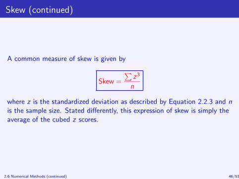
Skew (continued)
A common measure of skew is given by
Skew =
∑z3
n
where z is the standardized deviation as described by Equation 2.2.3 and nis the sample size. Stated differently, this expression of skew is simply theaverage of the cubed z scores.
2.6 Numerical Methods (continued) 46/53
Skew (continued)
When this expression results in a negative or positive value, thedistribution is said to be negatively or positively skewed respectively. Whenthe value is zero the distribution is said to be symmetric. The followingare depictions of each type.
2.6 Numerical Methods (continued) 47/53

Skew (continued)
0.0
1
2
3
4
5
0.0
1
2
3
4
5
0.0
1
2
3
4
5
Negatively
Skewed
Positively
Skewed
Symmetric
1 2 3 4 5 6 7
1 2 3 4 5 6 7
1 2 3 4 5 6 7
A
B
C
Fre
quen
cyF
requ
ency
Fre
qu
ency
2.6 Numerical Methods (continued) 48/53
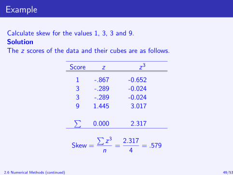
Example
Calculate skew for the values 1, 3, 3 and 9.SolutionThe z scores of the data and their cubes are as follows.
Score z z3
1 -.867 -0.6523 -.289 -0.0243 -.289 -0.0249 1.445 3.017∑
0.000 2.317
Skew =
∑z3
n=
2.317
4= .579
2.6 Numerical Methods (continued) 49/53

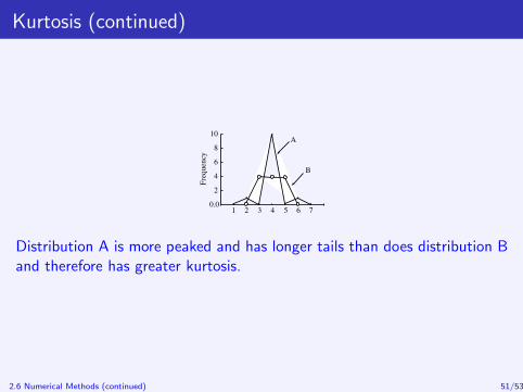
Kurtosis
Kurtosis refers to the peakedness of a distribution relative to the lengthand size of its tails. Distributions with sharp peaks are said to beleptokurtic while those that have flattened middles are said to beplatykurtic. Kurtosis pertains to distributions with no more than onemode.
2.6 Numerical Methods (continued) 50/53
Kurtosis (continued)
1 2 3 4 5 6 70.0
2
4
6
8
10A
B
Fre
qu
ency
Distribution A is more peaked and has longer tails than does distribution Band therefore has greater kurtosis.
2.6 Numerical Methods (continued) 51/53
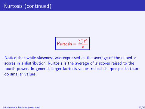
Kurtosis (continued)
Kurtosis =
∑z4
n
Notice that while skewness was expressed as the average of the cubed zscores in a distribution, kurtosis is the average of z scores raised to thefourth power. In general, larger kurtosis values reflect sharper peaks thando smaller values.
2.6 Numerical Methods (continued) 52/53

Example
Calculate kurtosis for the values 1, 3, 3 and 9.SolutionThe z scores of the data with their values raised to the fourth power are asfollows.
Score z z4
1 -.867 0.5653 -.289 0.0073 -.289 0.0079 1.445 4.360∑
0.000 4.939
Kurtosis =
∑z4
n=
4.939
4= 1.235
2.6 Numerical Methods (continued) 53/53


