
1
� A. J. Clark School of Engineering �Department of Civil and Environmental Engineering
by
Dr. Ibrahim A. AssakkafSpring 2001
ENCE 203 - Computation Methods in Civil Engineering IIDepartment of Civil and Environmental Engineering
University of Maryland, College Park
CHAPTER 7c. DIFFERENTIATION AND INTEGRATION
© Assakkaf
Slide No. 74
� A. J. Clark School of Engineering � Department of Civil and Environmental Engineering
ENCE 203 � CHAPTER 7c. DIFFERENTIATION AND INTEGRATION
Numerical Integration
� In calculus, integration is used to find the area under the curve.
� In engineering applications, the area under the curve can have physical interpretation and implications.
� For example, it can mean finding the total energy or rate of flow Q through a cross section of a river.

2
© Assakkaf
Slide No. 75
� A. J. Clark School of Engineering � Department of Civil and Environmental Engineering
ENCE 203 � CHAPTER 7c. DIFFERENTIATION AND INTEGRATION
Numerical Integration
� Area Under the Curvey = f(x)
xxa xb
( )∫=b
a
x
x
dxxf area
y = f(x)
xxa xb
( )∫=b
a
x
x
dxxf area
© Assakkaf
Slide No. 76
� A. J. Clark School of Engineering � Department of Civil and Environmental Engineering
ENCE 203 � CHAPTER 7c. DIFFERENTIATION AND INTEGRATION
Numerical Integration
� Examples
( )( ) ( )
cxex
dxxexdxxfydx
xexxfy
x
x
x
+−−=
+−==⇒
+−==
∫∫ ∫cos
4
sin
sin
4
3
3
( ) ( )21
21
1)(1
0
21
0
1
0
=
+=+==
+==
∫∫xxdxxdxxfI
xxfy

3
© Assakkaf
Slide No. 77
� A. J. Clark School of Engineering � Department of Civil and Environmental Engineering
ENCE 203 � CHAPTER 7c. DIFFERENTIATION AND INTEGRATION
Numerical Integration
� Need for Numerical IntegrationIn general, the function to be integrated will
typically be in one of the following forms:1. A simple continuous linear function such as a
polynomial, an exponential, or trigonometric function, such as
( )( )( ) xxf
exfxxxf
x
sin321
20232
5
+=−=
+−=
© Assakkaf
Slide No. 78
� A. J. Clark School of Engineering � Department of Civil and Environmental Engineering
ENCE 203 � CHAPTER 7c. DIFFERENTIATION AND INTEGRATION
Numerical Integration
� Need for Numerical Integration2. A complex non-linear continuous function that
is difficult or impossible to integrate directly such as
( )
( ) ( )
( )x
xxxx
exf
exxx
xxf
xxxxf
x
x
cosln3
tan1cos1
sin1
2
4
23
−++
=
−+−=
+++=
4
© Assakkaf
Slide No. 79
� A. J. Clark School of Engineering � Department of Civil and Environmental Engineering
ENCE 203 � CHAPTER 7c. DIFFERENTIATION AND INTEGRATION
Numerical Integration
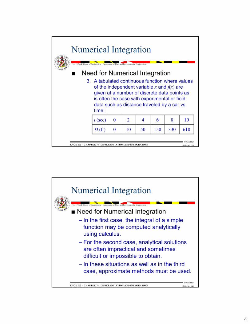
� Need for Numerical Integration3. A tabulated continuous function where values
of the independent variable x and f(x) are given at a number of discrete data points as is often the case with experimental or field data such as distance traveled by a car vs. time:
61033015050100D (ft)
1086420t (sec)
© Assakkaf
Slide No. 80
� A. J. Clark School of Engineering � Department of Civil and Environmental Engineering
ENCE 203 � CHAPTER 7c. DIFFERENTIATION AND INTEGRATION
Numerical Integration
� Need for Numerical Integration� In the first case, the integral of a simple
function may be computed analytically using calculus.
� For the second case, analytical solutions are often impractical and sometimes difficult or impossible to obtain.
� In these situations as well as in the third case, approximate methods must be used.

5
© Assakkaf
Slide No. 81
� A. J. Clark School of Engineering � Department of Civil and Environmental Engineering
ENCE 203 � CHAPTER 7c. DIFFERENTIATION AND INTEGRATION
Numerical Integration
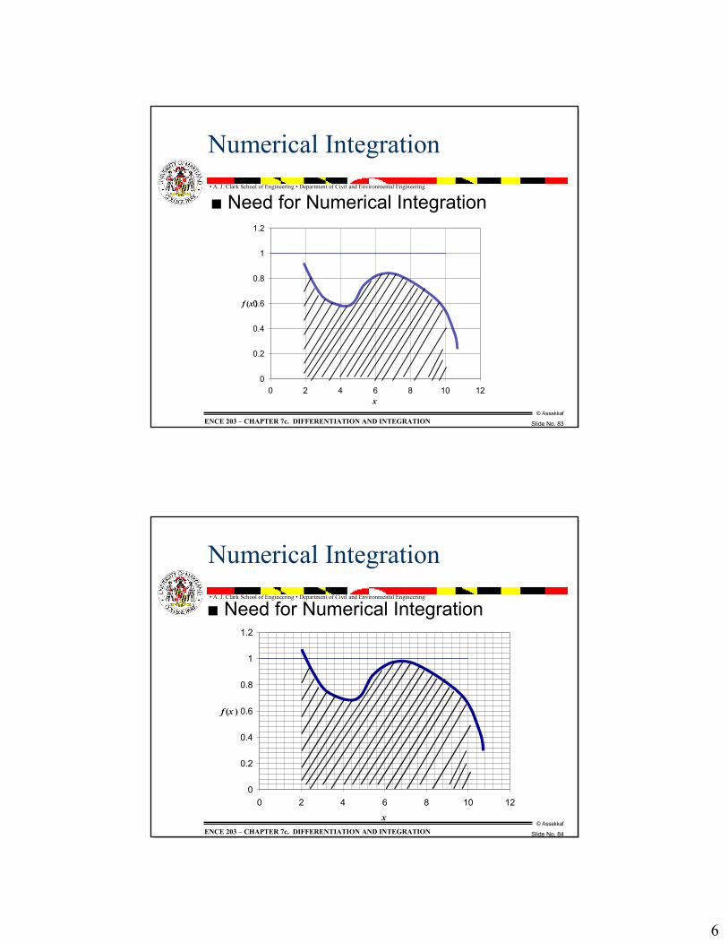
� Need for Numerical Integration� Pre computers and computational devices,
a visually oriented approach were used to integrate tabulated data and complicated functions.
� In this approach, the function is plotted on a grid (see figure), and the number of boxes that approximate the area are counted.
© Assakkaf
Slide No. 82
� A. J. Clark School of Engineering � Department of Civil and Environmental Engineering
ENCE 203 � CHAPTER 7c. DIFFERENTIATION AND INTEGRATION
Numerical Integration
� Need for Numerical Integration� This number is multiplied by the area of
each box to give a rough estimate of the total area under the curve.
� This estimate can be refined at the expense of additional effort by using a finer grid.
6
© Assakkaf
Slide No. 83
� A. J. Clark School of Engineering � Department of Civil and Environmental Engineering
ENCE 203 � CHAPTER 7c. DIFFERENTIATION AND INTEGRATION
Numerical Integration
� Need for Numerical Integration
0
0.2
0.4
0.6
0.8
1
1.2
0 2 4 6 8 10 12x
f (x )
© Assakkaf
Slide No. 84
� A. J. Clark School of Engineering � Department of Civil and Environmental Engineering
ENCE 203 � CHAPTER 7c. DIFFERENTIATION AND INTEGRATION
Numerical Integration
� Need for Numerical Integration
0
0.2
0.4
0.6
0.8
1
1.2
0 2 4 6 8 10 12x
f (x )

7
© Assakkaf
Slide No. 85
� A. J. Clark School of Engineering � Department of Civil and Environmental Engineering
ENCE 203 � CHAPTER 7c. DIFFERENTIATION AND INTEGRATION
Numerical Integration
� Engineering Applications� A surveyor might need to know the area of a
piece of land bounded by a meandering stream and two roads
© Assakkaf
Slide No. 86
� A. J. Clark School of Engineering � Department of Civil and Environmental Engineering
ENCE 203 � CHAPTER 7c. DIFFERENTIATION AND INTEGRATION
Numerical Integration
� Engineering Applications� A water-resource engineer might need to know
the cross-sectional area of a river to calculate the rate of flow Q.
VAVdAQ == ∫

8
© Assakkaf
Slide No. 87
� A. J. Clark School of Engineering � Department of Civil and Environmental Engineering
ENCE 203 � CHAPTER 7c. DIFFERENTIATION AND INTEGRATION
Numerical Integration
� Engineering Applications� A structural engineer might need to determine
the net lateral force due to non-uniform wind blowing against a side of a tall building.
© Assakkaf
Slide No. 88
� A. J. Clark School of Engineering � Department of Civil and Environmental Engineering
ENCE 203 � CHAPTER 7c. DIFFERENTIATION AND INTEGRATION
Numerical Integration
� Integration Using Interpolating Polynomial
� The general form of an interpolating polynomial is given by
� This polynomial can be integrated analytically as follows:
( ) nn xbxbxbxbbxf +++++= L3
32
210
( )132
11
32
21
0 ++++++=
+−∫ n
xbn
xbxbxbxbdxxfn
nn
nK

9
© Assakkaf
Slide No. 89
� A. J. Clark School of Engineering � Department of Civil and Environmental Engineering
ENCE 203 � CHAPTER 7c. DIFFERENTIATION AND INTEGRATION
Numerical Integration
� Integration Using Interpolating Polynomial� The Gregory-Newton method for deriving
an interpolation formula can also be used to evaluate the integral of a function.
� Recall G-N method:
( ) ( ) ( )( ) ( )( )( )( )( ) ( ) ( )( ) ( )nnnn xxxxxxaxxxxxxa
xxxxxxaxxxxaxxaaxf−−−+−−−+
−−−+−−+−+=
+− KK 211121
3214213121
© Assakkaf
Slide No. 90
� A. J. Clark School of Engineering � Department of Civil and Environmental Engineering
ENCE 203 � CHAPTER 7c. DIFFERENTIATION AND INTEGRATION
Numerical Integration
� Integration Using Interpolating Polynomial
� The terms could be rearrange to form an nth-order polynomial of the type
� This polynomial can be integrated analytically as
( ) 11
21 +− +++= n
nn bxbxbxf L
( ) xbxnbx
nbdxxf n
nn1
211
1 ++ +++
+=∫ L

10
© Assakkaf
Slide No. 91
� A. J. Clark School of Engineering � Department of Civil and Environmental Engineering
ENCE 203 � CHAPTER 7c. DIFFERENTIATION AND INTEGRATION
Numerical Integration
� Example 1Derive a second-degree interpolation polynomial to fit the following data points, and then using the fitted polynomial to approximate
Compare your result with that of the exact integral (i.e., x4/4).
2781f(x)321x
( )∫5.2
5.1
dxxf
© Assakkaf
Slide No. 92
� A. J. Clark School of Engineering � Department of Civil and Environmental Engineering
ENCE 203 � CHAPTER 7c. DIFFERENTIATION AND INTEGRATION
Numerical Integration
� Example 1 (cont�d)� The general form of the interpolation
polynomial is given by
� In our case it is
( ) nn xbxbxbxbbxf +++++= L3
32
210
( ) 2210 xbxbbxf ++=
11
© Assakkaf
Slide No. 93
� A. J. Clark School of Engineering � Department of Civil and Environmental Engineering
ENCE 203 � CHAPTER 7c. DIFFERENTIATION AND INTEGRATION
Numerical Integration
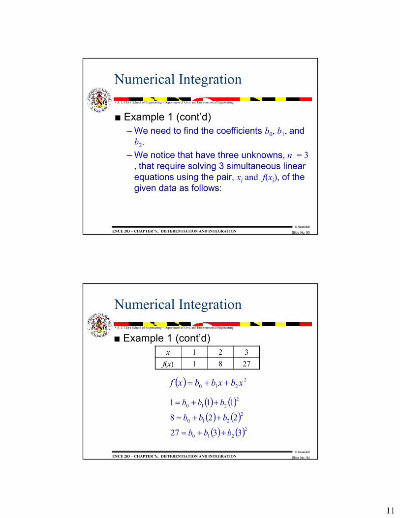
� Example 1 (cont�d)� We need to find the coefficients b0, b1, and
b2.� We notice that have three unknowns, n = 3
, that require solving 3 simultaneous linear equations using the pair, xi and f(xi), of the given data as follows:
© Assakkaf
Slide No. 94
� A. J. Clark School of Engineering � Department of Civil and Environmental Engineering
ENCE 203 � CHAPTER 7c. DIFFERENTIATION AND INTEGRATION
Numerical Integration
� Example 1 (cont�d)
( ) ( )( ) ( )
( ) ( )2210
2210
2210
3327
228
111
bbb
bbb
bbb
++=
++=
++=
( ) 2210 xbxbbxf ++=
2781f(x)321x

12
© Assakkaf
Slide No. 95
� A. J. Clark School of Engineering � Department of Civil and Environmental Engineering
ENCE 203 � CHAPTER 7c. DIFFERENTIATION AND INTEGRATION
Numerical Integration
� Example 1 (cont�d)
� OR
=
2781
931421111
2
1
0
bbb
27938421
210
210
210
=++=++=++
bbbbbbbbb
© Assakkaf
Slide No. 96
� A. J. Clark School of Engineering � Department of Civil and Environmental Engineering
ENCE 203 � CHAPTER 7c. DIFFERENTIATION AND INTEGRATION
Numerical Integration
� Example 1 (cont�d)� The solution of this set of equations yields
� Therefore, the interpolation polynomial is
� And its anti-derivative (integral) is
−=
6116
2
1
0
bbb
( ) 2210 xbxbbxf ++=
( ) 26116 xxxf +−=
( ) cxxxdxxf ++−=∫ 32
36
2116

13
© Assakkaf
Slide No. 97
� A. J. Clark School of Engineering � Department of Civil and Environmental Engineering
ENCE 203 � CHAPTER 7c. DIFFERENTIATION AND INTEGRATION
Numerical Integration
� Example 1 (cont�d)The result is
( )
( ) ( ) ( ) ( ) ( ) ( )
5.8 375.3875.11
5.125.12
115.165.225.22
115.26
22
116
3232
5.2
5.1
325.2
5.1
=−=
+−−
+−=
+−=∫ xxxdxxf
© Assakkaf
Slide No. 98
� A. J. Clark School of Engineering � Department of Civil and Environmental Engineering
ENCE 203 � CHAPTER 7c. DIFFERENTIATION AND INTEGRATION
Numerical Integration
� Example 1 (cont�d)� Evaluation of the exact integral is as
follows:
� In this example, the approximation is identical to the true value.
( ) ( ) ( ) 5.84
5.15.24
445.2
5.1
45.2
5.1
35.2
5.1
=−=== ∫∫xxdxxf
14
© Assakkaf
Slide No. 99
� A. J. Clark School of Engineering � Department of Civil and Environmental Engineering
ENCE 203 � CHAPTER 7c. DIFFERENTIATION AND INTEGRATION
Numerical Integration
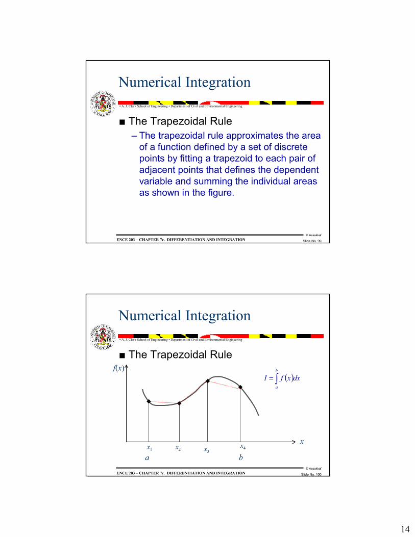
� The Trapezoidal Rule� The trapezoidal rule approximates the area
of a function defined by a set of discrete points by fitting a trapezoid to each pair of adjacent points that defines the dependent variable and summing the individual areas as shown in the figure.
© Assakkaf
Slide No. 100
� A. J. Clark School of Engineering � Department of Civil and Environmental Engineering
ENCE 203 � CHAPTER 7c. DIFFERENTIATION AND INTEGRATION
Numerical Integration
� The Trapezoidal Rule
a b
x
f(x)
x4x3x2x1
( )∫=b
a
dxxfI

15
© Assakkaf
Slide No. 101
� A. J. Clark School of Engineering � Department of Civil and Environmental Engineering
ENCE 203 � CHAPTER 7c. DIFFERENTIATION AND INTEGRATION
Numerical Integration
� The Trapezoidal Rule� Derivation
� The trapezoidal rule can be derived by fitting a linear interpolating polynomial to each pair of points.
� Using, for example Gregory-Newton formula, an expression for a linear polynomial can be obtained as follows:
( ) ( ) ( )( ) ( )( )( )( )( ) ( ) ( )( ) ( )nnnn xxxxxxaxxxxxxa
xxxxxxaxxxxaxxaaxf−−−+−−−+
−−−+−−+−+=
+− KK 211121
3214213121
© Assakkaf
Slide No. 102
� A. J. Clark School of Engineering � Department of Civil and Environmental Engineering
ENCE 203 � CHAPTER 7c. DIFFERENTIATION AND INTEGRATION
Numerical Integration
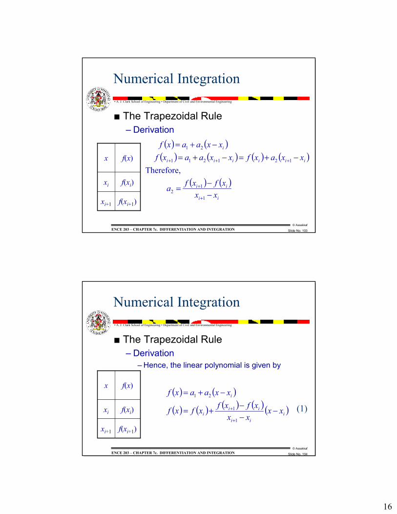
� The Trapezoidal Rule� Derivation
� If we denote the values of the two independent variables as xi and xi+1, then G-N formula gives
( ) ( )( ) ( )( ) 1
21
21
axfxxaaxf
xxaaxf
i
iii
i
=−+=
−+=
f(xi+1)xi+1
f(xi)xi
f(x)x
16
© Assakkaf
Slide No. 103
� A. J. Clark School of Engineering � Department of Civil and Environmental Engineering
ENCE 203 � CHAPTER 7c. DIFFERENTIATION AND INTEGRATION
Numerical Integration
� The Trapezoidal Rule� Derivation
( ) ( )( ) ( ) ( ) ( )
( ) ( )ii
ii
iiiiii
i
xxxfxfa
xxaxfxxaaxfxxaaxf
−−=
−+=−+=−+=
+
+
+++
1
12
121211
21
Therefore,
f(xi+1)xi+1
f(xi)xi
f(x)x
© Assakkaf
Slide No. 104
� A. J. Clark School of Engineering � Department of Civil and Environmental Engineering
ENCE 203 � CHAPTER 7c. DIFFERENTIATION AND INTEGRATION
Numerical Integration
� The Trapezoidal Rule� Derivation
� Hence, the linear polynomial is given by
( ) ( )
( ) ( ) ( ) ( )( )iii
iii
i
xxxx
xfxfxfxf
xxaaxf
−−−+=
−+=
+
+
1
1
21
f(xi+1)xi+1
f(xi)xi
f(x)x
(1)

17
© Assakkaf
Slide No. 105
� A. J. Clark School of Engineering � Department of Civil and Environmental Engineering
ENCE 203 � CHAPTER 7c. DIFFERENTIATION AND INTEGRATION
Numerical Integration
� The Trapezoidal Rule� Derivation
� Integrating Eq. 1 between two points, say a and b:
( ) ( ) ( ) ( ) ( )
( ) ( ) ( ) ( )
( ) ( ) ( ) ( )2
2
2
2
1
1
2
1
1
2
1
1
i
ii
iii
i
ii
iii
b
a
i
ii
iii
b
a
xaxx
xfxfaxf
xbxx
xfxfbxf
xxxx
xfxfxxfdxxf
−−−−−
−−−+=
−−−+=
+
+
+
+
+
+∫
© Assakkaf
Slide No. 106
� A. J. Clark School of Engineering � Department of Civil and Environmental Engineering
ENCE 203 � CHAPTER 7c. DIFFERENTIATION AND INTEGRATION
Numerical Integration
� The Trapezoidal Rule� Derivation
Or
Letting b = xi+1 and a = xi, results in
( ) ( ) ( ) ( )( ) ( ) ( )
−−−+
−−= +++
+∫ 111
1 2 iiiiiiii
b
a
xfxxfxxfxfabxx
abdxxf
( ) ( ) ( )[ ]iiii
x
x
xfxfxxdxxfi
i
+−= ++∫
+
11
2
1

18
© Assakkaf
Slide No. 107
� A. J. Clark School of Engineering � Department of Civil and Environmental Engineering
ENCE 203 � CHAPTER 7c. DIFFERENTIATION AND INTEGRATION
Numerical Integration
� The Trapezoidal RuleThe trapezoidal rule can be used to approximate the integral between two points x1 and xn of a function. It is given by
( ) ( ) ( ) ( )∑∫−
=
++
+−≈1
1
11 2
1
n
i
iiii
x
x
xfxfxxdxxfn
(2)
© Assakkaf
Slide No. 108
� A. J. Clark School of Engineering � Department of Civil and Environmental Engineering
ENCE 203 � CHAPTER 7c. DIFFERENTIATION AND INTEGRATION
Numerical Integration
� Geometric Interpretation the Trapezoidal Rule� The trapezoidal rule can also be derived
geometrically.� The trapezoidal rule is equivalent to
approximating the area of the trapezoid under the straight line connecting f(xi) andf(xi+1) as shown in the following figure:

19
© Assakkaf
Slide No. 109
� A. J. Clark School of Engineering � Department of Civil and Environmental Engineering
ENCE 203 � CHAPTER 7c. DIFFERENTIATION AND INTEGRATION
Numerical Integration
� Geometric Interpretation the Trapezoidal Rule
x
f(x)f(xi+1)
f(xi)
xi xi+1
© Assakkaf
Slide No. 110
� A. J. Clark School of Engineering � Department of Civil and Environmental Engineering
ENCE 203 � CHAPTER 7c. DIFFERENTIATION AND INTEGRATION
Numerical Integration
� Geometric Interpretation the Trapezoidal Rule� Recall from geometry that the formula for
computing the area of a trapezoid is the height times the average of the bases as shown in the figure.
� Therefore, the integral estimate can be represented as
height average width ×≈I

20
© Assakkaf
Slide No. 111
� A. J. Clark School of Engineering � Department of Civil and Environmental Engineering
ENCE 203 � CHAPTER 7c. DIFFERENTIATION AND INTEGRATION
Numerical Integration
� Geometric Interpretation the Trapezoidal Rule
Height
Base
Base
HeightHeight
Width
( ) ( ) ( )[ ]iiii
x
x
xfxfxxdxxfi
i
+−= ++∫
+
11
2
1
height average width ×≈I
© Assakkaf
Slide No. 112
� A. J. Clark School of Engineering � Department of Civil and Environmental Engineering
ENCE 203 � CHAPTER 7c. DIFFERENTIATION AND INTEGRATION
Numerical Integration
� Example 2Using the trapezoidal rule , estimate the area under the curve, that is
for the following function given in tabulated form:
3-3-13f(xi)4321xi
4321i
( )∫=4
1
dxxfI

21
© Assakkaf
Slide No. 113
� A. J. Clark School of Engineering � Department of Civil and Environmental Engineering
ENCE 203 � CHAPTER 7c. DIFFERENTIATION AND INTEGRATION
Numerical Integration
� Example 2 (cont�d)Using Eq. 2,
( ) ( ) ( ) ( )∑∫−
=
++
+−≈1
1
11 2
1
n
i
iiii
x
x
xfxfxxdxxfn
( ) ( )[ ] ( )[ ] ( )[ ]
1 0(-2)1
2)3(334
2)3(123
2)1(312
4
1
−=++=
−+−+−+−−+−+−≈∫ dxxf
3-3-13f(xi)4321xi
4321i
3-3-13f(xi)4321xi
4321i


